the Creative Commons Attribution 4.0 License.
the Creative Commons Attribution 4.0 License.
 | 17 Jun 2022
Development and parameter estimation of snowmelt models using spatial snow-cover observations from MODIS
Dhiraj Raj Gyawali
András Bárdossy
Given the importance of snow on different land and atmospheric processes, accurate representation of seasonal snow evolution, including distribution and melt volume, is highly imperative to any water resources development trajectories. The limitation of reliable snowmelt estimation in mountainous regions is, however, further exacerbated by data scarcity. This study attempts to develop relatively simple extended degree-day snow models driven by freely available snow-cover images. This approach offers relative simplicity and a plausible alternative to data-intensive models, as well as in situ measurements, and has a wide range of applicability, allowing for immediate verification with point measurements. The methodology employs readily available MODIS composite images to calibrate the snowmelt models on spatial snow distribution in contrast to the traditional snow-water-equivalent-based calibration. The spatial distribution of snow-cover is simulated using different extended degree-day models with parameters calibrated against individual MODIS snow-cover images for cloud-free days or a set of images representing a period within the snow season. The study was carried out in Baden-Württemberg (Germany) and in Switzerland. The simulated snow-cover data show very good agreement with MODIS snow-cover distribution, and the calibrated parameters exhibit relative stability across the time domain. Furthermore, different thresholds that demarcate snow and no-snow pixels for both observed and simulated snow cover were analyzed to evaluate these thresholds' influence on the model performance and identified for the study regions. The melt data from these calibrated snow models were used as standalone inputs to a modified Hydrologiska Byråns Vattenbalansavdelning (HBV) without the snow component in all the study catchments to assess the performance of the melt outputs in comparison to a calibrated standard HBV model. The results show an overall increase in Nash–Sutcliffe efficiency (NSE) performance and a reduction in uncertainty in terms of model performance. This can be attributed to the reduction in the number of parameters available for calibration in the modified HBV and an added reliability of the snow accumulation and melt processes inherent in the MODIS calibrated snow model output. This paper highlights that the calibration using readily available images used in this method allows for a flexible regional calibration of snow-cover distribution in mountainous areas with reasonably accurate precipitation and temperature data and globally available inputs. Likewise, the study concludes that simpler specific alterations to processes contributing to snowmelt can contribute to reliably identify the snow distribution and bring about improvements in hydrological simulations, owing to better representation of the snow processes in snow-dominated regimes.
- Article
(10571 KB) - Full-text XML
- BibTeX
- EndNote


Reliable representations of spatial distribution of seasonal snow and subsequent snowmelt are critical challenges for hydrological estimations, given their crucial relevance in mountainous regimes, especially because of the high sensitivity to climate change. Considering the snow effect on land and atmospheric processes, accurate representation of seasonal snow evolution is thus highly imperative to strengthen water resources development trajectories in these regions (Kirkham et al., 2019; Schmucki et al., 2014; He et al., 2014). Various modeling and measurement techniques are currently in practice which attempt to estimate the distribution of snow, but these methods have their own limitations. Prior studies on the comparison of snow models (Feng et al., 2008; Rutter et al., 2009) have highlighted the higher reliability of physically based approaches such as the energy balance approach in simulating the snow conditions. These complex models, although they offer a more realistic physical detail of the sub-processes (Wagner et al., 2009), are often associated with intensive data requirement, which is generally a big limitation in mountainous catchments around the world (Girons Lopez et al., 2020). Likewise, in situ measurements of snow depth providing accurate measures, seldom cover a wider spatial extent and are prone to be non-representative due to local influences. Lack of snow-depth information and, to some extent, persistent cloud cover in the mountains limit the standalone usage of remote sensing images in snow estimation (Tran et al., 2019). However, these images can provide a plausible alternative to ground-based data, especially in data-scarce mountainous regions, since their resolution and availability do not depend on the terrain (Parajka and Blöschl, 2008). The Moderate Resolution Imaging Spectroradiometer (MODIS) (Hall et al., 2006) aboard Terra and Aqua satellites provides one of the most extensively used snow-cover products worldwide, owing to its daily temporal resolution and a high spatial resolution of 500 m at the Equator. The MODIS snow-cover data performance, though seasonally and region dependent, has been found to be accurate enough for hydrological contexts (Parajka and Blöschl, 2008). The cloud obstruction in MODIS, though significant, can be reduced by combining the Aqua and Terra MODIS images and other spatiotemporal filtering techniques (Tran et al., 2019; Gafurov and Bárdossy, 2009; Wang and Xie, 2009).
Remote sensing integration in hydrological modeling has made important strides in recent years (Wagner et al., 2009). More so, several studies have been carried out by coupling satellite-based snow-cover information with hydrological models such as the ASCAT soil water index; MODIS snow-cover- and discharge-based calibration of a hydrological model (Tong et al., 2021); MODIS snow-cover-constrained multi-variable discharge calibration for hydrological models (Parajka and Blöschl, 2008; Udnæs et al., 2007); MODIS snow-covered-area-based calibration of a distributed hydrological model (Franz and Karsten, 2013); and model initialization (Liu et al., 2012). These studies highlight the value of MODIS snow-cover information in multi-variable calibration in addition to discharge, leading to a better representation of the hydrological processes, reduced uncertainty, and to some extent improved hydrological predictions. Apart from the multi-calibration approaches, Széles et al. (2020) implemented a step-based calibration technique to calibrate the individual modules of a hydrological model including snow, soil moisture, and runoff generation processes, which was concluded to be a well-informed runoff simulation. They used MODIS snow-cover data as a gap-filling information for the missing observed time-lapse photos of snow cover. Tekeli et al. (2005) used MODIS products in identifying the snow duration curve to be used in a snowmelt model and concluded that the coupling provides crucial information on snowmelt timing and magnitude. Likewise, there have been several studies to compare and improve the snow routine in various hydrological models in recent years. Girons Lopez et al. (2020) evaluated various formulations of the temperature index approach to analyze their response via the Hydrologiska Byråns Vattenbalansavdelning (HBV) model in 54 mountainous European catchments. Caicedo et al. (2012) also identified the best-performing variants of degree-day calculations for different regions in Colombia. They concluded that these specific targeted alterations improve the performance in terms of snow processes.
This paper draws its motivation from these studies to improve the simulation of snow accumulation and melt processes in data-scarce mountainous regions, using freely available data like MODIS snow-cover products. The widely used point-based snow depth and snow water equivalent measurements are often not representative due to the high variability of snow accumulation rendering calibration of snowmelt models based on point measurements highly uncertain. A standalone calibration of snowmelt modules based solely on pixel-wise MODIS snow-cover information was not found to be widely implemented. Franz and Karsten (2013) tested a MODIS fractional snow-cover area (SCA)-based calibration of a distributed hydrological model, SNOW17, with an areal snow depletion concept in which they concluded that calibrating only on MODIS SCA did not bring any improvement in the hydrological predictions. However, we identified the need to further explore the gap in exploiting the spatial distribution information of snow, which MODIS snow-cover data can provide on a daily basis and with a reasonable spatial detail. The purpose of this paper is, thus, to present a simple calibration method for snow accumulation and melt based on the satellite-based spatial binary (“snow”, “no-snow”) snow-cover information. This offers a wide range of applicability, allows for immediate verification with point measurements, and holds a high relevance in data-scarce regions, particularly in identifying time-continuous snow extents (with depth information) free from highly localized influences. The novelty of this study is to propose a standalone approach using MODIS snow-cover images for calibration of independent conceptual snowmelt models, thereby estimating model parameters from individual or sets of MODIS images. The data and the methodological approach can calibrate relatively complex snowmelt modules with reasonably accurate precipitation and temperature data without over-calibration, mainly owing to the robust binary data selected for calibration and the spatial extent of the satellite images. This also allows for the formulation of a flexible snowmelt module useful for distributed hydrologic modeling.
With the degree-day approach as a basis, we implemented different modifications to the snowmelt models incorporating different aspects governing snow hydrology such as precipitation-induced melt, radiation, and topography. For a better representation of the model performances, we evaluated the models in different layers of added detail. Sensitivity analyses for different thresholds that demarcate snow and no-snow pixels for both observed and simulated snow-cover in the study domain were carried out to evaluate these thresholds' influence on the model performances. To better understand and to validate the efficacy of the approach in terms of discharge, the calibrated melt outputs from the snowmelt model were also evaluated in a discharge-calibrated hydrological model. This allowed for the identification of more robust parameter sets, as the model uncertainty related to snow processes is significantly reduced. A simpler calibration of the hydrological models was achieved, as there were less parameters to be estimated. This approach also tends to reduce the hydrological model uncertainty as the set of equifinal parameters becomes smaller, which is a known challenge in hydrological modeling (Beven, 2001).
To develop and test simple snow models in mountainous or snow-dominated regions, the study area was selected as two distinct snow regimes: (a) characterized by intermittent snow and (b) characterized by partly longer-duration snow. For the former, Baden-Württemberg (BW) region in Germany was selected. Whole of Switzerland was considered to represent the longer-duration snow for the study. Figure 1 shows the study domain.
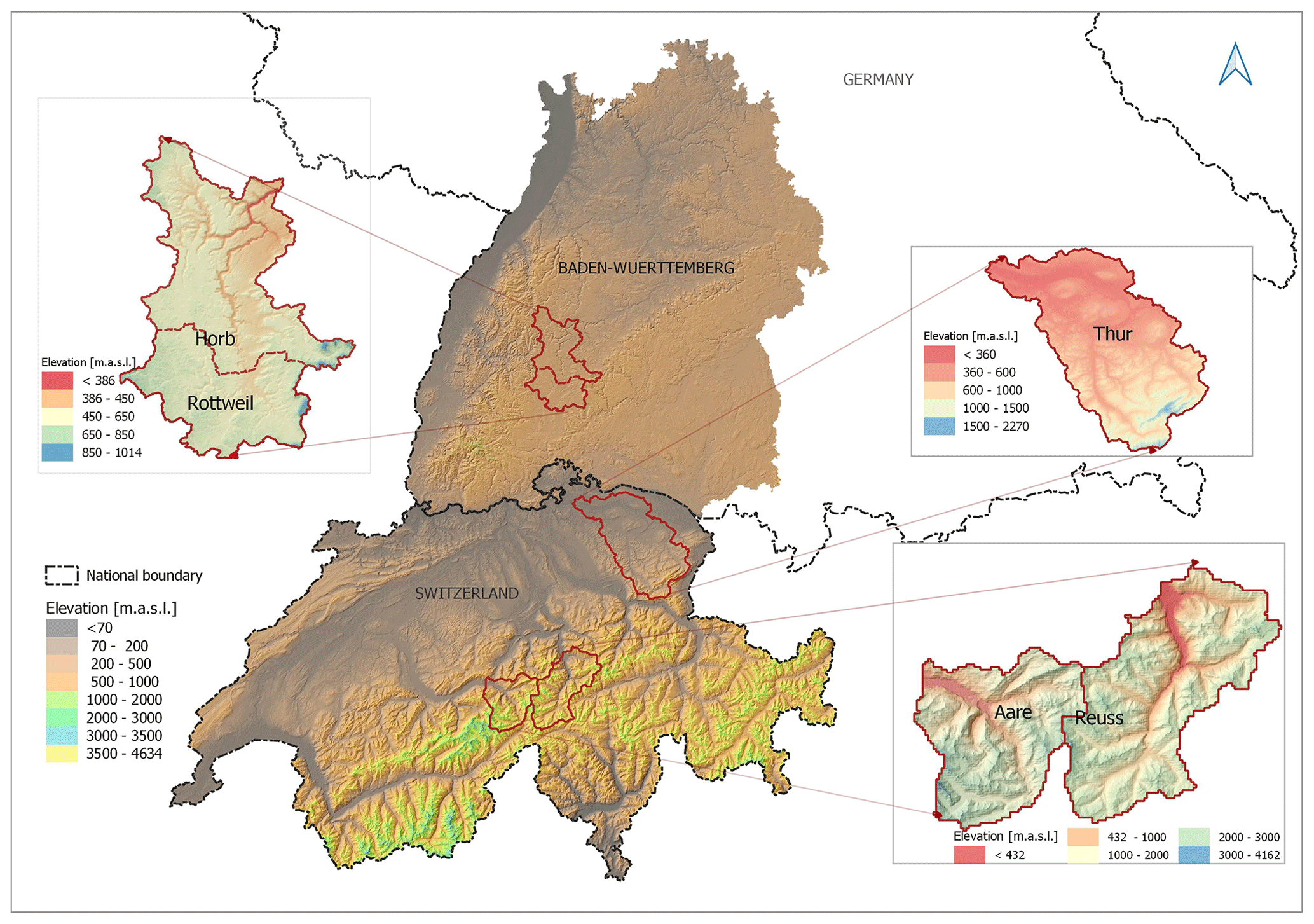
Figure 1Map of the study area with elevation.
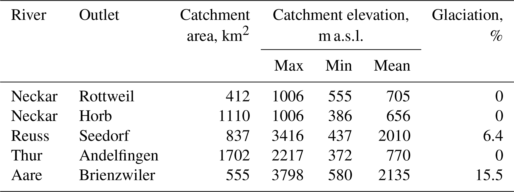
The BW region includes the Swabian Alps with an elevation rising to 1465 m a.s.l. from the lowest of 88 m a.s.l. Likewise, Switzerland includes the Swiss Alps region which covers the perennial snow/glacier area. The elevation ranges from below 200 to 4634 m a.s.l. The study areas exhibit an average snow season from October to April in Germany and September to June in Switzerland. For hydrological modeling, five catchments were selected (viz., Neckar catchments at Rottweil and Horb in BW and Reuss catchment at Seedorf, Aare catchment at Brienzwiler, and Thur catchment at Andelfingen in Switzerland). The Reuss and Aare catchments have a longer snow cover around the year and include glaciated areas. The properties of the catchments are shown in Table 1.
The data used for the study are the following:
-
Hydro-meteorology. Daily station meteorological data (viz. precipitation and minimum, maximum, and mean temperatures) from 2010–2018 were acquired for the study. For Germany, these variables were obtained from the Deutsche Wetterdienst (DWD), and for Switzerland they were obtained from the Federal Office of Meteorology and Climatology (MeteoSwiss). Likewise, daily discharge time series for selected catchments were acquired from the Bundesanstalt für Gewässerkunde (BFG) for Germany and the Federal Office for the Environment (FOEN) for Switzerland.
-
Topography. The Shuttle Radiation Topography Mission (SRTM) 90 m resolution digital elevation model (DEM) (Jarvis et al., 2008) was used in this study. The DEM was rescaled to match the MODIS resolution for consistency. Likewise, aspect and slope rasters were also obtained from this DEM.
-
Snow cover. Daily MODIS Terra and Aqua snow-cover data (version 6; Hall and Riggs, 2016) from 2010 to 2018 were used for calibrating the models and further analysis of snow distribution in the study regions. The resolution of the data is 500 m at the Equator.
This study presents a distributed modeling approach with model computations done at pixel level of a gridded domain of 464 m × 464 m grids. For this, the input data were preprocessed and interpolated onto the aforementioned grid cells. A gridded schema was extracted for both regions using the MODIS snow-cover data as a reference. This schema was considered the reference gridded domain for the data interpolation and model run.
2.1 MODIS preprocessing and cloud removal
The Aqua and Terra variants of MODIS snow-cover data were downloaded and then preprocessed. The preprocessed images were sequentially and spatiotemporally filtered using a cloud-removal procedure as described in Gafurov and Bárdossy (2009). The procedure follows the steps below:
-
The first step checks the Aqua–Terra image combination. Pixels with clouds (255) in one of the images and land (0) or snow (1–100) in the other were replaced with the snow/land value and vice versa. The output is a combined raster with reduced cloud pixels. The combined raster was then reclassified as “0” and “1”. No-snow pixel values of the combined raster (0) are set to “0”, and snow pixel values (1–100) are set to “1”. Everything else is set to “No data”.
-
The second step compares the preceding and succeeding days for a pixel under consideration. If both days for the pixels are cloud free with 0 or 1, the pixel under consideration will, respectively, get either 0 or 1 for the day.
-
Likewise, the third step compares the 2 d backward and 1 d forward and the 1 d backward and 2 d forward combination to check for cloud-free days and infill accordingly, assuming consecutive snow or no-snow days.
-
The fourth step compares the lowest elevation with snow and the highest elevation without snow for each day. Any pixel with elevation higher than the lowest elevation snow pixel would get “1”, and the elevation lower than the highest elevation without snow would get “0”.
-
The fifth step searches for “0” or “1” in an 8-pixel neighborhood surrounding the cell. If the neighborhood has a mode of at least four valid values, the pixel will then be either “0” or “1”.
2.2 Spatial interpolation of precipitation and temperature
Both BW and Switzerland have a well-distributed and dense network of meteorological stations. The daily precipitation and temperature values from these stations were used for geostatistical interpolation onto the aforementioned schema for the regions.
For the interpolation of temperature data, external drift kriging (EKD) was opted for in the regions under study, with station elevation as a drift (Hudson and Wackernagel, 1994). The station elevation exhibits strong correlation with the monthly and seasonal temperatures. Daily minimum, maximum, and mean temperatures from 85 stations in Baden-Württemberg and 365 stations for Switzerland were used for the interpolation. Cross-validation using leave-one-out approach was carried out to check for the applicability and the quality of the EKD interpolation.
For precipitation, the daily precipitation sums were interpolated onto the schema using a detrended residual kriging (RK) (Phillips et al., 1992; Martínez-Cob, 1996). To improve the precipitation interpolation in the higher elevation, a multiple linear regression (MLR) approach using directionally smoothed elevation was carried out for the study. Directional smoothing of elevation was done using half-space smoothing (Bárdossy and Pegram, 2013). The approach uses a directionally transformed and smoothed topography to identify the effect of directional advection for each day. Eight different directions, with 45∘ incremental angles, and three different smoothing distances (2, 3, and 5 km) were considered in this study. For each time step, a simple optimization was done to assess the correlation of the precipitation with the shifted DEMs, and the best direction and the smoothing radius for the time step were identified. This shifted and smoothed elevation was then used along with X and Y coordinates of the stations in the MLR to obtain precipitation estimates for stations. The residuals were then calculated for each day and ordinary kriging was carried out to obtain the kriged residuals. MLR-estimated precipitation surfaces for each time step using X and Y coordinates and shifted elevation for the grid points were then added to the Kriged residual surfaces to obtain the final precipitation estimates. In this study, 224 stations in BW and 449 stations in Switzerland were used. Leave-one-out cross-validation for each station was done for both variables.
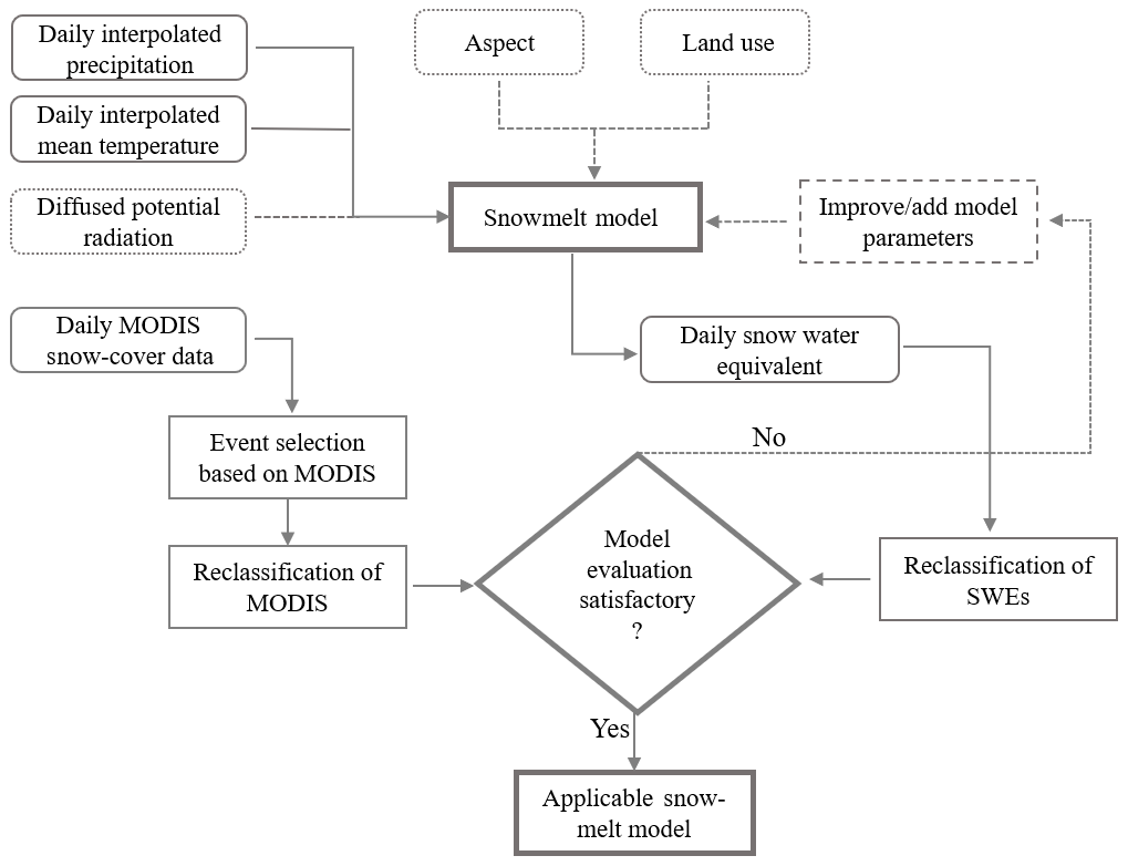
The methodological framework applied for the study is shown in Fig. 2 and is further discussed in subsequent sections.
3.1 Model variants
This study employs an empirical, temperature-index melt modeling approach using the degree-day factors. The degree-day models are widely used, owing to the relatively easier interpolation of air temperature and reasonable computational simplicity (Hock, 2003). This degree-day approach assumes melt rate as a linear function of the air temperature. Due to inherent large-scale spatial variability in mountainous regions, distributed meteorological inputs were employed to drive the different variants of the extended degree-day snowmelt models on a daily timescale. The major parameters used in the models are defined below:
-
precipitation amount at location x at time t (mm),
-
snow water equivalent amount at location x at time t (mm),
-
mean temperature at location x at time t (∘C),
-
water equivalent of precipitation falling as snow at location x at time t (mm),
-
melt water amount at location x at time t (mm),
-
TT= threshold critical temperature defining snow or no snow (∘C),
-
Ds= dry degree-day factor (mm ∘C−1),
-
maximum temperature at location x at time t (∘C),
-
minimum temperature at location x at time t (∘C),
-
scf = snow correction factor to account for the gauge undercatch of snow.
The following model variants were used to estimate the snow water equivalent (SWE, mm) and the resulting snow-cover in each pixel. Different nomenclatures are given in the models for the ease of understanding. Each successive model represents a gradual parameter-wise modification to the basic degree-day model.
3.1.1 Basic degree-day model (Model 1)
Model 1 is the most basic of all model variants. This model estimates the melt for each time step as a linear function of the difference between daily mean temperatures and a threshold temperature value, demarcating liquid precipitation and snow precipitation. A degree-day factor controls the rate of melt. Equation (1) calculates the amount of SWE available in pixel x at time t. Similarly, the snow precipitation and the resulting melt are calculated with Eqs. (2a) and (2b) as the model basis for each pixel; x in the study domain. A correction factor to account for the snowfall undercatch by the gauges and the vegetation interception “scf” is also used in this model and extended to all models in the study.
where
3.1.2 Wet degree-day model (Model 2)
To account for the melt induced by rain at temperatures higher than the critical threshold temperature, this variant adds a precipitation melt factor which controls the rate of melt based on air temperature and the precipitation amount falling on the pack. A similar approach was discussed in Bárdossy et al. (2020). This melt factor, henceforth referred to as Dw, increases the melt from Eq. (2b) on days with precipitation higher than a threshold value. For a given wet day, i.e., , the melt is calculated as in Eq. (3). For a dry day, melt is calculated as in Eq. (2b).
where
-
),
-
PT= threshold precipitation depth beyond which the liquid precipitation contributes to melt (mm),
-
Dw= the wet melt factor ((mm ∘C−1) mm−1),
-
combined melt factor on wet days (mm ∘C−1).
3.1.3 Wet degree-day model with snowfall and snowmelt temperatures (Model 3)
The instantaneous forms of precipitation as snow and liquid gives a clear indication of two temperature thresholds which demarcate the solid and liquid states of precipitation (Schaefli et al., 2005). This model includes different snowfall and snowmelt temperatures in Model 2 for a more accurate representation of the liquid-to-snow phase partition and melt initiation. This has been previously discussed in Debele et al. (2009) and Girons Lopez et al. (2020). For temperatures in between, snow is linearly interpolated for the day as a proportion of the precipitation. The formulations of the model are given by Eqs. (4) and (5).
where TS and TM are the snowfall and snowmelt temperatures, respectively.
3.1.4 Aspect-distributed snowfall temperatures (Model 4)
This model was envisioned with an assumption that topographical aspect plays a major part in the spatial distribution of snowfall and snowmelt temperatures. Based on this assumption, this variant distributes the snowfall temperature in Model 3, according to the topographical aspect. The snowfall temperature distribution is done by Eq. (6):
where
-
TSmin= lower bound of the snowfall temperature,
-
TSmax= upper bound of the snowfall temperature,
-
aspectx= topographical aspect of grid x (radians),
-
PF = power factor to distribute the aspect.
3.1.5 Aspect-distributed snowmelt temperatures (Model 5)
In general, south-facing slopes are warmer in the Northern Hemisphere, resulting in a faster melt of snow compared to the north-facing slopes. This model, thus, distributes the snowmelt temperature in Model 3 within a range defined by minimum and maximum bounds of snowmelt temperature, according to the topographical aspect. The snowmelt distribution is represented by Eq. (7):
where
-
TMmin= lower bound of the snowmelt temperature,
-
TMmax= upper bound of the snowmelt temperature,
-
aspectx= topographical aspect of grid x (radians),
-
PF = power factor to distribute the aspect.
3.1.6 Radiation-induced melt model (Model 6)
The integration of radiation information in degree-day models can lead to better estimation of snowmelt (Hock, 2003). This model was formulated to accommodate the radiation data in addition to the aspect-based temperature distribution. The radiation-induced melt was added to Model 5 by incorporating the diffused incident radiation on the snow pixel on a cloud-free day. The incident global radiation is calculated using a viewshed-based algorithm “r.sun algorithm” (Hofierka and Suri, 2002; Neteler and Mitasova, 2002) and has an added advantage of radiation distribution in the valleys. Daily temperature difference (Tmax−Tmin) for each grid was also calculated using interpolated daily minimum and maximum temperatures and was used as a cloud-cover proxy. For this study, pixels with a daily temperature difference above a certain threshold were assumed to be cloud free, and this is where radiation-induced melt becomes active. Likewise, temperature differences lesser than the threshold render the pixels cloudy. The diffusion factor, ranging from 0.2 for clear-sky conditions to 0.8 for overcast conditions, diffuses the incoming radiation. The radiation-induced melt is added to the melt outputs from the preceding models on cloud-free pixels and is calculated using Eq. (8). Figure 3 shows an example of diffused radiation calculated for a cloud-free day in Baden-Württemberg.
where
-
radiation-induced melt at grid x at time t (mm),
-
diffused radiation at grid x at time t (Wh m−2 d−1),
-
alb = albedo of snow,
-
rind= radiation melt factor (mm (Wh m−2 d),
-
temperature difference at time t, as a cloud proxy to define clear-sky and overcast conditions.

Figure 3Illustration of diffused radiation calculated using “r.sun.daily” algorithm for Baden-Württemberg.
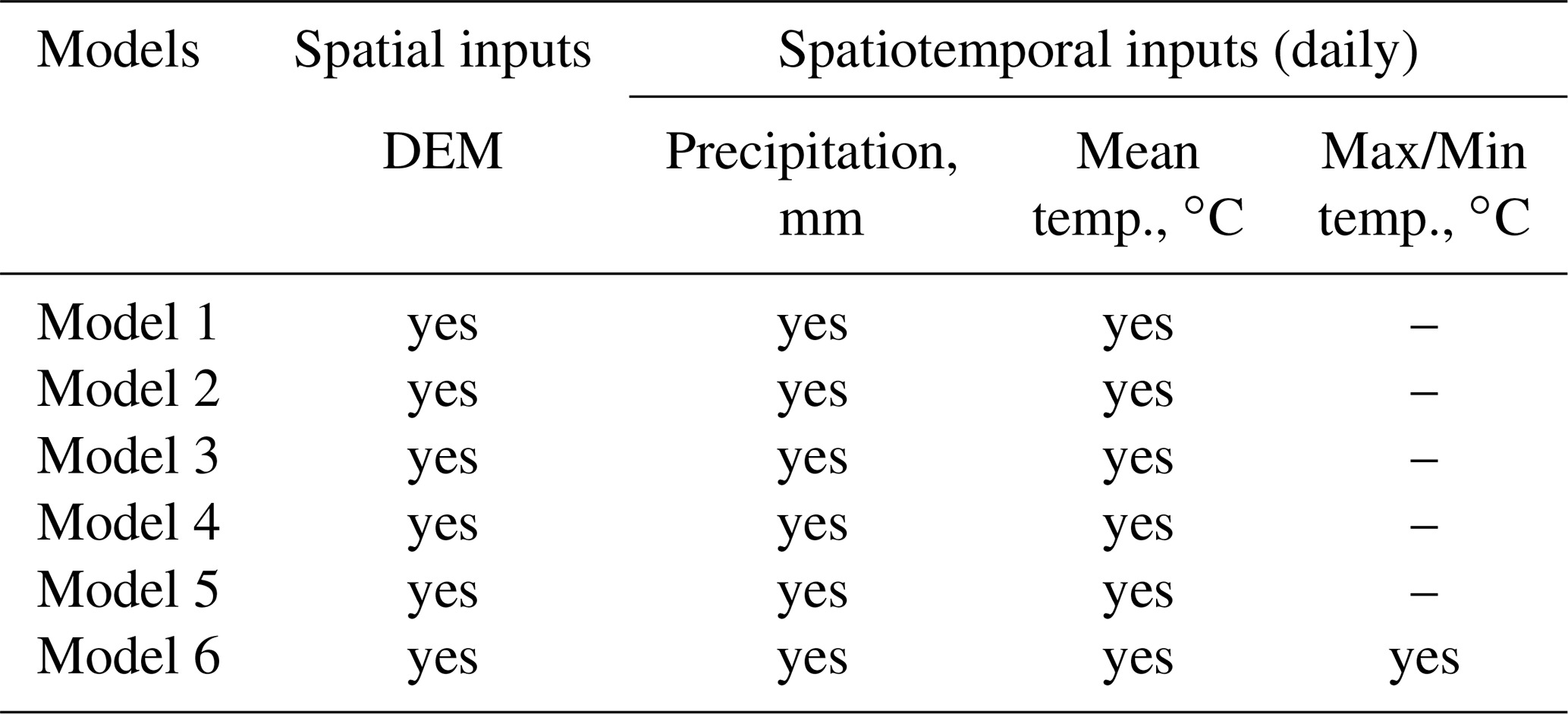
3.2 Data requirement of the models
Table 2 summarizes the input data requirement for each model. The major inputs are the DEM, precipitation, and temperature. The other variables are the derivatives from these major inputs. For instance, daily temperature difference was considered a proxy for the cloud information. The aspect information and daily global radiation are derived from the DEMs. In addition to the data presented in the table, the daily MODIS snow-cover distribution is also required for model calibration and evaluation. Freely available inputs such as the DEM and the MODIS images provide a crucial flexibility with minimum data requirement to drive the snowmelt models. Likewise, daily observed streamflows are also used for calibration and validation of the HBV model.
3.3 Model calibration
The model calibration in this study was done in two distinct steps. Firstly, the six aforementioned snowmelt model variants were calibrated using snow-cover distributions. The second calibration step was done for two hydrological models, namely, the original HBV (Bergström, 1995), henceforth termed “standard HBV”, and a HBV model modified to accommodate the standalone melt outputs from the best-performing snow-routine variant as inputs, from henceforth termed “modified HBV”. In order to calibrate the snow model parameters, the snow cover simulated by the snow model was compared with the MODIS observations on selected days or periods with available data. A pixel was considered snow covered if the simulated snow water equivalent exceeded a preconsidered snow water equivalent threshold of 0.5 mm which corresponds to a snow depth of approximately 2.5 mm.
The calibration is based on the Brier score (BS) (Eq. 9). It is a score function that measures the accuracy of probabilistic predictions. The BS in this study refers to the mean squared error between observed binary patterns of snow/no snow from MODIS and the ones simulated by the extended degree-day models. The Brier score varies between 0 and 1 with the values closer to 0 indicating better agreement between the model outputs and the MODIS image.
where fi(t)= simulated snow-cover (0/1) on day t and pixel i, oi(t)= observed snow-cover (0/1) on day t and pixel i
The objective function is the sum of the BS values over the days with observed MODIS snow-cover:
where tk are the days with observed MODIS snow-cover.
The snow model parameters were identified by minimizing objective function in Eq. (10). In order to reflect the equifinality imparted by the model, the Robust Parameter Estimation (ROPE) methodology was applied for the model parameter optimization. ROPE uses the concept of data depths to identify best-performing robust parameter sets and their properties for different calibration periods in different catchments, with an underlying assumption that it identifies parameter sets without overemphasizing the processes defined by the parameters. Further details regarding ROPE can be found in Bárdossy and Singh (2008). For the calibration, the following steps were carried out.
-
The bounds for the model parameters were set.
-
N random parameter sets (XN) were generated in d dimensions of space limited by the bounds set in Step 1.
-
The models (snowmelt, standard HBV and the modified HBV) were run for each parameter sets and the corresponding objective functions were calculated.
-
Based on the model performance, a predefined subset of the best-performing parameter sets were drawn.
-
2⋅N random parameter sets were again generated within the bounds of the best-performing sets from Step 3.
-
A set of YM parameters were identified where for each vector θϵYM, the depth calculated with respect to the subset is greater than 0, i.e., D(θ)>0.
-
Within the bounds defined by the “deep” parameter sets in Step 6, further “N” parameter sets were generated so that XN=YM.
-
Steps 3–6 were repeated for various iterations assuming that the performance corresponding to YM does not differ more than what one would expect from the observation errors.
A set of 1000 heterogeneous parameter vectors with similar model performance in terms of the objective function were generated. These sets of “good” points can be defined as the parameter sets that are less sensitive and transferable, thereby providing a “compromised” solution. These parameter vectors were estimated for each region by assuming a spatiotemporally constant or variable (wherever possible) parameter distribution and were estimated within a plausible range as described in different snow modeling studies.
ROPE was applied to calibrate the snowmelt models, the standard HBV model with snow, and the modified HBV with external melt for this study. For the snowmelt models, the calibration was initially done for both regions on daily snow-cover images with more than 60 % valid pixels (< 40 % cloud cover) for the snow season in different years. The snow season was selected as October–May for Baden-Württemberg and September–June for Switzerland, assuming a possible snow cover being present for the time period. The second calibration was the hydrological calibration with discharge data at the catchment level and was done for the whole years of 2011–2015 in Baden-Württemberg and 2011–2018 in Swiss catchments with 2010 as the warm-up year. Here, the modified HBV had the melt from the selected snowmelt model as standalone input. The discharges simulated by the standard HBV and the modified HBV were compared for each of the catchments. The Nash–Sutcliffe efficiency (NSE, Eq. 11) was used to evaluate the performance of the melt inputs, where the simulated and observed variables refer to modeled and observed discharge at time t.
where
-
simulated variable at time t,
-
observed variable at time t,
-
mean of observed variable for the time period T,
-
T= length of time series.
3.4 Model validation
The calibrated parameter vectors were used to validate the simulated snow patterns for different seasons using the sets of MODIS images representative of the season as well as for individual images representing unique isolated events, for both BW and Switzerland. To analyze the performance of the snow models at a catchment level and subsequently for the discharge evaluation, five catchments were selected (viz. Neckar at Horb and Rottweil in BW and Reuss at Seedorf, Thur at Andelfingen, and Aare at Brienzwiler in Switzerland). At the catchment level, the snow routine parameters from the 1000 best parameter sets of the standard HBV model calibrated on discharge were subset and used to simulate the snow distribution in all the catchments for the same time period. The corresponding Brier scores were calculated. The validation was then done as a comparison of the Brier scores calculated from the 1000 best parameters for the selected snowmelt model calibrated on MODIS images (for each catchment) and the 1000 best Brier scores obtained from the snow routine of the standard HBV model calibrated on discharge. To validate the performance of melt outputs from the snow-cover calibrated snowmelt models, the 1000 best NSE values from the standard HBV model and the modified HBV model, both calibrated on discharge for the same calibration period for all five catchments were compared. The evaluation was assessed based on the ranges and dispersion of the two sets of best NSE values.
3.5 Model uncertainty
A common problem of hydrological modeling is that, due to the inaccurate observations and simplified representation of the relevant hydrological processes, the parameters of the models cannot be identified accurately. Due to this equifinality, a set of acceptable model parameters can be assessed. If one can use specific additional information, the set of acceptable model parameters may reduce, leading to uncertainty reduction. In the case of snow modeling, the parameters of a hydrological model can be split into two distinct parts: the snow accumulation and melt parameters θs and the other model parameters θm. If the snow model parameters θs are calibrated independently of the model parameters, θm, one receives a parameter set Ms – as the same problem of equifinality occurs for the snow models too. For each θs∈Ms, one can calibrate the hydrological model parameters θm leading to a set Mm. This way, a well-performing parameter set can be obtained. However if the parameters of the model θm are such that the model quality is the same as for calibrating the parameters (θs,θm) by jointly (without using snow observations) obtaining the parameter set M, then the parameter set . This is because all parameter combinations in Msm could also be obtained from the traditional model calibration, but there are parameters in M where parameter compensations lead to snow parameters θs which are not acceptable for the snow model evaluation. Thus, model calibration of the conceptual model may not lead to a better model performance but instead can reduce uncertainty. On the other hand, the separate calibration of the hydrological model and the snowmelt model makes it possible to include more parameters into the snow model. If the same model would be calibrated together with the hydrological model, the increase of the number of parameters would lead to a much more complex calibration procedure. In the results section this is demonstrated for the models considered.
4.1 Model results
4.1.1 Switzerland
For the calibration of the snowmelt model variants, a set of MODIS images for the whole snow season of 1 September 2012 till 30 June 2013 for Switzerland was selected as the reference snow-cover distribution series. The calibration performance values of model variants are expressed in terms of Brier scores as well as confusion matrices depicting the proportion of true and false identifications of snow and no-snow pixels. The overall model error, i.e., the sum of falsely identified instances of snow and no-snow pixels, is the Brier score. Table 3 shows the calibration results of different model variants as normalized confusion statistics calculated for the reference time period for Switzerland. The columns of the confusion statistics table indicate the proportions of true negatives (both “no snow”), false positives (MODIS: “no snow”, simulated: “snow”), true positives (both “snow”), and false negatives (MODIS: “snow”, simulated: “no snow”). All six models reported good Brier scores ranging from 0.084 to 0.095. The results indicate that the models have very close performance when calibrated over the course of a whole snow season in Switzerland. Model 6, with the radiation-induced melt, has the best performance in terms of overall Brier scores as well as the reduction in the false recognition of snow. This model, however, slightly overestimates the snow in the region. Figure 4 shows the validation of the radiation-based model on the snow-cover image for a relatively cloud-free day (8 January 2013). The figure shows that the model calibrated on the whole season adeptly mimics the MODIS snow-cover distribution for the day with a very good Brier score of 0.077. The left plot in the figure is the MODIS image for the reference day, the central plot shows the simulated image for the day, and the right one shows the differences in prediction.
Table 3Normalized confusion matrices for the calibration periods (a) Switzerland for 1 September 2012 till 30 June 2013 (b) Baden-Württemberg for 1 October 2012 till 31 May 2013.
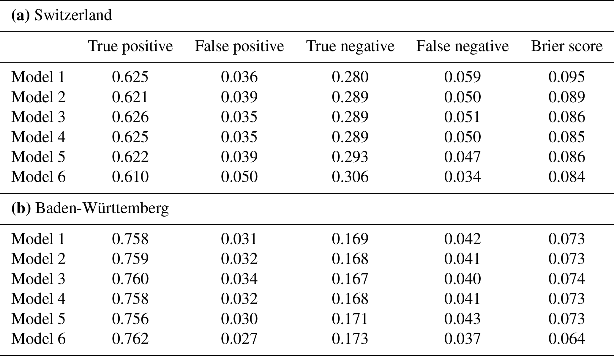
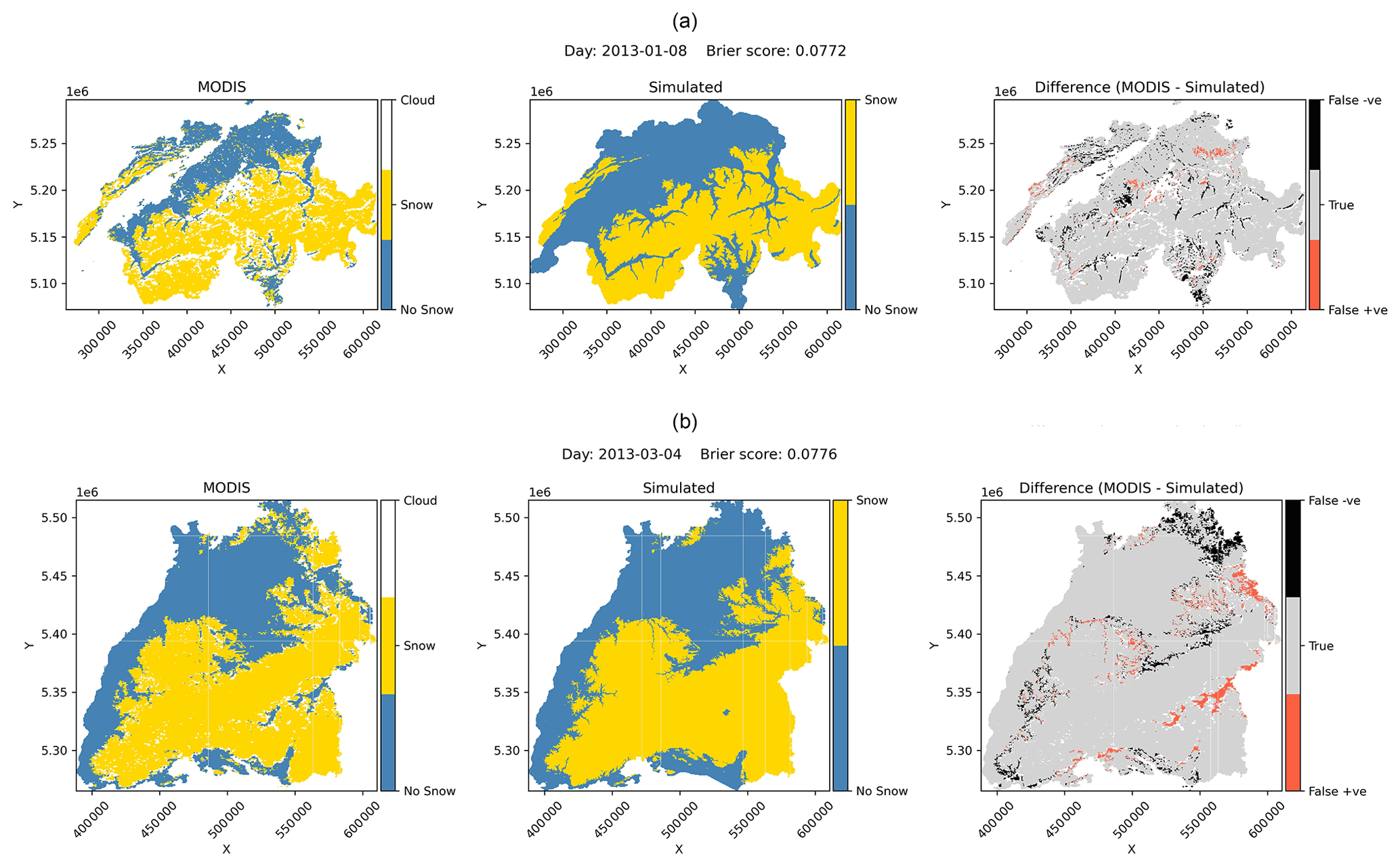
Figure 4MODIS inferred (left) vs. Model 6 simulated snow distribution (center) and differences between MODIS and simulated image (right); (a) Switzerland (b) Baden-Württemberg.
The model performances were further scrutinized in different elevation zones in both regions in terms of underestimation, overestimation, and total estimation errors. Underestimation error is the average normalized false negative instances, overestimation error is the average normalized false positive instances, and total error is the mean Brier scores for each elevation zone. Figure 5 shows the results for Switzerland. Model 6 showed a reduction in overestimation error throughout the elevation zones in comparison to other models. However, the model was underestimating snow for elevations below 1500 m a.s.l. The overall error, however, remains lower for the < 500 and > 2500 m a.s.l. regions. The mean error remained the lowest, implying the best performance among the variants.

Figure 5Model performances in different elevation zones (left: overestimation error, middle: underestimation error, right: total error (Brier score), dashed: mean error for all elevation zones); (a) Switzerland; (b) Baden-Württemberg.
4.1.2 Baden-Württemberg
The different snow models were also tested in this region in Germany. The region was selected to test the efficacy of the approach in a shorter-duration snow region. Here, the snow season of 1 October 2012 till 31 May 2013 was selected as the reference period, and the corresponding MODIS images were used for calibration . As in Switzerland, all models were able to mimic the snow-distribution pattern for the reference day very well. Model 6 outperformed all the other model variants as shown by the proportion of true and false predictions in Table 3. A gradual improvement in model performance with additional parameterization can be inferred from the table. Though comparable, Model 6 Brier scores have a starker contrast with other model results, in comparison to the Swiss results. A good improvement in true recognition and a subsequent reduction in false identification can be observed with the radiation-based model. An illustration of the validation of Model 6 on a cloud-free day of 4 March 2013 can be seen in Fig. 4. The simulated image matches the MODIS image for the day with about 93 % accuracy, which reflects the strength of the seasonal calibration. Likewise, elevation-based discretization of the model performance in Baden-Württemberg, as depicted by Fig. 5, shows that the radiation-based model and Model 1 have the lowest underestimation error. The error, however, increases with increasing elevation. The overestimation error is the lowest for Model 4, and the trend decreases as the elevation increases for all but Model 1. The overall error is highly reduced with Model 6 throughout all elevation zones as indicated by the right panel.
Though all the models perform very well in the overall scenario as well as in all the elevation zones as reflected in the performance scores, Model 6 was selected for both Switzerland and Baden-Württemberg, owing to the lowest overall error, and from here on it is used as the reference model for further analysis.
4.2 Sensitivity analysis of different thresholds for snow/no-snow differentiation
Sensitivity analysis was carried out for different thresholds using the reference model for both Baden-Württemberg and Switzerland to identify the best snow/no-snow differentiation. The time period used for the analysis was from 2013–2015. The thresholds analyzed were the Normalized Difference Snow Index (NDSI) thresholds to demarcate the snow and no-snow pixels in the reference MODIS images; cloud threshold as a percentage of valid pixels to demarcate the number of daily images to be used as a reference series to calibrate against; and the snow detection threshold to define the simulated snow water equivalent (SWE) as a snow pixel in the simulated snow cover distribution. Different NDSI thresholds ranging from 1 to 95, cloud thresholds ranging from 10 % to 90 %, and detection thresholds from 0 to 5 mm were considered for the analysis. A NDSI threshold of 1 means that the MODIS images with pixel value greater than 1 was considered a reference snow pixel. Likewise, a cloud threshold of 10 % indicates that, for a given calibration period, images with less than 10 % cloudy pixels would be selected for calibration. Similarly, a SWE threshold of 0.5 mm would mean that the pixels with simulated SWE above 0.5 mm were considered a simulated snow pixel. The detailed results are presented in the Appendix Figs. A1, A2, and 6.
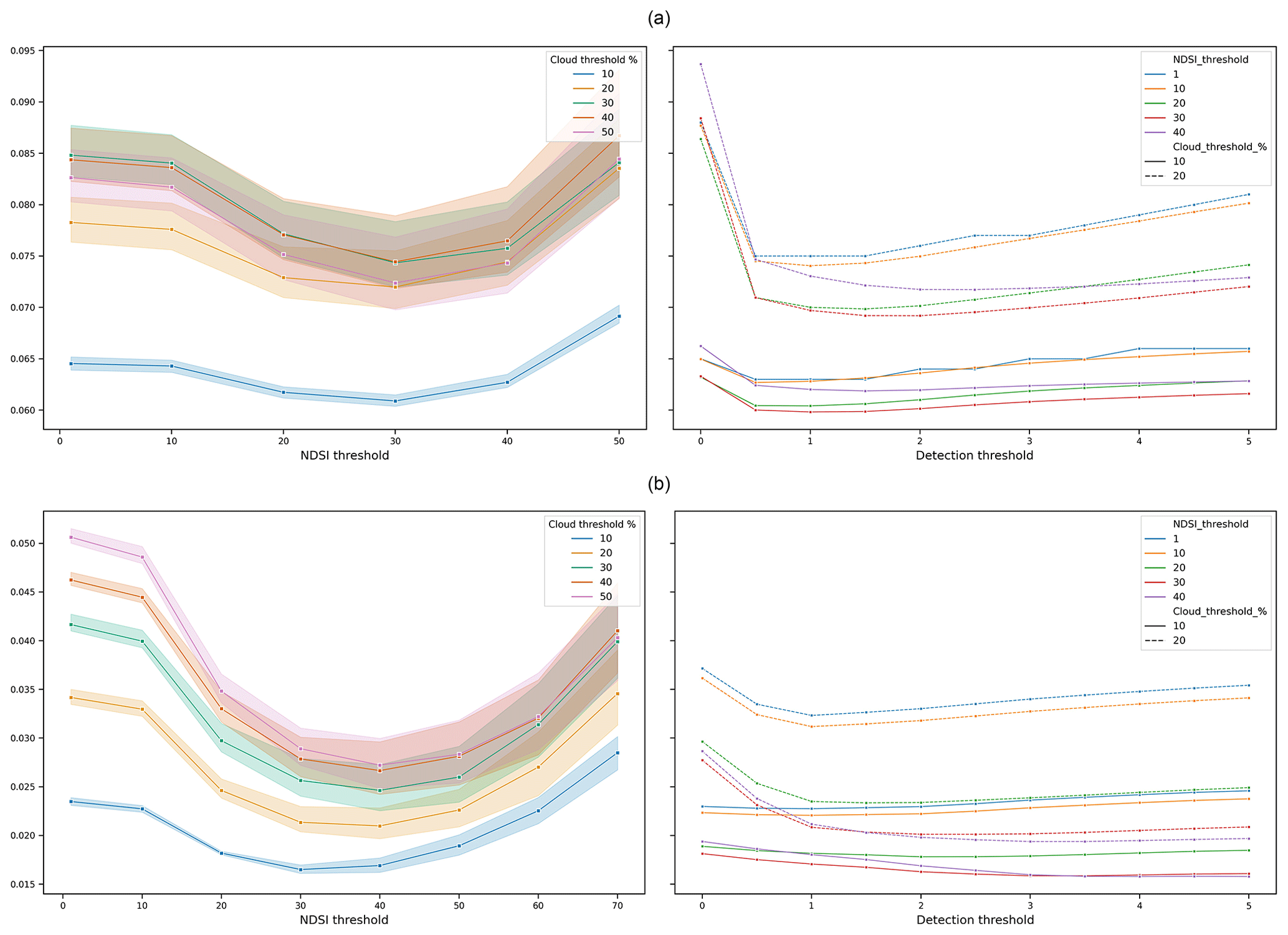
Figure 6Model performance for different thresholds in (a) Switzerland and (b) Baden-Württemberg; left panel: the shaded regions indicate the performance for different SWE thresholds; right panel: solid and dashed lines, respectively, show performance values for 10 % and 20 % cloud thresholds. Detection threshold in the x-axis level refers to the SWE thresholds.
From the figures, it can be clearly inferred that a NDSI threshold of 30, cloud threshold of 10 %, and a SWE threshold above 0.5 mm could achieve the best performance in terms of Brier scores in Switzerland. Likewise, the results for BW show that a SWE detection threshold of 2.0 mm or above, coupled with the NDSI threshold of 30 and a cloud threshold of 10 %, gives the best simulation of the snow cover distribution. The results for both regions are similar to each other, which highlights the applicability of the adopted methodology in different snow regimes.
4.3 Sensitivity analysis on the selection of calibration periods
A sensitivity analysis on the selection of different calibration periods was also carried out for the snow season of 2012–2013. For this, the reference model was calibrated against sets of daily MODIS images representing different stages in a snow season – viz. whole season (September–June for Switzerland and October–May for BW), onset season (September–February for Switzerland and October–February for BW), melt season (March–June for Switzerland and March–May for BW), peak snow month (February for both), and the day with highest amount of cloud-free snow (18 February for Switzerland and 12 February for BW). The thresholds were adopted as per the earlier section (i.e., for BW, NDSI: 30, cloud %: 10, SWE threshold: 2.5 mm; for Switzerland, NDSI: 30, cloud %: 10, SWE threshold: 0.5 mm). The reference model was calibrated for all the aforementioned seasons using the ROPE algorithm. One thousand best parameter vectors were identified for each season. These parameters for each calibrated period were then iteratively checked for whether they were contained within the convex hull defined by the validation parameters to identify the percentage of these contained parameter sets. Subsequently, the calibrated parameters were validated for each season to analyze the temporal transferability of the parameter vectors and identify the best calibration set that would work well with all the seasons/periods. Figure 7 presents the validation of calibrated parameters in different seasons. This validation is expressed as the percentage of the reference parameter vectors for each season/period contained by the hull defined by the validation parameter sets for Baden-Württemberg and Switzerland, respectively. The figures indicate that the calibrated parameters for the whole season work well for different validation periods in both regions, with a relatively higher containment of the calibration parameters in reference to the validation sets. In Switzerland, the melt season calibration exhibits a better temporal transferability as indicated by the higher proportions of the parameter vectors in each season, whereas in Baden-Württemberg the onset season calibration shows higher transferability of the parameters. Based on these results, it was concluded that the melt season calibration in Switzerland and the onset season calibration in Baden-Württemberg imparted more robust parameter sets for both study areas. The whole season calibration showed good agreement with other periods in both regions. Figure 8 provides a better understanding of the Brier score dispersion for the regions for these selected calibration periods. In Baden-Württemberg, the onset season calibration is well validated for the peak snow season and the single-day event. The melt season calibration is also comparable with the onset season performance. The whole season calibration has better performance for onset and melt seasons but with a more uncertain validation for the peak snow month and single-day image, as shown by the boxplot bounds. In Switzerland, melt season calibration shows a better validation for almost all the seasons. This indicates that the images available towards the end of the season can simulate the whole snow season very well. However, the seasonal calibration performance remains similar as in the case of Baden-Württemberg.
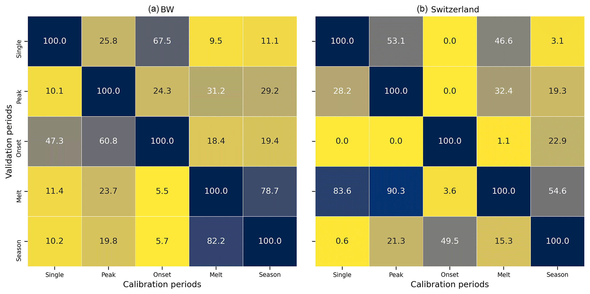
Figure 7Percentage of calibrated parameter sets contained by the convex hull defined by the validation parameter sets.

Figure 8Model performance in the validation periods (a) Switzerland (left panel: validation results for melt season calibrated parameters, right panel: validation results for whole season calibrated parameters) and (b) Baden-Württemberg (left panel: validation results for onset season calibrated parameters, right panel: validation results for whole season calibrated parameters); x-axis labels “calib.”: calibration performance for the same season, “valid.”: validation performance using the reference season parameters.
4.4 Snowmelt model results at catchment level
The reference snowmelt model (Model 6) was also calibrated for two catchments in Baden-Württemberg and three in Switzerland on snow-cover distribution for the winter season throughout 2010–2015 (BW) and 2010–2018 (Switzerland). ROPE was used to calibrate the models and obtain 1000 sets of best-performing parameter vectors for each catchment, based on the overall Brier scores. The simulated snow-cover distribution was compared with the ones estimated by the HBV's snow routine to assess the representation of snow accumulation and melt processes within. The 1000 HBV snow parameter sets were subsetted from the best-performing parameter vectors obtained during ROPE calibration of the HBV model on discharge for each catchment. The comparison results are shown in Fig. 9. It is evident from the violin plots that the snowmelt models clearly outperform the HBV snow routine in all catchments while estimating the snow-cover distribution estimation. The median Brier score values for the snowmelt models in all catchments are lesser than their counterparts. Moreover, the 1000 best Brier score values for the snowmelt models depict a very narrow spread in contrast to a much wider spread from the HBV's snow routine. This shows the uncertainty of the HBV during the simulation of snow accumulation and melt, which hints towards a compensating effect with other non-snow parameters. This spread is more pronounced in the Horb and Rottweil catchments, which are characterized by shorter-duration snow. The results suggest that HBV's snow routine, when calibrated on discharge together with the other model parameters, is not able to capture the snow dynamics in the BW region as compared to the spread in Swiss catchments with longer-duration snow. This approach thus adds value to these regions as the calibrated snow-cover distribution provides a strong basis for estimating available water coming from snow, as these regions are dependent on the melt waters. The results thus strongly indicate that the use of a standalone snowmelt model, in this study, provides a very stable and reliable representation of the snow-cover distribution and in turn the melt.
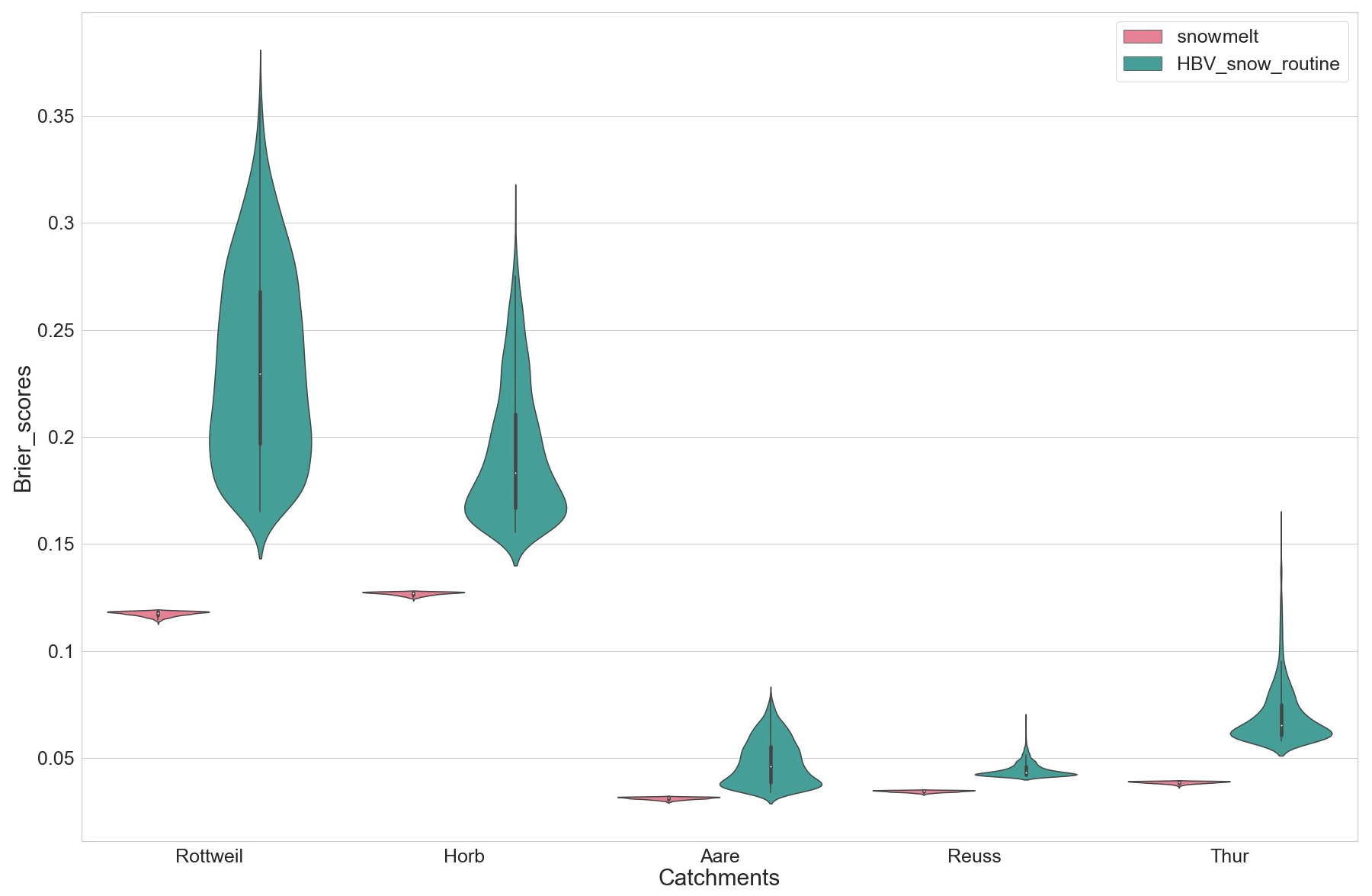
Figure 9Violin plots comparing the performance of the reference snowmelt model in different catchments and HBV's snow routine in terms of Brier scores. The height of the violin plots shows the range of Brier scores whereas the shape of the curve depicts their density.
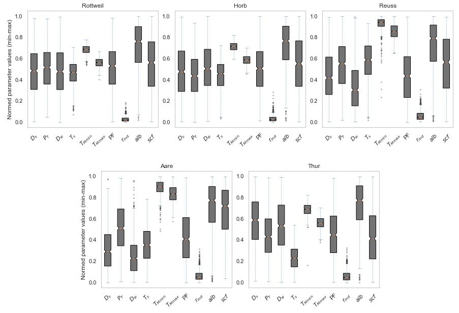
The boxplots showing the dispersion of the parameters are shown in Fig. 10. The y axis shows the normalized parameter values based on their min–max range set for optimization. The boxplots indicate that (apart from the radiation melt factor, rind, TMmax, TMmin, and to some extent TS) all the parameter ranges are relatively stable and less sensitive to the model performance. These four parameters are, however, constrained by the objective function, and it is understandably so, because these parameters are more sensitive as they govern the appearance and disappearance of the snow.
4.5 Validation in hydrological models
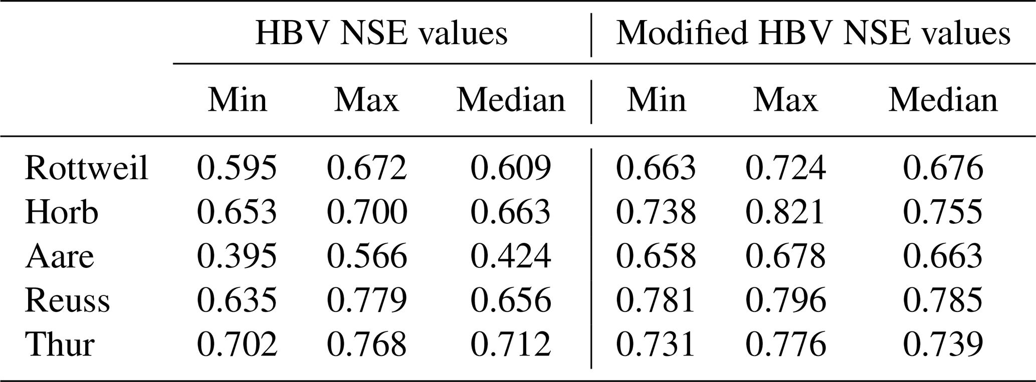
The best-performing parameter vector from the snowmelt models for each catchment was used to simulate the melt waters exiting the snow regime, which was, in turn, used in the modified HBV model to simulate the hydrologic implications of the melt as a standalone input. The modified HBV was calibrated on discharge for the whole time series for each of the catchments. This was done with three iterations of ROPE. The standard HBV was also calibrated on the same discharge data but with five ROPE iterations. With the ROPE calibration, 1000 robust parameter sets were identified for both hydrological models. The best NSE values were subsequently compared to assess the performance of the snowmelt models against the HBV. The results are shown in Fig. 11 and Table 4. The results show that the addition of melt improves the hydrological model performance in each of the catchments, notably in the snow dominated ones in Reuss and Aare. The median NSE values show improvement in all of the catchments in the study domain. The NSE spread is also smaller in the case of modified HBV. This highlights uncertainty reduction, as the hull containing the equifinal parameter vectors becomes smaller as a result of lesser parameters to calibrate for the modified HBV variant. The results suggest that the improvement in model performance comes with a better computational efficiency and a better “mimicry” of the snow accumulation and melt.

Figure 11Performance comparison of the standard and the modified HBV models in terms of NSE in different catchments. The shape of the violin plots indicates the density plots for the 1000 best NSE values for each model.
It is a big challenge and a highly imperative one to improve the snowmelt routines in widely and successfully tested rainfall–runoff models like HBV (Bergström, 2006; Girons Lopez et al., 2020). In this milieu, to evaluate the snow processes based on spatial distribution of snow, we implemented an image-based pattern calibration approach using MODIS-inferred snow-cover distribution for a single day or a duration of snow season of a given year. The calibration was done based on pixel-based binary information (“1”:“snow”, “0”:'`no snow”) from the MODIS images in Switzerland and Baden-Württemberg. The MODIS data, available freely across the world and at a daily resolution, provide a plausible alternative to ground-based data for immediate verification of snowmelt models. Widely used and computationally simplistic temperature index models with low data requirements were considered in the study and were modified wherever possible to gain enhanced model performance.
We found that all the model variants calibrated on a set of individual snow-cover images for the whole season were able to track the MODIS snow distribution with very good accuracy. These models were evaluated based on a Brier score which represents the total false recognition of snow and no-snow pixels. Results from all the models are comparable and very close in simulating the snow-cover distribution. The models' performance in terms of overestimation, underestimation, and total estimation errors were further scrutinized in different elevation zones. We observed that for Switzerland, characterized by the longer-duration snow, all the models were found to show decreasing overestimation error with increasing elevation, except Model 6 where the model error slightly increases in the mid-elevation zones. However, the model performances in terms of underestimation errors tend to increase with higher elevations. We found that the mean overall error remained the lowest for Model 6 with the radiation component for Switzerland. In Baden-Württemberg, the overall error is the lowest for all elevation zones with the radiation-based model. While some of the model variants were able to track the snow-cover distribution with better accuracy, we did not find a model-specific clear trend of prediction errors in different elevation zones. Based on the mean performance, Model 6 was deemed accurate enough to simulate the snow-cover distribution with a higher accuracy in identifying snow and no-snow pixels, reflected on the low Brier score values. As a reference model for further analysis, we selected this relatively complex variant with daily potential clear-sky radiation for both regions. The inclusion of radiation-induced melt has been found to provide a more realistic spatial distribution of melt rates (Hock, 1999). However, it is to be noted that since this approach is flexible enough to work with different snowmelt modules which can simulate the snow-cover distribution, we selected the relatively complex radiation-based model to assess the added value of the robust binary data selected for calibration purpose.
We also carried out a sensitivity analysis on the different thresholds used in the study to differentiate between the snow and no-snow pixels. We found out that a NDSI threshold of 30, a cloud percentage threshold of 10 %, and a SWE threshold of above 2.0 mm perform with very good accuracy for a seasonal calibration where all MODIS images fitting the cloud threshold criteria are used to calibrate the models in both regions. A closer look into the analysis suggests that, for Baden-Württemberg, NDSI thresholds of 30 and 40 give similar results when the SWE threshold of higher than 2.0 mm is used with 10 % cloud thresholds. In Switzerland, NDSI threshold of 30 showed the best performance with SWE thresholds higher than 0.5 mm. However, it is to be mentioned that this analysis was done assuming MODIS as the observed snow-cover distribution. Earlier studies on the NDSI thresholds (Tong et al., 2020; Härer et al., 2018) have suggested that a threshold of 40 can be used for robust estimates of snow cover from MODIS. However, in reality, the spatial detail of MODIS and the associated uncertainty (Tong et al., 2020) make it harder to know where the snow actually is. Coupled with this is the uncertainty associated with the precipitation data. These added uncertainties make it harder to recommend a definite threshold for future applications. The adopted calibration technique was found to be more sensitive towards the NDSI threshold, particularly in Switzerland, as can be observed from Appendix Fig. A1. In contrast, Appendix Fig. A2 shows that the sensitivity to NDSI is not that significant in Baden-Württemberg. It is thus our observation that a NDSI threshold of 20–50 can be considered to demarcate the snow/no-snow information for MODIS-based snowmelt simulations, along with a SWE threshold of 0.5–5 mm for longer-duration snow conditions and 2–5 mm for relatively shorter-duration snow conditions, without much loss in model performance. Nester et al. (2012) have also identified a SWE thresholds of 2.5 mm as optimum for error analysis with MODIS SCA. A cloud detection threshold of 10 % was found to be the ideal threshold for the selection of MODIS images for calibration, although our methodology is not that sensitive in terms of cloud coverage as can be seen in the appendix figures. This highlights the fact that this calibration on binary pixel information can also be done on patches of snow-covered pixels free from clouds, which makes this approach very flexible. However, different studies have found cloud threshold to be a critical factor during the evaluation of model errors. Şorman et al. (2009) adopted a cloud threshold of 20 % for a multi-variable hydrological model calibration. Nester et al. (2012) suggested a cloud threshold of 80 % as there were no significant differences in model errors for < 50 % and 50 %–80 % cloud cover in their study.
The sensitivity analysis on the selection of dates of the MODIS images for calibration showed that the selection of the dates has a very strong impact on the model performance and in turn on transferability of parameters. The melt season calibration in Switzerland and the onset season calibration in Baden-Württemberg were found to have the best validation in other seasons and periods. With a more clearly defined melt season in Switzerland, we found out that the images towards the end of the snow season were adequate enough to simulate the snow processes within the snow season with good accuracy, and these calibrated parameters were found to be robust as shown by the spread of Brier scores in the validation periods (refer Fig. 8). However, in Baden-Württemberg, which is characterized by a distinct onset but a more uncertain melt season (lesser snow availability), the onset season calibration was observed to be more robust and transferable to other validation periods. On a catchment level, three catchments in Switzerland and two in Baden-Württemberg were selected. The snowmelt model was calibrated using multiple images for winter seasons throughout the time period to obtain a set of 1000 robust parameter vectors. The temperatures demarcating snow and melt onset and the radiation melt factor were deemed sensitive to the overall Brier scores. The Brier scores from these 1000 simulations were compared with the ones estimated with parameters in the HBV's snow routine. The calibrated snow model significantly outperforms the HBV's snow model calibrated on discharge in all of the catchments. This has also been discussed by Udnæs et al. (2007) and Parajka and Blöschl (2008) in their respective studies showing that calibration on SCA in addition to runoffs improved the snow model efficiency. Furthermore, our results clearly show that the uncertainty in simulation of the snow-cover distribution is significantly reduced when using a dedicated snowmelt model, as the snow parameters in the HBV calibrated on discharge are compensated with other non-snow parameters. This compensation leads to a more uncertain representation of the snow accumulation and melt dynamics. This decrease in uncertainty with a simplified calibration approach using freely available data is noteworthy as the calibrated parameter vectors are more robust as compared to the ones calibrated on discharge. Similar findings have been pointed out by Riboust et al. (2019), where they discussed the increased robustness of the snow model parameters when SCA was added to the calibration. Since this methodology implements the calibration at pixel level on binary (“snow”, “no-snow”) information instead of depths, relatively complex snowmelt models are also calibrated with more robustness and without over-calibration of the models. This can be attributed to the robust data selected for calibration and the spatial extent of the satellite images used for simulation. It is to be noted that this study does not intend to assess the performance of any specific hydrological model predictions; however, it does aim to assess the performance of the melt outputs of snowmelt models calibrated on snow-cover distribution in a basic hydrological model. We deem it important to point out that though two of the Swiss catchments, Aare and Reuss, are glaciated, the glacial melt was not taken into account. This was mainly because of the MODIS limitation to identify the glaciers (Muhammad and Thapa, 2020) and to avoid further parameterization of the hydrological model to include a glacier component. Since our aim is to evaluate the snowmelt model calibration, both hydrological models were calibrated on equal terms with a similar approach with results comparable to each other. We found good improvement in the NSE performance in all the catchments while using the modified HBV. Parajka and Blöschl (2008) also concluded that the median runoff model efficiency increased when MODIS data were used for the calibration in comparison to a traditional discharge calibration. Bennett et al. (2019) concluded in a similar tune with their results showing MODIS fractional snow-covered area (fSCA) improving the internal snow timings as well as the hydrological simulations. Our results further show that the NSE dispersion is also reduced with the modified HBV simulations, indicating a reduction in model uncertainty as both sets of parameters required for calibration as well as the set of equifinal parameters become smaller. This gain in performance comes with better computational efficiency, as the modified HBV calibration converges faster. This allows for incorporation of additional parameters in the independent snowmelt models to better represent the snow dynamics, as opposed to the fact that additional parameters in hydrological models impose further complexity during calibration. With a dedicated snowmelt model, this can be achieved as it is relatively quicker to calibrate on the images, and the resulting melt can be used in the hydrological models for efficient calibration. Di Marco et al. (2021) also concluded that a combination of MODIS fractional snow-cover area and streamflow data led to a reduction of predictive uncertainty of a hydrological model, thereby leading to sharper and reliable flow simulations. Furthermore, the strength of this approach lies in the simplicity, spatial flexibility, and global availability of the model input data, which can be very useful for snowmelt and hydrological predictions in data-scarce regions.
The study presented a methodology to evaluate a daily MODIS snow-cover-based calibration in identifying distribution patterns of snow in snow-dominated regimes in Switzerland and Baden-Württemberg (Germany). Specifically, different model modifications were employed to assess the improvement in the simulation of snow distribution with lesser input requirements. By calibrating at pixel level on binary information, relatively complex snowmelt modules can be calibrated with more robustness, as the uncertainty associated with calibration data is reduced, as is often the case with calibrations based on snow depth or snow water equivalent. From our results, we can conclude the following:
- a.
It was observed that the methodology does well in mimicking the snow-cover distribution in regions with relatively higher accuracy with all the models.
- b.
For the study regions, NDSI thresholds and SWE thresholds for snow/no-snow differentiation, respectively, for the MODIS and simulated snow distribution were identified along with the best cloud percentage threshold option critical for the selection of MODIS images for calibration.
- c.
Depending on the snow regimes, the results suggest that a set of MODIS images within a period during the snow season are adequate to adeptly simulate the snow-cover distribution for the whole season.
- d.
Comparison of the snowmelt model's performance with the HBV's snow routine shows that the uncertainty in the representation of snow accumulation and melt processes can be reduced with a standalone calibration of a snowmelt model, as HBV calibration on discharge usually exhibits a compensating behavior with other non-snow parameters. The improvement in model performance can be deemed for “a right reason” with a better representation of the underlying snow processes.
- e.
The calibration using readily available images used in this method offers adequate flexibility, albeit with simplicity, to calibrate snow distribution in mountainous areas across a wide geographical extent with reasonably accurate precipitation and temperature data, especially in data-scarce regions, with parameters estimated with MODIS. The other data used for the snow models can be derived from publicly available digital elevation models.
The reduction in model uncertainties, primarily with the snow-distribution estimation and with the discharge simulation, adds value to provide improved conceptualization of the temperature-index model routines and further potential model updating in future work. Furthermore, this approach is not dependent on the choice of hydrological model, as it can be extended to any hydrological model that can identify the snow-cover distribution.
A1 Switzerland

Figure A1Sensitivity analysis results for NDSI, cloud percentage, and SWE thresholds in Switzerland; detection threshold in the figure refers to the SWE thresholds.
A2 Baden-Württemberg
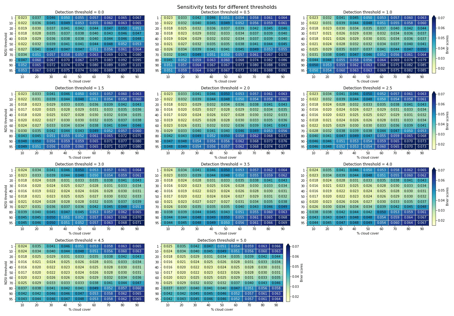
Figure A2Sensitivity analysis results for NDSI, cloud percentage, and SWE thresholds in Baden-Württemberg; detection threshold in the figure refers to the SWE thresholds.
Codes for the snowmelt models and the model evaluation are available at https://doi.org/10.5281/zenodo.6549342 (Gyawali, 2022). The codes for the ROPE-based optimization scheme can be explored from https://github.com/faizan90/depth_funcs (Anwar, 2020).
The precipitation and temperature data were obtained from the Climate Data Center of the German Weather Service (https://opendata.dwd.de/climate_environment/CDC, DWD, 2021) and the Swiss Federal Office of Meteorology and Climatology (https://gate.meteoswiss.ch/idaweb, MeteoSwiss, 2020). The MODIS snow-cover images were downloaded using the Earthdata Search tool (https://search.earthdata.nasa.gov/search, see also Hall and Riggs, 2016). The DEM was obtained from https://srtm.csi.cgiar.org/srtmdata/ (last access: 18 February 2018, see also Jarvis et al., 2008).
This study is a part of DG's doctoral research which is supervised by AB. The study was conceptualized by AB and DG, and it was implemented by DG. Both authors contributed to the writing, reviewing, and editing of the paper.
At least one of the (co-)authors is a member of the editorial board of Hydrology and Earth System Sciences. The peer-review process was guided by an independent editor, and the authors also have no other competing interests to declare.
Publisher's note: Copernicus Publications remains neutral with regard to jurisdictional claims in published maps and institutional affiliations.
The authors would like to thank Juraj Parajka, one anonymous reviewer, and Bettina Schaefli for taking their time to provide critical, constructive, and comprehensive comments which helped to improve this paper. The authors further acknowledge Faizan Anwar for his coding support for the ROPE implementation. The authors would also like to acknowledge Deutscher Akademischer Austauschdienst (DAAD) for the doctoral research scholarship which encompasses this study.
This open-access publication was funded by the University of Stuttgart.
This paper was edited by Markus Hrachowitz and reviewed by Juraj Parajka, Bettina Schaefli, and one anonymous referee.
Anwar, F.: Robust Parameter Optimization (ROPE) routine, GitHub [code], https://github.com/faizan90/depth_funcs (last access: 12 December 2021), 2020. a
Bárdossy, A. and Pegram, G.: Interpolation of precipitation under topographic influence at different time scales, Water Resour. Res., 49, 4545–4565, https://doi.org/10.1002/wrcr.20307, 2013. a
Bárdossy, A. and Singh, S. K.: Robust estimation of hydrological model parameters, Hydrology and Earth System Sciences, 12, 1273–1283, https://doi.org/10.5194/hess-12-1273-2008, 2008. a
Bárdossy, A. and Singh, S. K.: Robust estimation of hydrological model parameters, Hydrol. Earth Syst. Sci., 12, 1273–1283, https://doi.org/10.5194/hess-12-1273-2008, 2008. a
Bennett, K. E., Cherry, J. E., Balk, B., and Lindsey, S.: Using MODIS estimates of fractional snow cover area to improve streamflow forecasts in interior Alaska, Hydrol. Earth Syst. Sci., 23, 2439–2459, https://doi.org/10.5194/hess-23-2439-2019, 2019. a
Bergström, S.: Experience from applications of the HBV hydrological model from the perspective of prediction in ungauged basins, IAHS-AISH publication, 97–107, 2006. a
Bergström, S.: The HBV model, in: Computer Models of Watershed Hydrology, edited by: Singh, V. P., Water Resources Publications, Colorado, USA, 443–476, ISBN 978-0-91833-491-6, 1995. a
Beven, K.: How far can we go in distributed hydrological modelling?, Hydrol. Earth Syst. Sci., 5, 1–12, https://doi.org/10.5194/hess-5-1-2001, 2001. a
Caicedo, D. R., Torres, J. M. C., and Cure, J. R.: Comparison of eight degree-days estimation methods in four agroecological regions in Colombia, Bragantia, 71, 299–307, https://doi.org/10.1590/S0006-87052012005000011, 2012. a
Climate Data Center of the German Weather Service (DWD): Index of /climate_environment/CDC/, Deutscher Wetterdienst [data set], https://opendata.dwd.de/climate_environment/CDC, last access: 15 February 2021. a
Debele, B., Srinivasan, R., and Gosain, A.: Comparison of Process-Based and Temperature-Index Snowmelt Modeling in SWAT, Water Resour. Manag., 24, 1065–1088, https://doi.org/10.1007/s11269-009-9486-2, 2009. a
Di Marco, N., Avesani, D., Righetti, M., Zaramella, M., Majone, B., and Borga, M.: Reducing hydrological modelling uncertainty by using MODIS snow cover data and a topography-based distribution function snowmelt model, J. Hydrol., 599, 126020, https://doi.org/10.1016/j.jhydrol.2021.126020, 2021. a
Feng, X., Sahoo, A., Arsenault, K., Houser, P., Luo, Y., and Troy, T. J.: The Impact of Snow Model Complexity at Three CLPX Sites, J. Hydrometeorol., 9, 1464–1481, https://doi.org/10.1175/2008JHM860.1, 2008. a
Franz, K. J. and Karsten, L. R.: Calibration of a distributed snow model using MODIS snow covered area data, J. Hydrol., 494, 160–175, https://doi.org/10.1016/j.jhydrol.2013.04.026, 2013. a, b
Gafurov, A. and Bárdossy, A.: Cloud removal methodology from MODIS snow cover product, Hydrol. Earth Syst. Sci., 13, 1361–1373, https://doi.org/10.5194/hess-13-1361-2009, 2009. a, b
Girons Lopez, M., Vis, M. J. P., Jenicek, M., Griessinger, N., and Seibert, J.: Assessing the degree of detail of temperature-based snow routines for runoff modelling in mountainous areas in central Europe, Hydrol. Earth Syst. Sci., 24, 4441–4461, https://doi.org/10.5194/hess-24-4441-2020, 2020. a, b, c, d
Gyawali, D. R.: Distributed snow-melt model variants, Zenodo [code], https://doi.org/10.5281/zenodo.6549342, 2022. a
Hall, D. K. and Riggs, G. A.: MODIS/Terra Snow Cover Daily L3 Global 500m SIN Grid, Version 6, NDSI_Snow_Cover, Boulder, Colorado USA, NASA National Snow and Ice Data Center Distributed Active Archive Center [data set], https://doi.org/10.5067/MODIS/MOD10A1.006, 2016 (downloaded using Earth Data Search Tool, https://search.earthdata.nasa.gov/search, last access: 19 February 2021). a, b
Hall, D., Salomonson, V., and Riggs, G.: MODIS/Terra Snow Cover 5-Min L2 Swath 500 m, Version 5, Boulder, Colorado, USA, NASA National Snow and Ice Data Center Distributed Active Archive Center [data set], https://doi.org/10.5067/ACYTYZB9BEOS, 2006. a
Härer, S., Bernhardt, M., Siebers, M., and Schulz, K.: On the need for a time- and location-dependent estimation of the NDSI threshold value for reducing existing uncertainties in snow cover maps at different scales, The Cryosphere, 12, 1629–1642, https://doi.org/10.5194/tc-12-1629-2018, 2018. a
He, Z. H., Parajka, J., Tian, F. Q., and Blöschl, G.: Estimating degree-day factors from MODIS for snowmelt runoff modeling, Hydrol. Earth Syst. Sci., 18, 4773–4789, https://doi.org/10.5194/hess-18-4773-2014, 2014. a
Hock, R.: A distributed temperature-index ice- and snowmelt model including potential direct solar radiation, J. Glaciol., 45, 101–111, https://doi.org/10.3189/S0022143000003087, 1999. a
Hock, R.: Temperature index melt modelling in mountain areas, J. Hydrol., 282, 104–115, https://doi.org/10.1016/S0022-1694(03)00257-9, 2003. a, b
Hofierka, J. and Suri, M.: The solar radiation model for Open source GIS: implementation and applications, Proceedings of the Open source GIS – GRASS users conference, 2002. a
Hudson, G. and Wackernagel, H.: Mapping temperature using kriging with external drift: Theory and an example from scotland, Int. J. Climatol., 14, 77–91, https://doi.org/10.1002/joc.3370140107, 1994. a
Jarvis, A., Reuter, H. I., Nelson, A., and Guevara, E.: Hole-filled seamless SRTM data V4, International Centre for Tropical Agriculture (CIAT) [data set], https://srtm.csi.cgiar.org (last access: 18 February 2018), 2008. a, b
Kirkham, J. D., Koch, I., Saloranta, T. M., Litt, M., Stigter, E. E., Møen, K., Thapa, A., Melvold, K., and Immerzeel, W. W.: Near Real-Time Measurement of Snow Water Equivalent in the Nepal Himalayas, Front. Earth Sci., 7, 177, https://doi.org/10.3389/feart.2019.00177, 2019. a
Liu, T., Willems, P., Feng, X. W., Li, Q., Huang, Y., Bao, A. M., Chen, X., Veroustraete, F., and Dong, Q. H.: On the usefulness of remote sensing input data for spatially distributed hydrological modelling: case of the Tarim River basin in China, Hydrol. Process., 26, 335–344, https://doi.org/10.1002/hyp.8129, 2012. a
Martínez-Cob, A.: Multivariate geostatistical analysis of evapotranspiration and precipitation in mountainous terrain, J. Hydrol., 174, 19–35, https://doi.org/10.1016/0022-1694(95)02755-6, 1996. a
Muhammad, S. and Thapa, A.: An improved Terra–Aqua MODIS snow cover and Randolph Glacier Inventory 6.0 combined product (MOYDGL06*) for high-mountain Asia between 2002 and 2018, Earth Syst. Sci. Data, 12, 345–356, https://doi.org/10.5194/essd-12-345-2020, 2020. a
Nester, T., Kirnbauer, R., Parajka, J., and Blöschl, G.: Evaluating the snow component of a flood forecasting model, Hydrol. Res., 43, 762–779, https://doi.org/10.2166/nh.2012.041, 2012. a, b
Neteler, M. and Mitasova, H.: Open source GIS: a GRASS GIS approach – Appendix, vol. 689, Kluwer Academic Pub, 2002. a
Parajka, J. and Blöschl, G.: The value of MODIS snow cover data in validating and calibrating conceptual hydrologic models, J. Hydrol., 358, 240–258, https://doi.org/10.1016/j.jhydrol.2008.06.006, 2008. a, b, c, d, e
Phillips, D. L., Dolph, J., and Marks, D.: A comparison of geostatistical procedures for spatial analysis of precipitation in mountainous terrain, Agr. Forest Meteorol., 58, 119–141, https://doi.org/10.1016/0168-1923(92)90114-J, 1992. a
Riboust, P., Thirel, G., Moine, N. L., and Ribstein, P.: Revisiting a Simple Degree-Day Model for Integrating Satellite Data: Implementation of Swe-Sca Hystereses, J. Hydrol. Hydromech., 67, 70–81, https://doi.org/10.2478/johh-2018-0004, 2019. a
Rutter, N., Essery, R., Pomeroy, J., Altimir, N., Andreadis, K., Baker, I., Barr, A., Bartlett, P., Boone, A., Deng, H., Douville, H., Dutra, E., Elder, K., Ellis, C., Feng, X., Gelfan, A., Goodbody, A., Gusev, Y., Gustafsson, D., Hellström, R., Hirabayashi, Y., Hirota, T., Jonas, T., Koren, V., Kuragina, A., Lettenmaier, D., Li, W., Luce, C., Martin, E., Nasonova, O., Pumpanen, J., Pyles, R., Samuelsson, P., Sandells, M., Schädler, G., Shmakin, A., Smirnova, T., Stähli, M., Stöckli, R., Strasser, U., Su, H., Suzuki, K., Takata, K., Tanaka, K., Thompson, E., Vesala, T., Viterbo, P., Wiltshire, A., Xia, K., Xue, Y., and Yamazaki, T.: Evaluation of forest snow processes models (SnowMIP2), J. Geophys. Res., 114, D06111, https://doi.org/10.1029/2008JD011063, 2009. a
Schaefli, B., Hingray, B., Niggli, M., and Musy, A.: A conceptual glacio-hydrological model for high mountainous catchments, Hydrol. Earth Syst. Sci., 9, 95–109, https://doi.org/10.5194/hess-9-95-2005, 2005. a
Schmucki, E., Marty, C., Fierz, C., and Lehning, M.: Evaluation of modelled snow depth and snow water equivalent at three contrasting sites in Switzerland using SNOWPACK simulations driven by different meteorological data input, Cold Reg. Sci. Technol., 99, 27–37, https://doi.org/10.1016/j.coldregions.2013.12.004, 2014. a
Şorman, A. A., Şensoy, A., Tekeli, A. E., Şorman, A., and Akyürek, Z.: Modelling and forecasting snowmelt runoff process using the HBV model in the eastern part of Turkey, Hydrol. Process., 23, 1031–1040, https://doi.org/10.1002/hyp.7204, 2009. a
MeteoSwiss: Swiss Federal Office of Meteorology and Climatology [data set], https://gate.meteoswiss.ch/idaweb/login.do, last access: 21 December 2020. a
Széles, B., Parajka, J., Hogan, P., Silasari, R., Pavlin, L., Strauss, P., and Blöschl, G.: The Added Value of Different Data Types for Calibrating and Testing a Hydrologic Model in a Small Catchment, Water Resour. Res., 56, e2019WR026153, https://doi.org/10.1029/2019WR026153, 2020. a
Tekeli, A. E., Akyürek, Z., Şorman, A. A., Şensoy, A., and Şorman, A. Ü.: Using MODIS snow cover maps in modeling snowmelt runoff process in the eastern part of Turkey, Remote Sens. Environ., 97, 216–230, https://doi.org/10.1016/j.rse.2005.03.013, 2005. a
Tong, R., Parajka, J., Komma, J., and Blöschl, G.: Mapping snow cover from daily Collection 6 MODIS products over Austria, J. Hydrol., 590, 125548, https://doi.org/10.1016/j.jhydrol.2020.125548, 2020. a, b
Tong, R., Parajka, J., Salentinig, A., Pfeil, I., Komma, J., Széles, B., Kubáň, M., Valent, P., Vreugdenhil, M., Wagner, W., and Blöschl, G.: The value of ASCAT soil moisture and MODIS snow cover data for calibrating a conceptual hydrologic model, Hydrol. Earth Syst. Sci., 25, 1389–1410, https://doi.org/10.5194/hess-25-1389-2021, 2021. a
Tran, H., Nguyen, P., Ombadi, M., Hsu, K.-l., Sorooshian, S., and Qing, X.: A cloud-free MODIS snow cover dataset for the contiguous United States from 2000 to 2017, Sci. Data, 6, 180300, https://doi.org/10.1038/sdata.2018.300, 2019. a, b
Udnæs, H.-C., Alfnes, E., and Andreassen, L. M.: Improving runoff modelling using satellite-derived snow covered area?, Hydrol. Res., 38, 21–32, 2007. a, b
Wagner, W., Verhoest, N. E. C., Ludwig, R., and Tedesco, M.: Editorial “Remote sensing in hydrological sciences”, Hydrol. Earth Syst. Sci., 13, 813–817, https://doi.org/10.5194/hess-13-813-2009, 2009. a, b
Wang, X. and Xie, H.: New methods for studying the spatiotemporal variation of snow cover based on combination products of MODIS Terra and Aqua, J. Hydrol., 371, 192–200, https://doi.org/10.1016/j.jhydrol.2009.03.028, 2009. a