Influence of low-frequency variability on high and low groundwater levels: example of aquifers in the Paris Basin

Groundwater levels (GWLs) very often fluctuate over a wide range of timescales (intra-annual, annual, multi-annual, and decadal). In many instances, aquifers act as low-pass filters, dampening the high-frequency variability and amplifying low-frequency variations (from multi-annual to decadal timescales) which basically originate from large-scale climate variability. Within the aim of better understanding and ultimately anticipating groundwater droughts and floods, it appears crucial to evaluate whether (and how much) the very high or very low GWLs are resulting from such low-frequency variability (LFV), which was the main objective of the study presented here. As an example, we focused on exceedance and non-exceedance of the 80 % and 20 % GWL percentiles respectively, in the Paris Basin aquifers over the 1976–2019 period. GWL time series were extracted from a database consisting of relatively undisturbed GWL time series regarding anthropogenic influence (water abstraction by either continuous or periodic pumping) over metropolitan France. Based on this dataset, our approach consisted in exploring the effect of GWL low-frequency components on threshold exceedance and non-exceedance by successively filtering out low-frequency components of GWL signals using maximum overlap discrete wavelet transform (MODWT). Multi-annual (∼7-year) and decadal (∼17-year) variabilities were found to be the predominant LFVs in GWL signals, in accordance with previous studies in the northern France area. By filtering out these components (either independently or jointly), it is possible to (i) examine the proportion of high-level (HL) and low-level (LL) occurrences generated by these variabilities and (ii) estimate the contribution of each of these variabilities in explaining the occurrence of major historical events associated with well-recognized societal impacts.

A typology of GWL variations in Paris Basin aquifers was first determined by quantifying the variance distribution across timescales. Four GWL variation types could be found according to the predominance of annual, multi-annual, or/and decadal variabilities in these signals: decadal-dominant (type iD), multi-annual- and decadal-dominant (type iMD), annual-dominant (type cA), and annual- and multi-annual-dominant (type cAM). We observed a clear dependence of high and low GWL on LFV for aquifers exhibiting these four GWL variation types. In addition, the respective contribution of multi-annual and decadal variabilities in the threshold exceedance varied according to the event. In numerous aquifers, it also appeared that the sensitivity to LFV was higher for LLs than HLs. A similar analysis was conducted on the only available long-term GWL time series which covered a hundred years. This allowed us to highlight the potential influence of multidecadal variability on HLs and LLs too.

This study underlined the key role of LFV in the occurrence of HLs and LLs. Since LFV originates from large-scale stochastic climate variability as demonstrated in many previous studies in the Paris Basin or nearby regions, our results point out that (i) poor representation of LFV in general circulation model (GCM) outputs used afterwards for developing hydrological projections can result in strong uncertainty in the assessment of future groundwater extremes (GWEs), and (ii) potential changes in the amplitude of LFV, be they natural or induced by global climate change, may lead to substantial changes in the occurrence and severity of GWEs for the next decades. Finally, this study also stresses the fact that due to the stochastic nature of LFV, no deterministic prediction of future GWEs for the mid- or long-term horizons can be achieved, even though LFV may look periodic.

1 Introduction

The knowledge of hydroclimatic extremes is a major concern in the context of global change. Hydroclimatic extremes, leading to droughts or floods, can have major consequences for our societies. During hydrological drought periods, many restrictions of water uses can be imposed to the population. For instance each summer in France, regular restrictions are imposed due to hydrogeological droughts (Maréchal and Rouillard, 2020). These restrictions are damaging, especially for agricultural and industrial activities. Floods are equally harmful, the best-known example across France is the flooding of the Somme River basin in 2001. This flooding cost EUR 100 million of damages, and 1100 people were evacuated due to the event long duration spreading over several months (Deneux and Martin, 2001). Moreover, flooding events can also lead to other damage such as erosive events or the degradation of water quality.

Droughts are generally divided into four categories: meteorological drought, hydrological drought, agricultural drought, and socioeconomic drought (Van Loon, 2015). They are defined as follows:

• Meteorological drought refers to a precipitation deficit spanning across a large area and time period that may also be combined with increased potential evapotranspiration. Meteorological drought may lead to hydrological drought and agricultural drought.

• Hydrological drought refers to below-normal surface and subsurface water (i.e., below-normal groundwater levels, water levels in lakes, declining wetland area, and decreased streamflow). Surface and subsurface water resources are then inadequate for established water uses of a given water resources management system (Mishra and Singh, 2010).

• Agricultural drought refers to a deficit in soil moisture leading to a failure in the supply of moisture to vegetation, affecting crops but also natural ecosystems.

• Socioeconomic drought refers to societal impacts of meteorological, hydrological, and agricultural droughts. Water resources become insufficient to support water supply.

Many studies about hydrological droughts focus on streamflow, but it is equally important to look at aquifers and groundwater level (GWL). Consequently, Mishra and Singh (2010) introduced groundwater drought as a new type of drought alongside the four main types of droughts. Groundwater droughts occur on timescales from months to years (Van Lanen and Peters, 2000). They follow periods of precipitation deficits during winters combined with high evapotranspiration rates that in turn cause low moisture content and low groundwater recharge. They are characterized by decreased and below-normal GWL, becoming critical to sustain human activities (agricultural, industrial, or domestic uses) but also streamflow that may lead to issues in surface ecosystems. Consequences of groundwater droughts on streamflow can be highly problematic, especially in catchments where rivers are strongly sustained by water tables, such as the Seine River (France), where 81 % of the flow is supported by groundwater (Flipo et al., 2020). Abstraction of groundwater can also enhance naturally occurring droughts (Van Lanen and Peters, 2000). Consequently, groundwater droughts may result in hydrological drought and socioeconomic drought.

Contrastingly to hydrological droughts, which are processes that occur slowly, floods are fast phenomena resulting from extreme precipitation, snowmelt, and high initial soil moisture (Berghuijs et al., 2016; Wasko and Nathan, 2019; Bertola et al., 2021). The response time to precipitation to get a high GWL differs a lot according to aquifer characteristics and response type (i.e., reactive vs inertial systems). In reactive systems, the water table quickly reacts to an exceptional rainy winter, leading to high GWL at the end of the recharge period. In inertial systems, several years of exceptional rainfall and recharge are needed to reach particularly high levels. In both cases, extremely high GWL can lead to groundwater flooding. A key example in France was the 2001 floods in the Somme region that were the consequence of exceptional GWL (higher than the soil surface) and exceptional levels of the Somme River. These floods were the result of above-average winter rainfall during several years increasing GWLs in the chalk – with limited summer recession of GWL – and an exceptional previous winter with strong precipitation leading to rapidly increased levels of 10 m, generating the disastrous floods (Deneux and Martin, 2001; Habets et al., 2010). This 2001 event arose from both a low-frequency variability (LFV) with a slow increase of GWL during several years and a high-frequency variability that is superimposed, with a sudden rise of GWL during the 2000–2001 winter (Pointet et al., 2003).

It is expected with climate change that increasingly hydroclimatic extremes with stronger intensities and/or higher frequencies will be observed (IPCC, 2012; Hirabayashi et al., 2013; Tramblay et al., 2020). Therefore in the literature, studies on hydroclimatic extremes deal very often with trend analyses to identify potential increases in the frequency of extremes and their intensity (Hodgkins et al., 2017; Mangini et al., 2018; Blöschl et al., 2019; Vicente-Serrano et al., 2021). To describe the long-term evolution of hydroclimatic extremes and their characteristics (e.g., duration, magnitude, and intensity), meteorological or hydrological drought indices such as the Standardized Precipitation Index (SPI; McKee et al., 1993), Standardized Precipitation Evapotranspiration Index (SPEI; Vicente-Serrano et al., 2010), Standardized Streamflow Index (SSI; Vicente-Serrano et al., 2012), and Standardized Groundwater level Index (SGI; Bloomfield and Marchant, 2013), are commonly used. These indices are widely used to detect trends in meteorological or hydrological droughts and their variability across time (Vicente-Serrano et al., 2021). However, although these indices are useful tools to describe droughts, their principal limit arises from the standardization. This standardization is useful for spatial comparison, but variance information gets lost. We equate aquifers that exhibit a weak amplitude of variations (i.e., <2 m of maximum water table fluctuation) and high amplitude of variations (i.e., 10 m of maximum water table fluctuation). This is particularly limiting to understand the emergence of high and low GWL, whose amplitude seems highly dependent on the maximum water level fluctuation.

In addition, the long-term effects of climate change on meteorological and hydrological variables may be modified by the internal climate variability, leading to their amplification, attenuation, or inversion (Fatichi et al., 2014; Gu et al., 2019). Therefore, it is crucial to better understand the large-scale origin of these LFV variabilities and how catchments can filter and modify them, in particular for prediction purposes. In this regard, Gudmundsson et al. (2011) indicated that the LFV of runoff directly originates from the large-scale atmospheric circulation, while the catchments' properties control the proportion of variance of LFV in hydrological variables. Simultaneously, a large number of studies addressed the large-scale origins of such variabilities in hydroclimatic variables (streamflow, precipitation, groundwater, and temperature), using climate indices and atmospheric fields (Massei et al., 2010, 2017; Boé and Habets, 2014; Dieppois et al., 2013, 2016; Neves et al., 2019; Liesch and Wunsch, 2019).

In northern France, more particularly in the Seine catchment, many studies highlighted ∼7- and ∼17-year variabilities in precipitation and streamflow (Massei et al., 2007, 2010, 2017; Fritier et al., 2012; Massei and Fournier, 2012; Dieppois et al., 2013). Since then, CaWaQS model calibration – that is a Seine Basin model – is achieved in a 17-year period as it is proved that groundwater and river water storage are stationary over such a period (Flipo et al., 2012, 2020). The North Atlantic Oscillation (NAO) was described as one significant driver of such temporal signatures (∼7 and ∼17 years) in precipitation and streamflow (Massei et al., 2007, 2010). Later, Massei et al. (2017) highlighted, using a composite analysis with sea level pressure (SLP), that the atmospheric pattern associated with the ∼7-year variability was not exactly reminiscent of the NAO, with centers of action actually shifted to the north. Similarly, the pattern associated with ∼17-year variability (called “∼19.3-year component” in the study of Massei et al., 2017) was a spatially extended pattern across the Atlantic Ocean, with lower SLP roughly following the Gulf Stream front. This result highlighted that atmospheric patterns associated with ∼7- and ∼17-year variabilities are not similar, and these atmospheric patterns exhibit centers of action that do not necessarily correspond to those of established climate indices such as the NAO.

Aquifers very often act as low-pass filters, leading to high-amplitude LFV in GWL. Numerous studies also addressed the physical and morphometric parameters controlling the significance of these variabilities in GWL, the superficial formation properties, the vadose zone properties, and the intrinsic aquifer properties being the main properties that control their magnitude (Slimani et al., 2009; El Janyani et al., 2012; Velasco et al., 2017; Rust et al., 2018). In Normandy, Slimani et al. (2009) and El Janyani et al. (2012) identified a significant ∼7-year variability in GWL of chalk aquifer. Recently, Baulon et al. (2020) also identified a significant ∼17-year variability in GWL of chalk and limestone aquifers in northern France. Therefore, aquifers exhibiting a significant LFV would display extreme levels that are highly dependent on such variabilities. For instance, Rust et al. (2019) showed that hydrogeological droughts in the UK are highly dependent on the ∼7-year variability: major droughts emerged during low multi-annual levels, except the 1975 drought. However, the approach remained rather qualitative: they just graphically positioned the major droughts on the reconstructed low-frequency components of GWL. There is no quantitative assessment of the importance of ∼7-year variability in the emergence of these groundwater droughts. Simultaneously, Bonnet et al. (2020) described the influence of multidecadal variability on high and low flows and how it can impact short-term drought events through groundwater–river exchanges in the Seine basin. In their study, they only described the state (positive or negative phase) of multidecadal variability in GWL to explain the occurrence and severity of two major hydrological droughts in the Seine River catchment. No quantification of the influence of multidecadal variability on high and low GWL was done since it was not the final purpose of their study.

In summary, a few studies concluded a potential high impact of large-scale climate-induced LFV on high and low GWL, but none of them have yet investigated how much groundwater extremes (GWEs) depend on such variability, which is addressed in this study. Throughout the text, for the sake of clarity, GWEs will refer to both very high or very low GWLs, according to certain thresholds that will be defined in subsequent sections.

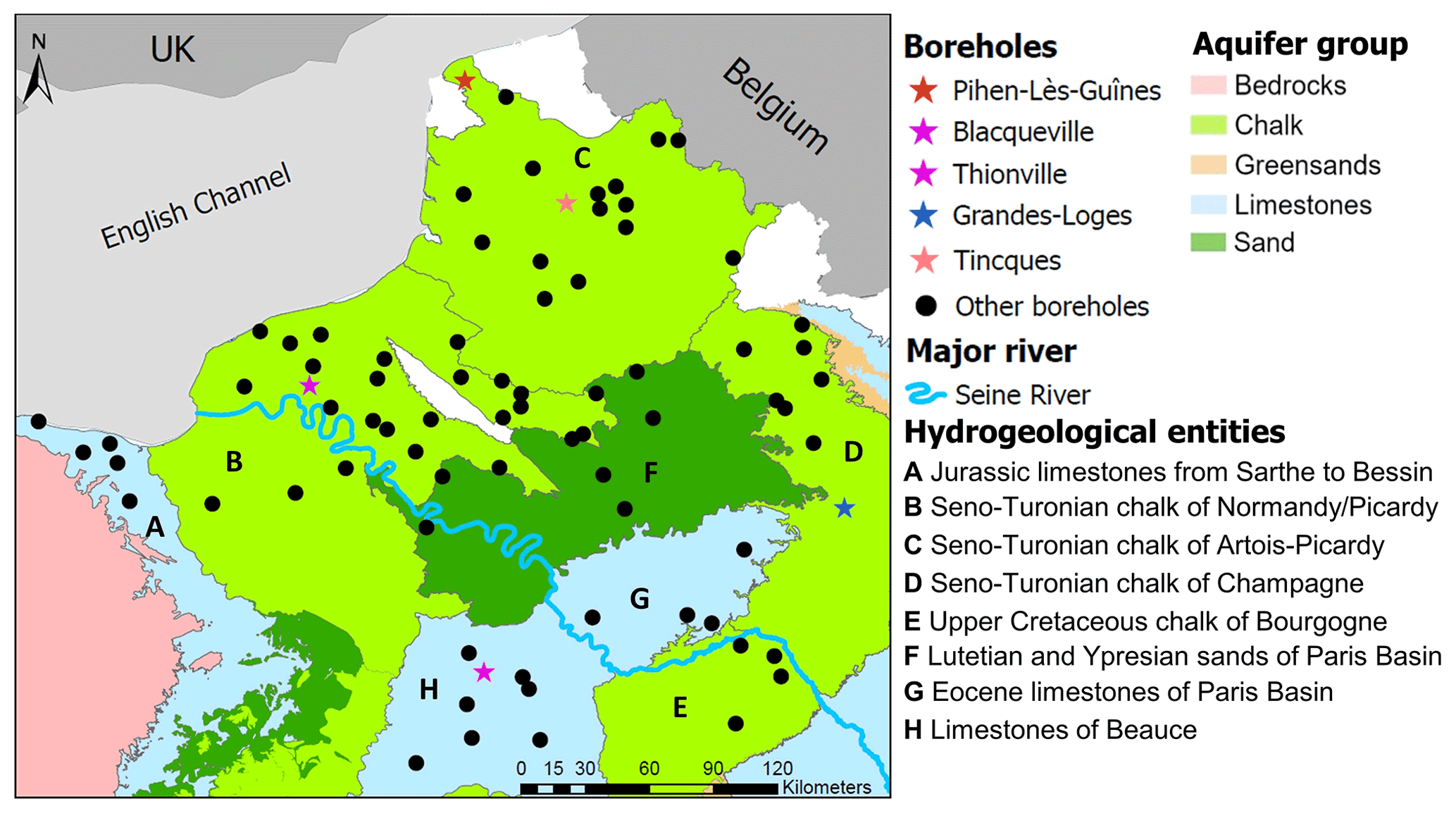
Figure 1 Spatial distribution of the 78 selected boreholes through major hydrogeological entities of the Paris Basin.

To answer this question, a simple approach based on the decomposition of GWL time series of northern French aquifers into high- and low-frequency components is proposed in this study over the 1976–2019 period. Beforehand, we quantified the variance distribution across timescales for assessing the significance of low-frequency variations in GWL signals, particularly of multi-annual (∼7-year) and decadal (∼17-year) variabilities (Sect. 4). Indeed, these ∼7- and ∼17-year variabilities have been shown to be the most important (and statistically significant) low frequencies in hydroclimatic variables and groundwater levels in northern France and neighboring countries (Slimani et al., 2009; Massei et al., 2010; Rust et al., 2019; Baulon et al., 2022). Then, our methodology consists in evaluating the influence of timescales corresponding to multi-annual and decadal variabilities by filtering one or both timescale(s) from the original signal to assess how their withdrawal affects threshold exceedance. First, we propose estimating the proportion of high levels (HLs) or low levels (LLs) associated with the multi-annual or decadal variabilities and then the combination of both (Sect. 5). We also propose determining if proportions of HLs and LLs associated with LFVs are consistent with those obtained in the short term through a long groundwater time series (106 years of data available). Second, we propose determining on four well-known historical events the contribution of multi-annual and decadal variabilities in the amplitude of threshold exceedance (ATE) and identify what parameters may control this contribution (Sect. 6). In other words, we estimate the percentage contribution of each low-frequency component to the emergence of the historical event.

2 Effective precipitation and groundwater data

For this study, we used 78 boreholes in the Paris Basin (northern France), with GWL time series being little or not affected by pumping (Fig. 1). The study area was restricted to the Paris Basin in order to carry out the analysis over a relatively long period (1976–2019). Boreholes were selected from a BRGM database and were required to be undisturbed from human activities (Baulon et al., 2020). We selected the boreholes by following the three steps below:

• i.

  a selection of boreholes with time series satisfying criteria of duration, minimum amount of data per month, and maximum length of gaps;

• ii.

  the cross-referencing of preselected boreholes with other BRGM databases on known anthropogenic influences;

• iii.

  numerous visualizations of time series with the hydrogeologists responsible for piezometric networks, in order to retain only non-influenced boreholes.

Time series of boreholes in this database were initially gathered in the ADES database that contains all groundwater data (quantity and quality) across continental France (https://ades.eaufrance.fr/, last access: 1 April 2020).

The criteria satisfied for selecting GWL time series for the present study were as follows:

• The length of time series must be higher than or at least equal to 44 years.

• The minimum amount of data within a month is set to one monthly datum before the measurement automation and three data after the measurement automation.

• The length of consecutive gaps must be <3 years for time series starting after 1950 and <10 years for time series starting before 1950. This allows time series in the new database to preserve LFV in the data. Several gaps in the time series can be allowed if these criteria are respected and if the number of gaps and their lengths are small.

Before data analysis, a visual check of the GWL time series served to remove or correct erroneous data.

The analysis of the influence of LFV on HLs and LLs was conducted over the 1976–2019 period, providing the best compromise between the spatial distribution of boreholes and time series length. In this work, all time series had a monthly time step to consider all possible GWL variation types from most reactive to most inertial ones. Then, monthly missing values were filled with linear interpolation to perform spectral analyses.

GWL time series capture chalky formations, calcareous formations, and sandy formations of the Paris Basin. In addition, we also used the GWL time series of Tincques monitoring the Seno-Turonian chalk of Artois–Picardy since 1903 (Fig. 1). This time series allowed us to perform our analysis on a longer temporal perspective and compare results with those obtained on short-term time series.

Time series of four boreholes, among the 78 of the study, were used to introduce the different GWL variation types in Paris Basin aquifers: Pihen-Lès-Guînes, Blacqueville, Thionville, and Grandes-Loges (Fig. 1). These boreholes were chosen because each of them is representative of a GWL variation type.

For the aforementioned boreholes monitoring GWL of chalk aquifers (Pihen-Lès-Guînes, Blacqueville, and Grandes-Loges), we also investigated effective precipitation (EP) corresponding to these boreholes. The gridded meteorological data – precipitation (P), snow, temperature, and Penman–Monteith potential evapotranspiration (PET) – from the SAFRAN reanalysis were used as input data to compute effective precipitation. This reanalysis provides daily data on a 8×8 km² mesh covering France from 1958 to 2019 (Vidal et al., 2010). The effective precipitation ($\mathrm{EP}=P-\mathrm{PET}$) was computed using a gridded water budget model with 8 km resolution at daily time step. It relies on the water budget method proposed by Edijatno and Michel (1989). The water budget method considers that in the water cycle, the soil acts as a reservoir characterized by its water storage capacity. Edijatno and Michel (1989) introduced a quadratic law to progressively empty the soil water reserves and to distribute the positive difference between P and PET between EP and soil storage. For each aforementioned borehole, we selected the mesh from SAFRAN reanalysis grid with the effective precipitation time series with the biggest correlation with GWL. In this study, we used monthly cumulative EP time series over the 1976–2019 period.

3 Methodological approach

3.1 Characterization of groundwater multi-timescale variability

In order to determine the prominence of LFV in GWL, the maximum overlap discrete wavelet transform (MODWT) analysis was applied. This is an iterative filtering of the time series that uses a series of low-pass and high-pass filters. Consequently, one high-frequency component called “wavelet detail” and one lower-frequency component called the “approximation” or “smooth” are produced at each timescale. At the next level, the smooth is then subsequently decomposed into another wavelet detail and smooth. The original signal can be rebuilt by summing up all wavelet details and the last smooth. The original signal is then separated into a relatively small number of wavelet components from high to low frequencies, which together explain the total variability of the signal (Fig. 2). Here, we achieved a full decomposition of the time series by applying the filter bank up to a level corresponding to the log ₂(N), where N is the length of the time series. The least asymmetric (symmlet) wavelet “s20” was used in order to better capture variability at all timescales of sometimes relatively smooth groundwater level time series.

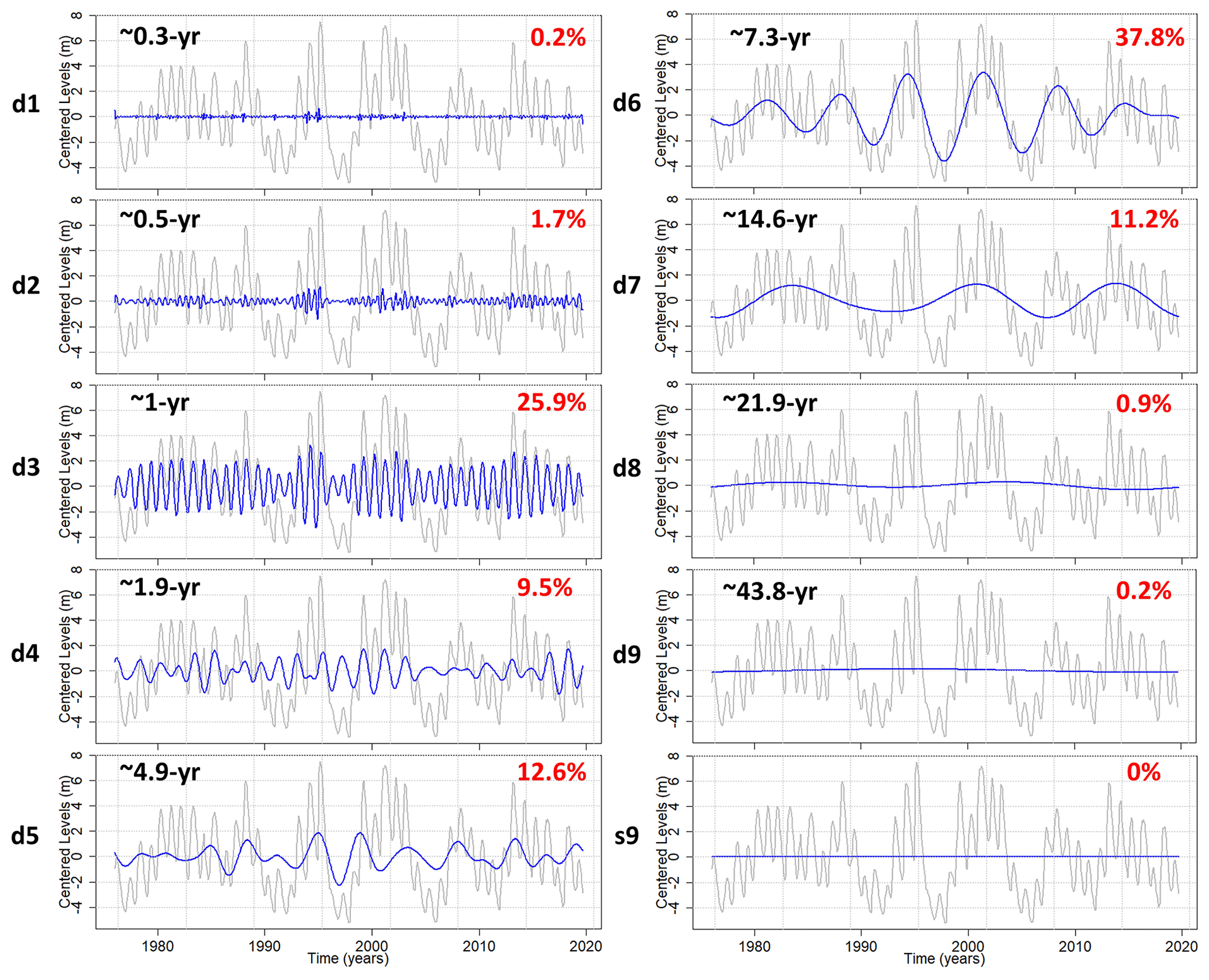
Figure 2 Example of multiresolution analysis by MODWT decomposition for the borehole of Tincques. In gray the groundwater level time series in Tincques is presented and in blue the wavelet details (d1 to d9) and the last smooth or approximation (s9). The Fourier period (in black) and energy percentage (in red) associated with each detail can be calculated.

However, unlike discrete wavelet transform (DWT), MODWT was essentially designed to prevent phase shifts in the transform coefficients at all scales by avoiding downsampling – reducing the number of coefficients by a factor of 2 – the signal with increasing scales. This results in the computed wavelet and scaling coefficients at each scale remaining aligned with the original time series; that is, the variance explained by these coefficients is located where it truly lies in the time series analyzed (Percival and Walden, 2000; Cornish et al., 2003, 2006). While not necessarily essential for signal or image processing or numerical compression, this property is fundamental for physical interpretation of the wavelet details in multiresolution analysis and has already been used for that purpose in several studies such as Percival and Mofjeld (1997), Massei et al. (2017), and Pérez Ciria et al. (2019).

The dominant frequency associated with each MODWT wavelet detail was calculated by Fourier transform of each wavelet detail (Fig. 2). The MODWT also provides the amount of variance (or energy) explained by each wavelet detail and frequency level. The energy percentage of a given wavelet detail expresses the relative importance of this variability in the total signal variability. As a result, the energy distribution between wavelet details for each borehole in the database can be extracted and mapped.

Then, we used the continuous wavelet transform (CWT) for visualizing the spectral content of GWL time series of representative boreholes of each GWL variation type in the Paris Basin. CWT is a widely used method for identifying scales of variability in environmental time series (Torrence and Compo, 1998; Labat, 2005; Liesch and Wunsch, 2019). The literature about CWT is very rich, and the theoretical background, along with an application to climatic variables, is available in Torrence and Compo (1998). The CWT produces a timescale (or time period) contour diagram on which time is indicated on the x axis, the period or scale on the y axis, and amplitude (or variance, or power) on the z axis (Fig. 3).

Figure 3 Example of CWT applied to the borehole of Pihen-Lès-Guînes. On the spectrum, time is indicated on the x axis, period or scale on the y axis, and amplitude (or variance, or power) on the z axis. The contour lines express the statistically significant regions of the spectrum at a confidence level of 95 % (Monte Carlo test). The white transparent line corresponds to the cone of influence where the variance is underestimated due to edge effects.

These analyses used R packages wmtsa (Constantine and Percival, 2016) and biwavelet (Gouhier and Grinsted, 2012).

3.2 Influence of low frequency on the occurrence of high and low groundwater levels

The influence of groundwater LFV (multi-annual and decadal) on HLs and LLs was estimated with the MODWT method for the 78 selected boreholes. As seen in Sect. 3.1, summing up all wavelet details and the last smooth rebuild the original signal. Based on this assessment, we subtracted the interest wavelet detail, corresponding to a specific timescale, from the original signal to evaluate its influence on HLs and LLs (Fig. 4a). This method allowed us to assess whether the withdrawal of multi-annual (∼7-year) and/or decadal (∼17-year) components leads to a different number and level of GWEs in the filtered groundwater time series compared to the original series.

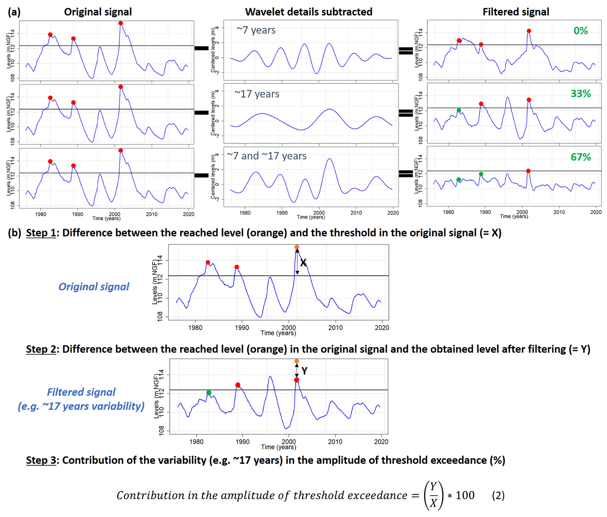
Figure 4 Workflow of (a) the influence of low-frequency variability on high and low groundwater level occurrence (example of high levels) and (b) the contribution of low-frequency variability to the amplitude of threshold exceedance. The borehole of Goupillières (chalk of Normandy) is taken as an example.

First, HLs and LLs were identified in original groundwater time series when they exceed thresholds set at the percentile 0.8 and 0.2, respectively (Fig. 4a). Percentiles 0.2 and 0.8 were determined for all boreholes of the whole dataset over the 1976–2019 period. Such percentiles were selected because they are the optimal thresholds to have a correct and sufficient number of HLs and LLs on a 44-year period, particularly for time series with inertial GWL variation type. Once these HLs or LLs have been identified, for each studied time series, details corresponding to multi-annual variability, decadal variability, and both variabilities were successively subtracted from the original signal. From these filtered time series, we evaluated if the subtraction of one given component affected HL peaks or LL peaks as initially identified in the original data. We were more particularly interested by the threshold exceedance of HL and LL peaks and their characterization as extreme levels. In the case where HL peaks still exceeded the initial threshold, the peaks remained extreme levels, so we considered that the subtracted component(s) had little influence on HL emergence. Oppositely, if peaks moved below the initial threshold, the peaks were no longer considered to be extreme levels, so we considered that the subtracted component(s) had significant influence on HL emergence since it generated the extreme level. The same assessment was realized with LL peaks.

For the sake of clarity, in this paper the terms “extremes” or “extreme levels” refer to HLs above percentile 0.8 and LLs below percentile 0.2.

For each borehole, we calculated a percentage describing the proportion of HLs or LLs in GWL generated by the considered component(s) (i.e., HLs or LLs that were no longer considered as such if the component was filtered). This calculation is presented below with HLs as an example:

$$\begin{array}{}\text{(1)}& \begin{array}{rl}& \mathrm{percentage}\mathrm{of}\mathrm{HLs}\mathrm{generated}\mathrm{by}\mathrm{the}\mathrm{component}=\\ & \left({\displaystyle \frac{\mathrm{number}\mathrm{of}\mathrm{HLs}\mathrm{moving}\mathrm{below}\mathrm{threshold}\mathrm{in}\mathrm{filtered}\mathrm{signal}}{\mathrm{number}\mathrm{of}\mathrm{HLs}\mathrm{in}\mathrm{original}\mathrm{signal}}}\right)\\ & \cdot \mathrm{100}.\end{array}\end{array}$$

Then, these results were mapped for each borehole and each filtered component (multi-annual, decadal or both).

3.3 Role of groundwater low-frequency variability in the amplitude of threshold exceedance

The calculation of the contribution of groundwater LFV in the amplitude of threshold exceedance (ATE) was achieved with the MODWT method. The methodology consisted in filtering the wavelet details of interest (corresponding to multi-annual and decadal variabilities) to estimate how they impact the amplitude of HL or LL peaks (Fig. 4b).

First, we estimated the difference between the reached level and the threshold value in the original signal (Fig. 4b; Step 1). Then, we estimated the difference between the reached level in the original signal and the obtained level after filtering the interest detail(s) (Fig. 4b; Step 2). This difference revealed the amplitude of levels carried by the subtracted detail(s). Finally, we estimated the contribution of the filtered component to the amplitude of threshold exceedance with the following equation (Fig. 4b; Step 3):

$$\begin{array}{}\text{(2)}& \mathrm{percentage}\mathrm{of}\mathrm{contribution}=\left({\displaystyle \frac{Y}{X}}\right)\cdot \mathrm{100},\end{array}$$

where Y represents the difference between the observed real level and the obtained level after filtering, and X represents the difference between the observed real level and the threshold value.

From this calculation, three types of contribution of multi-annual and/or decadal components were highlighted:

• In the case of a negative percentage, we observed an attenuation of the HL or LL peak, owing to the presence of the component considered, meaning that the level reached would have been higher (HL) or lower (LL) than actually observed without attenuation by this component.

• In the case of a positive percentage lower than 100 %, we observed an amplification of the HL or LL peak by the component, meaning that without this component the reached level was lower (HL) or higher (LL) than the actually reached level but still above (HL) or below (LL) the threshold, and the HL or LL remained an extreme.

• In case of positive percentage higher than 100 %, the HL or LL peak was generated by the component, meaning that without this component the reached level fell below (HL) or above (LL) the threshold, and the HL/LL was no longer considered as an extreme.

This analysis allowed us to better understand the contribution of the LFV in the emergence of HLs and LLs and estimate its contribution in HL/LL amplitude. It was conducted on major HL/LL events of the Paris Basin: 1995 and 2001 for HLs and 1992 and 1998 for the LLs. We focused precisely on these four events because they are currently among the most severe hydrogeological droughts and floods events across the Paris Basin (Deneux and Martin, 2001; Machard de Gramont and Mardhel, 2006; Seguin et al., 2019). Knowing that the establishment of GWL droughts may occur a few years apart between two boreholes (even in the same hydrogeological entity), we detected the LL peaks on a window extending more or less 3 years before and after the 1992 and 1998 events to be sure to correctly consider the lowest level.

4 Multi-timescale variability of groundwater levels in aquifers of the Paris Basin

Across the Paris Basin, various types of GWL variation were highlighted depending on the hydrogeological entity considered, according to the dominant timescale components which characterize their variability (Fig. 5). The Beauce limestones (entity H) are the most inertial system amongst entities of the Paris Basin with a large predominance of decadal variability (DV; purple in Fig. 5). This DV is also significant and even predominant in southern Lutetian and Ypresian sands of the Paris Basin (F) and the southern Seno-Turonian chalk of Normandy (B). Farthest north in these two hydrogeological entities, the importance of the DV shrinks to be present in almost equal proportion with the multi-annual variability (MAV; dark blue in Fig. 5). The MAV becomes predominant in the northern Seno-Turonian chalk of Normandy–Picardy (B). From eastern Seno-Turonian chalk of Normandy–Picardy (B) to northern Seno-Turonian chalk of Artois–Picardy (C), the MAV constitutes a half to a quarter of total variability, while the DV diminishes significantly in the Artois–Picardy basin.

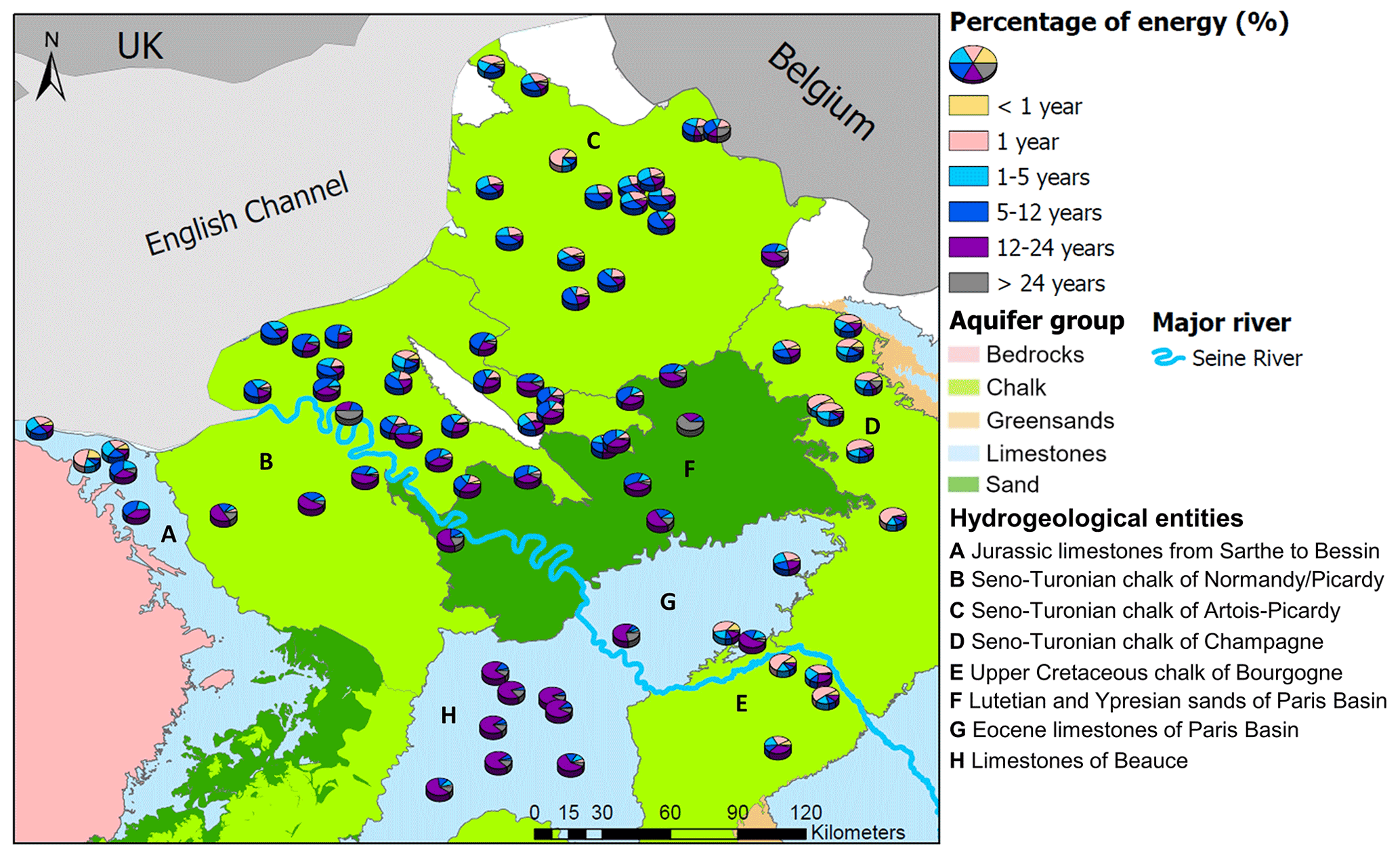
Figure 5 Multi-timescale variability of groundwater levels in the Paris Basin (78 boreholes). Pie charts describe the energy percentage of each timescale of variability reflecting their importance in total groundwater level variations. This energy percentage is derived from the MODWT analysis.

Oppositely, the annual variability (AV; pink in Fig. 5) swells from eastern Seno-Turonian chalk of Normandy–Picardy to Artois–Picardy to represent up to a quarter of total groundwater variability (Fig. 5). The AV is also significant and even predominant compared to MAV and DV in GWL of Champagne and Bourgogne chalk (D and E). These entities exhibit the most reactive water tables in our study.

Finally, the Jurassic limestones of Bessin (A) exhibit two types of GWL variation: inertial farthest south with predominant MAV and DV and more reactive on the border of English Channel, with AV and inter-annual variability (light blue in Fig. 5) accounting for a half of total variability.

No typical GWL variation was identified in the Eocene limestones of the Paris Basin (G; Fig. 5).

Overall, hydrogeological entities in the Paris Basin display four major types of GWL variation:

• type iD, inertial with a predominant decadal variability such as entity H (Figs. 5 and 6);

• type iMD, inertial with predominant multi-annual and decadal variabilities such as entities B, F and southern part of entity A (Figs. 5 and 6),

• type cAM, combined with predominant annual and multi-annual variabilities such as entity C (Figs. 5 and 6);

• type cA, combined with a predominant annual variability, such as entities D and E (Figs. 5 and 6).

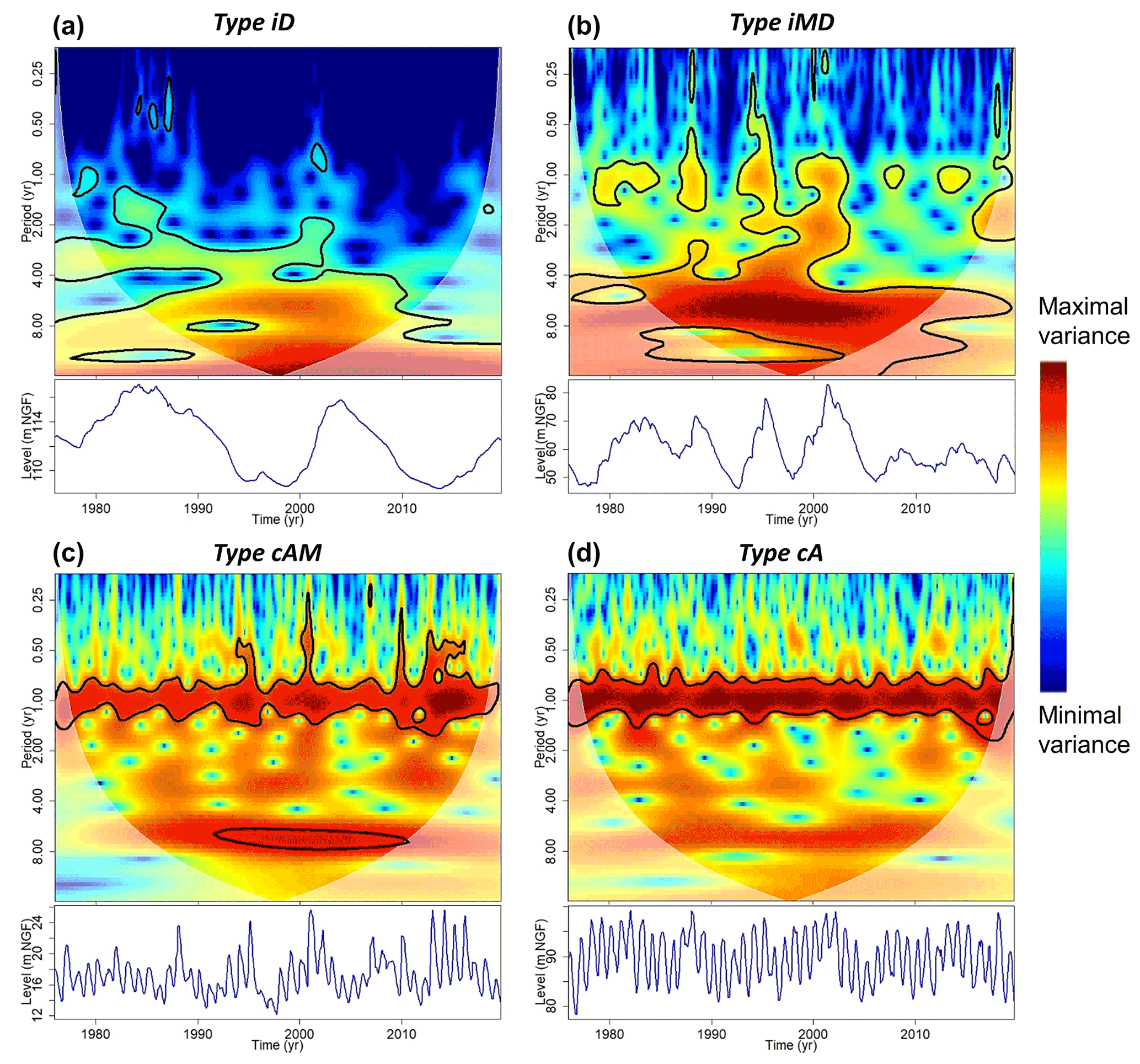
Figure 6 Time series (c, d) and wavelet spectra (a, b) of a typical time series representing each major groundwater level variation type. For type iD, this is the time series of the Thionville borehole (Beauce limestones – entity H); for type iMD, the Blacqueville borehole (chalk of Normandy – entity B); for type cAM, the Pihen-Lès-Guînes borehole (chalk of Artois–Picardy – entity C); and for type cA, the Grandes-Loges borehole (chalk of Champagne – entity D). The contour lines express the statistically significant regions of the spectrum at a confidence level of 95 % (Monte Carlo test). The white transparent line corresponds to the cone of influence where the variance is underestimated due to edge effects.

5 Influence of low-frequency variability on the occurrence of high and low groundwater levels

5.1 Spatial distribution across the Paris Basin

This section aims at determining to what extent the LFV influences the quantity of HLs and LLs in groundwater time series over the 1976–2019 period and what percentages amongst these extreme levels were generated by the MAV (∼7 years), the DV (∼17 years), and the combination of both. We specifically chose MAV and DV because they are the dominant low-frequency variabilities (and statistically significant) in groundwater levels of northern France and neighboring countries (Sect. 4; Rust et al., 2019; Baulon et al., 2022).

Figure 7 displays for each groundwater time series the number of HL peaks above a threshold set on the percentile 0.8 and LL peaks below a threshold set on the percentile 0.2 through hydrogeological entities of the Paris Basin. Type iD and iMD entities displayed the lowest number of HL and LL peaks with a decadal occurrence (H) or a multi-annual occurrence (B, F, southern A). Conversely, the quantity of HLs and LLs increased significantly in type cAM and cA entities, with a quasi-annual occurrence throughout multi-annual HLs and multi-annual LLs, respectively (entities C, D, E, and northern A). These results highlighted the significant control of the LFV on the number of HL and LL peaks: the more the LFV is predominant in GWL, the more the number of peaks is reduced because they are supported by this LFV, which naturally contains a few extremes over a relatively short period of only a few decades.

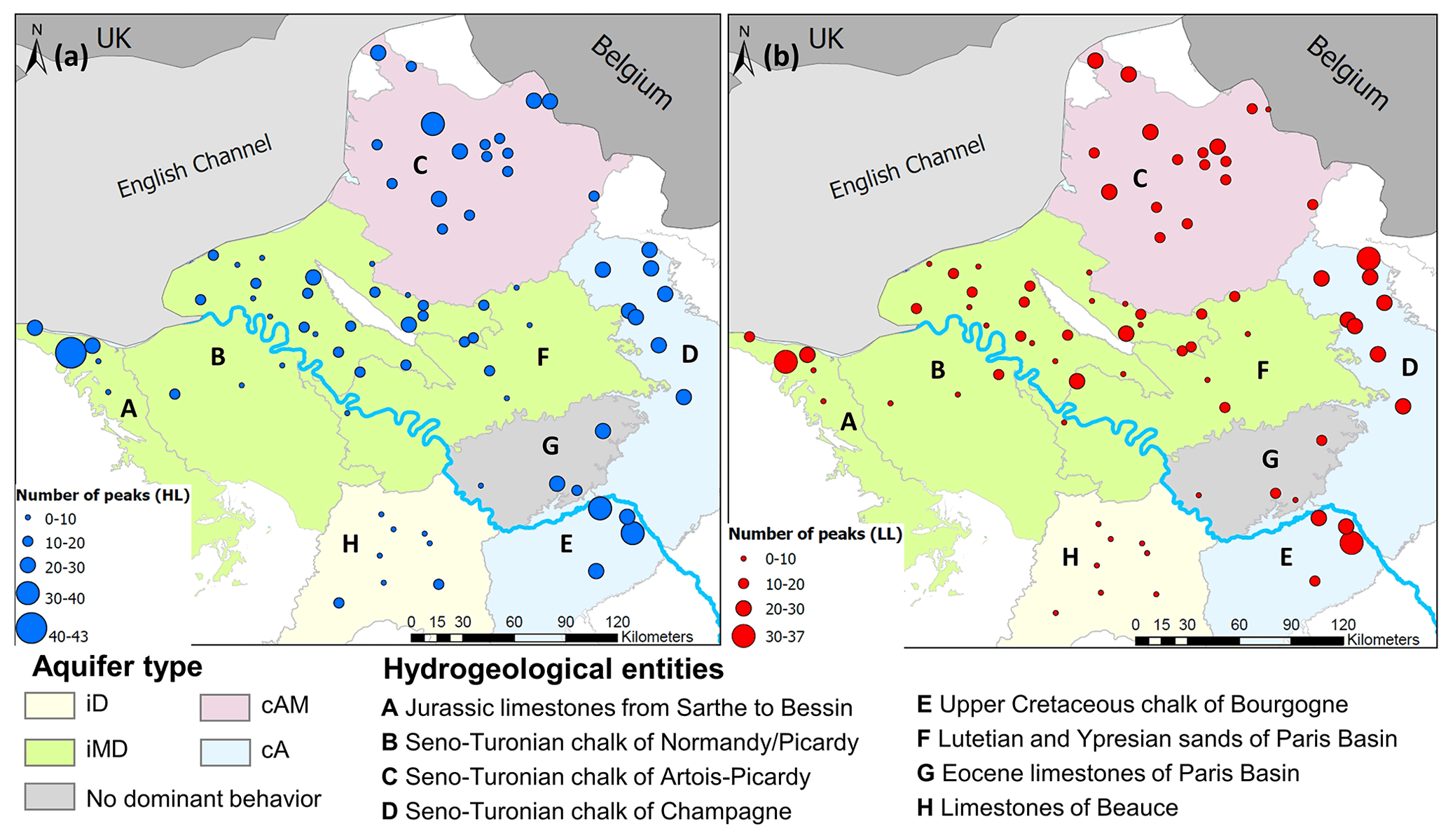
Figure 7 Number of HL peaks above percentile 0.8 (a) and LL peaks below percentile 0.2 (b) over the 1976–2019 period.

Amongst these HL and LL peaks, we estimated for each groundwater time series what percentage of HLs and LLs are generated by MAV, DV, and both variabilities (Fig. 8). The percentage of HLs and LLs generated by a given variability was closely related to the GWL variation type in hydrogeological entities.

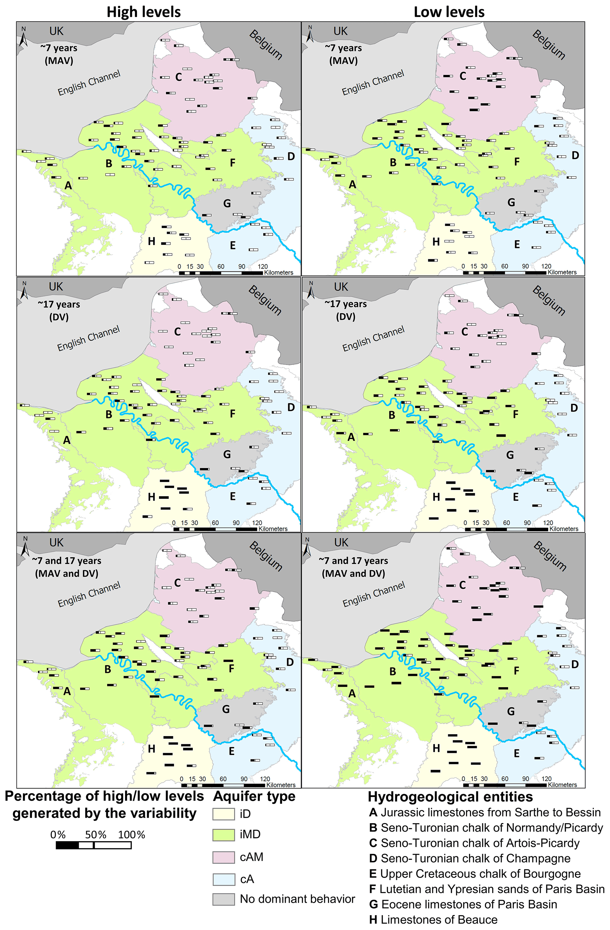
Figure 8 Percentage of HLs or LLs generated by the ∼7-year (MAV), ∼17-year (DV), and ∼7- and ∼17-year components in hydrogeological entities of the Paris Basin. This percentage corresponds to the proportion of HLs or LLs that are not considered to be extreme levels (being respectively below or above the threshold) when the component(s) is (are) absent from the original signal, meaning that these HLs or LLs are significantly supported by the component.

For the type iD entity (H), the DV generated 100 % of HLs and LLs. Exceptions were noticeable for the two southernmost boreholes that might be related to the weaker significance of the DV in GWL.

For type iMD entities (B, F, southern A), the LFV had a lesser influence on both HLs and LLs. The combination of both variabilities (MAV and DV) explained the emergence of at least 50 % of LLs. This was also often the case for HLs but in lesser proportions. Individually, the MAV and DV still explained a rather large proportion of HLs and LLs.

For the type cAM entity (C), the influence of LFVs on GWEs was reduced compared to type iD or iMD entities, particularly on HLs. A larger proportion of LLs than HLs was influenced by the LFV. Indeed, fewer than 50 % of HLs were generated by the combination of MAV and DV. Conversely, more than 50 % of LLs were generated by the combination of MAV and DV in southern C. In the northern part, the proportion approached 50 %, although it did not exceed it. This significant proportion of LLs generated by the combination of both variabilities seemed to be directly related to the influence of the MAV.

For type cA entities (D and E), the proportion of HLs and LLs generated by the LFVs was relatively small. Individually, the MAV and DV explained the emergence of less than 50 % of HLs and LLs identified in the time series. The combination of both variabilities did not allow either to explain the emergence of more than 50 % of HLs and LLs.

Overall, the LFVs seemed to have a larger influence on LLs than HLs.

5.2 One century of high and low groundwater levels and low-frequency variations

The time series used previously for assessing the spatial distribution of high and low GWL as controlled by LFV are rather short, preventing any assessment of long-term variations of high and low GWL. To explore it, the same analysis as that in Sect. 5.1. was conducted for the borehole of Tincques monitoring the Seno-Turonian chalk of Artois–Picardy (entity C) and providing data since 1903 (Figs. 9 and 10).

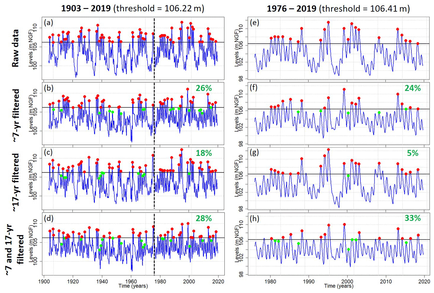
Figure 9 Influence of ∼7-year (MAV), ∼17-year (DV), and ∼7- and ∼17-year variabilities on the occurrence of HLs for the Tincques' GWL over the 1903–2019 and 1976–2019 periods. The percentage of HLs generated by the filtered component(s) (i.e., moving below the percentile 0.8) is indicated in green. The dotted black line represents the year 1976.

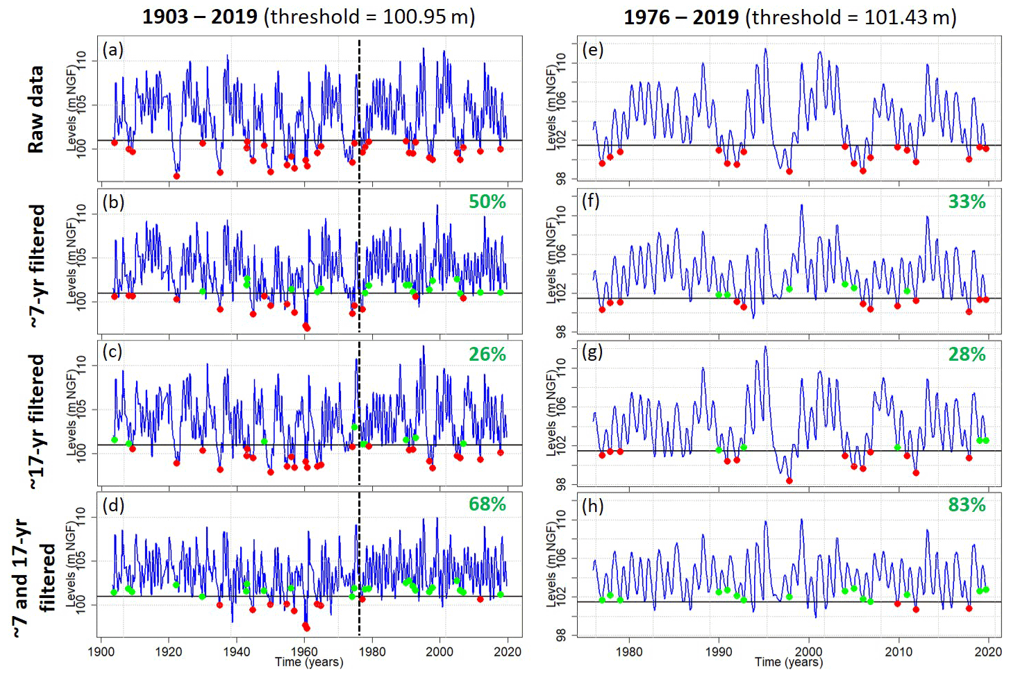
Figure 10 Influence of ∼7-year (MAV), ∼17-year (DV), and ∼7- and ∼17-year variabilities on the occurrence of LLs for the Tincques' GWL over the 1903–2019 and 1976–2019 periods. The percentage of LLs generated by the filtered component(s) (i.e., moving above the percentile 0.2) is indicated in green. The dotted black line represents the year 1976.

The predominant components of GWL variability were extracted and plotted on Fig. 11 for both 1976–2019 and 1903–2019 periods. For the long term (1903–2019), the combination of MAV and DV explained ∼50 % of GWL total variance, which is consistent with the percentage obtained for the short term for Tincques time series but also for the other GWL time series in the south part of entity C (Figs. 5 and 11).

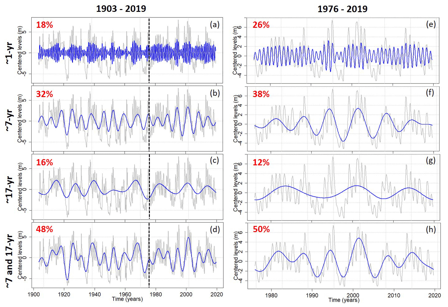
Figure 11 Maximum overlap discrete wavelet transform (MODWT) of groundwater levels at Tincques in the Seno-Turonian chalk of Artois–Picardy over the 1903–2019 and 1976–2019 periods. In gray the original time series is displayed, in blue the wavelet detail, and in red the energy percentage.

First, the identified thresholds (i.e., percentiles 0.8 and 0.2) were lower in the longer period (1903–2019) than the shorter one (1976–2019), indicating a lower GWL on average and more severe hydrogeological droughts before the 1970s (Figs. 9 and 10).

The proportions of HLs and LLs generated by the MAV, DV, and the combination of MAV and DV for both periods for Tincques (1976–2019 and 1903–2019) agreed with the ranges of percentages exhibited by boreholes monitoring the Seno-Turonian chalk of Artois–Picardy over the 1976–2019 period (Figs. 8–10). Similarly to the previous conclusions, we also observed a higher influence of LFVs on LLs than HLs (Figs. 9 and 10).

Some HLs that fell below threshold when the MAV or DV was filtered out from the original signal – and were no longer considered to be GWEs – did not fall below the threshold when both MAV and DV were filtered out, remaining GWEs (Fig. 9). For example, we can observe such a phenomenon for the third HL in the 1903–2019 period (Fig. 9b and d). This is related to the compensation between MAV and DV: the withdrawal of DV increased the level compared to raw data (Fig. 9a and c), much more than the level decreased when the MAV was filtered out (Fig. 9a and b); therefore the level stayed above the threshold when both variabilities were filtered out (Fig. 9d). The same phenomenon is visible for some LLs as well (Fig. 10).

Proportions of HLs generated by the MAV (Fig. 9b and f) or the combination of MAV and DV (Fig. 9d and h) were close between both periods (1976–2019 and 1903–2019). Over the 1903–2019 period, the HLs generated by the MAV (Fig. 9b) or the combination of MAV and DV (Fig. 9d) were regularly distributed over time. Conversely, the proportion of HLs generated by the DV was much higher for the 1903–2019 period (Fig. 9c) than the 1976–2019 period (Fig. 9g), the DV having seemingly much more influence on HLs before the 1980s.

LL peaks were found to be much more pronounced before the 1960s (Fig. 10a). The lowest level in 1921 was significantly supported by the combination of MAV and DV (Figs. 10d and 11d). The LLs between ∼1930 and ∼1970 remained present even when both MAV and DV were removed (Fig. 10d). A multidecadal LL period between ∼1930 and ∼1970, supporting the LL peaks, explained why the proportion of LLs generated by the combination of both variabilities in the 1903–2019 period (Fig. 10d) was much lower than the one displayed in the 1976–2019 period (Fig. 10h). The DV generated a similar proportion of LLs for both studied periods (Fig. 10c and g). Finally, the proportion of LLs generated by the MAV was larger over the 1903–2019 period (Fig. 10b) than the 1976–2019 period (Fig. 10f), with the majority of LLs generated by this variability emerging since the 1960s.

6 Contribution of groundwater low-frequency variability to the emergence of well-known historical events

The following subsections aim at determining the contribution of either MAV or DV or both of them to the emergence of historical events: 1995 and 2001 for HLs, 1992 and 1998 for LLs (Figs. 12 and 13). This study was based on a percentage of contribution of the ∼7-year (MAV), ∼17-year (DV), or ∼7- and ∼17-year components in the ATE. Three results can be reached: an attenuation of the HL or LL peak by the component when the percentage is <0 % (i.e., the level was higher (HL) or lower (LL) than the original level when the component was filtered), an amplification of the HL or LL peak by the component when the percentage is between 0 % and 100 % (i.e., the level was lower (HL) or higher (LL) than the original level when the component was filtered but stayed above (HL) or below (LL) the threshold and remained an extreme), and the generation of the HL or LL peak by the component when the percentage is ≥100 % (i.e., the level was no longer considered as an extreme when the component was filtered moving below (HL) or above (LL) the threshold).

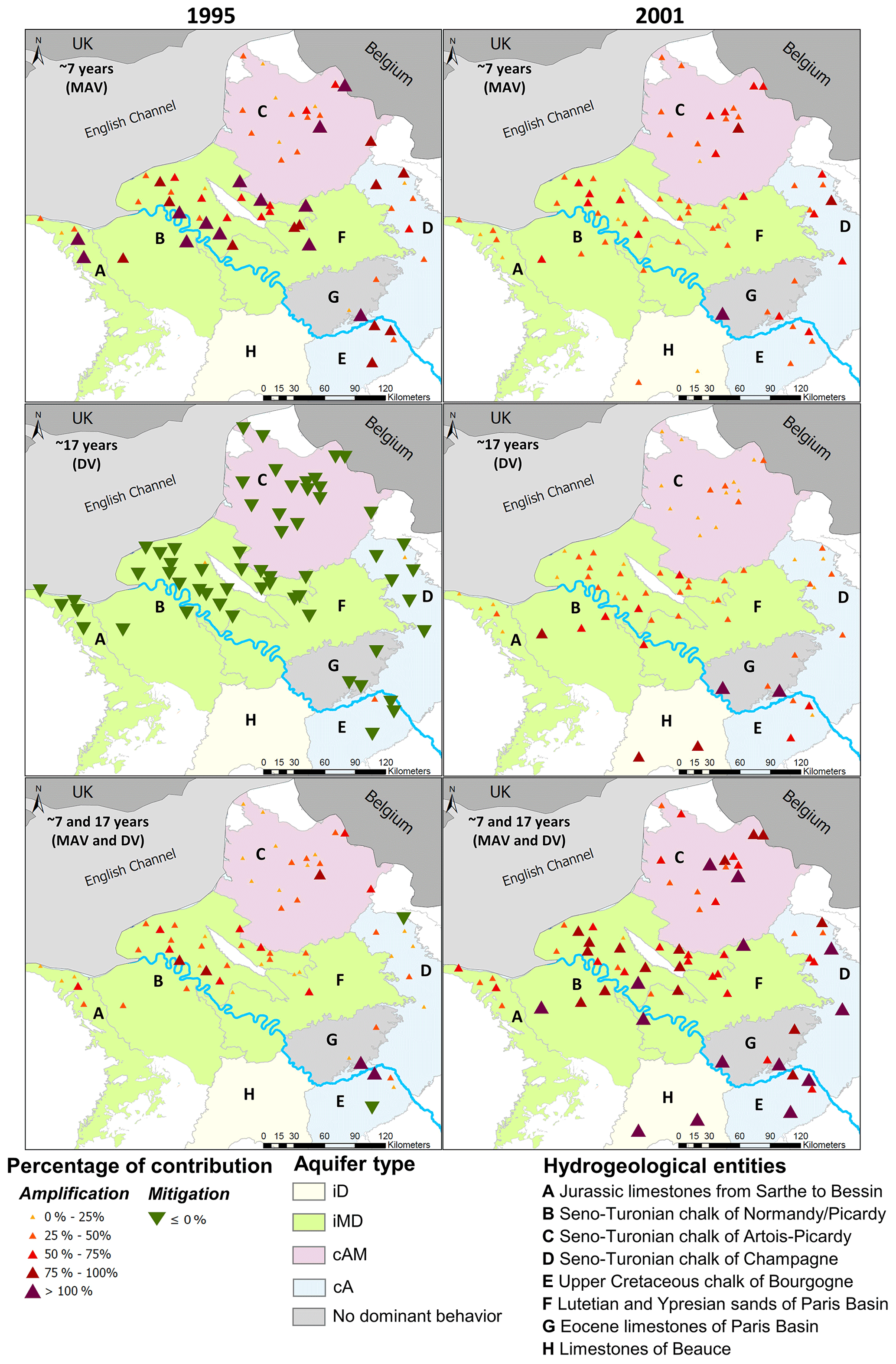
Figure 12 Contribution of ∼7-year (MAV), ∼17-year (DV), and ∼7- and ∼17-year components in the amplitude of threshold exceedance (ATE): case of 1995 and 2001 high levels (percentile 0.8). It indicates if the component generates (contribution to ATE ≥ 100 %), attenuates (contribution to ATE < 0 %), or amplifies (contribution to ATE between 0 % and 100 %) the high level. In the case of missing borehole(s) on maps, it means that either the 1995 or 2001 high level was not identified in the time series (i.e. no threshold exceedance).

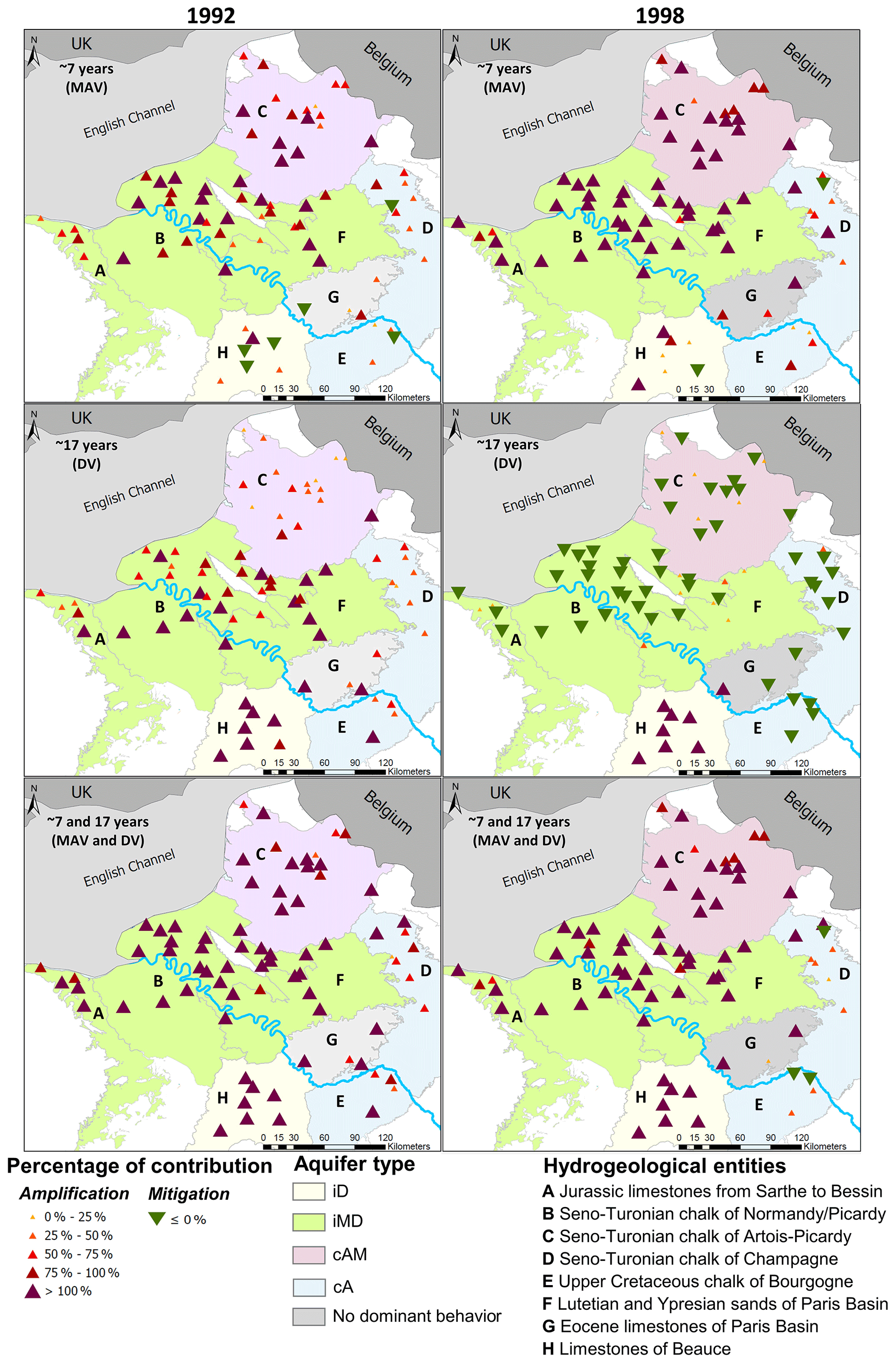
Figure 13 Contribution of ∼7-year (MAV), ∼17-year (DV), and ∼7- and ∼17-year components in the amplitude of threshold exceedance (ATE): case of 1992 and 1998 low levels (percentile 0.2). It indicates if the component generates (contribution to ATE ≥ 100 %), attenuates (contribution to ATE < 0 %), or amplifies (contribution in ATE between 0 % and 100 %) the low level. In the case of missing borehole(s) on maps, it means that either the 1992 or 1998 low level was not identified in the time series (i.e. no threshold exceedance).

In addition, Fig. 14a displays the MODWT extraction of AV (∼1-year), MAV (∼7-year), DV (∼17-year), and MAV and DV (∼7- and ∼17-year) for three boreholes representative of each GWL variation type of chalk aquifers (type iMD – Blacqueville, type cAM – Pihen-Lès-Guînes, type cA – Grandes-Loges), with the studied historical events highlighted. It provides a visual insight into the situation (i.e., positive or negative level) of these variabilities during the emergence of historical events. The same extraction is also realized in EP to be compared to GWL (Fig. 14b).

In the subsequent section, the term “concomitant situation” refers to concomitant minima or concomitant maxima levels of MAV and DV. The term “opposite situation” refers to maxima–minima or minima–maxima levels of MAV and DV.

6.1 The low-frequency origin of the selected historical events

The low-frequency origin of each historical event was spatially consistent across aquifers of the Paris Basin (Figs. 12 and 13). First, the 2001 HL and the 1992 LL resulted from a concomitant situation of MAV (∼7-year) and DV (∼17-year), both leading to the accentuation of the amplitude of the extreme level observed. Figure 14a also highlights such situations for both events via the MODWT analysis of GWL for three boreholes in the chalk. Conversely, the 1995 HL and the 1998 LL resulted from an opposite situation of the MAV and DV, leading to the attenuation of the extreme level (Figs. 12 and 13). Indeed, the 1995 HL originated from a multi-annual HL attenuated by a decadal LL, while the 1998 drought originated from a multi-annual LL attenuated by a decadal HL (Fig. 14a).

We also found such concomitant or opposite situations of MAV and DV in effective precipitation (Fig. 14b). The presence of such variabilities in EP indicates their climatic origin. Cross-correlation in Fig. 15 indicated that such LFVs in GWL lagged behind those in EP from 0 months for the most reactive system (chalk of Champagne – type cA) to 1.3 years for the most inertial system (Seno-Turonian chalk of Normandy – type iMD).

Although such concomitant or opposite situations of MAV and DV in GWL were overall consistent within and between the hydrogeological entities, some discrepancies can be highlighted locally. The influence of the DV during the 1998 drought is a typical example: while it attenuated LLs, it also sporadically amplified LLs in some places (entities A, B, C, D, F, G, and H in Fig. 13). Such discrepancies might be explained by local basin properties that may operate different filtering effects. This phenomenon was particularly recurring in the GWL of entity H, and this is developed in Sect. 6.2.1.

In addition, the contribution of each component to the ATE differed according to hydrogeological entities and the GWL variation type (Figs. 12 and 13). Therefore, the subsequent section aims at assessing the specific contribution of MAV and DV to explain the amplitude of HLs and LLs for each hydrogeological entity.

6.2 Contribution of low-frequency variabilities to amplitude of threshold exceedance

6.2.1 Type iD (inertial – decadal-dominant) hydrogeological entities

Entity H displayed the largest contribution of the LFV (i.e., the combination of MAV and DV) in the HL and LL emergence (Figs. 12 and 13). In such typical behavior with a large predominance of the DV in GWL, the LFV was involved for at least 100 % in the ATE and always generated the HL or LL, regardless of the event. This contribution is primarily related to the DV that alone is responsible for at least 75 % of the ATE. During the 1998 LL, the DV in entity H displayed an opposite influence to that of other hydrogeological entities (Fig. 13). While the DV primarily attenuated the LL peak for the other entities, it generated the LL peak in entity H. Indeed, due to its large predominance in GWL, the DV can never attenuate LL (or HL) peaks because this component supports the HL and LL peaks exclusively.

6.2.2 Type iMD (inertial – multi-annual- and decadal-dominant) hydrogeological entities

Such entities (B, F, southern A) exhibited a significant contribution of the LFV (i.e., the combination of MAV and DV) in the HL and LL emergence (Figs. 12 and 13). During the 2001 HL, the LFV was involved for at least 50 % of the ATE, and this originated from MAV and DV, which were both involved in rather similar proportions (Fig. 12). During the 1995 HL, the contribution of the LFV was more reduced due to the attenuation of the HL peak by the DV, and the threshold exceedance was related primarily to the MAV accounting for at least 50 % of the ATE (Fig. 12).

During the drought events, the contribution of the LFV was enhanced as it generated the LL events (Fig. 13). For the 1992 drought, the MAV and DV individually accounted for at least 50 % of the ATE and may even have generated the LL peak. While this event was generated primarily by the combination of a multi-annual and a decadal LL, conversely, the 1998 drought was generated by the MAV alone.

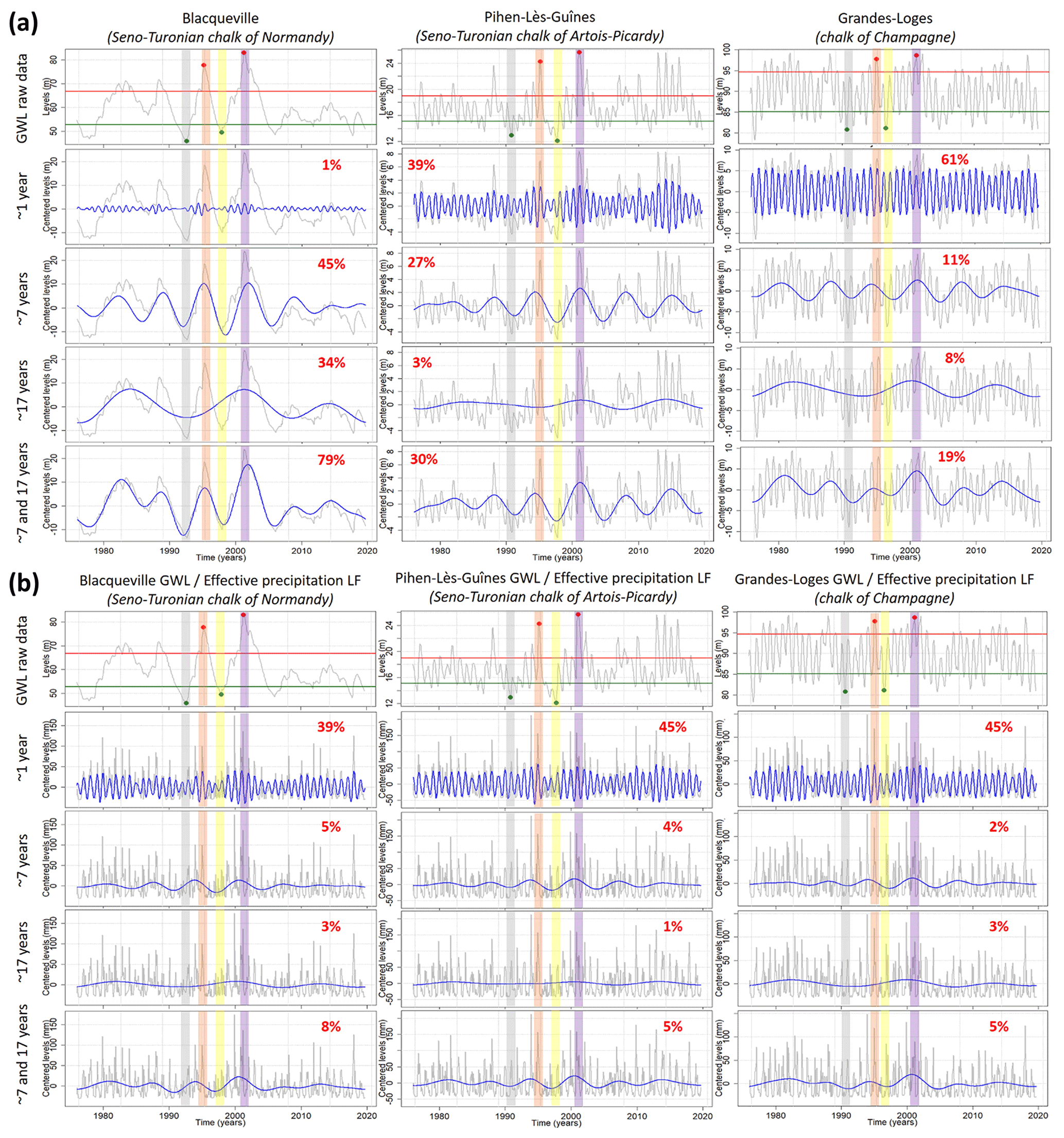
Figure 14 Extraction of ∼1-year (AV), ∼7-year (MAV), and ∼17-year (DV) components in (a) groundwater levels of three boreholes monitoring chalk aquifers and in (b) effective precipitation corresponding to the three boreholes. The 1992 low level is highlighted in gray, the 1995 high level in orange, the 1998 low level in yellow, and the 2001 high level in purple. The energy percentage of each component or association of components is indicated in red.

Figure 15 Multi-annual (∼7-year – MAV) and decadal (∼17-year – DV) components of effective precipitation (black) and groundwater levels (red) in chalk aquifers of the Paris Basin (left side). Cross-correlation between MAV and DV components of effective precipitation and groundwater levels (right side).

For the four historical events, this is primarily the MAV that drove GWL and guided a LL or a HL being reached (Fig. 14a; Blacqueville). Due to its large amplitude in GWL over the 1990–2010 period, the highest or lowest levels (over 1976–2019) were often reached during this period. Simultaneously, the DV amplified or attenuated the HL or LL that had been reached. The significance of this attenuation or amplification is directly controlled by the importance of DV in GWL but also by its phase. Hence, the greater the component accounts for a significant part in total GWL variability, the greater the attenuation or amplification. The potential dephasing and distortion of the component induced by the physical and morphometric properties of catchments may also influence the significance of the attenuation or amplification. The more the HL is at the top of decadal HL or the LL in the concavity of decadal LL, the more the amplification. And the more the LL is on the top of decadal HL or the HL in the concavity of decadal LL, the more the attenuation.

The capability of these hydrogeological entities to exhibit a significant DV in GWL, that is responsible for the amplification or the attenuation of HL and LL, caused the lowest and the highest levels (in raw data) not to be necessarily reached during the lowest and highest multi-annual levels (Fig. 14a; Blacqueville). For instance, the lowest level in the raw data was not reached in 1998 when the MAV exhibited its lowest level since the DV in positive phase attenuated this low level, but it was reached in 1992 when the low multi-annual level was less severe but accentuated by the low decadal level. Therefore in such systems, the severity of droughts and HLs depends on both MAV and DV.

6.2.3 Type cAM (combined – annual- and multi-annual-dominant) hydrogeological entities

For the entity C, the LFV (i.e., the combination of MAV and DV) was significantly involved in the LL emergence, while it was more weakly involved in the HL emergence (Figs. 12 and 13). The 1995 HL exhibited the lowest contribution of the LFV due to the opposite situation of MAV and DV (multiannual HL vs. decadal LL; Fig. 12). Consequently, LFV was involved primarily for less than 50 % in the ATE. Conversely, due to the concomitant maxima of MAV and DV during the 2001 HL, the contribution of LFV was enhanced, accounting for 25 % to 75 % of the ATE (Fig. 12). During drought events, the LFV was much more involved, accounting for at least 75 % of the ATE and may even have generated the LLs (Fig. 13).

As the DV was poorly significant in the GWL of the entity C, it was consistent that a weak contribution of this variability was observed in the emergence of the 1992 LL and the 2001 HL (Figs. 12 and 13). Conversely, the MAV was more involved because this is the predominant LFV in the GWL. In the southern C, the MAV alone generated both LL events (Fig. 13).

The weak DV in the GWL did not allow the HLs and LLs to be significantly attenuated or accentuated. In the entity C, the amplitude of a LL or HL was directly dependent on the amplitude of the MAV (without considering the AV) (Fig. 14a; Pihen-Lès-Guînes). For instance, the lowest level in raw data occurred in 1998 when the MAV exhibited its lowest level, and the 1992 LL was less severe like in the MAV. Therefore in such systems, the severity of droughts is almost only dependent on the MAV. In contrast, the severity of HLs depends on both MAV and AV.

6.2.4 Type cA (combined – annual-dominant) hydrogeological entities

Entities D and E generally displayed the slightest contribution of the LFVs in the HL and LL emergence (Figs. 12 and 13).

Generally, the contribution of the LFV (i.e., the combination of MAV and DV) to the ATE remained lower than 100 % for the four events. Locally, this contribution was higher than 100 % and generated the HL or LL. However, it remained rather rare at the scale of these two hydrogeological entities. The highest contributions of the LFV to the ATE were found during events displaying a concomitant situation of the MAV and DV (Figs. 12, 13, and 14a – Grandes-Loges). Indeed, during the 2001 HL and the 1992 LL, the LFV explained at least 50 % of the ATE. Conversely, the LFV explained less than 50 % of the ATE for events displaying an opposite situation of MAV and DV (1995 HL and 1998 LL).

Individually, the MAV was involved for less than 100 % in the ATE of these four events (Figs. 12 and 13). This contribution fluctuated significantly across the entities from 0 % to 100 % and according to the event. During the 2001 HL, the contribution of the MAV was larger than that of the DV. Conversely during the 1992 LL, the respective contribution of the MAV and DV was rather similar.

Compared to type iD, iMD, and cAM entities, differences between the contribution of the LFV to ATE during HL and LL events are less striking (Figs. 12 and 13). In addition, due to the quasi-equal energy distribution between MAV and DV (even if they remain rather weak in total variability), the severity of LLs and HLs is dependent on the amplitude of both MAV and DV (Fig. 14a; Grandes-Loges). The MAV primarily guided the emergence of a HL or a LL, while the DV accentuated or attenuated these HLs or LLs. In addition, the predominant AV can accentuate or attenuate the HL severity even more but also that of LL.

7 Discussion

The present study showed the large influence of the MAV on groundwater LL occurrence in type iMD, cAM, and cA aquifers. Simultaneously, the DV modulates the severity of droughts in aquifers for which it accounts for a significant part of GWL variability (type iMD or cA aquifers). Therefore in such contexts, the DV can significantly mitigate or amplify LL amplitude. When the DV only accounts for a small part of total variability, the severity of droughts mainly depends on the amplitude of MAV. These observations are also valid for groundwater HLs, but the influence (in proportion) of LFV on HLs is mitigated compared to LLs since the amplitude of high-frequency variabilities (intra-annual to annual variabilities) strengthens during wet periods (Fig. 14).

These LFVs, modulated in variance by catchments properties, directly result from internal climate variability (Gudmundsson et al., 2011). Numerous studies highlighted the potential link between the LFVs in hydroclimatic variables over the European continent and the LFVs of well-known climatic or oceanic modes such as the North Atlantic Oscillation (NAO) or the Atlantic Multidecadal Oscillation (AMO), also known as Atlantic Multidecadal Variability (AMV) (Massei et al., 2010; Boé and Habets, 2014; Neves et al., 2019; Liesch and Wunsch, 2019). Such links have even been very well documented and already very extensively studied for the northern France area in several studies dating back to the end of the 2000s (Massei et al., 2007, 2017; Slimani et al., 2009; El Janyani et al., 2012; Fritier et al., 2012; Massei and Fournier, 2012).

In the past, regular changes of hydrological variability (i.e., variance) have been observed at each timescale in numerous studies (Fritier et al., 2012; Dieppois et al., 2013, 2016; Massei et al., 2010, 2017; Neves et al., 2019). Knowing the dependence of GWEs on LFVs, this aperiodic behavior of LFVs can heavily influence the HL and LL severity in aquifers displaying inertial or combined GWL variation types. This is why we found varying contributions of MAV and DV in GWE emergence in our study. Indeed, there are periods where LFVs can exhibit an attenuated variance (e.g., since the end of 2000s for the ∼7-year variability; Fig. 11f) or on the contrary an accentuated variance (e.g., 1990s to 2000s for the ∼7-year variability; Fig. 11f). Hence, HLs and LLs happening during periods with an increased variance of LFV are generally much more severe than those happening during periods with attenuated variance. Therefore, this aperiodic behavior of LFVs considerably limits the predictability of groundwater droughts or more generally of GWEs.

The identification of large-scale atmospheric and oceanic states leading to variance modifications in streamflow, precipitation, and groundwater time series is still a major issue. Recently, Haslinger et al. (2021) highlighted that the increase of precipitation variability across the Alps at the interannual timescale can be related to a predominant meridional circulation (linked to a positive sea surface temperature (SST) anomaly gradient) enhancing soil moisture feedbacks, while the decrease of variability can be related to a predominant zonal circulation (linked to a negative meridional SST anomaly gradient) suppressing soil moisture feedbacks. In addition, they underlined that the increased variability of precipitation occurs during AMV positive phases at a ∼50-year timescale. Knowing the large impact of LFV amplitude changes on extreme levels, particularly on GWL due to the low-pass filter effect of aquifers, such studies should be developed to identify the drivers of variability changes for predictive purposes of extreme levels.

Although the potential link between hydrological variability and climate variability is rather well established, the long-term forecasting of large-scale variabilities (i.e., multiannual and decadal) remains complex, owing to their stochastic nature. Indeed, despite what is seemingly claimed in some studies, none of these variabilities can be considered periodic, and this is also the case of those constituting the NAO spectrum (e.g., Fernández et al., 2003) as well as the subsequent variabilities observed in hydrology. This issue constrains the robustness of climate projections, in which the internal climate variability is often poorly reproduced and appears as a major source of uncertainty (Qasmi et al., 2017). For instance, Terray and Boé (2013) estimated that uncertainties related to internal variability in precipitation projections over France in the middle of the 21st century may be as large as uncertainties due to climate models. Therefore, such uncertainties in precipitation estimation may also have a huge impact on the future estimation of aquifers' recharge and in fine on the predictability of GWL and extremes.

It must also be underlined that anthropogenic forcing may have already impacted climate variability (Lenton et al., 2008; Dong et al., 2011; Caesar et al., 2018). Moreover, Feliks et al. (2011) highlighted that interannual variabilities can be suppressed from atmospheric circulation when they are omitted from the Gulf Stream front or the SST field. Such modifications of the LFV in large-scale predictors may then influence the hydrological variability. The questions raised by such a phenomenon are as follows: to what extent could this impact the LFV in GWL and then influence extreme levels? Would that lead to more extreme levels or less extreme levels? Would that lead to more or to less severe extremes? Would this be expressed in the same way in aquifers exhibiting different GWL variation types?

The analysis of a long-term time series shows the importance of historical hindsight, particularly to highlight the influence of a multidecadal variability on GWEs. This multidecadal variability displayed by the Tincques time series when filtering MAV and DV is also highlighted in streamflow through metropolitan France (Boé and Habets, 2014; Bonnet et al., 2017, 2020). The links between this variability in streamflow and the AMV have been robustly established by Boé and Habets (2014), Bonnet et al. (2020), and previously in spring precipitation by Sutton and Dong (2012). The negative phase of multidecadal variability in streamflow and precipitation over the 1940–1960 period (corresponding to a warm period of the AMV) is also exhibited in GWL of the Artois–Picardy chalk, hindering the ATE of LLs from being fully explained by the MAV and DV (Fig. 16). Low GWLs are thus supported by a multidecadal variability, seemingly associated with the multidecadal variability in AMV. The short-term analysis could not highlight the significant contribution of multidecadal variability in GWE emergence.

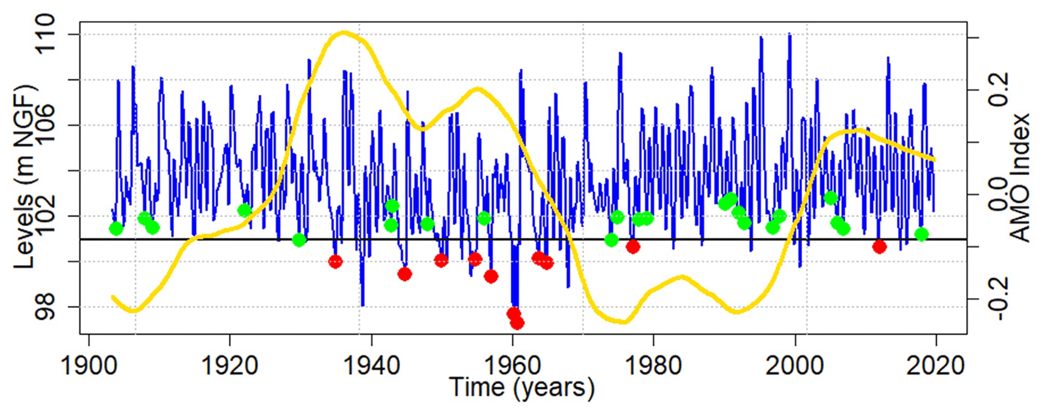
Figure 16 Same as Fig. 10 but only for the Tincques' GWL filtered of both ∼7-year (MAV) and ∼17-year (DV) components, with the Atlantic Multidecadal Variability (AMV) index superimposed in yellow. The AMV is smoothed to highlight the multidecadal variability.

The historical hindsight available for the Tincques time series also allowed us to observe tougher droughts before the 1960s, certainly related to the negative phase of the multidecadal variability (Fig. 10a). Nonetheless, the most severe drought in the Seno-Turonian chalk of Artois–Picardy appeared around 1921 (during a positive phase of the multidecadal variability). This drought was also identified as one of the most severe events across Europe in precipitation and streamflow time series (Folland et al., 2015; Caillouet et al., 2017; Rudd et al., 2017; Hanel et al., 2018; Barker et al., 2019). Bonnet et al. (2020) also identified this event as the most severe hydrological drought in the Seine River flow. However in their study, this drought did not appear as the most severe in the Beauce limestones (Toury time series), probably due to the high inertial nature of this hydrogeological entity. Indeed, in the chalk (Tincques time series), the 1921 drought seemed to be the result of the combination between a low multi-annual level and a low decadal level (Fig. 11d). The combination of both components explained the drought emergence almost exclusively. In the Beauce limestones, the MAV is poorly expressed in the GWL signal, while the larger-scale variabilities (decadal to multidecadal) are widely expressed; therefore the drought of 1921 could not have been as severe in the Beauce limestones as it was in the Seno-Turonian chalk, due to the significant role of the MAV in its emergence. Nevertheless, the positive phase of the multidecadal variability probably mitigated the severity of this drought in both aquifers.

The above example shows that a severe hydrogeological event in a given aquifer, supported by specific low-frequency variabilities, may not be as severe in another aquifer when these variabilities are not or poorly significant in total GWL variability. It highlights the resistance of aquifers to drought events for which the low-frequency components that support them do not constitute a significant part of GWL variability.

Since these hydrogeological extremes are supported primarily by the LFVs in aquifers with inertial or combined GWL variation types, and considering the large impact that they can induce on our societies (e.g., water exploitation, groundwater–river exchanges, and floods), it is fundamental to consider the LFV in GWE prediction. On the short-term horizon (i.e., annual scale), the current LFV state may help to get an idea of the emergence of a groundwater drought or flood in the near future for each type of aquifer.

• For type iD aquifers, with a downward (upward) phase of DV in GWL, the probability of heading for a groundwater drought (flood) in the short term is higher.

• For type iMD aquifers, with a concomitant downward (upward) phase of MAV and DV in the GWL, the probability of heading for a groundwater drought (flood) in the short term is higher.

• For type cAM aquifers, with a downward (upward) phase of MAV in GWL, the probability of heading for a groundwater drought (flood) is higher. However, the probability of heading for a drought or flood in the short term is also highly dependent on the AV state and the last winter recharge.

• For type cA aquifers, the same conclusions can be reached than iMD aquifers; however the probability of heading for a drought or flood in the short term also highly depends on the AV state.

However, assessing the current LFV state requires adopting the right methodology, particularly if MODWT analysis is used. The resulting low-frequency components are particularly subject to edge effects. The last values of low-frequency components are then susceptible to being biased. Consequently, it requires sufficiently long time series to extract components that are not subject to edge effects and that enable ∼7- and ∼17-year components to be distinguished from the last approximation.

On mid- and long-term horizons (i.e., several years or longer), it is necessary to identify the large-scale predictors of such variabilities for extreme level prediction purposes. In the literature, it has been demonstrated that large-scale patterns leading to the different LFVs (i.e., multiannual and decadal) may vary across timescales (Massei et al., 2017; Sidibe et al., 2019). Such an approach should also be conducted for the GWL. In addition, the response of GWEs to scenarios of changing climate variability (i.e., variance changes of LFVs) should also be investigated.

8 Conclusion

This study highlighted the heavy influence of the low-frequency variabilities (LFVs) on the occurrence of high and low groundwater levels (GWLs). First, we estimated the proportion of high levels (HLs) and low levels (LLs) among the total number of their respective occurrences that were generated by LFVs (typically multi-annual and decadal variabilities) in Paris Basin aquifers. These proportions were highly dependent on GWL variation types: for aquifers of type iD (inertial – decadal-dominant) and iMD (inertial – multi-annual- and decadal-dominant), occurrences of HLs and LLs were logically strongly influenced by LFV, conversely to type cA (combined – annual-dominant) and cAM (combined – annual- and multi-annual-dominant) aquifers. In addition, the multidecadal variability also seemed to influence occurrences of HLs and LLs, but it was only discernable on a 100-year GWL time series.

Second, we determined the contribution of the LFVs to the amplitude of threshold exceedance (ATE) during four historical events. Results highlighted that the contribution of the LFV was rather dependent on the significance of multi-annual and decadal variabilities in the total GWL variability. This contribution varied according to the event. Generally, we also observed a more significant contribution of the LFV in the ATE during LLs compared to HLs. This is related to the higher contribution of high-frequency variability (intra-annual to annual) in HL events, since its variance increases during wet periods, thus reducing the relative contribution of the LFV to the ATE of HLs.

This study also highlighted that the occurrence of a HL or LL and its amplitude (or severity) seemed primarily guided by the multi-annual variability in type iMD, cAM, and cA aquifers. The HL or LL severity can then be significantly accentuated (e.g., 2001 HL, 1992 LL) or attenuated (e.g., 1995 HL, 1998 LL) by the decadal variability.

This study presented evidence about the key role of LFV in the occurrence of HLs and LLs. Since LFV originates from large-scale stochastic climate variability as demonstrated in many previous studies in the Paris Basin or nearby regions, our results point out that (i) poor representation of LFV in general circulation model (GCM) outputs used afterwards for developing hydrological projections can result in strong uncertainty in the assessment of future hydrogeological extremes, and (ii) potential changes in the amplitude of LFV, be they natural or induced by global climate change, may lead to substantial changes in the occurrence and severity of hydrogeological extremes for the next decades. In addition, such a stochastic nature of LFV does not enable any deterministic prediction for future hydrogeological extremes on mid- and long-term horizons (i.e., several years or longer). For mid- and long-term hydrogeological extreme prediction purposes, identifying large-scale ocean–atmosphere drivers leading to such variabilities in GWL remains fundamental. Finally, future research should investigate to what extent potential changes in the amplitude of internal climate modes driving LFV could impact hydrogeological extremes.