the Creative Commons Attribution 4.0 License.
the Creative Commons Attribution 4.0 License.
 | 02 Jun 2022
Technical note: Efficient imaging of hydrological units below lakes and fjords with a floating, transient electromagnetic (FloaTEM) system
Pradip Kumar Maurya
Frederik Ersted Christensen
Masson Andy Kass
Jesper B. Pedersen
Rasmus R. Frederiksen
Nikolaj Foged
Anders Vest Christiansen
Esben Auken
Imaging geological layers beneath lakes, rivers, and shallow seawater provides detailed information critical for hydrological modeling, geologic studies, contaminant mapping, and more. However, significant engineering and interpretation challenges have limited the applications, preventing widespread adoption in aquatic environments. We have developed a towed transient electromagnetic (tTEM) system for a new, easily configurable floating, transient electromagnetic instrument (FloaTEM) capable of imaging the subsurface beneath both freshwater and saltwater. Based on the terrestrial tTEM instrument, the FloaTEM system utilizes a similar philosophy of a lightweight towed transmitter with a trailing offset receiver pulled by a small boat. The FloaTEM system is tailored to the specific freshwater or saltwater application as necessary, allowing investigations down to 100 m in freshwater environments and up to 20 m on saline waters. Through synthetic analysis, we show how the depth of investigation of the FloaTEM system greatly depends on the resistivity and thickness of the water column. The system has been successfully deployed in Denmark for a variety of hydrologic investigations, improving the ability to understand and model processes beneath water bodies. We present two freshwater applications and a saltwater application. Imaging results reveal significant heterogeneities in the sediment types below the freshwater lakes. The saline water example demonstrates that the system is capable of identifying and distinguishing clay and sand layers below the saline water column.
- Article
(9821 KB) - Full-text XML
- BibTeX
- EndNote


Understanding interactions between surface water and groundwater is necessary for effective management of water resources as they are both part of an interconnected hydrologic system (Sophocleous, 2002; Winter et al., 1998; Harvey and Gooseff, 2015). This requires knowledge of hydrogeological settings below the water column of lakes, streams, and other water bodies, in addition to properties underlying adjacent onshore areas. Non-invasive geophysical methods provide spatial information on these subsurface properties and processes across many environments; over the last few decades the methods have played a vital role in near-surface investigations (Hatch et al., 2010; Day-Lewis et al., 2006). However, deployment of surface-based geophysical investigations (as opposed to airborne systems) on water bodies has historically been difficult (Sheets and Dumouchelle, 2009; Briggs et al., 2019; Parsekian et al., 2015) while not insurmountable; this has limited the application range to some degree.

Figure 1Picture and schematic of the freshwater FloaTEM configuration, with boat, transmitter coil (TX coil), and receiver coil (RX coil). In contrast, the saltwater configuration uses a 4 m × 4 m transmitter coil.
Electrical and electromagnetic (EM) methods are the two most extensively used geophysical exploration and characterization techniques for hydrologic applications (Binley and Kemna, 2005; Danielsen et al., 2003; Christiansen et al., 2006; Auken et al., 2003; Minsley et al., 2021; Siemon et al., 2009). While classically used on land, several studies have shown that these methods can also be used on lakes, streams, or rivers. Among the electrical methods, electrical resistivity tomography (ERT) has been a common and robust technique, with applications for aquatic environments including mapping the distribution of clay sediments, mapping freshwater saturation in saltwater bay sediments (Manheim et al., 2004), estimating sediment thicknesses, and locating faults (Kwon et al., 2005). These studies deployed relatively long floating cable layouts, or streamers, of approximately 100 m, towed by a boat for collecting continuous resistivity data. Longer cable layouts, giving deeper information, limit the operational efficiency significantly. This implies that these instruments inherently have a limited depth of investigation (DOI).
Applications of transient electromagnetic (TEM) and frequency domain EM tools are reported in previous studies, e.g., discharge of groundwater to lakes and brines (Ong et al., 2010; Briggs et al., 2019) and extraction of lithium from large-scale natural brine systems (Munk et al., 2016). Airborne techniques have proved capable of mapping beneath lakes, rivers, and near-shore seas (Fitterman and Deszcz-Pan, 1998; Dickey, 2018; Rey et al., 2019), but they are costly and provide lower vertical and lateral resolution than their ground-based counterparts (Hatch et al., 2010).
There has been a growing interest in the development of a towed, waterborne EM system, as such an instrument provides continuous information with high lateral resolution. Mollidor et al. (2013) have shown an application of a commercial in-loop transient EM (TEM) system on a volcanic lake to map sediment thickness. Since the system had a large transmitter loop (18×18 m2), they encountered non-1D effects requiring 3D modeling for proper interpretation. Hatch et al. (2010) presented results from a waterborne survey where they used a floating setup of a commercial TEM system, which was used over a 40 km section of the Murray River, Australia, to monitor the influx of saline water. Micallef et al. (2020) and Gustafson et al. (2019) used control source electromagnetic systems for hydrogeologic applications in shallow seawater. These studies and systems, while effective, have limitations preventing their widespread use in waterborne applications, specifically in terms of limited DOI and horizontal resolution. An ideal system would be compact and lightweight, have a small footprint, and provide sufficient transmitter power to investigate the hydrogeological properties beneath the water column.
Recent advancements in electronics of EM instrumentation led Auken et al. (2018) to develop a ground-based towed transient electromagnetic (tTEM) system for efficient and high-resolution 3D mapping of the subsurface (Maurya et al., 2020). The tTEM system provides the necessary framework for creating a floating, towed EM system. The tTEM system is relatively compact, with the entire system extending no more than 16 m behind the towing vehicle and a maximum width of 4 m. It has high lateral resolution down to 10 m × 10 m. The tTEM also has a relatively high transmitter moment for such a compact system, providing depths of investigation in ground-based surveys down to 100 m. The waterborne version of the tTEM system is referred to as FloaTEM (see Fig. 1), and a recent application of the FloaTEM system has been presented by Lane et al. (2020) where they successfully used the ground configuration of the system on rivers and estuaries in the United States to characterize the underlying hydrological system. In their study the system was used as it was designed for ground-based applications (Auken et al., 2018) without any modifications to actual geometry and measurement protocols. In this paper, we present a greatly improved and flexible version of the FloaTEM system to investigate subsurface properties beneath both fresh and saline water columns. We highlight the design aspects of the system and discuss capabilities and limitations. Finally, we present three case studies to demonstrate the efficacy of the FloaTEM system and interpretation methodology: surveying on a shallow freshwater lake, a deep freshwater lake, and in a saline bay environment.
Operating in aquatic environments provides challenges that are unique to the setting, requiring modifications not only to the instrumentation relative to land-based operation but also to acquisition protocols and safety procedures. Navigating on shallow water, lakes, or rivers may be challenging; to assist safe navigation, real-time GPS and echo-sounder data are integrated into the FloaTEM system's recording and navigation software. The echo sounder provides the depth to the riverbed or lake bed, and this information can furthermore be utilized as prior information in later data processing.
Design aspects of the FloaTEM system depend on the application – primarily whether freshwater or saltwater; thus, we have designed both a freshwater FloaTEM system (FW-FloaTEM) and a saltwater FloaTEM system (SW-FloaTEM). In the following subsections, we discuss the details of freshwater and saltwater FloaTEM systems.
2.1 The freshwater FloaTEM system
The FW-FloaTEM has a design similar to the tTEM system: a 4×2 m2 single-turn transmitter coil (TX coil) is followed by the receiver coil (RX coil) in a 9 m offset configuration. Figure 1 shows a schematic layout and photo of the FW-FloaTEM system. The receiver coil has an effective area of 20 m2 with a bandwidth of 420 kHz. This effective RX area is 4 times higher compared to the previously used RX coil of the tTEM system as described in Auken et al. (2018), and it therefore provides an approximately 4 times better signal-to-noise ratio and increased DOI (100 m).
The fiberglass frame follows the same construction as the tTEM system – mounted on two paddleboards instead of sleds – and with additional frame components added for stability. The RX coil is simply mounted on an inflatable rubber boat. Note that all mounting and floatation devices of the TX coil and RX coil are of non-conductive materials to avoid EM bias signals in the data.
The acquisition protocol consists of an alternating high- and low-moment transmitter pulse to obtain the sounding curve. The low moment, with a peak current of ∼3 A, records 15 time gates of data between 4 and 33 µs referenced to the beginning of the turn-off time of the transmitter pulse. The high-moment pulse utilizes 23 gates from 10 to 900 µs with a peak current of ∼30 A. Thanks to the latest hardware modification, the peak current is maintained with a deviation of ±0.1 A, which ensures a stable current waveform throughout the operation. Detailed system parameters are listed in Table 1.
Table 1System parameters for the freshwater and saltwater FloaTEM systems.

2.2 The saltwater FloaTEM system
Presence of highly conductive saltwater limits the DOI due to the slow diffusion of the eddy currents in the conductive water body. In order to increase the DOI, the transmitter moment of the SW-FloaTEM is increased by a factor of 8, compared to FW-FloaTEM, by doubling the transmitter loop size and increasing the number of TX coil turns to four. The saltwater configuration only utilizes a high-moment (HM) pulse of 25 A, which is sufficient to obtain a similar near-surface resolution as the freshwater system since the long-duration eddy currents in conductive seawater obviate the need to record very early times. Further justification for using only HM is given in Sect. 3. Table 1 shows the parameters for FW-FloaTEM and SW-FloaTEM systems. Observe that the last measurement gate for SW-FloaTEM is ∼3 ms compared to ∼1 ms for FW-FloaTEM system.
The signal-to-noise ratio () is further increased by using a 40 m2 RX coil. As the limiting factor for these RX coils is the noise in the preamplifier (Nyboe and Sørensen, 2012), increasing the area of the coil increases the ratio proportionally. This is true as long as the area is below approximately 200 m2. Hence, the total ratio increase for the SW-FloaTEM system compared to the FW-FloaTEM system is a factor of 8 for the peak moment and a factor of 2 for the RX coil, which is in total a factor of 16.
A model resolution study was conducted to investigate the influence of water depth and water conductivity on the resolving capabilities of FloaTEM systems for the underwater layers. The focus of the resolution study was the case of a saltwater environment, where the conductive water layer limits the DOI significantly and decreases the resolution of underwater resistivity structures. Conclusions derived from the model resolution study lead to the design of the SW-FloaTEM system. We also present the analyses of the FW-FloaTEM system to compare against the SW-FloaTEM system. The model resolution study comprises (a) an inversion of synthetically generated data from known layered models (the true model), (b) a model parameter analysis of the true models, and (c) an estimated depth of investigation (DOI). The modeling was performed with a 1D framework and hence does not examine lateral resolution capabilities or ability to resolve 2D or 3D structures.
The modeling scheme consists of the following steps:
-
calculate system-specific 1D forward data of the true model,
-
estimate realistic data uncertainties on the forward data based on signal levels and background noise assumptions,
-
estimate model parameter uncertainties by a computation of the model covariance matrix for the true model (Auken et al., 2015), and
-
perform 1D smooth inversions of the forward data including DOI estimates (Christiansen Vest and Auken, 2012).
All the modeling studies were carried out with the AarhusInv modeling code (Auken et al., 2015). The FW-FloaTEM and SW-FloaTEM systems were modeled as described in Table 1. The data uncertainty was model dependent, based on a background noise level at 1 nV m−2 at 1 ms plus a uniform contribution of 3 %. The uniform uncertainty is the main contribution to data uncertainty due to the relatively conductive models producing high signals. For the model parameter analysis, a priori constraints on the water column were applied with a 10 % uncertainty for the water depth and a 30 % uncertainty for the resistivity of the water. For the inversion, no lateral constraints were applied. However, for the model parameter analysis lateral constraints were assumed between five similar neighboring models (based on the true model) to simulate the improved resolution capabilities from information sharing when working with field data. For the inversion of the forward data, a smooth 30-layer model description was used with logarithmic increasing layer thicknesses with depth and with an additional top layer representing the depth and resistivity of the water column. All inversions were carried out using a homogeneous starting resistivity model.
Two model sweeps were constructed, each consisting of 15 three-layer models (true models). In model sweep 1 (Fig. 2a), the thickness (water depth) of a 0.3 Ωm top layer was varied from 1 to 15 m. In model sweep 2 (Fig. 3a), the resistivity of a 7 m thick water layer was varied from 0.1–3 Ωm. In both model sweeps, the second layer was 3 Ωm (10 m thick) and the third layer was 30 Ωm.
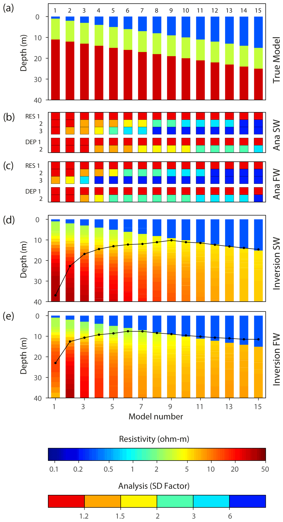
Figure 2(a) True model. The number on top of each model bar states the water depth (thickness of first layer). (b, c) Model parameter analyses of the true models, stated as a standard deviation factor, for the SW-FloaTEM and FW-FloaTEM systems. (d, e) Inversion results for SW-FloaTEM and FW-FloaTEM systems. The black line shows the DOI.
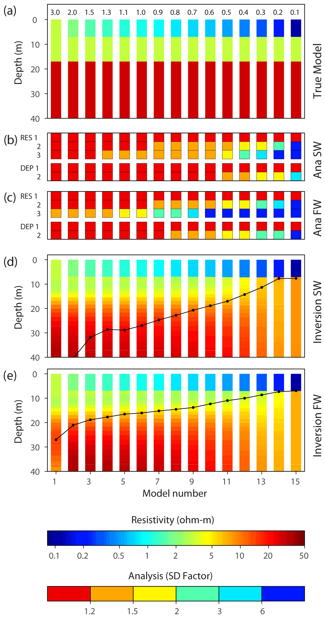
Figure 3Model sweep 2. (a) True model. The number on top of each model bar states the resistivity of the water (resistivity of first layer). (b, c) Model parameter analysis of the true model, stated as standard deviation factor, for the SW-FloaTEM and FW-FloaTEM systems. (d, e) Inversion results for SW-FloaTEM and FW-FloaTEM systems. The black line shows the DOI.
The modeling results for model sweep 1 are shown in Fig. 2. Since the modeling was carried out in log-model space, the model parameter analysis (Fig. 2b and c) shows the relative uncertainty estimates (SD factor) of the model parameters. In general, a model parameter (resistivity or thickness) will be considered resolved if the SD factor is less than 1.5, moderately resolved if between 1.5–2.0, and unresolved if greater than 2. From the model parameter analysis in Fig. 2b and c, we observe, as expected, that the resolution of the model in general decreases with increasing water depth. The water layer is very well resolved in all cases partly because of the prior constraints and partly due to the method's high sensitivity to the conductive water layer. In the SW-FloaTEM case (Fig. 2b), the resistivity of the second layer is resolved (SD factor < 2) to a water depth of about 7 m, and the layer boundary between layer two and three (DEP2) is resolved to a water depth of about 10 m. In the FW-FloaTEM case (Fig. 2c), the resistivity of the second layer is resolved (SD factor < 2) to a water depth of about 5 m, and the layer boundary to a water depth of only around 4 m. Also, for the third layer, the resistivity was better resolved in the SW-FloaTEM system case than in the FW case.
The inversion results of the true model data, with DOI estimates in Fig. 2d and e, are in line with the observations from the model parameter analysis. Increasing water depth results in a shallower DOI and loss of resolution of the underwater layers, and the SW-FloaTEM system performs better than the FW-FloaTEM system.
Water depth is not the only parameter of importance for the resolution capabilities; the resistivity or conductivity of the water is also important. Figure 3 shows the modeling results for model sweep 2 with a varying resistivity of a 7 m thick water layer. For a very conductive water layer of 0.1–0.2 Ωm, the resolution is limited for both systems, as observed in the model parameter analysis as well as in the inversion sections of Fig. 3. When the water resistivity is above 0.3–0.4 Ωm, the SW system resolves or recovers the underwater layers very well (Fig. 3b and d). Especially when resolving the boundary between second and third layer (DEP2), the SW system performs much better than the FW system, which is also clearly reflected in the DOI of the two systems.
Based on the presented analysis and other analyses (not shown in this paper), we conclude that the conductance (product of conductivity and thickness) of the water column should be below approximately 25 S (siemens) for this particular SW-FloaTEM system to be able to penetrate the water column and map underwater layers. It was also clear that the ratio for the SW system had to be increased significantly compared to the FW system. But the very early-time gates were not needed, and a slower turn-off time and lower bandwidth of the RX coil was acceptable. This led to the compromise of more turns in the transmitter coil, only high-moment cycles, and the larger area of the RX coil.
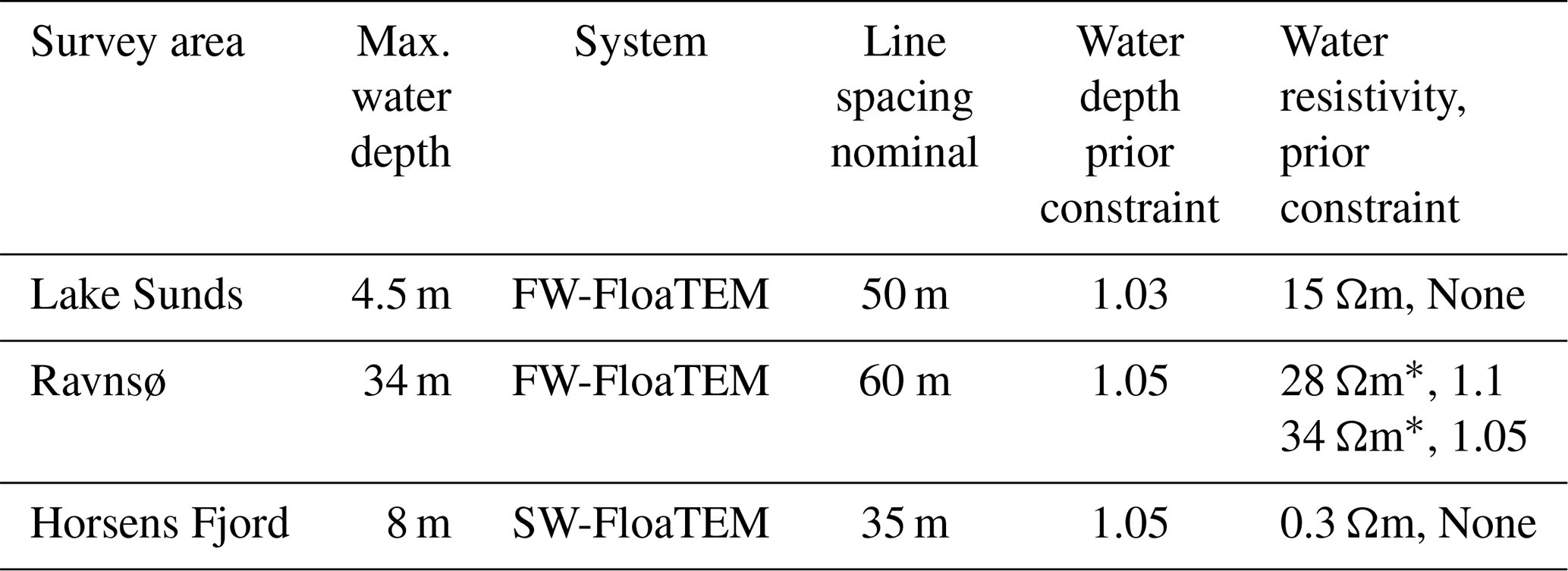
We present three surveys conducted with the FloaTEM system in Denmark: two on freshwater lakes and one on seawater in a fjord. These datasets represent different water conductivities and various glacial sediment settings. Details of processing and inversion of FloaTEM data are given in Appendix A. Some of the cases needed special handling of the inversion process, and this is described in the respective case study sections. Table 2 summarizes key survey conditions and modeling parameters.
Table 2Survey configuration and conditions of the three cases. The * indicates that the water column was modeled with two resistivity layers.
4.1 Freshwater cases
We present two freshwater cases from two lakes in central Jutland, Denmark, to demonstrate the utility of the FloaTEM-FW system in shallow- and deep-lake scenarios.
4.1.1 Lake Sunds
Lake Sunds spans 127 ha and is quite shallow (1.5–2.5 m) with a maximum depth of 4.5 m. It is sitting in a late Weichselian meltwater plain. The city of Sunds has developed around the lake, and the majority of the ∼4000 inhabitants of Sunds live close to the water. In recent years the groundwater table in Sunds has risen substantially, which causes problems in the winter period when the groundwater is the highest and periods of heavy rain then result in flooded cellars in residential houses. The problem is exacerbated by an old sewage system in the city with many worn pipes. These pipes are undergoing replacement, but this will remove the current drainage by worn pipes, and the consequences would be a further rise of the groundwater table. On top of the flooding of cellars, there is a risk that the groundwater fluctuations can mobilize near-surface pollutants from otherwise hydrologically inactive point-source pollution in the city such as old gas stations and landfills and hence contaminate the groundwater in the area.
From a hydrogeological viewpoint, the shallow water table has puzzled water managers as shallow boreholes from the area show that the geology in the upper 20 m is pure sand as expected in a meltwater plain environment. It was therefore decided to set up a detailed groundwater model to investigate groundwater flow paths and identify measures to control the groundwater table fluctuations.
The area to the east of the lake has been mapped with tTEM, covering a total of 816 ha, with a FloaTEM survey subsequently performed on the lake (Fig. 4). Additionally, multiple boreholes provide lithological data for comparison, although the majority of the boreholes only reach 10–20 m depth. Most of them were drilled in the 1940s in connection to brown-coal mapping.
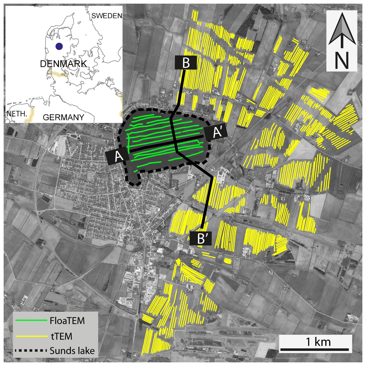
Figure 4Sunds FloaTEM and tTEM survey region with FloaTEM lines marked in green and tTEM in yellow. AA′ and BB′ are the profiles that are presented in Fig. 5.
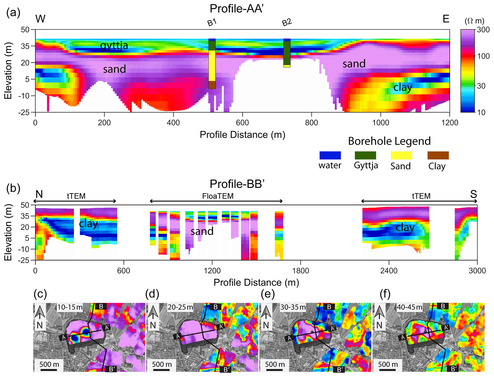
Figure 5Results from Sunds joint tTEM and FloaTEM survey. Panels (a) and (b) show the resistivity model along profiles AA′ and BB′, respectively; the locations of profiles AA′ and BB′ are marked in Fig. 4. Note that while the elevation axis is identical, the profiles have different lengths and thereby different vertical exaggeration. Profile AA′ includes lithological interpretations from available boreholes near the survey line. Note that the water column is included in the figure but only 2 m thick; panels (c)–(f) show mean resistivity maps at various depth intervals with profiles AA′ and BB′ indicated as solid black line. Lake Sunds is marked with a dotted black line.
The tTEM and FloaTEM data were inverted separately, with the results combined in Fig. 5. Profile A in Fig. 4 is entirely on the lake, and profile B is oriented north–south crossing the lake. In profile A, FloaTEM inversion results generally show a good agreement with the available borehole description (B1 and B2), which is broadly categorized as sand-, clay-, and silt-containing organic material. However, there is a slight mismatch between lithological boundaries observed in some boreholes and inversion models. This mismatch may be caused by borehole offset from FloaTEM profiles, possibly exaggerated by erroneous location data for the more than 70-year-old logs. The distances of boreholes B1 and B2 from the profile are 20 and 25 m, respectively. Overall, the resistivity model indicates a presence of two areas with a thick organic silt layer below the water column (Fig. 5a and c) followed by a thick and more resistive sand layer. The sand layer thins out towards the bank of the lake and appears to go to the surface outside the lake as indicated in profile B. The information about thickness and location of the organic silts is of great importance in the groundwater model of the area, since these old lake deposits are impermeable and thereby guide groundwater flow beneath the lake.
Figure 5c–f show mean resistivity maps at four depth intervals and include both the FloaTEM and the tTEM survey results. The mean resistivity maps indicate that there is a large degree of spatial variability of sediment types in and around Lake Sunds. The heterogeneity beneath the lake would not be possible to resolve by interpolating across; this heterogeneity is related to the lake genesis and reveals where the water table beneath the town of Sunds is in hydrologic contact with the lake. Furthermore, the tTEM and FloaTEM results show that the geological setting is not a simple sandbox at depth. At 20 m depth and below, we have several Tertiary clay layers with a resistivity of 10–30 Ωm, which have been deformed by glaciers and glacial tectonics. The information about the clay layers is crucial for the deeper parts of the groundwater model.
4.1.2 Ravnsø
Ravnsø is a lake located in eastern Jutland, Denmark. It is the second deepest lake in Denmark with depths generally ranging from 25 to 30 m and with a maximum depth of 34 m. The lake was formed as a dead-ice hole located on top of a WSW–ENE-oriented partly buried valley (Sandersen, 2016).
In the rOpen project (https://hgg.au.dk/projects/ropen-nitrate-retention, last access: 27 May 2022), the Javngyde watershed northwest of Ravnsø was mapped in detail with tTEM, and it was modeled with a 3D finite difference groundwater flow model. The purpose of the rOpen project was to estimate the total amount of nitrate reduction along flow pathways from the water table to a surface water recipient. The rOpen work and a related hydrological modeling study (Rumph Frederiksen and Molina-Navarro, 2021) revealed that around 40 % of the infiltrating water crossed the surface watershed as groundwater flow to Ravnsø. However, the hydraulic connectivity between the watershed and the lake was poorly understood, and it was decided to perform a FloaTEM survey on the lake to obtain more information about the hydrological system.
The survey was conducted with east–west-oriented lines with a spacing of 60 m combined with lines encompassing the perimeter of the lake (Fig. 6). Only electric boat engines are allowed on the lake, limiting the acquisition speed to 6 km h−1. Strong winds on the day of acquisition further challenged the navigation, resulting in headwind lines being more wiggly than the tailwind lines.
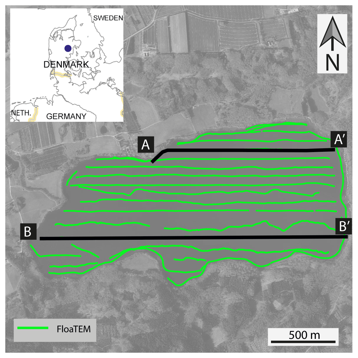
Figure 6Survey region for the Ravnsø FloaTEM survey. Locations of the profiles in Fig. 7 are highlighted as solid black lines.
The resistivity model for Ravnsø (Fig. 7) shows multiple features of interest. The relatively high resistivity of the lake water has allowed for extended depths of investigation, despite the deep-water column. The resistivity models have a DOI down to 90 m below the lake surface. Within the water column, we see resistivity changes, and this is verified by direct current resistivity measurements conducted in 0.5 m depth intervals at multiple locations (not shown). The water resistivity measurements were conducted using a 10 cm Wenner configuration. The measured resistivity of the water column gradually varies from the top to the bottom of the lake from ∼27 to ∼34 Ωm, probably due to temperature variations. For this reason, the water column was modeled with two resistivity layers with a priori constrained resistivity values and a constrained water depth (depth to bottom of second water layer) but with a free interface between the two water layers. Beneath the bottom of the lake (profiles AA′ and BB′ in Fig. 6), we observe sandy layers, underlain by a clay layer interpreted to be Oligocene. Below the bottom of the lake, we observe a thin conductive layer which is interpreted as fine sediment deposits such as clay or silt. The mean resistivity maps (Fig. 7c–f) at different depths reveal a large heterogeneity in the geology below Ravnsø. Along the shore of the lake, we observe sandy deposits, which most likely play an important role in discharging groundwater to the lake.

Figure 7Results from Ravnsø FloaTEM survey. Panels (a) and (b) show the resistivity model along profiles AA′ and BB′, respectively; the locations of profiles AA′ and BB′ are marked in Fig. 6. The black line in the sections marks the lake bottom, while the white faded colors indicate the DOI. Panels (c)–(f) show mean resistivity maps at four depth intervals below surface together with locations of profiles AA′ and BB′.
4.2 Saltwater study
Horsens bay is a shallow fjord located in the western Baltic Sea, Denmark, roughly 18 km long and 2–3 km wide. It has poor ecological status, possibly due to submarine groundwater discharge causing excessive loading of nutrients (Hinsby et al., 2012). Increased loading of nutrients has caused the Baltic Sea to be one of the most polluted seas in the world (Pihlainen et al., 2020; Meier et al., 2019). To understand the vulnerability of the Horsens Fjord and coastal zone dynamics, an improved understanding of land–sea interactions including contaminant pathways in the subsurface, in relation to nutrient and salinity variations, is needed.
The water depth within the survey area (Fig. 8) ranges from 2 m (minimum water depth for safe maneuverability with the specific vessel) to 8 m in the central area. FloaTEM data were acquired in north–south-striking lines across the bay (Fig. 8), with a line spacing of ∼25 m and an operational speed of 12–14 km h−1. The relatively small survey was conducted in collaboration with the Geological Survey of Denmark and Greenland (GEUS). The purpose was to identify and map fresh groundwater flow into the fjord, which may provide pathways for nitrate leaching from the surrounding farmland into the bay. The geology beneath Horsens Fjord includes Quaternary meltwater sand and gravel constituting as aquifer and Quaternary clay tills and Miocene mica clay as aquitards (Jørgensen et al., 2010). A narrow channel connects the fjord to deeper waters in the Baltic Sea. The central part of the fjord is dominated by muddy sediments due to the high accumulation of organic material. Till deposits are present in shallow coastal areas.
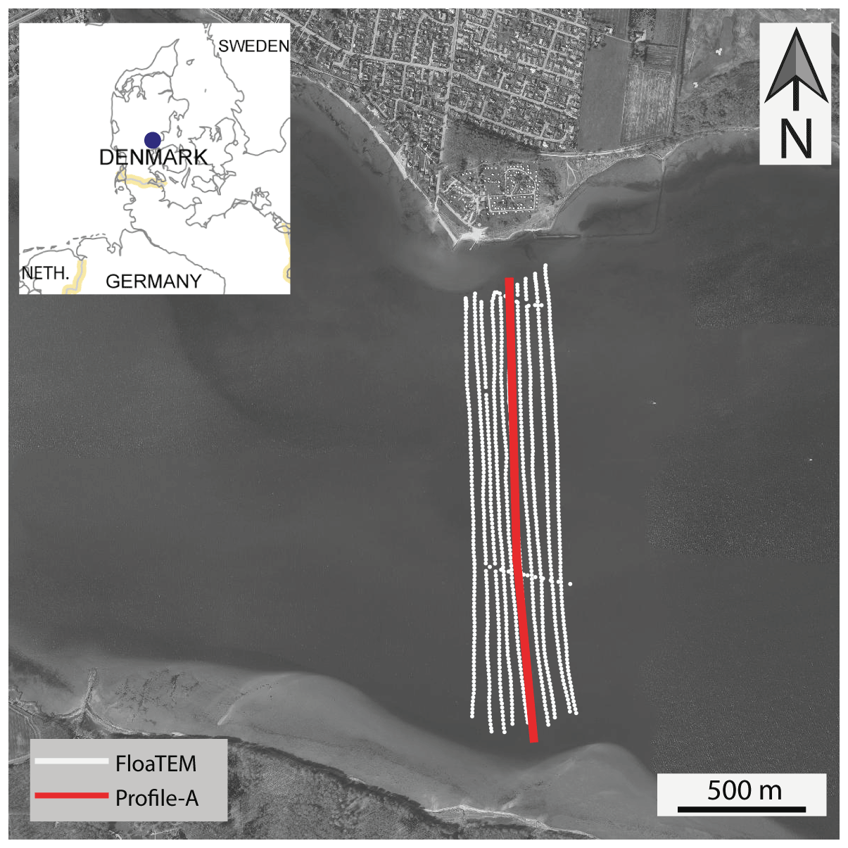
Figure 8Horsens bay with FloaTEM survey lines. The red highlighted profile marks the location of the resistivity section shown in Fig. 9.
FloaTEM inversion results are presented in Fig. 9. The resistivity model in Horsens bay (profile A in Fig. 9) constitutes a three-layer model where the top layer is the seawater followed by a conductive clay-rich infill sediments, likely an extension of the Tørring/Horsens valley (Sandersen, 2016). The sequence is generally becoming finer when moving upward, with significant imprints of paleo-topography. Below the clay-rich layer, a third layer with elevated resistivity is present, which is interpreted as a meltwater sand unit but saturated with seawater. The resistivity of this sand unit appears to be low (10–15 Ωm) compared to what one would expect for freshwater-saturated sand. This sandy unit is most likely leading the groundwater discharge into the seabed at locations where the overlaying clay–till unit is sufficiently thin.
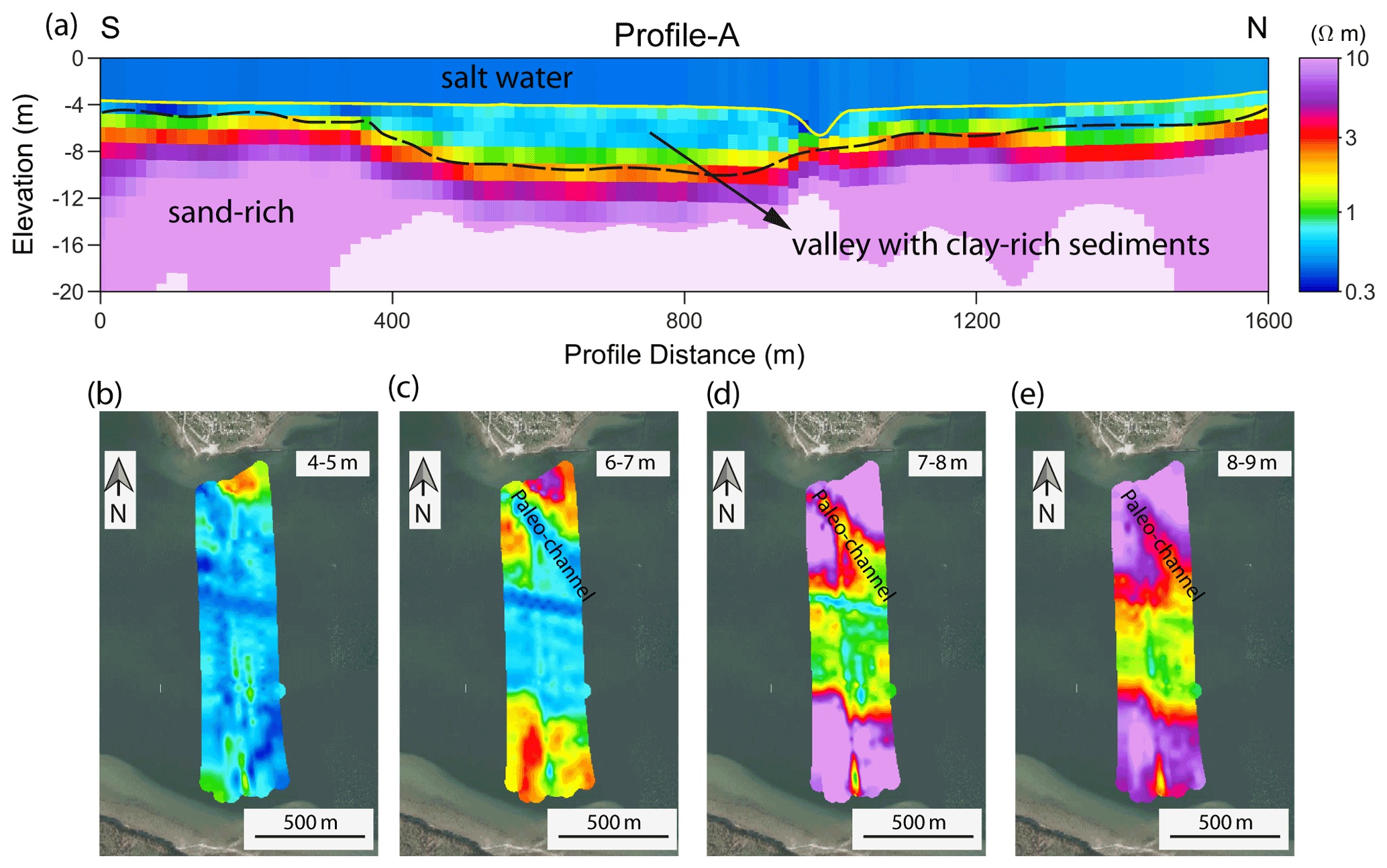
Figure 9Resistivity mapping results from Horsens bay. (a) Resistivity section (location marked in Fig. 8) with the seafloor marked with the yellow line. (b–e) Mean resistivity maps at different depths.
The mean resistivity maps (Fig. 9b–e) show the spatial variability of the clay–till and sand-rich sediments at four depth intervals below the seawater label. We see that the sediment close to the coast has a higher resistivity than what is observed in the middle of the fjord. This might be a transition from a sandy sediment towards a more clay-rich environment in the middle of the fjord. The knowledge of extension of these sand-rich sediments from coast to the middle of the fjord helps us to locate the probable regions where groundwater may discharge into the fjord. Additionally, we also observe a small northwest-trending low-resistivity structure that indicates a paleo-channel, which has been confirmed by shallow-seismic data (not shown).
The resistivity of a surface water body can change over short distances, so inversions will often benefit from a spatially varying resistivity constraint or reference. The need for a priori water resistivity and depth is higher in the freshwater cases than the saltwater case. The high conductivity in saltwater environments usually results in a well-resolved water column, so a priori information is less important. While the current instrument is integrated with a depth-sounder, it is not difficult to fit it with a conductivity logger as well to supply relevant a priori values for the water column. We note that the choice of towing vessel is important as a larger vessel requires a longer towing distance.
In general, the data quality for FloaTEM is usually better than comparable land surveys as lakes and rivers are often far from interfering infrastructure, which means that a FloaTEM survey normally results in full data coverage without gaps from data culling.
FloaTEM data provide critical information regarding sub-lake or subsea geology. In the Lake Sunds example, an interpretation based on land data only with lithological boundaries interpolated across the lake would be quite erroneous by missing the unique features associated with the genesis of the lake. The FloaTEM system provides a means of capturing these features which would be infeasible to identify with boreholes.
The depth of investigation is highly dependent on not only the resistivities of soils but also on the conductivity of the waters as the synthetic modeling study showed, where even a small conductivity change in the saltwater can reduce the DOI significantly. This stresses that a priori information about water salinity values is critical in selecting between the FW-FloaTEM and SW-FloaTEM configurations and designing the particular survey.
The high signal level in conductive saltwater environments often results in very low noise, also at the latest recorded time gate at ∼2 ms. In these cases, increasing the recording time and reducing the repetition rate should increase the DOI by adding more late-time data. However, a lower repetition rate may also lead to higher motion-induced noise in the receiver coil, which can become the dominating noise for the late-time gates.
The results shown here all focused on delineation of hydrological permeable (sands) and impermeable (clays) lithologies in the context of improving large-scale hydrological understanding and prediction strength. Although, from the given examples, it should be clear that the application range of FloaTEM spans much more. A few examples include foundation investigations for offshore wind farms, raw material exploration beneath lakes and rivers, and geotechnical pre-investigations for cabling routes below water bodies.
We have developed a new towed, easily configurable floating TEM instrument, FloaTEM, and successfully applied the system to both freshwater and saltwater studies to investigate geology and hydrology beneath lakes and shallow seawater. The FloaTEM system is modular, so longer beams can be used to increase the transmitter moment and likewise more transmitter turns can be added, both increasing the depth of investigation. Supported by synthetic analysis, we reconfigured a freshwater FloaTEM system to a saltwater FloaTEM system, primarily by increasing the transmitter moment and decreasing the noise in the receiver coil, enabling us to perform FloaTEM surveys not only on both shallow and deep lakes but also on shallow saltwater up to 8 m deep.
The conductance of the water (water depth multiplied with water conductivity) is the limiting factor when surveying on saline water. Based on the presented analysis, the water column should be below ∼25 S for the system to penetrate the water column and map underwater layers. For freshwater lakes and rivers, depths of investigation of 80 m or more are possible, while in saltwater cases we can achieve depths of investigation of 10–25 m strongly depending on water depth and conductivity.
With the FloaTEM system, we can map geological layers beneath the water bodies, which are normally not accessible for mapping with ground-based geophysical methods, thereby allowing for detailed hydrological modeling in these often-important areas as well. Through two freshwater cases and one saltwater case, we show the system's ability to image the heterogeneous geology beneath water bodies. In the freshwater cases the FloaTEM datasets revealed geological information that would have been impossible to deduce from land-based-only information, and in the saltwater case the data delivered clear images of the clay–sand distribution beneath the seafloor.
A1 Data processing and inversion
In this section, we give an overview of the data processing and inversion scheme used for FloaTEM data. In each of the case studies, FloaTEM data were processed with the Aarhus Workbench software from Aarhus GeoSoftware (https://www.aarhusgeosoftware.dk/, last access: 27 May 2022). The standard FloaTEM processing flow follows Auken et al. (2009). Raw data are first processed to remove coherent coupling interference due to nearby infrastructure and then stacked to produce soundings with approximately 10 m spacing. In the presented cases, a short smoothing filter was applied to the recorded water depth data, but this step depends on the quality of the depth-sounder data at hand. A preliminary inversion is then performed to evaluate and adjust the first-step processing of raw data.
The final inversions of the FloaTEM data were carried out using a spatially constrained inversion formulation, SCI (Viezzoli et al., 2009), using a 30-layer smooth model with layer thicknesses of layers 2–30 increasing logarithmically down to 120 m. The thickness of layer 1 is set to the water depth with a tight prior constraint. No vertical resistivity constraints are applied from the water layer (layer 1) to the sub-layers (layers 2–30), thereby allowing a shape boundary at the lake bed or seabed in the inversion results. The water depth prior information can be taken from the echo-sounder data or from an external bathymetry grid. Additionally, prior constraints can be added to the resistivity of the water layer if separate measurement of the water conductivity are present. In some cases, it is insufficient to model the water column as one homogeneous layer, e.g., probably due to a halocline or thermocline. In these cases, more layers are introduced to represent the water column in the inversion setup, and the prior water depth is assigned to the depth to the bottom of the last water layer.
Figures A1 and A2 show, respectively, examples of FW-FloaTEM and SW-FloaTEM data. Data in Figs. A1 and A2 correspond to the resistivity model along profile BB′ in Fig. 7 and resistivity model along profile A in Fig. 9, respectively. In each of the profiles, we selected three representative decay curves (see panels b–d in Figs. A1 and A2) and corresponding data fit. The quality of data fit is represented as data residual (see Auken et al., 2018), and it is generally below 1. In the SW-FloaTEM system, we ignored the early-time negative gates resulting due to offset geometry and very high conductivity of the saltwater.
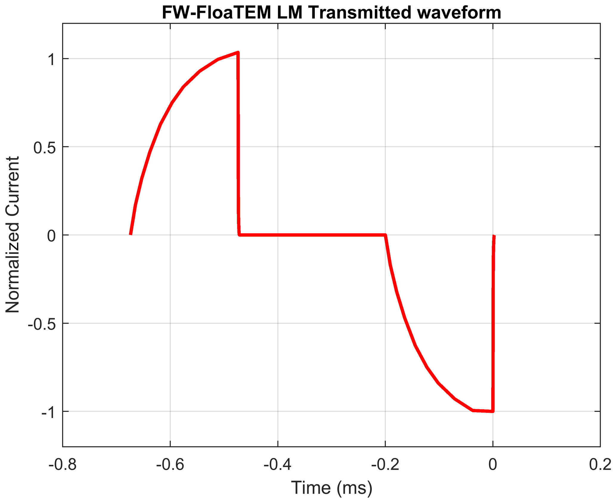
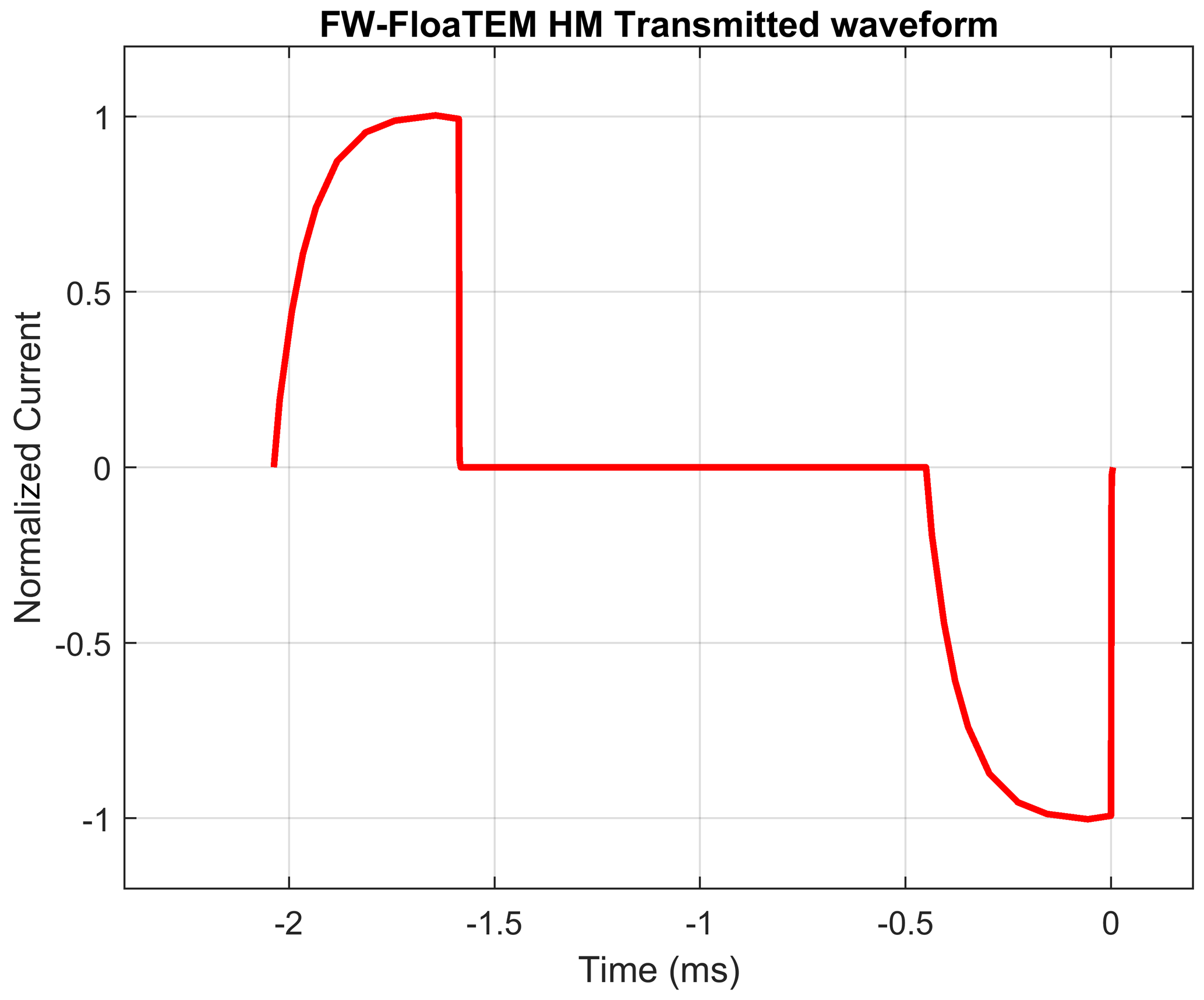
A2 Waveform of FW-FloaTEM and SW-FloaTEM systems
In the following figures (Figs. A3–A5), we show the transmitted waveforms for both low-moment (LM) and HM pulses used in the FW-FloaTEM system and only the HM waveform for the SW-FloaTEM system. For each waveform, we show both positive and negative pulses.
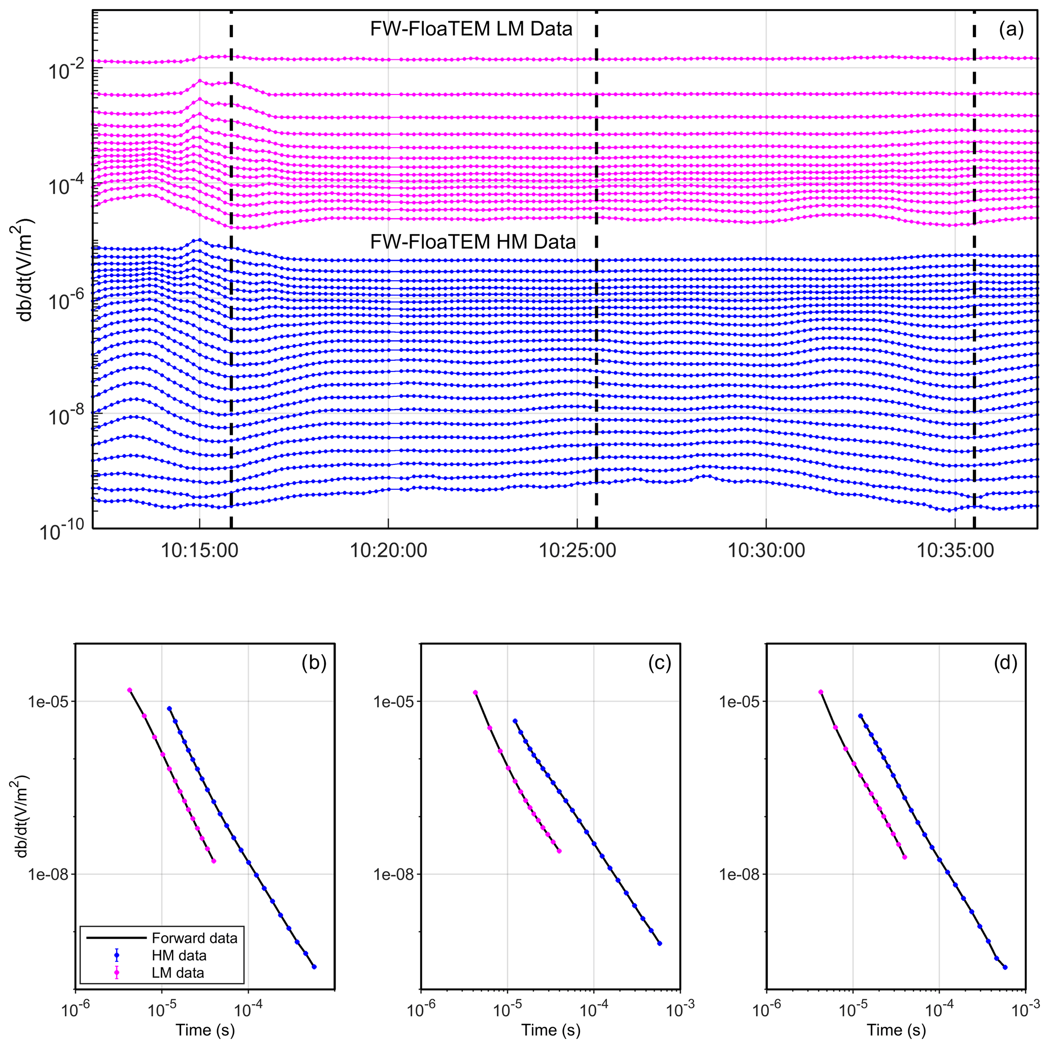
Figure A1An example of data acquired using the FW-FloaTEM system. Panel (a) shows the TEM data in profile view where each profile represents a gate; panels (b–d) show the transient decays shown, respectively, at three times marked as three vertical dashed lines in (a).
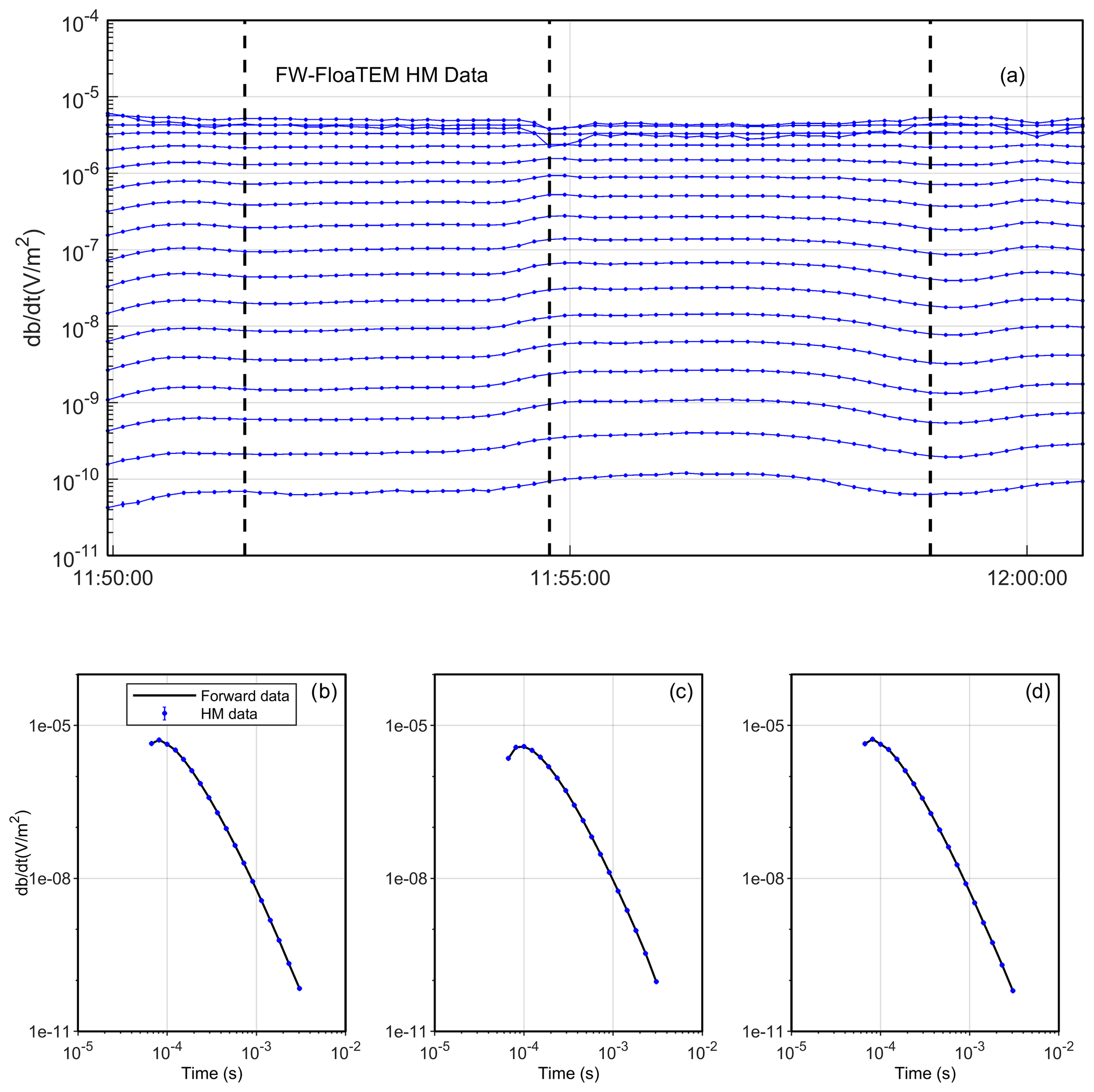
Figure A2An example of data acquired using the SW-FloaTEM system. Panel (a) shows the data in profile view where each profile represents a gate; panels (b–d) show the transient decays shown, respectively, at three times marked as three vertical black dashed lines in (a).

Data and code are available upon request to the corresponding author.
PKM designed and developed the methodology, instrumentation, data processing, and inversion and wrote the first draft of the article. FEC carried out data collection and data analyses and contributed to the original article. JBP and MAK contributed to the first draft of the article and to interpretations and feedback on inversion results. RRF provided data interpretations and feedback and contributed to the writing of original article. NF carried out synthetic data analysis and field data inversion for Ravnsø. AVC and EA conceptualized the methodology, contributed to writing the original article, and provided feedback.
The contact author has declared that neither they nor their co-authors have any competing interests.
Publisher's note: Copernicus Publications remains neutral with regard to jurisdictional claims in published maps and institutional affiliations.
We thank TOPSOIL, an Interreg project supported by the North Sea Region Programme of the European Regional Development Fund of the European Union. Partial support for data collection and interpretation of results was provided by GEUS (Geological Survey of Denmark and Greenland).
The development has been funded by Innovation Fund Denmark, project rOpen (“open landscape nitrate retention mapping”) and MapField (“field-scale mapping for targeted N-regulation”), WATEC (Aarhus University Centre for Water Technology), and internal HGG (HydroGeophysics Group at Aarhus University).
This paper was edited by Roberto Greco and reviewed by Shuangmin Duan and Craig William Christensen.
Auken, E., Jørgensen, F., and Sørensen, K. I.: Large-scale TEM investigation for groundwater, Explor. Geophys., 33, 188–194, 2003.
Auken, E., Christiansen, A. V., Westergaard, J. A., Kirkegaard, C., Foged, N., and Viezzoli, A.: An integrated processing scheme for high-resolution airborne electromagnetic surveys, the SkyTEM system, Explor. Geophys., 40, 184–192, 2009.
Auken, E., Christiansen, A. V., Fiandaca, G., Schamper, C., Behroozmand, A. A., Binley, A., Nielsen, E., Effersø, F., Christensen, N. B., Sørensen, K. I., Foged, N., and Vignoli, G.: An overview of a highly versatile forward and stable inverse algorithm for airborne, ground-based and borehole electromagnetic and electric data, Explor. Geophys., 46, 223–235, 2015.
Auken, E., Foged, N., Larsen, J., Lassen, K., Maurya, P., Dath, S., and Eiskjær, T.: tTEM – A towed transient electromagnetic system for detailed 3D imaging of the top 70 m of the subsurface, Geophysics, E13–E22, https://doi.org/10.1190/geo2018-0355.1, 2018.
Binley, A. and Kemna, A.: DC Resistivity and Induced Polarization Methods, in: Hydrogeophysics, edited by: Rubin, Y. and Hubbard, S. S., Springer Netherlands, Dordrecht, 129–156, https://doi.org/10.1007/1-4020-3102-5_5, 2005.
Briggs, M. A., Nelson, N., Gardner, P., Solomon, D. K., Terry, N., and Lane, J. W.: Wetland-Scale Mapping of Preferential Fresh Groundwater Discharge to the Colorado River, Groundwater, 57, 737–748, https://doi.org/10.1111/gwat.12866, 2019.
Christiansen, A. V., Auken, E., and Sørensen, K. I.: The transient electromagnetic method, in: Groundwater Geophysics. A tool for hydrogeology, 1st Edn., edited by: Kirsch, R., Springer, 179–224, https://doi.org/10.1007/3-540-29387-6_6, 2006.
Christiansen Vest, A. and Auken, E.: A global measure for depth of investigation, Geophysics, 77, WB171–WB177, 2012.
Danielsen, J. E., Auken, E., Jørgensen, F., Søndergaard, V., and Sørensen, K. I.: The application of the transient electromagnetic method in hydrogeophysical surveys, J. Appl. Geophys., 53, 181–198, 2003.
Day-Lewis, F. D., White, E. A., Johnson, C. D., Lane, J. W., and Belaval, M.: Continuous resistivity profiling to delineate submarine groundwater discharge – examples and limitations, Leading Edge, 25, 724–728, https://doi.org/10.1190/1.2210056, 2006.
Dickey, K. A.: Geophysical investigation of the Yellowstone Hydrothermal System, Geophysics, Virginia Tech, 110 pp., 2018.
Fitterman, D. V. and Deszcz-Pan, M.: Helicopter EM mapping of saltwater intrusion in Everglades National Park, Florida, Explor. Geophys., 29, 240–243, https://doi.org/10.1071/EG998240, 1998.
Gustafson, C., Key, K., and Evans, R. L.: Aquifer systems extending far offshore on the US Atlantic margin, Scient. Rep., 9, 1–10, 2019.
Harvey, J. and Gooseff, M.: River corridor science: Hydrologic exchange and ecological consequences from bedforms to basins, Water Resour. Res., 51, 6893–6922, https://doi.org/10.1002/2015WR017617, 2015.
Hatch, M., Munday, T., and Heinson, G.: A comparative study of in-river geophysical techniques to define variations in riverbed salt load and aid managing river salinization, 75, WA135–WA147, https://doi.org/10.1190/1.3475706, 2010.
Hinsby, K., Markager, S., Kronvang, B., Windolf, J., Sonnenborg, T. O., and Thorling, L.: Threshold values and management options for nutrients in a catchment of a temperate estuary with poor ecological status, Hydrol. Earth Syst. Sci., 16, 2663–2683, https://doi.org/10.5194/hess-16-2663-2012, 2012.
Jørgensen, F., Møller, R. R., Sandersen, P. B., and Nebel, L.: 3-D geological modelling of the Egebjerg area, Denmark, based on hydrogeophysical data, GEUS Bull., 20, 27–30, 2010.
Kwon, H.-S., Kim, J.-H., Ahn, H.-Y., Yoon, J.-S., Kim, K.-S., Jung, C.-K., Lee, S.-B., and Uchida, T. J. E. G.: Delineation of a fault zone beneath a riverbed by an electrical resistivity survey using a floating streamer cable, Explor. Geophys., 36, 50–58, 2005.
Lane, J. W., Briggs, M. A., Maurya, P. K., White, E. A., Pedersen, J. B., Auken, E., Terry, N., Minsley, B., Kress, W., LeBlanc, D. R., Adams, R., and Johnson, C. D.: Characterizing the diverse hydrogeology underlying rivers and estuaries using new floating transient electromagnetic methodology, Sci. Total Environ., 740, 140074, https://doi.org/10.1016/j.scitotenv.2020.140074, 2020.
Manheim, F. T., Krantz, D. E., and Bratton, J. F.: Studying Ground Water Under Delmarva Coastal Bays Using Electrical Resistivity, Groundwater, 42, 1052–1068, https://doi.org/10.1111/j.1745-6584.2004.tb02643.x, 2004.
Maurya, P. K., Christiansen, A. V., Pedersen, J. B., and Auken, E.: High resolution 3D subsurface mapping using a towed transient electromagnetic system – tTEM: case studies, Near Surf. Geophys., 18, 249–259, https://doi.org/10.1002/nsg.12094, 2020.
Meier, H., Edman, M., Eilola, K., Placke, M., Neumann, T., Andersson, H. C., Brunnabend, S.-E., Dieterich, C., Frauen, C., and Friedland, R.: Assessment of uncertainties in scenario simulations of biogeochemical cycles in the Baltic Sea, Front. Mar. Sci., 6, 46, https://doi.org/10.3389/fmars.2019.00046, 2019.
Micallef, A., Person, M., Haroon, A., Weymer, B. A., Jegen, M., Schwalenberg, K., Faghih, Z., Duan, S., Cohen, D., and Mountjoy, J. J.: 3D characterisation and quantification of an offshore freshened groundwater system in the Canterbury Bight, Nat. Commun., 11, 1–15, 2020.
Minsley, B. J., Rigby, J. R., James, S. R., Burton, B. L., Knierim, K. J., Pace, M. D. M., Bedrosian, P. A., and Kress, W. H.: Airborne geophysical surveys of the lower Mississippi Valley demonstrate system-scale mapping of subsurface architecture, Commun. Earth Environ., 2, 131, https://doi.org/10.1038/s43247-021-00200-z, 2021.
Mollidor, L., Tezkan, B., Bergers, R., and Löhken, J.: Float-transient electromagnetic method: in-loop transient electromagnetic measurements on Lake Holzmaar, Germany, Geophys. Prospect., 61, 1056–1064, https://doi.org/10.1111/1365-2478.12025, 2013.
Munk, L., Hynek, S., Bradley, D. C., Boutt, D., Labay, K. A., and Jochens, H.: Lithium brines: A global perspective: Chapter 14, Econ. Geol., 18, 339–365, https://doi.org/10.5382/Rev.18.14, 2016.
Nyboe, N. S. and Sørensen, K. I.: Noise reduction in TEM: Presenting a bandwidth- and sensitivity-optimized parallel recording setup and methods for adaptive synchronous detection, Geophysics, 77, E203–E212, 2012.
Ong, J. B., Lane, J. W., Zlotnik, V. A., Halihan, T., and White, E. A.: Combined use of frequency-domain electromagnetic and electrical resistivity surveys to delineate near-lake groundwater flow in the semi-arid Nebraska Sand Hills, USA, Hydrogeol. J., 18, 1539–1545, https://doi.org/10.1007/s10040-010-0617-x, 2010.
Parsekian, A. D., Singha, K., Minsley, B. J., Holbrook, W. S., and Slater, L.: Multiscale geophysical imaging of the critical zone, Rev. Geophys., 53, 1–26, https://doi.org/10.1002/2014RG000465, 2015.
Pihlainen, S., Zandersen, M., Hyytiäinen, K., Andersen, H. E., Bartosova, A., Gustafsson, B., Jabloun, M., McCrackin, M., Meier, H. M., and Olesen, J. E.: Impacts of changing society and climate on nutrient loading to the Baltic Sea, Sci. Total Environ., 731, 138935, https://doi.org/10.1016/j.scitotenv.2020.138935, 2020.
Rey, D. M., Walvoord, M. A., Minsley, B., Rover, J., and Singha, K.: Investigating lake-area dynamics across a permafrost-thaw spectrum using airborne electromagnetic surveys and remote sensing time-series data in Yukon Flats, Alaska, Environ. Res. Lett., 14, 025001, https://doi.org/10.1088/1748-9326/aaf06f, 2019.
Rumph Frederiksen, R. and Molina-Navarro, E.: The importance of subsurface drainage on model performance and water balance in an agricultural catchment using SWAT and SWAT-MODFLOW, Agr. Water Manage., 255, 107058, https://doi.org/10.1016/j.agwat.2021.107058, 2021.
Sandersen, J. F.: Kortlægning af begravede dale i Danmark, Opdatering 2015, GEUS Særudgivelse, http://begravededale.dk/PDF_2015/091116_Rapport_Begravede_dale_BIND_1_Endelig_udgave.pdf (last access: 27 May 2022), 2016.
Sheets, R. and Dumouchelle, D.: Geophysical Investigation Along the Great Miami River From New Miami to Charles M. Bolton Well Field, Cincinnati, Ohio, US Geological Survey, https://doi.org/10.3133/ofr20091025, 2009.
Siemon, B., Christiansen, A. V., and Auken, E.: A review of helicopter-borne electromagnetic methods for groundwater exploration, Near Surf. Geophys., 7, 629–646, 2009.
Sophocleous, M.: Interactions between groundwater and surface water: the state of the science, Hydrogeol. J., 10, 52–67, 2002.
Viezzoli, A., Auken, E., and Munday, T.: Spatially constrained inversion for quasi 3D modelling of airborne electromagnetic data – an application for environmental assessment in the Lower Murray Region of South Australia, Explor. Geophys., 40, 173–183, 2009.
Winter, T. C., Harvey, J. W., Franke, O. L., and Alley, W. M.: Ground Water and Surface Water A Single Resource, US Geological Survey, 1139, https://doi.org/10.3133/cir1139, 1998.
- Abstract
- Introduction
- The FloaTEM system
- Model resolution study
- Field cases
- Discussion
- Conclusions
- Appendix A: Examples of data processing and current waveforms of FloaTEM systems
- Code and data availability
- Author contributions
- Competing interests
- Disclaimer
- Acknowledgements
- Financial support
- Review statement
- References