the Creative Commons Attribution 4.0 License.
the Creative Commons Attribution 4.0 License.
 | 01 Jun 2022
Effects of spatial and temporal variability in surface water inputs on streamflow generation and cessation in the rain–snow transition zone
Ernesto Trujillo
Andrew Hedrick
Scott Havens
Katherine Hale
Mark Seyfried
Stephanie Kampf
Sarah E. Godsey
Climate change affects precipitation phase, which can propagate into changes in streamflow timing and magnitude. This study examines how the spatial and temporal distribution of rainfall and snowmelt affects discharge in rain–snow transition zones. These zones experience large year-to-year variations in precipitation phase, cover a significant area of mountain catchments globally, and might extend to higher elevations under future climate change. We used observations from 11 weather stations and snow depths measured from one aerial lidar survey to force a spatially distributed snowpack model (iSnobal/Automated Water Supply Model) in a semiarid, 1.8 km2 headwater catchment. We focused on surface water input (SWI; the summation of rainfall and snowmelt on the soil) for 4 years with contrasting climatological conditions (wet, dry, rainy, and snowy) and compared simulated SWI to measured discharge. A strong spatial agreement between snow depth from the lidar survey and model (r2 = 0.88) was observed, with a median Nash–Sutcliffe efficiency (NSE) of 0.65 for simulated and measured snow depths at snow depth stations for all modeled years (0.75 for normalized snow depths). The spatial pattern of SWI was consistent between the 4 years, with north-facing slopes producing 1.09–1.25 times more SWI than south-facing slopes, and snowdrifts producing up to 6 times more SWI than the catchment average. Annual discharge in the catchment was not significantly correlated with the fraction of precipitation falling as snow; instead, it was correlated with the magnitude of precipitation and spring snow and rain. Stream cessation depended on total and spring precipitation, as well as on the melt-out date of the snowdrifts. These results highlight the importance of the heterogeneity of SWI at the rain–snow transition zone for streamflow generation and cessation, and emphasize the need for spatially distributed modeling or monitoring of both snowpack and rainfall dynamics.
- Article
(5608 KB) - Full-text XML
-
Supplement
(1882 KB) - BibTeX
- EndNote


Due to increases in temperature, mountainous regions will receive less snowfall and more rainfall (Barnett et al., 2005; Stewart, 2009). This will alter the timing and amount of snowmelt, which is a significant source for water resources across the globe (Barnett et al., 2005; Marks et al., 1999; Somers and McKenzie, 2020; Viviroli et al., 2007). On the scale of the continental United States (US), a decrease in the fraction of precipitation falling as snow (snowfall fraction hereinafter) is expected to decrease stream discharge (Berghuijs et al., 2014). Earlier stream discharge peaks in response to earlier snowmelt and a decline in summer low flows across the semiarid mountainous US have been reported in both observational data records (McCabe et al., 2017; Luce and Holden, 2009; Regonda et al., 2005) and future climate projections (Naz et al., 2016; Leung et al., 2004; Milly and Dunne, 2020; Christensen et al., 2004). However, lower snowfall fractions in much of the western US have not yet led to a significant decrease in annual discharge (McCabe et al., 2017). Therefore, understanding year-round discharge responses, in particular the sensitivity of stream discharge to changes in yearly snowfall fractions, is warranted and will help us to anticipate how stream discharge might be affected by climate change.
Variations in snowfall fractions can affect the temporal distribution of surface water inputs (SWI = rainfall + snowmelt onto the soil). Snowpacks store water and release snowmelt later, whereas rain on snow-free ground immediately enters the rest of the hydrologic system. After rainfall or snowmelt reaches the ground surface, it might become stream discharge, remain stored on the land surface or in the soil, recharge deeper groundwater, or become evaporated or transpired. Generally, water inputs from rain or snowmelt during periods with high antecedent wetness and low evapotranspiration rates are more likely to recharge groundwater and generate discharge (Jasechko et al., 2014; Molotch et al., 2009; Hammond et al., 2019). Rainfall and snowmelt inputs might result in similar runoff ratios (discharge SWI) as long as the overall catchment wetness is similar or if the catchment is wet at key locations for water transport (Seyfried et al., 2009). The relationship between discharge and antecedent wetness conditions may reflect the ability of catchment storage to provide a “memory effect” of past inputs that can buffer short-term changes in inputs. However, this memory varies among catchments and across years (depending, for instance, on the local subsurface storage capacity or yearly variations in evapotranspiration), so that changes in snowfall fractions might not always affect stream discharge. Prevailing climatic conditions and subsurface storage capacity might also influence how precipitation is partitioned after it reaches the ground surface (Hammond et al., 2019), indicating that both the temporal and spatial distribution of SWI are important when considering how snowfall fractions affect seasonal to annual stream discharge generation.
Snowfall fractions may also influence the spatial distribution of SWI. In the semiarid western US, rainfall magnitudes generally increase with elevation (Johnson and Hanson, 1995). In regions with large snowfall fractions, this general elevation-driven pattern can be overlain by impacts of wind-driven redistribution of snow, which is dependent on factors such as topography, aspect, wind speed, and wind direction (Sturm, 2015; Tennant et al., 2017; Winstral and Marks, 2014; Trujillo et al., 2007). Hence, differences in the SWI distribution due to varying snow depths could be particularly substantial in areas where wind-driven redistribution of snowfall is significant. The primary controls (e.g., topography, aspect, and elevation) on snow depth and snow water equivalent (SWE) are relatively consistent from year to year, so the interannual distribution of snow is usually spatially consistent (Parr et al., 2020; Sturm, 2015; Winstral and Marks, 2002). The effects of elevation and aspect on the spatial distribution of snow depth and, thus, the potential for SWI as snowmelt, have been well studied in both high- and mid-altitude mountains (e.g., Grünewald et al., 2014; López-Moreno and Stähli, 2008; Tennant et al., 2017). Studies on snow drifting in seasonally snow-covered areas (Mott et al., 2018), prairie and arctic environments (e.g., Fang and Pomeroy, 2009; Parr et al., 2020), and in the context of avalanches (e.g., Schweizer et al., 2003) have shown that snowdrifts can strongly influence the spatial water balance. These studies have also revealed that Equator-facing slopes might only receive half as much SWI as snowmelt compared with snowdrift areas (Flerchinger and Cooley, 2000; Marshall et al., 2019). In turn, water originating from snowdrifts can locally control groundwater level fluctuations (Flerchinger et al., 1992) and contribute to streamflow into the summer season (Chauvin et al., 2011; Hartman et al., 1999; Marks et al., 2002). The relative importance of spatial snowmelt patterns is expected to increase with snowmelt magnitude, which is sensitive to snowfall fractions. Hence, quantifying spatial snowmelt patterns in areas that are not seasonally snow covered, as well as determining the importance of snowdrifts for streamflow generation in these areas, could be an important step in clarifying how stream discharge is affected by snowfall fractions.
One area where the snowfall fraction varies substantially from year to year is the rain–snow transition zone. The rain–snow transition zone is an elevation band in which the dominant phase of winter precipitation shifts between snow and rain (Nayak et al., 2010), and it is often characterized by a transient snowpack in (at least) parts of the defined area. Multiple studies in the European Alps and the northwestern US have shown that snowfall fractions in the rain–snow transition zone are particularly vulnerable to increases in temperature associated with climate change (e.g., Stewart, 2009). For example, towards the end of the century the snowfall fraction in the Swiss Alps is projected to decrease by about 50 % at ∼2000 m and by about 90 % at ∼1000 m. The current extent of the rain–snow transition zone covers about 9200 km2 in the Pacific Northwest of the US alone (here defined as Oregon, Washington, Idaho, and the western part of Montana; Nolin and Daly, 2006), and it is expanding and moving to higher elevations in response to climate change (Bavay et al., 2013; Nayak et al., 2010). This migration of the transition zone can affect precipitation patterns as well as discharge generation and timing across mountain ranges, with notable effects at the elevations surrounding the transition zone.
In addition to the expected decrease in snowfall fractions with climate change, annual climate variations are expected to increase almost everywhere across the planet (Seager et al., 2012), affecting annual runoff efficiency (Hedrick et al., 2020) and likely also influencing stream discharge timing and magnitude. One well-documented discharge response is that years in which catchments receive less snow have earlier snow-driven discharge peaks (McCabe and Clark, 2005; Stewart et al., 2005). This is relevant because earlier spring snowmelt has been linked to an increased risk of wildfire for catchments across the western US (Westerling et al., 2006) as well as to earlier and lower low-flows in the late-summer and fall months (Kormos et al., 2016). In some catchments and years, portions of the stream network might also completely cease to flow, and this drying can alter the network's ecological and biogeochemical functioning (Datry et al., 2014). In mid-elevation rain–snow transition zones, the annual snowpack variability is already relatively large. For example, in the Reynolds Creek Experimental Watershed (RCEW; Idaho, USA) the coefficient of variation (CV) of peak snow-water equivalent (SWE) between 1964 and 2006 ranged from 0.28 to 0.37 for five high-elevation stations (2056–2162 m) and was 0.72 for a mid-elevation weather station at the rain–snow transition zone (1743 m; Nayak et al., 2010). This mid-elevation variability suggests that year-to-year differences in snowfall at the rain–snow transition zone might already be substantial compared with nearby catchments at higher elevations, and it allows for the investigation of catchment hydrologic responses to snowfall variations using a relatively short data record, especially at sites where precipitation inputs are likely to be strongly reflected in stream discharge (i.e., with a limited memory of past inputs). Using observations of hydro-climatically different years (e.g., rainy vs. snowy) could reveal how discharge and stream drying at the rain–snow transition zone has responded to past variations in water inputs, thereby providing insight into how other small (<10 km2) catchments with a similar vegetation cover and precipitation regime might respond to future changes in rain–snow apportionments.
Thus, the overarching goal of this work is to improve our understanding of discharge responses to year-to-year variations in precipitation phase and magnitude. We do this at the rain–snow transition zone – a region that experiences large year-to-year variations in snowfall fractions, covers a significant part of the land surface, and might extend to higher elevations due to climate change. Specifically, we address the following research questions:
-
How does the spatial and temporal distribution of SWI at the rain–snow transition zone vary between particularly wet, dry, rainy, or snowy years?
-
How does stream discharge timing and amount respond to SWI in wet, dry, rainy, or snowy years?
-
Are variations in stream discharge related to variations in yearly snowfall fractions?
Examining natural variation in snowfall fractions in the rain–snow transition zone contrasts with other studies on snow-related processes that focus on seasonally snow-covered catchments. While many studies of snowmelt runoff examine seasonal responses at the landscape scale, here we focus on hourly responses at a fine spatial resolution. This allows us to investigate the spatial distribution of the snowpack and snowmelt as well as the phase of precipitation and the temporal distribution of SWI. Furthermore, while SWE is frequently used as a summarizing variable for winter precipitation when comparing precipitation to stream discharge, SWI is more directly related to the timing and amount of water resources; therefore SWI might be an important variable to model in future work addressing similar questions.
Our study location is Johnston Draw, a 1.8 km2 headwater catchment at the Reynolds Creek Experimental Watershed (RCEW) in Idaho, USA. Elevations range from 1497 to 1869 m a.s.l., and the mean annual air temperature and precipitation are 8.1 ∘C and 609 mm, respectively (2004–2014; Godsey et al., 2018a). Previous research in RCEW has shown that mid-elevation catchments (1404 and 1743 m a.s.l.) have seen an increase in minimum daily temperatures (+0.57 ∘C per decade), reduced snowfall (−32 mm per decade), and a decrease in streamflow (−13.8 mm per decade) over the 1965–2006 data record, whereas there has been no change in total precipitation (Nayak et al., 2010; Seyfried et al., 2011). These streamflow trends are unlikely to have been driven by increased plant water use (caused by increased temperatures) because there is only a short time window (∼ weeks) in which plant leaf out occurs, and there is still sufficient soil water available in this water-limited environment (Seyfried et al., 2011). The catchment is underlain by granite bedrock (79 %), with some basalt (3 %) and tuffs (18 %) (Stephenson, 1970), and slightly deeper soils exist on the north-facing slopes, although the difference is not significant (1.31±0.56 m vs. 0.77±0.34 m, respectively, p value = 0.05; Patton et al., 2019). Annual average soil water storage on the north-facing slopes is larger than on the south-facing slopes, which is primarily due to the difference in soil depth and a later start of vegetation growth compared with south-facing slopes (Godsey et al., 2018a; Seyfried et al., 2021). Snowberry (Symphoricarpos), big and low sagebrush (Artemisia tridentate and Artemisia arbuscula, respectively), aspen (Populus tremuloides) groves, and wheatgrass (Elymus trachycaulus) characterize the north-facing slopes, whereas the south-facing slopes host Elymus trachycaulus, Artemisia arbuscula, mountain mahogany (Cercocarpus ledifolius), and bitterbrush (Purshia tridentate) (Godsey et al., 2018a). Discharge at the catchment outlet is non-perennial, and the stream at the catchment outlet typically flows from early November until mid-July (MacNeille et al., 2020).
3.1 Hydrometeorological and discharge data
We used hourly hydrometeorological data recorded at 11 weather stations throughout the catchment (Fig. 1; Godsey et al., 2018a). The stations are placed at 50 m elevation intervals on the north- and south-facing slopes, and they span a ∼300 m elevation range (1508–1804 m a.s.l.; see Marks et al., 2013, for a detailed description). Observations started in 2002, although some stations were placed only in 2005 or 2010, and some stations were decommissioned in 2017 (see Godsey et al., 2018a, for exact years). Air temperature, solar radiation, vapor pressure, and snow depth were measured at hourly intervals at each of the stations, and additional measurements of wind speed, wind direction, and precipitation were available at jd125, jd124, and jd124b. The snow depth time series were processed to remove gaps and unreliable measurements during storms, and they were smoothed over an 8 h window in most cases and a 40 h window under specific circumstances (Godsey et al., 2018a). Stream discharge data (Godsey et al., 2018a) were obtained with a stage recorder using a drop box weir at the watershed outlet (Pierson et al., 2001). Stage height was converted to discharge using a rating curve (Pierson and Cram, 1998), and discharge was frequently measured by hand to ensure high data quality (Pierson et al., 2001).
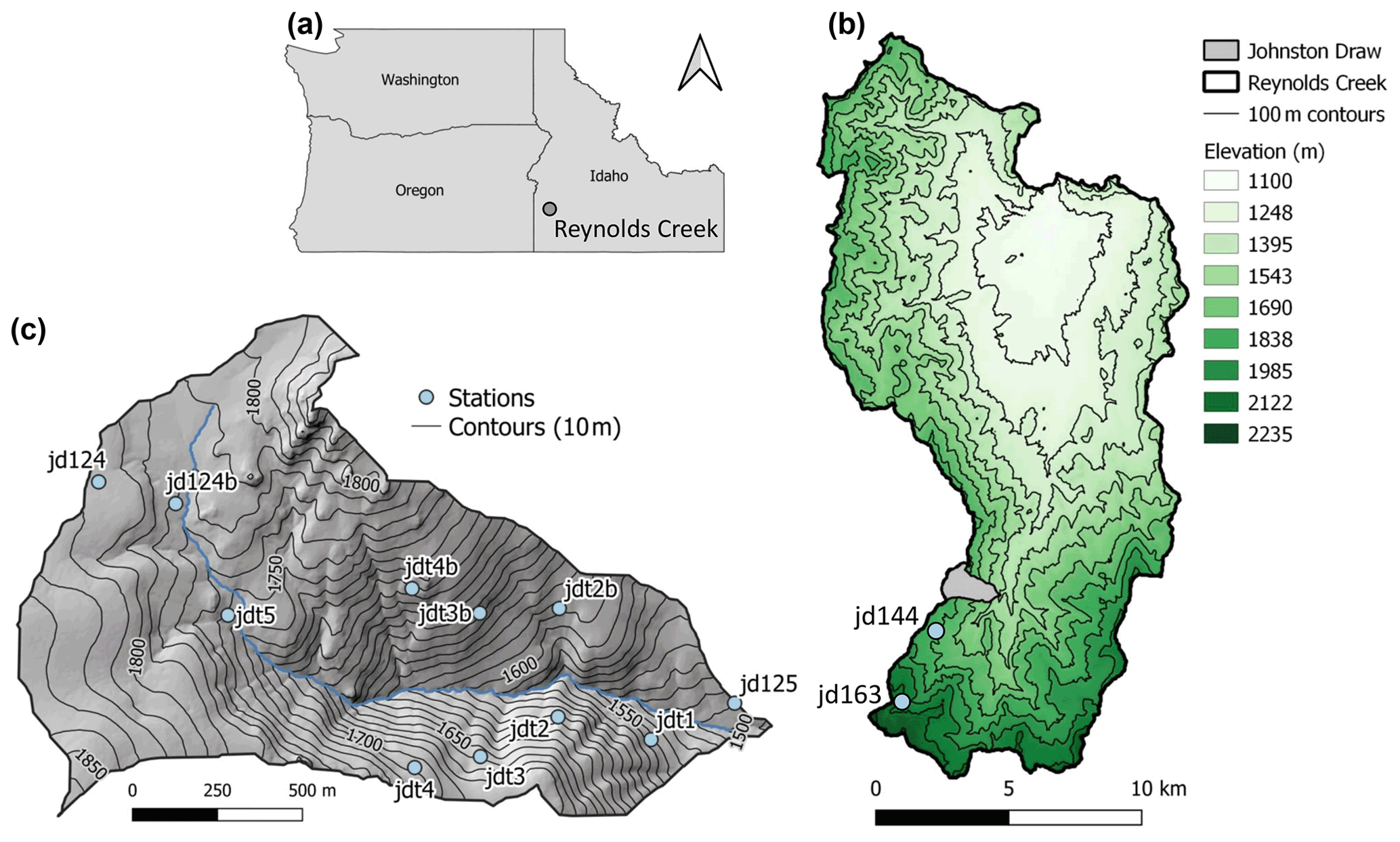
Figure 1Maps of the location of (a) the Reynolds Creek Experimental Watershed (RCEW) in the state of Idaho (USA; EPSG:4269 – NAD83 projection); (b) the Reynolds Creek Experimental Watershed showing the elevation (white – lower and dark green – higher), the 100 m contour lines, the location of Johnston Draw (gray polygon), and two additional precipitation gauges (light blue dots); and (c) Johnston Draw showing the weather stations (light blue dots), the stream (blue line), and the 10 m contour lines (black lines) overlain on a hillshade digital elevation model.
3.2 Remotely sensed observations
To characterize the spatial distribution of snow depth, a 1 m resolution snow depth product was calculated as the difference between a snow-off lidar flight (10–18 November 2007; Shrestha and Glenn, 2016) and a snow-on lidar flight (18 March 2009, around the time of peak accumulation), hereafter referred to as lidar snow depth. Typical vertical accuracies for lidar surveys are ∼10 cm (Deems et al., 2013). We assumed that uncertainties in both lidar surveys were uncorrelated, resulting in an overall uncertainty of ∼14 cm for lidar snow depth (summation in quadrature of uncertainties associated with each survey). All pixels that yielded a negative snow depth were excluded. The lidar snow depths were higher than the weather station snow depths, but this pattern was consistent across the catchment resulting in a strong linear relation between the two individual sets of snow depth measurements (r2 = 0.88; Fig. S1 in the Supplement).
Because only one lidar observation was available near peak snow accumulation, we also characterized snow presence throughout the season by mapping the snow-covered area (SCA) using satellite-derived surface reflectance at a 3 m resolution, which is available starting in 2016 (four-band PlanetScope scene; Planet Application Program Interface, 2017). This high-resolution imagery was critical for our analysis because snowdrifts in the rain–snow transition are relatively small in extent. No high-resolution satellite imagery was available for years that exhibited the key characteristics that we sought to study (e.g., rainy, snowy, wet, or dry; see Sect. 3.3), so we focused on a recent snow-covered period for which streamflow data and Planet imagery were available (1 November 2018 until 31 May 2019) to assess snow coverage. This targeted year was warmer than the year for which the lidar observations were available (mean annual air temperature of 8.0 ∘C, compared with 6.7 ∘C in 2009), which may have resulted in earlier peak streamflow, melt-out date, and dry-out date for the stream. We manually selected all available images in which the entire watershed was captured and for which snow was visually recognizable and then removed all images for which clouds significantly covered the watershed; this process resulted in 41 usable images. The information from all four spectral bands was then condensed to one layer using a principal component analysis (“RStoolbox” package in R). We used the Maximum Likelihood Classification tool in ArcMap (Esri Inc., 2020) to identify the SCA, after manually training the tool by selecting areas with and without snow cover (mean of 26 895 pixels per class and median of 9019 pixels), visually aided by the original satellite imagery. Obtaining training data was most challenging during periods in which almost the entire area was snow-free or covered with snow, for densely vegetated areas, and when part of the catchment was shaded. To overcome the latter, we classified “snow-free”, “snow-covered”, and “shaded snow” areas in heavily shaded images and, afterwards, merged “snow-covered” and “shaded snow” areas. The mean confidence for all classifications is shown in Fig. S2 in the Supplement. Our method differs from other satellite-derived snow products that combine both visible and infrared light, but it yielded a higher-resolution data product (3 m resolution vs. 30 m for Landsat 8 or 500 m for MODIS) that was necessary to capture the snowdrifts in the rain–snow transition zone.
We also used the surface reflectance imagery to determine the melt-out date of the snowpack for all years in which satellite and discharge observations were available (2016–2019). This was done by manually reviewing all available images and visually determining when all snow had melted. Given the high visiting frequency and limited cloudiness in early summer, we estimate that an error of ∼2 d is appropriate for these melt-out dates.
3.3 Spatially distributed snowpack modeling
We used the Automated Water Supply Model (AWSM; Havens et al., 2020) to obtain spatially continuous estimates of the distribution and phase of precipitation, snowpack characteristics, and surface water inputs (SWI). The two major components of the AWSM are the Spatial Modeling for Resources Framework (SMRF; Havens et al., 2017) and iSnobal (Marks et al., 1999). SMRF was used to spatially distribute precipitation and all other weather variables (air temperature, solar radiation, vapor pressure, precipitation, wind speed, and wind direction) along an elevation gradient using the hourly measurements from the weather stations. We included precipitation measurements from two stations within the basin (jd125 and jd124b) and two stations outside of the basin (jd144 and jd153; Fig. 1) to capture the elevation gradient. Precipitation at the wind-exposed site, jd124, was excluded because of precipitation undercatch issues. The interpolated vapor pressure and temperature fields were then used within SMRF to calculate the dew point and to further distinguish which fraction of precipitation fell as rain and/or snow. The output from SMRF was then used to force iSnobal, a physically based, two-layer snowpack model that accounts for precipitation advection from rain and snow (Marks et al., 1999).
The model was run at a 10 m resolution for 5 water years, namely 2005, 2009, 2010, 2011, and 2014. We selected 2009 because the snow depth lidar survey was available in this year, and we chose 2005, 2010, 2011, and 2014 because they are hydroclimatically different. The year 2005 was rainy (snowfall fraction was 63 % of the 2004–2014 mean and 23 % of 2005 total precipitation), whereas 2010 was snowy (snowfall fraction was 155 % of 2004–2014 mean and 57 % of 2010 total precipitation). The year 2014 was dry (precipitation was 86 % of the 2004–2014 mean) and 2011 was wet (precipitation was 132 % of the 2004–2014 mean) (Tables 1 and S3 and Fig. S4 in the Supplement) with snowfall fractions of 41 % and 30 % of the total precipitation for each year, respectively. The work was limited to 4 years because we aimed to focus on differences in the distribution of SWI and stream discharge for years that had different snowfall fractions and total precipitation magnitudes. Therefore, these strongly contrasting years were selected from 11 potential years of record (Godsey et al., 2018a). More stations were deployed towards the end of the 2004–2014 period, yielding additional observations to force the model with meteorological inputs and validate the model output of snow thickness; therefore, we selected later years within this period if conditions were similar. We focus on the 4 hydroclimatically distinct years in Sects. 4 and 5 of this paper, but we evaluate the model performance for all 5 years.
Table 1Precipitation, discharge, and SWI characteristics for each water year including total precipitation (average of precipitation measured at jd124b and jd125); the fraction of precipitation falling as snow (snowfall fraction); date and DOWY (day of water year) of the start of the snowy season (snowstart); date of the end of the snowy season (snowend), defined as <1 cm of snow at weather station jd124b (except for 2005, for which only data for weather station jd125 were available); date on which the simulated snow cover had melted (melt-out date; SCA = 0); annual discharge (Qannual); runoff efficiency (Qannual SWIavg); the start (Flowstart) and end (Flowend) of surface flow at the catchment outlet; and simulated surface water input (SWI). We report the catchment-average SWI (SWIavg) as well as SWI from rain (SWIrain), SWI from snowmelt (SWIsnow), the 98th percentile of SWI (SWI98), maximum SWI (SWImax), and the average SWI for north-facing slopes (excluding the drift area, SWINF−drift) and south-facing slopes (SWISF).
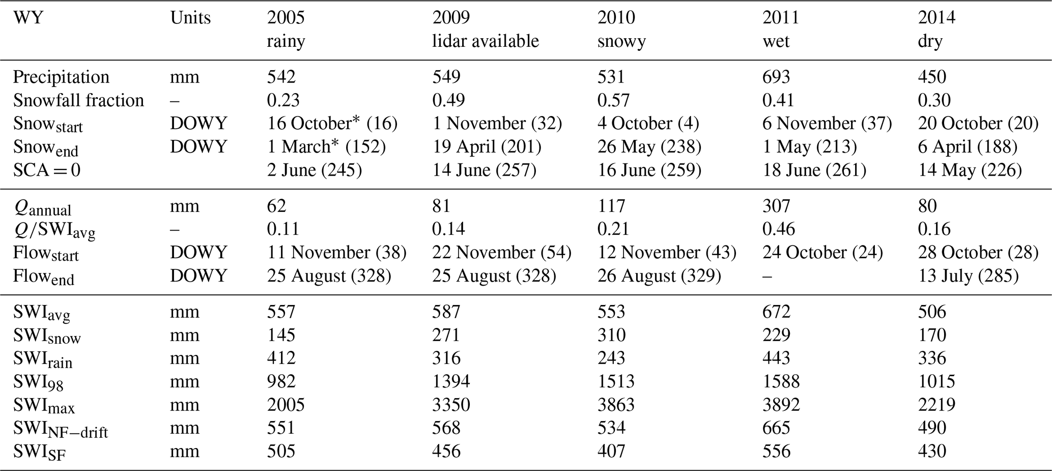
* Dates based on measurements at jd125 (outlet) rather than 124b (close to top of the catchment; see Fig. 1).
In order to represent the spatial variability in snowfall and the effects of wind redistribution of snow, we use the precipitation rescaling approach proposed by Vögeli et al. (2016) that implicitly captures the spatial heterogeneity induced by these processes using distributed snow depth information (e.g., from lidar or structure from motion (SfM)). This methodology can be used to rescale the precipitation falling as snow to reproduce the observed snow distribution patterns while conserving the initial precipitation mass estimation. Given the intra- and interannual consistency of spatial patterns of snow distribution (Pflug and Lundquist, 2020; Schirmer et al., 2011; Sturm and Wagener, 2010), Trujillo et al. (2019) extended the original implementation to utilize historical snow distribution information to other years in the iSnobal model. Following these successful implementations, we used the spatial distribution of snow depth from the 2009 survey around peak snow accumulation to inform the snowfall rescaling to all years in the study period. Although using the 2009 survey to rescale snowfall in other years might have induced some uncertainty, verification of the interannual consistency in the snow distribution in this catchment by comparing the lidar snow depth and the satellite imagery indicated that this uncertainty is likely to be small.
3.4 SWI
One of the model outputs from iSnobal is surface water input (SWI), which represents snowmelt from the bottom of the snowpack, rain on snow-free ground, or rain percolating through the snowpack. Rainfall is directly counted as SWI when it falls over snow-free ground, and it is included in the energy and water balances when it falls onto the snowpack. To calculate snowmelt, iSnobal solves each component of the energy balance equation for each model time step using the best available estimations of forcing inputs. Melt occurs in a pixel when the accumulated input energy is greater than the energy deficit (i.e., cold content) of the snowpack. If the accumulated energy input is smaller than the energy deficit, the sum of current hour melt and previous hour liquid water content will be carried over into the next hour. If that hour's input energy conditions are negative, the liquid mass is refrozen into the column. Sublimation and evaporation of liquid water from the snow surface and condensation of liquid water onto the snow surface is computed as a model output term, although these quantities were not considered here. Canopy interception must be handled a priori when developing the model forcing input, and it was also not considered here. Although not accounting for the latter introduces some uncertainty, we expect this to be small with the shrub and grass vegetation types in Johnston Draw catchment. Lastly, iSnobal is limited to snow processes only, which means that SWI “exits” the modeling domain. In reality, SWI travels to the stream as surface or subsurface runoff, could be stored in the soil until it evaporates or is transpired, or could recharge deeper groundwater storages. The route that SWI takes depends on the overall catchment wetness as well as the local energy balance (e.g., incoming radiation) and vegetation activity. In this paper, we computed SWI for each pixel and time step and assumed that all SWI generated in simulated snow-free pixels was rain and that all SWI generated in simulated snow-covered pixels was snowmelt.
3.5 Model evaluation
Model results were evaluated in two ways: first, the simulated snow depths were compared to lidar snow depths covering the entire basin on 18 March 2009; second, the temporal variation of the simulated snow depths were compared to snow depths measured at each of the weather stations for all simulated years. The latter comparison was done using model results from a 30 m × 30 m area surrounding each station; this is equivalent to 3×3 grid cells because the model was run at a 10 m resolution. We computed the root-mean-square error (RMSE) and Nash–Sutcliffe efficiency (NSE; Nash and Sutcliffe, 1970) for the observed vs. simulated snow depths as well as the NSE for the normalized observed vs. normalized simulated snow depths (NSEnorm). NSEnorm reflects the ability of the model to reproduce the dynamic behavior of the snowpack.
3.6 Comparison with discharge
The phase and magnitude of precipitation and the magnitude and temporal distribution of SWI were compared to annual discharge and the stream dry-out date. The stream dry-out date is the day when the stream first ceased to flow at the catchment outlet. For comparisons across seasons, we defined winter as December, January, and February; spring as March, April, and May; summer as June, July, and August; and fall as September, October, and November. To compare SWI with the dry-out date, we also calculated how much SWI occurred during the water year before the stream dried. No delays were considered when comparing SWI to discharge (e.g., discharge as a fraction of SWI in January results from dividing discharge in January by SWI in January). Discharge metrics were also compared to the flashiness of SWI inputs, which was calculated as the sum of the difference in total SWI from day to day, divided by the sum of SWI (also known as the Richards–Baker flashiness index; Baker et al., 2004). Further metrics included the fraction of time that more than half of the catchment was snow-covered as well as the melt rate between the date on which there was 40 % snow coverage in the catchment and the date on which the catchment was snow-free. A threshold of 40 % snow coverage was chosen because this resulted in an approximately linear melt rate for all years.
4.1 Snow depth observations
The lidar snow depth ranged from 0 to 5.3 m on the date of acquisition (18 March 2009), which was near peak snow cover (median of 0.4 m and CV of 0.91; Fig. 2a). The south-facing slopes had little to no snow cover (mean of 0.3 m), whereas the north-facing slopes were covered with 0.7 m of snow on average. For the years studied here, during the approximate duration of the snowy season between 15 November and 15 April, the average snow depth for all north-facing stations was more than 5 times that of the average snow depth at south-facing stations (0.20 vs. 0.04 m, respectively), and the snowpack lasted almost 90 d longer on average (132 vs. 43 d, respectively). Weather stations on north-facing slopes and at higher elevations generally had deeper snowpacks and were covered with snow for longer than sites on the south-facing slopes or at lower elevations (Godsey et al., 2018a). The snowpack distribution was also affected by wind-driven redistribution of snow. For instance, snow depths at jdt2 (north facing) and jdt3b (south facing) were consistently lower than at the weather stations directly below them in elevation (jdt1 and jdt2b, respectively). Large snowdrifts formed in some western parts of the watershed, up to a maximum depth of 5.3 m (90th percentile of all snow depths was 1.2 m; Fig. 2a). Wind-driven redistribution of the snow in Johnston Draw is facilitated by a relatively consistent southwesterly wind direction (average of 225∘ during storms) and high wind speeds (average of 6.7 m s−1 during storms at the wind-exposed station of jd124; Fig. S5 in the Supplement).
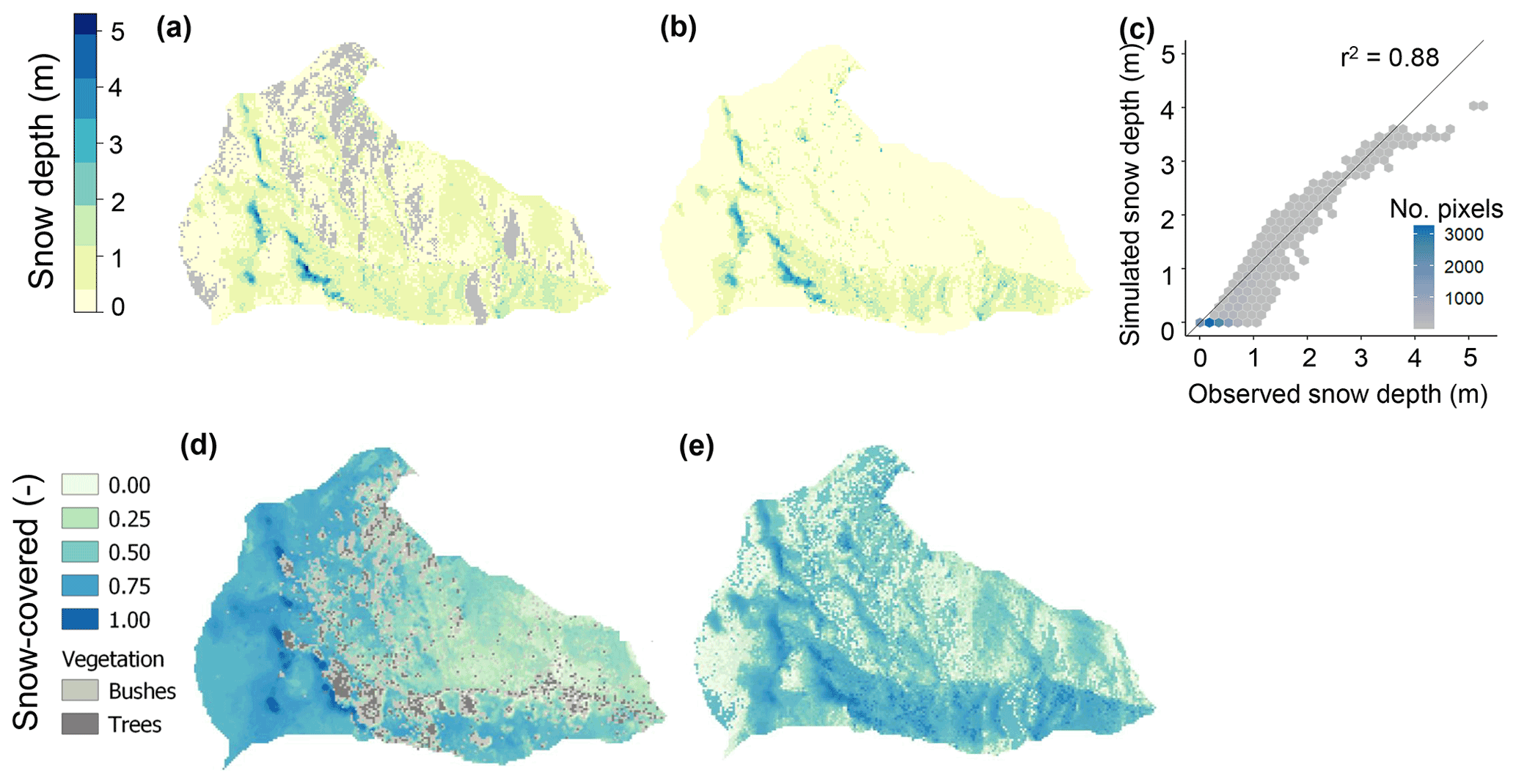
Figure 2(a) Lidar snow depth (m) at 3 m resolution on 18 March 2009 and (b) simulated snow depths for the same day, where yellow indicates low snow depths, blue indicates high snow depths, and gray indicates the areas for which the snow depth could not reliably be determined from the lidar measurement (see Sect. 3.2). (c) Hexagonal bin plot comparing the observed and simulated snow depths, with gray colors indicating fewer pixels and blue indicating more pixels included per bin. (d) The fraction of images for which sites were snow covered, using 3 m resolution satellite imagery for the available images (n=41) of water year 2019 (see Sect. 3.2), and (e) the fraction of time during which each pixel was snow covered, using the simulated snow cover from the beginning of water year 2009 until all snow had melted (n=238). Bushes and trees (marked in gray in panel d) inhibited the exact determination of the snow cover for the satellite imagery in some locations.
4.2 Snow depth model performance in space and over time
Simulated snow depths on the day of the lidar survey agreed well with the lidar snow depth (r2 = 0.88; Fig. 2a, b, c). The residual snow depths (lidar − simulation) were approximately normally distributed, with a mean of 0.2 m (see Fig. S6 in the Supplement for a histogram and quantile–quantile plot). The largest differences (maximum difference of 1.1 m) between the simulated and measured snowpack were for isolated 10 m pixels on both the north- and south-facing slopes (Fig. 2a, b, c). The spatial pattern of the lidar snow depth also agreed well with the spatial patterns of snow-covered area (Fig. 2a, d), and there was a strong agreement between the simulated snow-covered area for 2009 (Fig. 2e) and the snow-covered area determined from satellite imagery for 2019 (Fig. 2d), including the modeled duration of snow cover and the number of satellite images in which snow-covered areas were observed. The largest discrepancy between the simulated and imagery-based snow duration was in the scour zone west of the snowdrifts, where the model underestimated snow duration. Nonetheless, the consistent locations of the snowdrifts between 2009 (observed and simulated) and 2019 (observed) indicates that the model captured the spatial distribution of the snowpack.
The median NSE for the hourly simulated snow depths compared to observations at the weather stations ranged from 0.22 (wet 2011) to 0.86 (snowy 2010) for all modeled years and weather stations, with the RMSE ranging from 0.008 to 0.097 m (Table 2; see Fig. S7 in the Supplement for time series of all simulated and observed snow depths). The RMSE was equal to or lower than 0.1 m for all years, with the year in which the NSE performance was lowest (wet 2011) having an RMSE of 0.046 m. The temporal variation of the snowpack at each of the weather stations was well captured by the model; the median NSE for the normalized snowpack depths (NSEnorm) ranged from 0.65 to 0.94 (median of 0.75), although there were some sites and years with low NSE values (Table 2). Both high and low NSE values are observed at nearly all of the stations (e.g., the NSE range at jdt4 was from −9.60 to 0.91, and the range at jdt1 was from 0.01 to 0.83) with lower values at some sites in 2011. Possible explanations for the relatively low performance at the remaining sites are discussed further in Sect. 5.3. Despite the low performances for some years and locations, the normalized snow depths were largely acceptable (35 out of 40 year–location combinations had a NSEnorm value above 0.5; Table 2). The generally strong performance lends confidence that the simulation of ablation and accumulation processes in the model is reasonable and implies that the temporal distribution of snow-covered area (SCA) and surface water input (SWI) simulated by the model are reliable.
Table 2The Nash–Sutcliffe efficiency (NSE; Nash and Sutcliffe, 1970) and root-mean-square error (RMSE) for simulated and observed snow depths at each weather station as well as the NSE for normalized (z-transformed) snow depths (NSEnorm). Dashes (–) indicate that no observed snow depths were available in that year. See Fig. S7 in the Supplement for the time series of observed and simulated snow depths.

4.3 Spatial and temporal pattern of surface water inputs (SWI)
The spatial pattern of SWI was similar for all years, with the highest SWI occurring in the snowdrifts (maximum SWI (SWImax) was 3892 mm, and 98th percentile of SWI (SWI98) was 1235 mm, both in wet 2011; Fig. 3, Table 1). Annual SWI across the rest of the catchment varied less, with north-facing slopes receiving 45 to 127 mm more SWI than south-facing slopes (values for rainy 2005 and snowy 2010, respectively; Table 1). Snowdrift locations received 1.7 to 2.7 times more SWI than the catchment average (ratio SWI98 SWIavg). Summarizing SWI by aspect (see polar diagrams in Fig. 3) revealed the highest SWI on northeast-facing slopes and roughly equal annual SWI for all other aspects. Differences between the northeast-facing slopes and other parts of the catchment were largest in snowy 2010 (a ratio of the major / minor axis of the polar plot of 1.29) and smallest in rainy 2005 and dry 2014 (ratio of 1.13 and 1.17, respectively).
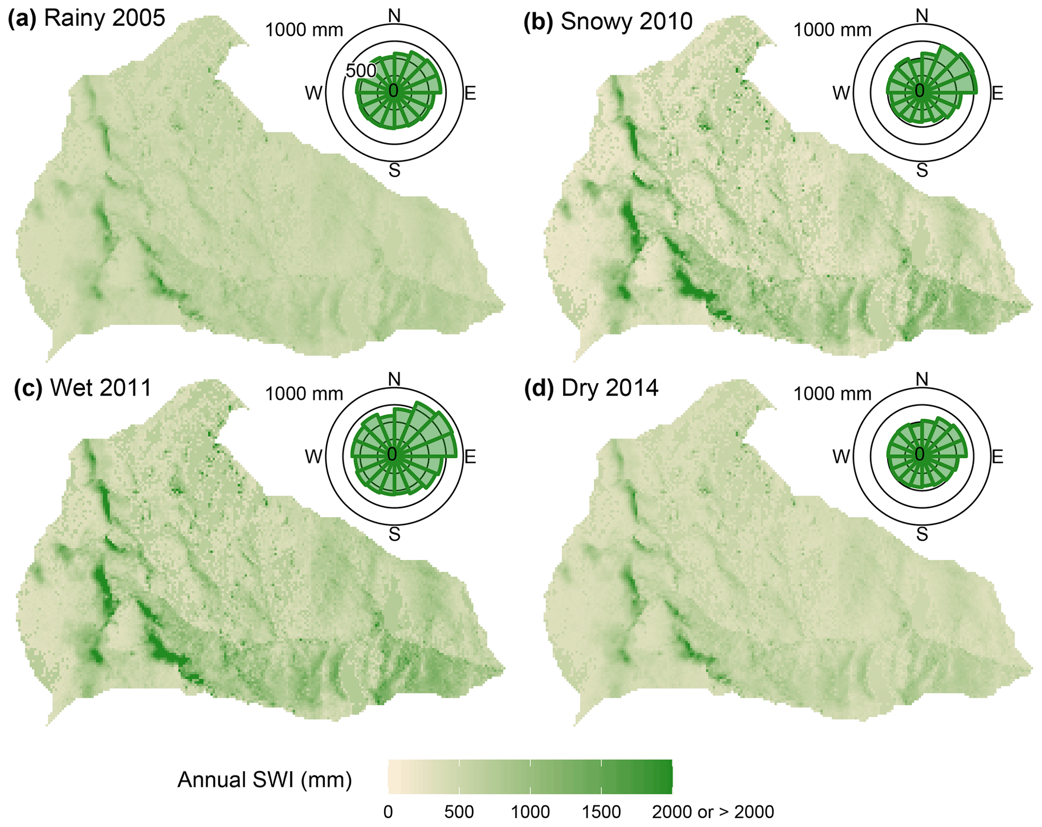
Figure 3Maps showing the yearly sum of surface water inputs (SWI, mm) for (a) rainy 2005, (b) snowy 2010, (c) wet 2011, and (d) dry 2014, with polar diagram insets showing the average sum of SWI per 10 m grid cell for each aspect (binned per 22.5∘). Higher SWI values are shown in darker colors, lower SWI values are shown in lighter colors, and SWI values are capped at 2000 mm to enhance the contrast. Maximum annual SWI values are shown in Table 1, and a map of simulated SWI for 2009 is shown in Fig. S13 in the Supplement.
Weekly sums of SWI ranged from 0 to ∼75 mm in all years (Fig. 4). Summer most frequently had weeks without SWI generation, whereas the highest weekly SWI occurred with simultaneous rainfall and snowmelt (i.e., rain-on-snow events, such as the one visible in February 2014 in Fig. 4d). However, large rainfall events without snowfall or snow cover in spring of rainy 2005 (weekly SWI of ∼75 mm) and in fall of wet 2011 (weekly SWI of ∼50 mm; gray peaks in Fig. 4a and c) also generated high SWI. In 2011, the majority of SWI was generated in winter and spring (47 % between December and May; see inset in Fig. 4c), whereas most SWI was generated in winter (54 % between December and February; Fig. 4d) in dry 2014. In 2005 and 2010, most SWI was generated in spring (March–May 32 % and 46 %, respectively). Similar amounts of SWI occurred in spring in 2005 and 2010 (339 and 388 mm, respectively); however, in 2005, 93 % came from rain, whereas only 35 % came from rain in 2010. Average daily spring SWI rates were higher in snowy 2010 than in rainy 2005 (mean spring SWI rate of 3.7 mm d−1 in 2010 vs. 2.9 mm d−1 in 2005). Overall, variations in weekly and daily SWI rates were lower in snowy 2010 (CV daily SWI of 1.71) than in all other years (2.50 in 2005, 2.14 in 2011, and 2.65 in 2014).
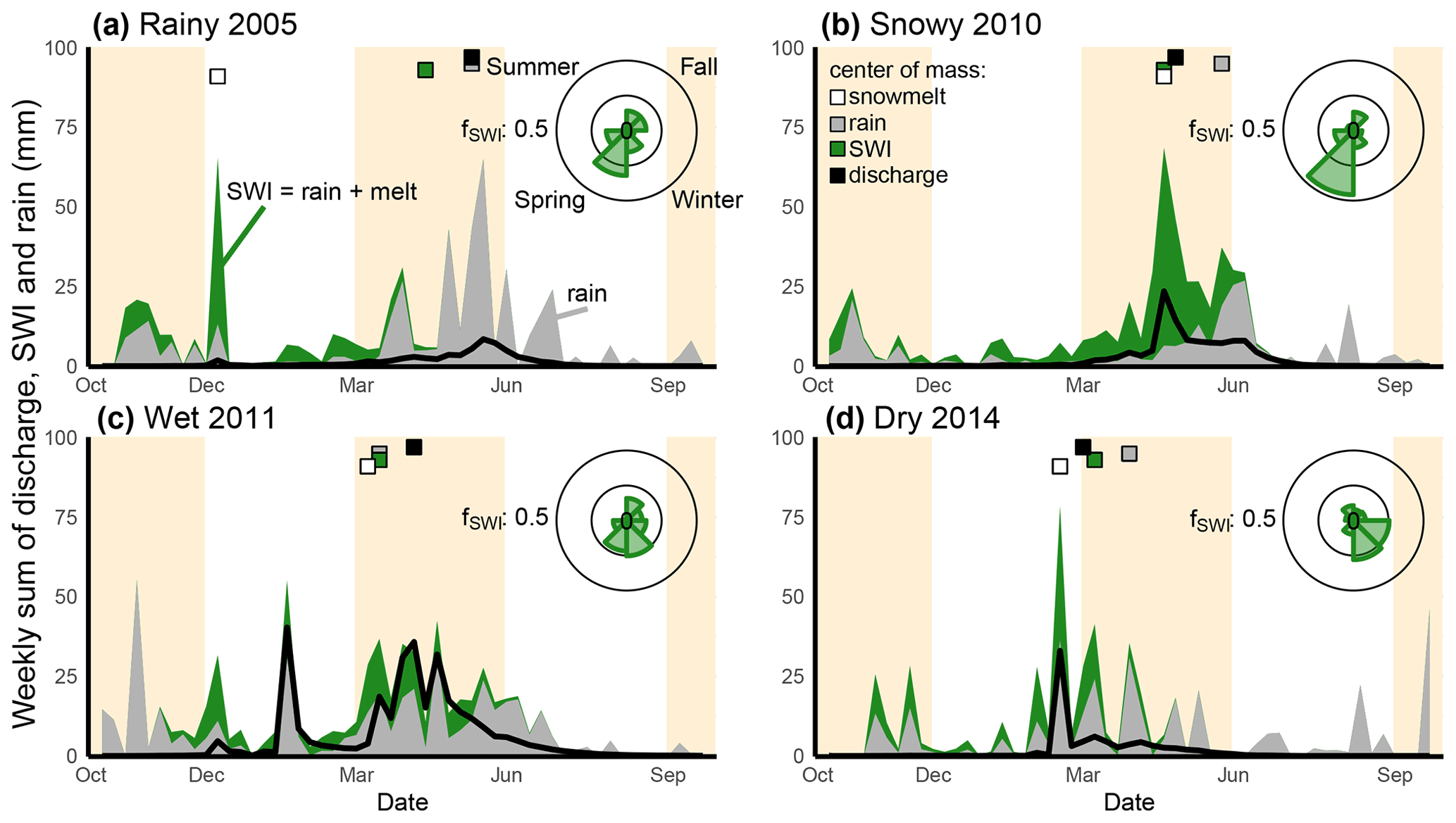
Figure 4Weekly sums of surface water inputs (SWI, summation of rainfall and snowmelt, green polygons, mm), rainfall (gray polygons, mm), and specific discharge (black line graph, mm) for (a) rainy 2005, (b) snowy 2010, (c) wet 2011, and (d) dry 2014. Background panels are colored according to the different seasons (fall, winter, spring, summer, fall). The polar diagram insets indicate the fraction of SWI (fSWI) in each season. Squares at the top of each panel indicate the annual center of mass for snowmelt (white), rainfall (gray), SWI (green), and discharge (black).
4.4 Stream discharge
Streamflow was least responsive to SWI at the beginning of each water year (Fig. 5). For instance, in 2005 and 2010, 174 and 108 mm of SWI occurred before 1 February (31 % and 20 % of annual SWI), whereas discharge amounted to only 7 % and 1 % of its yearly total during that same period. Similarly, 82 mm of SWI in October 2011 resulted in less than 1 mm discharge, whereas 180 mm of SWI in November–January led to 62 mm of discharge. SWI generally resulted in most discharge when SWI rates were high, such as during a 3 d rain-on-snow event in February 2014 (SWI of 75 mm and discharge of 29 mm) or during spring snowmelt in April 2011 (SWI of 108 mm and discharge of 102 mm). Such individual precipitation events had a strong influence on the annual runoff efficiency. For instance, 2014 had a slightly higher runoff efficiency (0.16) than 2005 (0.11) and 2009 (0.14), mostly due to the high runoff generation during one rain-on-snow event (29 mm, 36 % of yearly discharge).
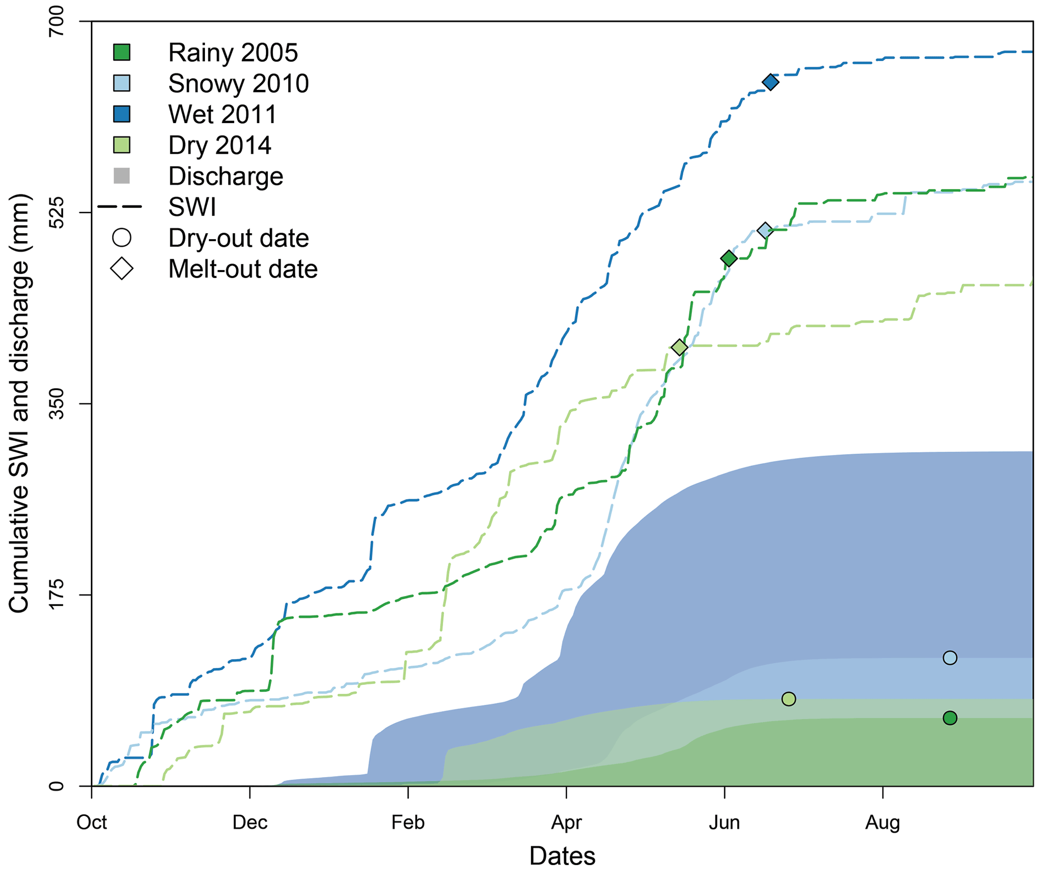
Figure 5Cumulative surface water inputs (SWI, dashed lines, mm) and discharge (colored polygons, mm) for each of the water years (dark green – rainy 2005, light blue – snowy 2010, dark blue – wet 2011, and light green – dry 2014). Circles indicate the day on which the stream ceased to flow at the catchment outlet (dry-out date; please note that the stream did not cease to flow in 2011), and diamonds indicate the day on which all snow had melted from the catchment (melt-out date).
Annual discharge was highest in 2011 (307 mm, 43 % of SWI) and lowest in 2005 (62 mm, 11 % of SWI). Despite similar SWI in 2005 and 2010 (SWIavg of 553 and 557 mm, respectively; Table 1), snowy 2010 had nearly twice as much annual discharge as rainy 2005 (117 mm or 21 % of SWI vs. 62 mm or 11 % of SWI, respectively). Apart from these 2 years, there was no relation between annual discharge and the annual snowfall fraction (Fig. 6c) nor between annual discharge and the amount of SWI produced by rainfall or snowmelt in different seasons (winter, spring, summer, or any combination of these periods). By considering additional years (for which SWI was not simulated), we found that annual discharge was positively related to the amount of precipitation recorded at the lowest-elevation precipitation station (jd125, r2=0.83; Fig. 6a). Annual discharge was slightly higher for years that were preceded by a year that received above average annual precipitation (see Fig. S8 in the Supplement), but the correlation coefficient decreased when including the precipitation totals recorded in the preceding year (e.g., annual discharge vs. precipitation in the same year + 0.5 times precipitation previous year). This indicates that any memory effect is likely to be small in this catchment. Frequent stream drying (16 out of 18 years between 2003 and 2020, data not shown; the stream did not cease flow in 2006 and 2011) and the high potential evaporation rates in this semiarid, high desert system (evapotranspiration accounts for nearly 90 % of precipitation in the nearby Upper Sheep Creek catchment; Flerchinger and Cooley, 2000) also suggest that any water in the shallow, “active” subsurface storage is likely limited and that any memory effect, if present, is perhaps constrained to deeper subsurface water storages.
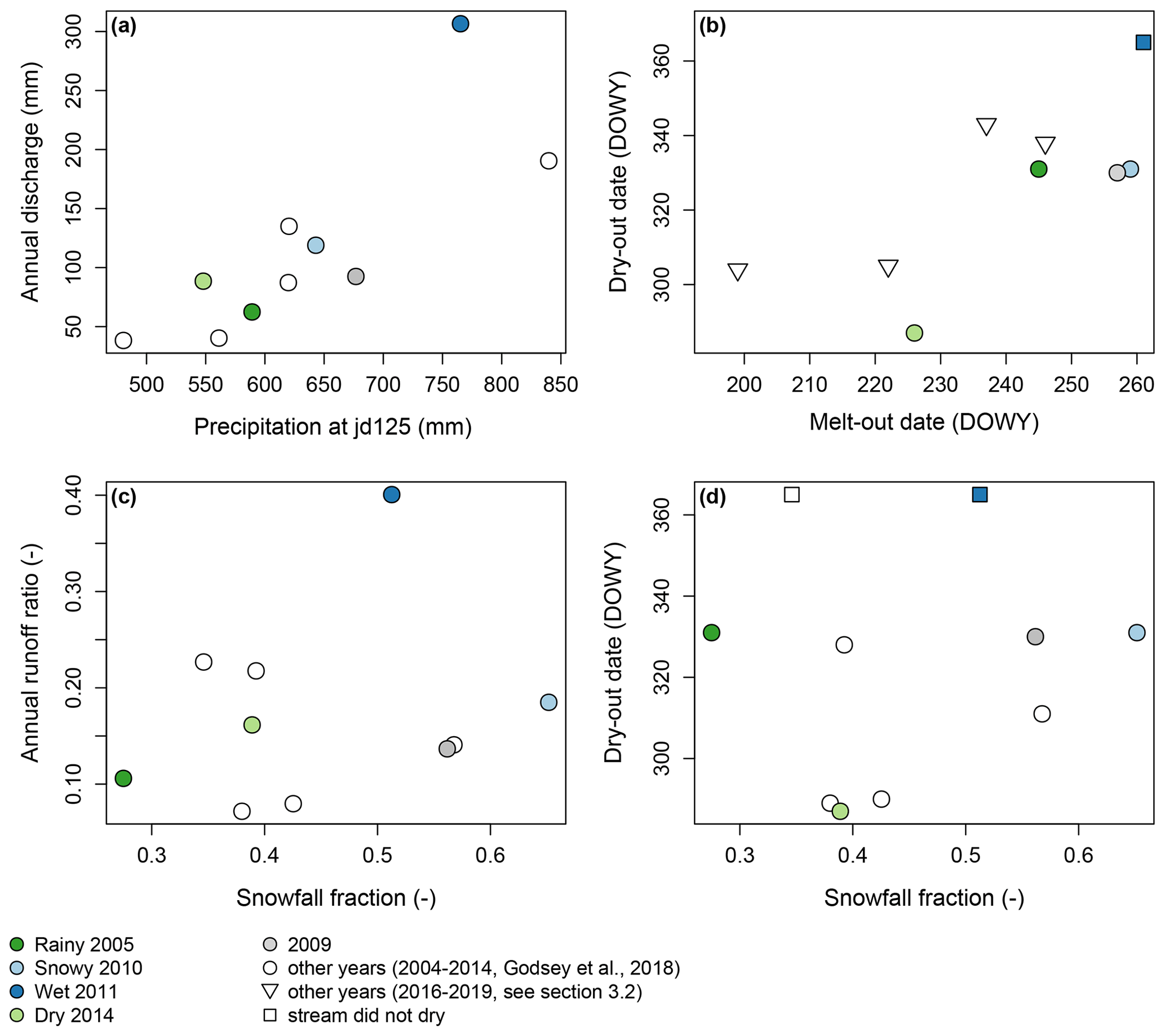
Figure 6Scatterplots of (a) annual discharge at the catchment outlet (mm) and annual precipitation at the lowest precipitation gauge (jd125, mm; see Fig. S14 in the Supplement for a comparison with simulated mean catchment precipitation), (b) the day that surface flow in the stream ceased (dry-out date, shown as day of water year – DOWY) and the day on which all snow had melted (melt-out date, DOWY), (c) the annual runoff ratio (annual discharge / annual precipitation at jd125) and the annual snowfall fraction (–), and (d) the stream dry-out date and the annual snowfall fraction. Years in which the stream did not dry out are projected to the last day of the hydrological year. The r2 and p values for linear regressions between the variables in each panel are (a) r2=0.83 and p value =0.001, (b) r2=0.74 and p value =0.023, (c) r2=0.23 and p value =0.524, and (d) r2=0.12 and p value =0.730.
Comparison of annual discharge and the stream dry-out date to metrics describing the phase and magnitude of precipitation, the temporal distribution of SWI, and key characteristics of the snowpack highlighted the importance of the magnitude and timing of SWI (Fig. 7). Significant relationships with annual discharge were found for annual precipitation (Fig. 6a) and the sums of precipitation and snowfall in spring (Figs. 7 and S9 in the Supplement). The dry-out date of the stream was significantly correlated with annual precipitation, the sum of winter and spring precipitation and spring snowfall, spring precipitation as a fraction of SWI, the melt-out date of the snowpack, and the sum of SWI before the dry-out date (Figs. 7 and S9 in the Supplement). No significant correlation was found between the annual, winter, and spring snowfall fraction and annual discharge and the stream dry-out date (Fig. 7).
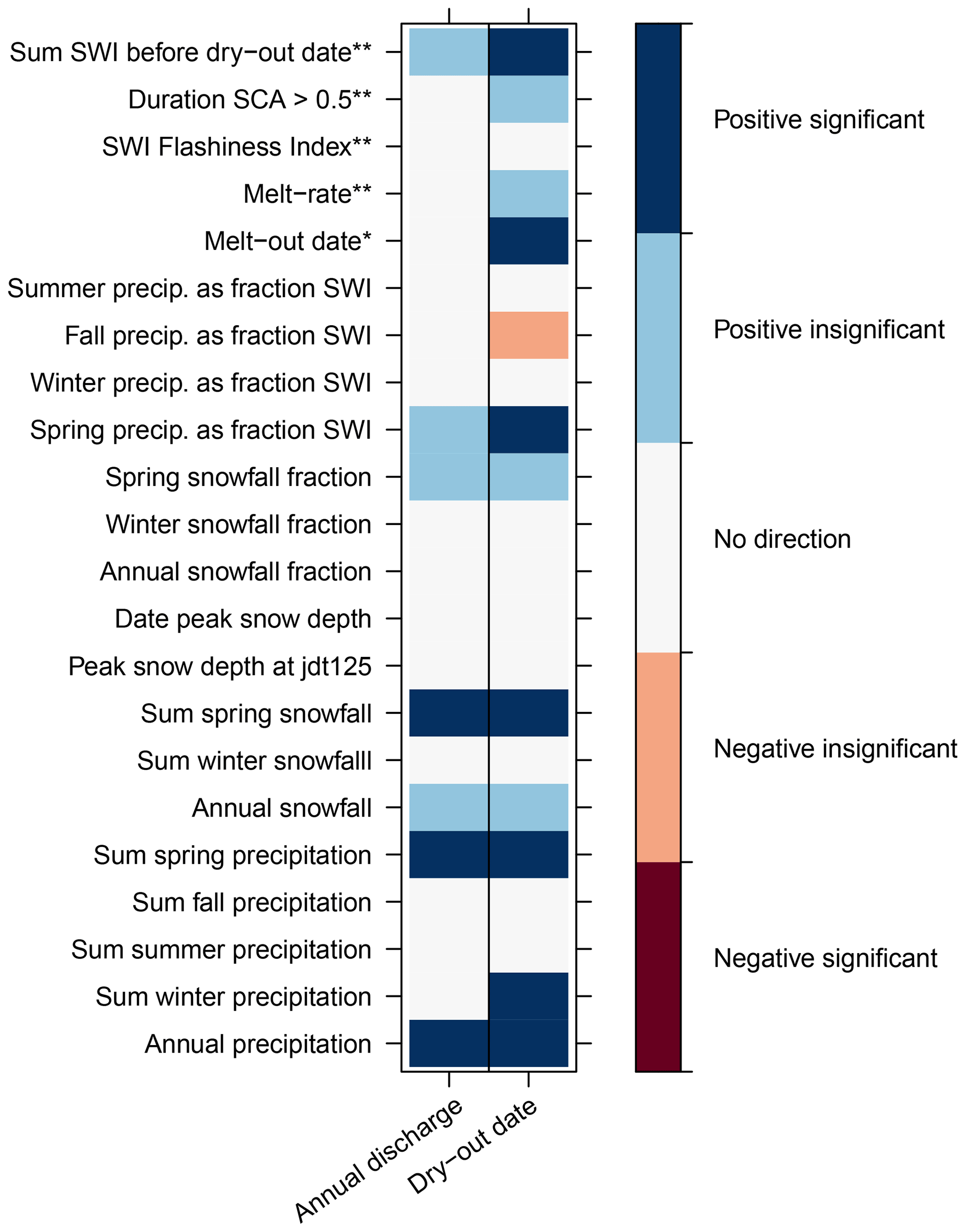
Figure 7Heat plot showing the Pearson correlation coefficients (α=0.1) for comparisons between annual discharge, the stream dry-out date, and precipitation and snowpack metrics. Significant correlations are marked in dark red (negative) and dark blue (positive), insignificant correlations are marked in light blue (positive) or light red (negative), and correlations without a direction are marked in white (r<0.3). For most metrics, the comparison is based on the 2004–2014 data record (n=11 years). The comparison with the melt-out date (marked with one asterisk) is based on the simulated years (n=5) and the years for which satellite imagery was available (2016–2019, n=4; which totals to n=9). For the SWI flashiness index, the melt rate, the number of days on which at least half the catchment was snow covered, and the sum of SWI before the dry-out date (marked with two asterisks), we used only the years that were simulated (n=5). Scatterplots of all significant correlations can be found in Fig. S9 in the Supplement.
5.1 Spatial variability in SWI
Snow drifting and aspect-driven differences in snow dynamics caused a strong variability in the spatial pattern of the snowpack (Fig. 2a) and SWI (Fig. 3). We found that the spatial pattern in simulated SWI was similar across all years, with snowdrifts receiving up to 7 times more SWI than the catchment average (SWImax SWIavg in 2010; Table 1). Even in rainy 2005, SWI was more than 3.5 times higher in the snowdrifts (SWImax of 2005 mm) compared with the catchment average (SWIavg of 573 mm; Table 1). In our modeling routine, the spatial consistency between years is pre-determined by the snowfall rescaling (see Sect. 3.3), but this likely also reflects real-world conditions, as suggested by the spatial agreement between the independently collected satellite imagery and lidar snow depths (Fig. 2). Most importantly, the nearly 4-fold variation in SWI over less than 1 km distance is equivalent to the average precipitation difference between most of Reynolds Creek and the peaks of the Cascade Mountains in Oregon hundreds of kilometers away or, equivalently, shifting from a semiarid steppe to coastal mountain snowpack. This difference directly affects water-limited processes such as weathering or plant species distribution. In Johnston Draw, this is clearly visible: aspen stands are located directly below snowdrifts (Kretchun et al., 2020), and sagebrush dominates the rest of the catchment. Because snowdrifts drive the spatial pattern of SWI, it is crucial to quantify wind-driven redistribution processes as well as capture aspect and elevation-driven processes, even at the rain–snow transition zone.
Snowdrifts delivered 4.2 % (2005) to 7.2 % (2010) of the basin-total annual SWI on just ∼2 % of the land surface, and snow in drifts persisted longer, compared with non-drift areas, into the spring season (Fig. 2d, e). Previous work in the seasonally snow-covered Reynolds Mountain East catchment showed that snowdrifts indeed hold a large fraction of total catchment snow water equivalent (SWE), with 50 % of total SWE on just 31 % of the catchment area (Marks et al., 2002), and SWI varying strongly in space, ranging from 150 to 1100 mm for individual grid cells (10–20 m) in the relatively dry water year 2003 (Seyfried et al., 2009). Snowdrifts in Johnston Draw were shallower (up to 5 m in 2009) and covered a smaller portion of the area (∼2 %) than in the higher-elevation Reynolds Mountain East catchment, but they were proportionally even more important in the rain–snow transition zone, holding up to 15 % of SWE during peak SWE in snowy 2010 and 25 % in rainy 2005. Water originating from snowdrifts has been shown to locally control groundwater level fluctuations (Flerchinger et al., 1992) and contribute to streamflow into the summer season (Chauvin et al., 2011; Hartman et al., 1999; Marks et al., 2002). For instance, in the Upper Sheep Creek watershed, also in RCEW, Chauvin et al. (2011) showed that the lowest stream discharge was recorded for the year in which snowdrifts were least prominent. In Johnston Draw, the stream dry-out date was positively correlated with the drift melt-out date (Fig. 6b), suggesting that isolated snow patches are also important at this location for sustaining streamflow. These results do not reveal the mechanism or influence of the specific drift location, as neither subsurface flow nor streamflow generation processes were measured or simulated. Nonetheless, observations of snowdrifts from high-resolution satellite imagery are largely consistent with model simulations of SCA (Fig. 2) and, thus, may be used to predict stream drying in drift-influenced watersheds.
5.2 Temporal variability in SWI and discharge response
We found that the majority of SWI occurred in winter and spring and that catchment-average SWI was more uniform in time in snowy 2010 than in the other years (CV of daily SWI in 2010 was 1.7, whereas other years ranged from 2.14 to 2.65). The steadier water inputs in the snowmelt period might explain why annual discharge in snowy 2010 was double that of rainy 2005 despite similar total SWI. More stable water inputs from snowmelt rather than flashy water inputs from rain could have led to wetter soils and higher soil conductivity rates, allowing more water to pass through the subsurface towards the stream or towards deeper storage (Hammond et al., 2019). Previous work in the nearby Dry Creek Experimental Watershed (Idaho) showed that water stored in the soil dries out approximately 10 d after snowmelt (McNamara et al., 2005). For the years on record here, streamflow was sustained for a minimum of 59 d after the melt-out date (Table 1), even though SWI is generally low after June each year (Fig. 4). This underscores that it is likely that deeper flow paths contribute to the stream in early summer. This is also consistent with stream discharge being nearly unresponsive to SWI during the dry catchment conditions in the beginning of each water year (Fig. 5). During fall, subsurface water storage across the catchment is low; thus, any SWI during this period likely results in recharge or evaporation rather than stream discharge (Seyfried et al., 2021). Air temperature also has a small effect on the runoff efficiency, particularly in the summer season. The runoff efficiency, calculated as summer discharge divided by summer precipitation for the 2004–2014 record, was significantly correlated with summer air temperatures (, p value = 0.08; Fig. S10 in the Supplement), whereas this relationship was insignificant on the annual scale (, p value = 0.217; Fig. S11 in the Supplement). This suggests that evapotranspiration, which is directly affected by the ambient air temperature, has some influence on runoff efficiency, despite the catchment being an overall water-limited environment. Warmer winter air temperatures result in higher runoff efficiencies (r2=0.48, p value = 0.131; Fig. S10 in the Supplement), which is likely due to faster melt-out and more saturated soils, as described above. However, further simulations are required to fully understand how precipitation amounts, timing, and location interact with subsurface water storage to control stream discharge.
In contrast with our hypothesis and what has been suggested in the literature (e.g., based on the comparison of 420 catchments in the continental US using the Budyko framework; Berghuijs et al., 2014), neither annual discharge nor the stream dry-out date were correlated with snowfall fraction (Figs. 6, 7). Instead, annual discharge and the stream dry-out date were more correlated with total precipitation and the snowpack melt-out date. This highlights the importance of the temporal distribution of SWI, which is not captured in an annual snowfall fraction. The temporal distribution of SWI might be less important for predicting stream discharge and cessation in more humid catchments (in which precipitation is more evenly distributed over the year and/or in which more precipitation events occur) or in larger catchments, such as those considered in Berghuijs et al. (2014; range of catchment areas between 67 and 10 329 km2). We found that individual precipitation events can also heavily influence the yearly runoff efficiency, as described for 2014 (Sect. 4.4). As such, considering interannual variability and rainfall or snowmelt events is an important addition to annual average values when investigating how precipitation affects discharge in semiarid regions.
Bilish et al. (2020) similarly found that streamflow was not correlated with the snowfall fraction for a small catchment with an ephemeral snowpack in the Australian Alps. They attributed this to the frequent occurrence of mid-winter snowmelt: the snowpack melted out several times each year, independent of the annual snowfall fraction, and, thus, did not store a significant amount of water. Field observations at Dry Creek, a nearby semiarid catchment that includes a rain-dominated and a snow-dominated area, also suggested that the snowfall fraction was not related to annual discharge for a small sub-catchment at the rain–snow transition zone (treeline sub-catchment, 0.015 km2), but the snowfall fraction was correlated with annual discharge when considering the entire Dry Creek catchment (28 km2, James McNamara, personal communication, 2021). Another study at Dry Creek suggested that the snowfall fraction is less important than spring precipitation to satisfy the evaporative demands of upland ecosystems (McNamara et al., 2005), emphasizing the importance of the temporal distribution of SWI for other semiarid catchments. For the years studied here, we found that streamflow was sensitive to spring precipitation and total precipitation but that the snowfall fraction did not significantly affect stream discharge (Figs. 6, 7).
5.3 Limitations and opportunities
Although the model adequately reproduced the spatial snowpack patterns and dynamics (Fig. 3 and Table 2), temporal variations in the snow depths (i.e., melt and accumulation) recorded at the weather station locations were simulated better than the absolute snow depths. To investigate why simulations of snow depths were poor for some stations and years, we calculated the average and precipitation-weighted average wind directions, wind speeds, and snow densities for all events during which the snowfall fraction was higher than 0.2 (i.e., 20 %; see Table S12 and Fig. S13 in the Supplement) from the station data. Although wind speed and directions were generally consistent (Fig. S13 in the Supplement), in 2011, the combination of higher snow densities (stronger cohesion of snow particles; 122 kg m−2) and lower wind speeds (less energy for transport; 5.7 m s−1) compared with 2009 (102 kg m−2 and 6.5 m s−1, respectively; precipitation-weighted averages in Table S12) might have led to less wind redistribution of snow in that year and correspondingly resulted in underpredictions of snow depths at north-facing and high-elevation sites in 2011 (jdt3, jdt4, jdt5, and jd124b). As NSE values are based on squared errors, the divergence between the simulated and observed snow depths impacted the model performance more severely in 2011 than in years with shallower snowpacks (i.e., 2005 and 2014). The snowpack density, wind speed, and wind direction values in 2005 diverged most from 2009, from which the lidar observations were used, but nonetheless had a relatively high performance (NSE = 0.83), possibly because data from only one station were available for validation.
In addition to the uncertainty in the spatial redistribution of snow depending on wind speeds, wind direction, and snow densities, we suggest three additional reasons for the differences between simulated and observed snow depths. First, the varying performance at jd125 might be related to inaccuracies in calculating the phase of precipitation, which would most strongly affect lower elevations at which the phase shifts more often from rain to snow. Any uncertainty in the magnitude or phase of precipitation would decrease model efficiency because precipitation was interpolated based on elevation, after which the proportion of precipitation falling as snow was redistributed based on the lidar snow depths (see Sect. 3.3). Second, the simulated snow depths reflect all processes occurring in each 10 m grid cell (our model resolution), whereas the ultrasonic snow depth measurements represent processes at ∼ 1–3 m2. Therefore, small differences between the simulated and observed snow depths are expected. Third, iSnobal is a mass and energy balance model; therefore, it is optimized to correctly model mass. Thus, model evaluation using snow depths (instead of SWE) is less favorable, as small differences in snow densities and SWE could lead to significant differences in snow depths. However, as snow depth measurements were available and SWE measurements were not, we focused on snow depth. Uncertainties were also present in the weather station snow depths as well as in the lidar-based snow depths and the satellite-based SCA analysis. We compared the spatial patterns from the lidar and satellite imagery to test if the spatial pattern was consistent between these two data sources and found this to largely be the case (Fig. 2). As such, we are confident that, despite the uncertainties of our analysis, we captured the within-catchment variability of the snowpack and also adequately modeled the variability in SWI that we set out to investigate.
Discrepancies between simulated and observed snow depths are challenging to solve, especially for areas with an ephemeral snow cover (Kormos et al., 2014) or with complex vegetation patterns, such as the sagebrush in Johnston Draw. Shallow snow covers are more sensitive to small variations in energy fluxes than deeper seasonal snow covers (Pomeroy et al., 2003; Williams et al., 2009). As a result, small errors in the spatial extrapolation of the forcing data or in the forcing data itself (e.g., uncertainty in the observed relative humidity or temperature) can introduce uncertainties in the model results (Kormos et al., 2014). For instance, the transition from snow-covered to snow-free areas results in a large change in albedo, which influences solar radiative fluxes. The snowpack at the rain–snow transition zone can melt out several times per year, even within a single day, and melt-out dates are variable across the catchment. Therefore, a small error in the simulated melt-out date for each cell can result in a larger error in the basin-average or yearly results. Perhaps these challenges are also a reason for the limited number of studies that have simulated warm snowpacks (Kormos et al., 2014; Kelleners et al., 2010), despite multiple regional studies highlighting that the rain–snow transition zone is expanding and that regional climates are changing rapidly (Klos et al., 2014; Nolin and Daly, 2006). Challenges linked to snow ephemerality likely also affected our results, but the agreement between the observed and simulated snow depths indicates that at least the general patterns of accumulation and melt in space and over time were represented by the simulations, at a scale that was small enough to characterize the snowdrifts.
Regardless of the challenges that come with studying an intermittent snow cover, the relationship between the snowpack melt-out date and stream dry-out date poses interesting opportunities to inform hydrological models or evaluate model results with independent observations. Measurements of SCA can be obtained through satellite imagery and are, thus, easier and cheaper to obtain than SWE or snow depth measurements (e.g., Elder et al., 1991). Satellite observations can be particularly helpful to investigate remote areas that exceed a feasible modeling domain, and they can be used to inform or evaluate models. Given the restrictions for satellite imagery imposed by clouds and the visit frequency, particularly for areas with an ephemeral snow cover that might melt out in a single day, a combination of satellite imagery and snowpack modeling seems a promising way to leverage these observations while ensuring the fine temporal resolution that might be needed to study stream cessation.
As a result of climate change, the rain–snow transition zone will receive more rain and less snow, which may influence the spatial and temporal distribution of surface water inputs (SWI, summation of rainfall and snowmelt). The goal of this work was to quantify the spatial and temporal distribution of SWI at the rain–snow transition zone as well as to assess the sensitivity of annual stream discharge and stream cessation to the temporal distribution of SWI and to the annual snowfall fraction. To this end, we used a spatially distributed snowpack model to simulate SWI during 5 years, of which 4 had contrasting climatological conditions. We found that the spatial pattern of SWI was similar between years and that snow drifting and aspect-controlled processes caused large differences in SWI across the watershed. Snowdrifts received up to 6 times more SWI than other sites, and the difference between SWI from the snowdrifts and catchment average SWI was highest for the year with the highest snowfall fraction. This highlights that the snowfall fraction affects the spatial variability in SWI, with more rain leading to less variability. The majority of SWI occurred in winter or spring, which was also the time that the percentage of SWI becoming streamflow was highest (up to 94 % in April 2011). Over the 2004–2014 data record, annual discharge was insensitive to snowfall fraction and depended more on total and spring precipitation. The stream dry-out date was also sensitive to total and spring precipitation. In addition, stream cessation was positively correlated with the last day on which there was snow present anywhere in the catchment, which indicates that the persistence of snowdrifts in small parts of the catchment is critical for sustaining streamflow. This study highlights the heterogeneity of SWI at the rain–snow transition zone, its impact on stream discharge, and, thus, the need to spatially and temporally represent SWI in headwater-scale studies that simulate streamflow.
The hydrometeorological and discharge data used in this paper are available at https://doi.org/10.15482/USDA.ADC/1402076 from Godsey et al. (2018b), satellite imagery can be obtained from Planet Application Program Interface (2017) (https://www.planet.com/), and the remaining data are available upon reasonable request.
The supplement related to this article is available online at: https://doi.org/10.5194/hess-26-2779-2022-supplement.
LK and SEG developed the concept for the study. LK, SH, ET, AH, and KH performed and/or contributed to the simulations. LK prepared the first draft of the manuscript. All co-authors provided recommendations for the data analysis, participated in discussions about the results, and edited the paper.
The contact author has declared that neither they nor their co-authors have any competing interests.
Publisher’s note: Copernicus Publications remains neutral with regard to jurisdictional claims in published maps and institutional affiliations.
USDA is an equal opportunity provider and employer.
This research has been supported by the Swiss National Science Foundation (grant no. P2ZHP2_191376) and the US National Science Foundation (grant no. EAR-1653998). The Reynolds Creek Critical Zone Observatory Cooperative Agreement (grant no. EAR-1331872) provided support for processing the snow depth data.
This paper was edited by Markus Hrachowitz and reviewed by two anonymous referees.
Baker, D. B., Richards, R. P., Loftus, T. T., and Kramer, J. W.: A New Flashiness Index: Characteristics and Applications to Midwestern Rivers and Streams, J. Am. Water Resources Assoc., 40, 503–522, https://doi.org/10.1111/j.1752-1688.2004.tb01046.x, 2004.
Barnett, T. P., Adam, J. C., and Lettenmaier, D. P.: Potential impacts of a warming climate on water availability in snow-dominated regions, Nature, 438, 303–309, https://doi.org/10.1038/nature04141, 2005.
Bavay, M., Grünewald, T., and Lehning, M.: Response of snow cover and runoff to climate change in high Alpine catchments of Eastern Switzerland, Adv. Water Resour., 55, 4–16, https://doi.org/10.1016/j.advwatres.2012.12.009, 2013.
Beniston, M., Keller, F., Koffi, B., and Goyette, S.: Estimates of snow accumulation and volume in the Swiss Alps under changing climatic conditions, Theor. Appl. Climatol., 76, 125–140, https://doi.org/10.1007/s00704-003-0016-5, 2003.
Berghuijs, W. R., Woods, R. A., and Hrachowitz, M.: A precipitation shift from snow towards rain leads to a decrease in streamflow, Nat. Clim. Change, 4, 583–586, https://doi.org/10.1038/nclimate2246, 2014.
Bilish, S. P., Callow, J. N., and McGowan, H. A.: Streamflow variability and the role of snowmelt in a marginal snow environment, Arct. Antarct. Alp. Res., 52, 161–176, https://doi.org/10.1080/15230430.2020.1746517, 2020.
Chauvin, G. M., Flerchinger, G. N., Link, T. E., Marks, D., Winstral, A. H., and Seyfried, M. S.: Long-term water balance and conceptual model of a semi-arid mountainous catchment, J. Hydrol., 400, 133–143, https://doi.org/10.1016/j.jhydrol.2011.01.031, 2011.
Christensen, N. S., Wood, A. W., Voisin, N., Lettenmaier, D. P., and Palmer, R. N.: The Effects of Climate Change on the Hydrology and Water Resources of the Colorado River Basin, Climat. Change, 62, 337–363, https://doi.org/10.1023/B:CLIM.0000013684.13621.1f, 2004.
Datry, T., Larned, S. T., and Tockner, K.: Intermittent Rivers: A Challenge for Freshwater Ecology, BioScience, 64, 229–235, https://doi.org/10.1093/biosci/bit027, 2014.
Deems, J. S., Painter, T. H., and Finnegan, D. C.: Lidar measurement of snow depth: a review, J. Glaciol., 59, 467–479, https://doi.org/10.3189/2013JoG12J154, 2013.
Elder, K., Dozier, J., and Michaelsen, J.: Snow accumulation and distribution in an Alpine Watershed, Water Resour. Res., 27, 1541–1552, https://doi.org/10.1029/91WR00506, 1991.
Esri Inc.: ArcMap (version 10.7.1), Environmental Systems Research Institute, Redlands, CA, https://www.esri.com/en-us/arcgis/products/arcgis-desktop/overview (last access: 11 March 2021), 2020.
Fang, X. and Pomeroy, J. W.: Modelling blowing snow redistribution to prairie wetlands, Hydrol. Process., 23, 2557–2569, https://doi.org/10.1002/hyp.7348, 2009.
Flerchinger, G. N. and Cooley, K. R.: A ten-year water balance of a mountainous semi-arid watershed, J. Hydrol., 237, 86–99, https://doi.org/10.1016/S0022-1694(00)00299-7, 2000.
Flerchinger, G. N., Cooley, K. R., and Ralston, D. R.: Groundwater response to snowmelt in a mountainous watershed, J. Hydrol., 133, 293–311, https://doi.org/10.1016/0022-1694(93)90146-Z, 1992.
Godsey, S. E., Marks, D., Kormos, P. R., Seyfried, M. S., Enslin, C. L., Winstral, A. H., McNamara, J. P., and Link, T. E.: Eleven years of mountain weather, snow, soil moisture and streamflow data from the rain–snow transition zone – the Johnston Draw catchment, Reynolds Creek Experimental Watershed and Critical Zone Observatory, USA, Earth Syst. Sci. Data, 10, 1207–1216, https://doi.org/10.5194/essd-10-1207-2018, 2018a.
Godsey, S. E., Marks, D. G., Kormos, P. R., Seyfried, M. S., Enslin, C. L., McNamara, J. P., and Link, T. E.: Data from: Eleven years of mountain weather, snow, soil moisture and stream flow data from the rain-snow transition zone – the Johnston Draw catchment, Reynolds Creek Experimental Watershed and Critical Zone Observatory, USA, v1.1. Ag Data Commons, USDA [data set], https://doi.org/10.15482/USDA.ADC/1402076, 2018b.
Grünewald, T., Bühler, Y., and Lehning, M.: Elevation dependency of mountain snow depth, The Cryosphere, 8, 2381–2394, https://doi.org/10.5194/tc-8-2381-2014, 2014.
Hammond, J. C., Harpold, A. A., Weiss, S., and Kampf, S. K.: Partitioning snowmelt and rainfall in the critical zone: effects of climate type and soil properties, Hydrol. Earth Syst. Sci., 23, 3553–3570, https://doi.org/10.5194/hess-23-3553-2019, 2019.
Hartman, M. D., Baron, J. S., Lammers, R. B., Cline, D. W., Band, L. E., Liston, G. E., and Tague, C.: Simulations of snow distribution and hydrology in a mountain basin, Water Resour. Res., 35, 1587–1603, https://doi.org/10.1029/1998WR900096, 1999.
Havens, S., Marks, D., Kormos, P., and Hedrick, A.: Spatial Modeling for Resources Framework (SMRF): A modular framework for developing spatial forcing data for snow modeling in mountain basins, Comput. Geosci., 109, 295–304, https://doi.org/10.1016/j.cageo.2017.08.016, 2017.
Havens, S., Marks, D., Sandusky, M., Hedrick, A., Johnson, M., Robertson, M., and Trujillo, E.: Automated Water Supply Model (AWSM): Streamlining and standardizing application of a physically based snow model for water resources and reproducible science, Comput. Geosci., 144, 104571, https://doi.org/10.1016/j.cageo.2020.104571, 2020.
Hedrick, A. R., Marks, D., Marshall, H., McNamara, J., Havens, S., Trujillo, E., Sandusky, M., Robertson, M., Johnson, M., Bormann, K. J., and Painter, T. H.: From Drought to Flood: A Water Balance Analysis of the Tuolumne River Basin during Extreme Conditions (2015–2017), Hydrol. Process., 34, hyp.13749, https://doi.org/10.1002/hyp.13749, 2020.
Jasechko, S., Birks, S. J., Gleeson, T., Wada, Y., Fawcett, P. J., Sharp, Z. D., McDonnell, J. J., and Welker, J. M.: The pronounced seasonality of global groundwater recharge, Water Resour. Res., 50, 8845–8867, https://doi.org/10.1002/2014WR015809, 2014.
Johnson, G. L. and Hanson, C. L.: Topographic and atmospheric influences on precipitation variability over a mountainous watershed, J. Appl. Meteor., 34, 68–86, 1995.
Kelleners, T. J., Chandler, D. G., McNamara, J. P., Gribb, M. M., and Seyfried, M. S.: Modeling Runoff Generation in a Small Snow-Dominated Mountainous Catchment, Vadose Zone J., 9, 517–527, https://doi.org/10.2136/vzj2009.0033, 2010.
Klos, P. Z., Link, T. E., and Abatzoglou, J. T.: Extent of the rain-snow transition zone in the western U.S. under historic and projected climate: Climatic rain-snow transition zone, Geophys. Res. Lett., 41, 4560–4568, https://doi.org/10.1002/2014GL060500, 2014.
Kormos, P. R., Marks, D., McNamara, J. P., Marshall, H. P., Winstral, A., and Flores, A. N.: Snow distribution, melt and surface water inputs to the soil in the mountain rain–snow transition zone, J. Hydrol., 519, 190–204, https://doi.org/10.1016/j.jhydrol.2014.06.051, 2014.
Kormos, P. R., Luce, C. H., Wenger, S. J., and Berghuijs, W. R.: Trends and sensitivities of low streamflow extremes to discharge timing and magnitude in Pacific Northwest mountain streams, Water Resour. Res., 52, 4990–5007, https://doi.org/10.1002/2015WR018125, 2016.
Kretchun, A. M., Scheller, R. M., Shinneman, D. J., Soderquist, B., Maguire, K., Link, T. E., and Strand, E. K.: Long term persistence of aspen in snowdrift-dependent ecosystems, For. Ecol. Manag., 462, 118005, https://doi.org/10.1016/j.foreco.2020.118005, 2020.
Leung, L. R., Qian, Y., Bian, X., Washington, W. M., Han, J., and Roads, J. O.: Mid-Century Ensemble Regional Climate Change Scenarios for the Western United States, Clim. Change, 62, 75–113, https://doi.org/10.1023/B:CLIM.0000013692.50640.55, 2004.
López-Moreno, J. I. and Stähli, M.: Statistical analysis of the snow cover variability in a subalpine watershed: Assessing the role of topography and forest interactions, J. Hydrol., 348, 379–394, https://doi.org/10.1016/j.jhydrol.2007.10.018, 2008.
Luce, C. H. and Holden, Z. A.: Declining annual streamflow distributions in the Pacific Northwest United States, 1948–2006, Geophys. Res. Lett., 36, L16401, https://doi.org/10.1029/2009GL039407, 2009.
MacNeille, R. B., Lohse, K. A., Godsey, S. E., Perdrial, J. N., and Baxter, C. N.: Influence of drying and wildfire on longitudinal chemistry patterns and processes of intermittent streams, Front. Water, ISSN 2624-9375, https://doi.org/10.3389/frwa.2020.563841, 2020.
Marks, D., Domingo, J., Susong, D., Link, T., and Garen, D.: A spatially distributed energy balance snowmelt model for application in mountain basins, Hydrol. Process., 13, 1935–1959, 1999.
Marks, D., Winstral, A., and Seyfried, M.: Simulation of terrain and forest shelter effects on patterns of snow deposition, snowmelt and runoff over a semi-arid mountain catchment, Hydrol. Process., 16, 3605–3626, https://doi.org/10.1002/hyp.1237, 2002.
Marks, D., Winstral, A., Reba, M., Pomeroy, J., and Kumar, M.: An evaluation of methods for determining during-storm precipitation phase and the rain/snow transition elevation at the surface in a mountain basin, Adv. Water Resour., 55, 98–110, https://doi.org/10.1016/j.advwatres.2012.11.012, 2013.
Marshall, A. M., Link, T. E., Abatzoglou, J. T., Flerchinger, G. N., Marks, D. G., and Tedrow, L.: Warming Alters Hydrologic Heterogeneity: Simulated Climate Sensitivity of Hydrology-Based Microrefugia in the Snow-to-Rain Transition Zone, Water Resour. Res., 55, 2122–2141, https://doi.org/10.1029/2018WR023063, 2019.
McCabe, G. J. and Clark, M. P.: Trends and Variability in Snowmelt Runoff in the Western United States, J. Hydromet., 6, 476–482, https://doi.org/10.1175/JHM428.1, 2005.
McCabe, G. J., Wolock, D. M., Pederson, G. T., Woodhouse, C. A., and McAfee, S.: Evidence that Recent Warming is Reducing Upper Colorado River Flows, Earth Interact., 21, 1–14, https://doi.org/10.1175/EI-D-17-0007.1, 2017.
McNamara, J. P., Chandler, D., Seyfried, M., and Achet, S.: Soil moisture states, lateral flow, and streamflow generation in a semi-arid, snowmelt-driven catchment, Hydrol. Process., 19, 4023–4038, https://doi.org/10.1002/hyp.5869, 2005.
Milly, P. C. D. and Dunne, K. A.: Colorado River flow dwindles as warming-driven loss of reflective snow energizes evaporation, Science, 367, 1252–1255, https://doi.org/10.1126/science.aay9187, 2020.
Molotch, N. P., Brooks, P. D., Burns, S. P., Litvak, M., Monson, R. K., McConnell, J. R., and Musselman, K.: Ecohydrological controls on snowmelt partitioning in mixed-conifer sub-alpine forests, Ecohydrol., 2, 129–142, https://doi.org/10.1002/eco.48, 2009.
Mott, R., Vionnet, V., and Grünewald, T.: The Seasonal Snow Cover Dynamics: Review on Wind-Driven Coupling Processes, Front. Earth Sci., 6, 197, https://doi.org/10.3389/feart.2018.00197, 2018.
Nash, J. E. and Sutcliffe, J. V.: River flow forecasting through conceptual models part I – A discussion of principles, J. Hydrol., 10, 282–290, 1970.
Nayak, A., Marks, D., Chandler, D. G., and Seyfried, M.: Long-term snow, climate, and streamflow trends at the Reynolds Creek Experimental Watershed, Owyhee Mountains, Idaho, United States, Water Resour. Res., 46, W06519, https://doi.org/10.1029/2008WR007525, 2010.
Naz, B. S., Kao, S.-C., Ashfaq, M., Rastogi, D., Mei, R., and Bowling, L. C.: Regional hydrologic response to climate change in the conterminous United States using high-resolution hydroclimate simulations, Glob. Planet. Change, 143, 100–117, https://doi.org/10.1016/j.gloplacha.2016.06.003, 2016.
Nolin, A. W. and Daly, C.: Mapping “At Risk” Snow in the Pacific Northwest, J. Hydromet., 7, 1164–1171, https://doi.org/10.1175/JHM543.1, 2006.
Parr, C., Sturm, M., and Larsen, C.: Snowdrift Landscape Patterns: An Arctic Investigation, Water Resour. Res., 56, e2020WR027823, https://doi.org/10.1029/2020WR027823, 2020.
Patton, N. R., Lohse, K. A., Seyfried, M. S., Godsey, S. E., and Parsons, S. B.: Topographic controls of soil organic carbon on soil-mantled landscapes, Sci. Rep., 9, 6390, https://doi.org/10.1038/s41598-019-42556-5, 2019.
Pflug, J. M. and Lundquist, J. D.: Inferring Distributed Snow Depth by Leveraging Snow Pattern Repeatability: Investigation Using 47 Lidar Observations in the Tuolumne Watershed, Sierra Nevada, California, Water Resour. Res., 56, e2020WR027243, https://doi.org/10.1029/2020WR027243, 2020.
Pierson, F. B. and Cram, Z. K.: Reynolds Creek Experimental Watershed Runoff and Sediment Data Collection Field Manual, Rep. NWRC 98-2, Northwest Watershed Res. Center, USDA-ARS, Boise, Idaho, 30, 1998.
Pierson, F. B., Slaughter, C. W., and Cram, Z. K.: Long-term stream discharge and suspended-sediment database, Reynolds Creek Experimental Watershed, Idaho, Water Resour. Res., 37, 2857–2861, https://doi.org/10.1029/2001WR000420, 2001.
Planet Application Program Interface: In Space for Life on Earth, San Francisco, CA, https://www.planet.com/ (last access: 12 November 2020), 2017.
Pomeroy, J. W., Toth, B., Granger, R. J., Hedstrom, N. R., and Essery, R. L. H.: Variation in Surface Energetics during Snowmelt in a Subarctic Mountain Catchment, J. Hydromet., 4, 702–719, https://doi.org/10.1175/1525-7541(2003)004<0702:VISEDS>2.0.CO;2, 2003.
Regonda, S. K., Rajagopalan, B., Clark, M., and Pitlick, J.: Seasonal Cycle Shifts in Hydroclimatology over the Western United States, J. Climate, 18, 372–384, https://doi.org/10.1175/JCLI-3272.1, 2005.
Schirmer, M., Wirz, V., Clifton, A., and Lehning, M.: Persistence in intra-annual snow depth distribution: 1. Measurements and topographic control, Water Resour. Res., 47, W09516, https://doi.org/10.1029/2010WR009426, 2011.
Schweizer, J., Jamieson, J. B., and Schneebeli, M.: Snow avalanche formation, Rev. Geophys., 41, 1016, https://doi.org/10.1029/2002RG000123, 2003.
Seager, R., Naik, N., and Vogel, L.: Does Global Warming Cause Intensified Interannual Hydroclimate Variability?, J. Climate, 25, 3355–3372, https://doi.org/10.1175/JCLI-D-11-00363.1, 2012.
Seyfried, M., Chandler, D., and Marks, D.: Long-Term Soil Water Trends across a 1000 m Elevation Gradient, Vadose Zone J., 10, 1276–1286, https://doi.org/10.2136/vzj2011.0014, 2011.
Seyfried, M., Flerchinger, G., Bryden, S., Link, T., Marks, D., and McNamara, J.: Slope/Aspect Controls on Soil Climate: Field Documentation and Implications for Large-Scale Simulation of Critical Zone Processes, Vadose Zone J., e20158, https://doi.org/10.1002/vzj2.20158, 2021.
Seyfried, M. S., Grant, L. E., Marks, D., Winstral, A., and McNamara, J.: Simulated soil water storage effects on streamflow generation in a mountainous snowmelt environment, Idaho, USA, Hydrol. Process., 23, 858–873, https://doi.org/10.1002/hyp.7211, 2009.
Shrestha, R. and Glenn, N. F.: 2007 Lidar-Derived Digital Elevation Model, Canopy Height Model and Vegetation Cover Model Data Sets for Reynolds Creek Experimental Watershed, Southwestern Idaho [data set], https://doi.org/10.18122/B27C77, 2016.
Somers, L. D. and McKenzie, J. M.: A review of groundwater in high mountain environments, WIREs Water, 7, e1475, https://doi.org/10.1002/wat2.1475, 2020.
Stephenson, G. R.: Soil-Geology-vegetation Inventories for Reynolds Creek Watershed, Agric. Exp. Stn. Univ. Idaho Coll. Agric., http://cinergi.sdsc.edu/geoportal/rest/metadata/item/3a885851a7704879a7e4034065a8a98c/html (last access: 6 May 2022), 1970.
Stewart, I. T.: Changes in snowpack and snowmelt runoff for key mountain regions, Hydrol. Process., 23, 78–94, https://doi.org/10.1002/hyp.7128, 2009.
Stewart, I. T., Cayan, D. R., and Dettinger, M. D.: Changes toward Earlier Streamflow Timing across Western North America, J. Climate, 18, 1136–1155, https://doi.org/10.1175/JCLI3321.1, 2005.
Sturm, M.: White water: Fifty years of snow research in WRR and the outlook for the future, Water Resour. Res., 51, 4948–4965, https://doi.org/10.1002/2015WR017242, 2015.
Sturm, M. and Wagener, A. M.: Using repeated patterns in snow distribution modeling: An Arctic example, Water Resour. Res., 46, W12549, https://doi.org/10.1029/2010WR009434, 2010.
Tennant, C. J., Harpold, A. A., Lohse, K. A., Godsey, S. E., Crosby, B. T., Larsen, L. G., Brooks, P. D., Van Kirk, R. W., and Glenn, N. F.: Regional sensitivities of seasonal snowpack to elevation, aspect, and vegetation cover in western North America, Water Resour. Res., 53, 6908–6926, https://doi.org/10.1002/2016WR019374, 2017.
Trujillo, E., Ramírez, J. A., and Elder, K. J.: Topographic, meteorologic, and canopy controls on the scaling characteristics of the spatial distribution of snow depth fields: spatial scaling of snow depth, Water Resour. Res., 43, W07409, https://doi.org/10.1029/2006WR005317, 2007.
Trujillo, E., Havens, S., Hedrick, A. R., Johnson, M., Robertson, M., Pierson, F. B., and Marks, D. G.: Utilizing spatially resolved SWE to inform snowfall interpolation across a headwater catchment in the Sierra Nevada – AGU Fall meeting, December 9-13, C33B-1579, 2019.
Viviroli, D., Dürr, H. H., Messerli, B., Meybeck, M., and Weingartner, R.: Mountains of the world, water towers for humanity: Typology, mapping, and global significance, Water Resour. Res., 43, W07447, https://doi.org/10.1029/2006WR005653, 2007.
Vögeli, C., Lehning, M., Wever, N., and Bavay, M.: Scaling Precipitation Input to Spatially Distributed Hydrological Models by Measured Snow Distribution, Front. Earth Sci., 4, 108, https://doi.org/10.3389/feart.2016.00108, 2016.
Westerling, A. L., Hidalgo, H. G., Cayan, D. R., and Swetnam, T. W.: Warming and Earlier Spring Increase Western U.S. Forest Wildfire Activity, Science, 313, 940–943, https://doi.org/10.1126/science.1128834, 2006.
Williams, C. J., McNamara, J. P., and Chandler, D. G.: Controls on the temporal and spatial variability of soil moisture in a mountainous landscape: the signature of snow and complex terrain, Hydrol. Earth Syst. Sci., 13, 1325–1336, https://doi.org/10.5194/hess-13-1325-2009, 2009.
Winstral, A. and Marks, D.: Simulating wind fields and snow redistribution using terrain-based parameters to model snow accumulation and melt over a semi-arid mountain catchment, Hydrol. Process., 16, 3585–3603, https://doi.org/10.1002/hyp.1238, 2002.
Winstral, A. and Marks, D.: Long-term snow distribution observations in a mountain catchment: Assessing variability, time stability, and the representativeness of an index site, Water Resour. Res., 50, 293–305, https://doi.org/10.1002/2012WR013038, 2014.