On constraining a lumped hydrological model with both piezometry and streamflow: results of a large sample evaluation

The role of aquifers in the seasonal and multiyear dynamics of streamflow is undisputed: in many temperate catchments, aquifers store water during the wet periods and release it all year long, making a major contribution to low flows. The complexity of groundwater modelling has long prevented surface hydrological modellers from including groundwater level data, especially in lumped conceptual rainfall–runoff models. In this article, we investigate whether using groundwater level data in the daily GR6J model, through a composite calibration framework, can improve the performance of streamflow simulation. We tested the new calibration process on 107 French catchments. Our results show that these additional data are superfluous if we look only at model performance for streamflow simulation. However, parameter stability is improved, and the model shows a surprising ability to simulate groundwater levels with a satisfying level of performance in a wide variety of hydrogeological and hydroclimatic contexts. Finally, we make several recommendations regarding the model calibration process to be used according to the hydrogeological context of the modelled catchment.

1 Introduction

1.1 Why use piezometry in low-flow modelling?

“Geology is the fundamental base of hydrology” (Castany, 1963): what happens under the surface is an essential part of the behaviour of many hydrological systems. At the catchment scale, aquifers have the ability to store water for a long period and to release it afterwards, thereby contributing to streamflow. The hydrological processes that take place underground, which are complex and therefore difficult to faithfully and simply picture, are often aggregated in surface hydrology models, and are represented by a simple reservoir that fills during each rainfall event and slowly empties during rainless periods. This conceptualisation is called into question by the ability of underground water to contribute heavily to flood events – see e.g. Habets et al. (2010), Roche et al. (2012) or Guérin et al. (2019), but it remains an acceptable representation of aquifer–river exchanges during droughts. Indeed, the fundamental role of aquifers in supporting river flows during the dry season is well known: the trailblazer hydrologist Maillet (1905) observed it for several springs in the Paris basin. More recently, Carlier et al. (2018) and Wirth et al. (2020) linked low-flow statistics to hydrogeological descriptors in Swiss catchments and reported that their low-flow behaviour was heavily dependent on the hydrogeological context, with a particular role played by sandstone and Quaternary aquifers in inter-seasonal water storage; Tague and Grant (2009) and Hayashi (2020) showed the buffering role of small aquifers in mountainous catchments and underlined their ability to support low flows and to supplement a snow reservoir that is being dried up by climate change. Tobin and Schwartz (2020) and Käser and Hunkeler (2016) highlighted that even aquifers with a small spatial extent at the catchment scale can significantly support low flows, even during long dry periods. Tracer studies (see e.g. Soulsby et al., 2006; Tobin and Schwartz, 2020) confirmed that groundwater contributes significantly to streamflow during the dry season and that the extent of this contribution depends on the hydrogeological configuration, i.e. the geological nature of the catchment's subsoil. The buffering or storage role of aquifers contributes to the phenomenon known as catchment memory, i.e. the smoothing of the input climatic signal by the catchment response (Tomasella et al., 2008; Lo and Famiglietti, 2010; Creutzfeldt et al., 2012). Using other words, Roche et al. (2012) highlight that, at least in temperate regions, severe droughts are often the result of several drier-than-normal years that cause aquifers to reach exceptionally low levels.

Despite the level of evidence of the role of aquifers in low-flow dynamics, many hydrological modelling tools that are commonly – and quite successfully – used to simulate and forecast droughts have no explicit representation of groundwater dynamics. The cultural differences between hydrogeologists and surface hydrologists, highlighted e.g. by Barthel (2014), contribute to this situation: different systems with different characteristics and different problems to be solved lead to different models, whose coupling is not straightforward. In particular, the main goal of surface hydrology modelling – streamflow – is almost directly and dynamically accessible, which makes the elementary calibration of all kinds of models possible, while measuring the state of an aquifer is only possible using a limited number of piezometers that measure the hydraulic head at a point. Satellite remote sensing is now able to monitor groundwater changes (Swenson et al., 2006; Syed et al., 2008), but the temporal availability and the spatial resolution of such products limit their use in hydrological modelling at local to regional scales.

The difficulty in using piezometric data is one of the reasons why hydrologists often prefer to retrieve the river–groundwater flux by solving the inverse problem, i.e. by using the surface data to infer the state of the aquifer. The most common approach is hydrograph separation, which consists of splitting streamflow into two components: a slow one named baseflow and a quick one named quickflow. Baseflow is then regarded as the result of the slowest hydrological processes operating in the catchment – generally underground processes. This approach can be useful for analysing the hydrological behaviour of large sets of catchments, and a high proportion of baseflow in the total streamflow is often correlated with a geological context favourable to a high contribution of aquifers (Pelletier and Andréassian, 2020). However, assimilating the conceptual baseflow into the aquifer contribution is generally an unsuitable approach (Beven, 1991), since it results from confusion between the catchment time response and the water molecule transit time (McDonnell and Beven, 2014). To provide a hydrological model with new information about the catchment state (here, its underground state), it is necessary to provide new data such as piezometry (when it is available).

1.2 What are the existing modelling approaches?

Hydrological models are often classified according to their level of spatial discretisation – lumped versus distributed models – and their ambition to represent more or less explicitly the physical processes taking place in the catchment – empirical and conceptual versus physically based models (Roche et al., 2012). Lumped models have no spatial discretisation at the catchment scale, i.e. the catchment is treated as a single unit with spatially averaged descriptors, whereas distributed models discretise the catchment into grid units, each of them described by several variables (Beven, 2012). Semi-distributed models constitute an intermediate option in which the catchment under study is divided into sub-catchments, each of them becoming the object of lumped computations (see e.g. de Lavenne et al., 2016). Physically based or process-based models strive to reproduce the physical processes taking place in the catchment by solving a version of the fluid mechanics equations, while conceptual models use their own empirical equations to reproduce the total water balance without any reductionist ambition. Because every grid element of a distributed model needs to be parametrised, it usually carries a large number of parameters that cannot all be calibrated on observations and need to be set a priori; lumped models, on the other hand, often have a smaller number of parameters that are easier to calibrate automatically from observations. Since physical laws need to be solved at the local scale and lumped models are generally designed for their operational simplicity, there is a general correspondence between distributed and physically based models on the one hand and lumped and conceptual models on the other (Beven, 2012).

Hydrogeological models dedicated to groundwater simulation are generally classified as physically based – see Mackay et al. (2014) for a rare example of a conceptual model. Therefore, the surface/groundwater interaction is more naturally represented in physically based distributed hydrological models (Dassargues et al., 1999). At the local scale, this can be achieved by using fluid mechanics equations (Bartlett and Porporato, 2018), but at the catchment scale, distributed models generally use simplified versions of these equations. Barthel and Banzhaf (2015) performed an extensive review of models that take into account the surface/groundwater interaction at the regional scale. We will not summarise the review here, but a salient point is the distinction between fully coupled schemes, where equations are solved simultaneously for surface and groundwater flows (see e.g. HydroGeoSphere by Brunner and Simmons, 2011), and loosely coupled schemes, where several models are coupled only via the exchange of results (see e.g. Isba-Modcou in Habets et al., 2010). All these approaches are difficult to implement on large sets of catchments because of parametrisation requirements.

Using conceptual lumped rainfall–runoff models to simulate the surface/groundwater interaction is less straightforward, since fluid mechanics equations cannot be used; a conceptual representation of the aquifer, often using a reservoir, is therefore necessary. Water exchange with an aquifer can be computed by solving the inverse problem, i.e. inferring the fluxes from the amount of water needed by the model to close the water budget – see e.g. Perrin et al. (2003), Le Moine (2008); Le Moine et al. (2008), and Herron and Croke (2009), but it is far from sufficient for simulating the actual level of an aquifer. Bergström and Sandberg (1983) added a groundwater simulation module to the HBV model (Bergström and Forsman, 1973) and implemented it for three aquifers; they obtained satisfactory performance in reproducing past piezometric time series, despite parametrisation issues caused by the computational cost, which are no longer mentioned in recent studies (Széles et al., 2020) due to advances in computer science. Thiéry (1988) used the ground reservoir of the GARDÉNIA model (Thiéry, 2014) to simulate and forecast the piezometry of the Paris basin chalk aquifer using a linear regression between the reservoir levels and the aquifer levels. Borzì et al. (2019) designed a modified version of the IHACRES model (Jakeman and Hornberger, 1993) with an explicit representation of a volcanic deep aquifer in Sicily, which used an additional conceptual reservoir. In order to represent the specific role of groundwater in intermittent streams, Moore and Bell (2002) added a piezometry simulation module to the PDM rainfall–runoff model (Moore, 1999), which was then able to represent pumped abstractions. The path followed by Hughes (2004) and Efstratiadis et al. (2008) is intermediate, with a semi-distributed conceptual hydrological model connected to a semi-distributed conceptual aquifer representation with a different spatial discretisation; this model is easier to implement and needs fewer data than a fully distributed one, allowing for many experiments simulating the anthropogenic influence, but it is far from straightforward to implement for any catchment with few data.

These modelling schemes have shown noteworthy simulation abilities for both aquifers and streamflow. However, they have not been tested on large sets of catchments in various contexts to determine their robustness and generalisation capacity. Moreover, in most hydrological modelling studies, groundwater simulation is a side product of rainfall–runoff modelling. There is little evidence on how the addition of groundwater data can actually help obtain a better streamflow simulation.

1.3 How are measured data used in hydrological modelling?

Most hydrological models are parametric, and their parameters are calibrated using measured streamflow data (Roche et al., 2012). To find the best set of parameters with which to reproduce the streamflow time series, a calibration criterion, which is a function of measured and simulated – or forecasted – streamflow, is optimised, the most common one being the Nash–Sutcliffe efficiency or NSE (Nash and Sutcliffe, 1970). Gupta et al. (2009) and Kling et al. (2012), investigating the drawbacks of NSE, proposed another criterion, henceforth known as the Kling–Gupta efficiency (KGE), which is a Euclidean combination of three criteria that all compare measured and simulated streamflows. Computed with untransformed time series, these criteria are focused on the peaks of the hydrograph; to get a better calibration of the lower part of the latter, i.e. low flows, streamflow time series can be transformed using concave functions (Pushpalatha et al., 2012), such as the square root or logarithm.

Traditional calibration approaches are generally single objective, i.e. only one objective function is used. However, all criteria can be regarded as flawed, since they focus on only one aspect of the hydrograph representation. Linear or Euclidean combinations of criteria can be used (Nicolle et al., 2014) – for instance, the mean of the NSE and KGE – which is called composite calibration. Multi-objective calibration (Madsen, 2003) tries to optimise several criteria at the same time. It is generally impossible to get a unique optimal set of parameters as a result of a multi-objective calibration problem: a Pareto front, i.e. an ensemble of parameter sets, is formed, each one representing a different compromise between objective functions. For operational purposes, it is necessary to choose a parameter set in this Pareto front, generally by using a determined weighting between objective functions (either a linear combination or a Euclidean distance to a reference point), which is similar to composite calibration.

Complex distributed hydrological models, especially when they claim to be physically based, often explicitly simulate physical variables. Therefore, measured data can be directly associated with these variables without having to build an observation operator between model variables and measured data, and designing a calibration process for such models is more straightforward. Even if they are rarely available for large sets of catchments, in-field measurements are often used in models for specific instrumented catchments. For instance, the isoWATFLOOD model (Stadnyk et al., 2013; Stadnyk and Holmes, 2020) is calibrated using both streamflow and isotopic – δ¹⁸O – data, but a visual – and thus rather subjective – evaluation of calibration by the modeller is necessary; Jian et al. (2017) used, in a catchment where only a few streamflow measurements were available, river level data, and added three new parameters to a hydrological model to simulate the rating curve. Whereas in-field measurements are not always common, satellite data are broadly available around the world, and numerous studies have used them in hydrological models: Immerzeel and Droogers (2008) used satellite evaporation to calibrate the SWAT distributed model through a composite criterion and got a better representation of the actual evaporation and less equifinality in parameter determination; Mostafaie et al. (2018) performed a multi-objective calibration using NSE for streamflow and total water storage from GRACE satellite data; Milzow et al. (2011) combined several satellite datasets – surface soil moisture, radar altimetry and total water storage – to calibrate a semi-distributed model in a catchment with few streamflow measurements through a composite of nine criteria; Demirel et al. (2019) explored the use of different combinations of objective functions, computed based on several satellite products measuring soil moisture and water storage, to calibrate a conceptual model, and achieved little gain in streamflow simulation performance; and Dembélé et al. (2020) performed a composite calibration of a distributed model with four datasets – measured streamflow and satellite evaporation, soil moisture and water storage – and improved the model's representation of processes at the expense of a small degradation of the streamflow simulation performance.

Using data other than streamflow data is less straightforward in empirical or conceptual models that do not explicitly simulate physical fluxes or states. A particular state of the model is generally linked to the available physical variable. In catchments affected by snow and/or glaciers, related data – i.e. snow depth or glacier thickness – can be used in model calibration (Riboust et al., 2018; Tiel et al., 2020). Beyond calibration, extra data can be assimilated into the model to correct its trajectory during runtime; several studies have shown an improved performance by hydrological models with assimilation of soil moisture (Aubert et al., 2003a, b; Oudin et al., 2003) or snowpack (Thirel et al., 2013).

As far as piezometry is concerned, distributed hydrological models are rarely calibrated using piezometry time series. Most gridded models have a physical parametrisation: parameter values are, directly or indirectly, inferred from local properties measured in situ (Moreda et al., 2006) – for instance, topography, soil types, vegetation or geological properties. At a pinch, the parameter set can be adjusted with a limited-variation margin adapted to the physicalness of parameters to better represent streamflow; but, given the often large number of parameters to be adjusted, distributed models cannot be fully calibrated without suffering from equifinality (Beven, 1993). In these conditions, several studies have underlined the possibility of calibrating a distributed hydrological model using both piezometry and streamflow with semi-automatic (Feyen et al., 2000; El-Nasr et al., 2005; Li et al., 2017) or automatic multi-objective calibration procedures (Khu et al., 2008). Lumped conceptual models, with a reduced number of parameters, are easier to calibrate directly without prior determination of the parameters. When a particular state of the model – in general, a groundwater reservoir – can be coerced to a measured piezometry time series, calibration using both piezometry and streamflow is possible, generally through a linear composite objective function combining criteria based on streamflow and piezometry (Thiéry, 1988; Moore and Bell, 2002; Széles et al., 2020). Despite significant improvements in piezometry simulation, these studies found that adding piezometric information to the calibration process did not significantly impact streamflow simulation.

1.4 Scope of the paper

In view of the undisputed role of aquifers in low-flow dynamics in many catchments, it seems reasonable to try to improve the performance of a hydrological model by adding piezometric data to the calibration process. However, most of the approaches reviewed in the previous section are difficult to implement due to a relatively large number of parameters and because the performance gain offered by the new data has not been assessed on a large set of catchments, which is necessary for model evaluation (Barthel and Banzhaf, 2015).

In this study, we aim to develop a new modelling approach based on a simple structure with an easy parametrisation, which is assessed on a large sample of catchments to ensure the generality of conclusions. We propose an adaptation of the structure of the conceptual daily rainfall–runoff model GR6J (Pushpalatha et al., 2011) to make it simulate groundwater table levels. Since no element of the existing model structure was designed to explicitly simulate the groundwater level, and because of the huge scale gap between point piezometric measurements and aquifer-scale storage volumes, we could not propose a physically explicit solution; thus, we investigated an empirical adaptation of the model structure. Section 2 recounts the process that led to designing this adaptation and the calibration and evaluation schemes of the new model. Section 3 presents the hydroclimatic dataset of 107 catchments across mainland France that was used to evaluate the new calibration with respect to the original one performed only on streamflow. Section 4 summarises the results and proposes recommendations for model calibration in various contexts.

2 Hydroclimatic dataset

2.1 Context

The French mainland territory hosts a large diversity of climatic, topographic and geological contexts, with catchments representing various hydrological and hydrogeological configurations. Several major aquifers are known to have a significant influence on surface waters, especially on low flows. The Paris basin, with its pile of secondary and tertiary sedimentary formations, hosts several major aquifers for surface hydrology: the Late Cretaceous chalk aquifer is known to govern the multiyear dynamics of the Somme and part of the Seine and Loire basins, with a noteworthy long flood event after the exceptionally wet years of 1999 and 2000 (Pinault et al., 2005; Habets et al., 2010); the Beauce Tertiary limestone aquifer controls the hydrology of a key agricultural region astride the Loire and the Seine basin, providing a major groundwater contribution to low flows (Lalot et al., 2015); the Cenomanian sand aquifer in the Perche region, which is directly connected to the Eure and Huisne basins, is regarded as an essential groundwater reserve for the region, and its declining trend is a major threat to Perche rivers (Lenhardt et al., 2009). The second largest French sedimentary basin, the Aquitaine basin, has a more complex configuration, with thick multi-layer aquifers covered by poorly permeable formations such as Pyrenean molasses. The outcropping areas of these formations are visible in Fig. 1.

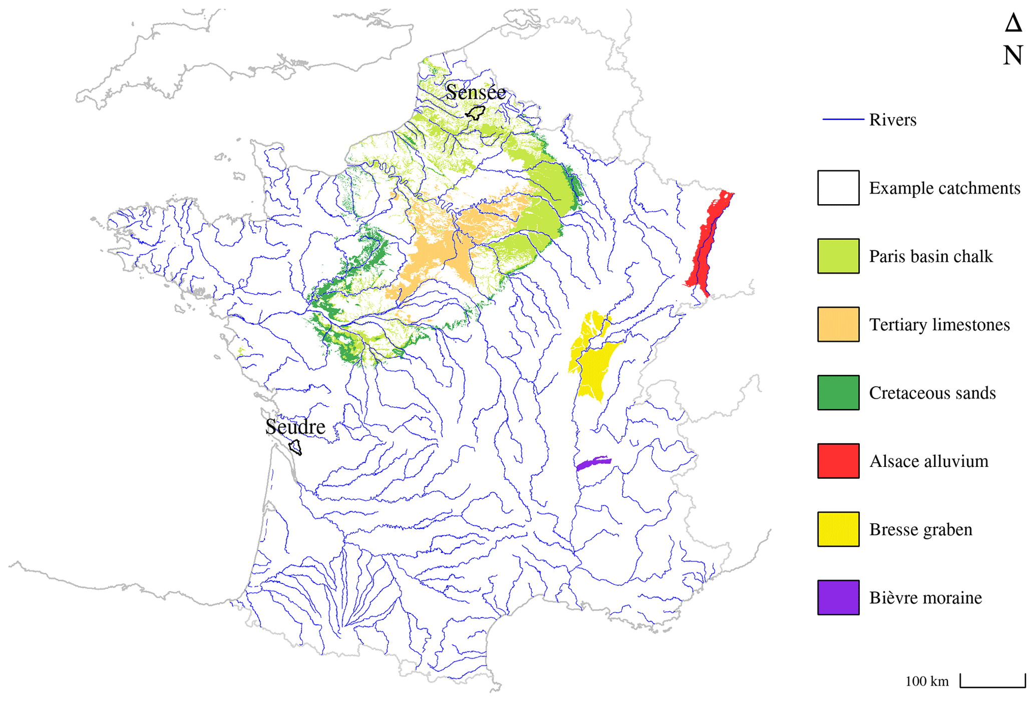
Figure 1 Outcropping areas of several major aquifers in mainland France, and the locations of the example catchments shown in Fig. 2.

The large sedimentary basins are not the only geological areas in France that host aquifers of interest for surface hydrology modelling. Aquifers located in alluvial plains, such as the international Rhineland aquifer – and its French part in the Alsace plain Quaternary alluvium – or the Bresse graben gravels, play a major role in the streamflow dynamics of the Saone and the Rhine basins. As highlighted in the “Introduction”, even small alluvial aquifers outside plains can have an influence on rivers: for example, several small left-bank tributaries of the Rhone are mostly fed by the Bièvre moraine aquifer, with visible consequences for water quality (Bel et al., 1999). Regions in which geological formations are composed of metamorphic or igneous rocks, such as Brittany or the Ardennes, can host fractured bedrock aquifers linked to surface rivers. The wide monitoring network of rivers and groundwater in France, described below, allowed us to select a test dataset of catchments that is representative of this diversity.

2.2 Data sources

Climatic data – daily cumulative precipitation, average temperature and fraction of solid precipitation – were taken from the SAFRAN (Système d'Analyse Fournissant des Renseignements Adaptés à la Nivologie) re-analysis (Vidal et al., 2009) by Météo France; they are available for daily time steps for the 1958–2018 period. Daily potential evaporation was computed using the formula of Oudin et al. (2005). Streamflow data were retrieved from the French national database, Banque Hydro (Leleu et al., 2014; SCHAPI, 2021). These hydroclimatic data are aggregated at the catchment scale and for daily time steps for mainland France in the HydroSafran database (Delaigue et al., 2021) maintained by INRAE (Institut national de recherche pour l'agriculture, l'alimentation et l'environnement).

Groundwater level data are from the French national database ADES, (BRGM, 2021) (Accès aux données sur les eaux souterraines), which gathers piezometric data from many providers in the French territory. Selected piezometers were taken from two reference networks to ensure the quality of data: RNESOUPMOBRGM (the national quantitative monitoring network managed by BRGM, the French national geological survey) and RNESP (the heritage national network for groundwater monitoring).

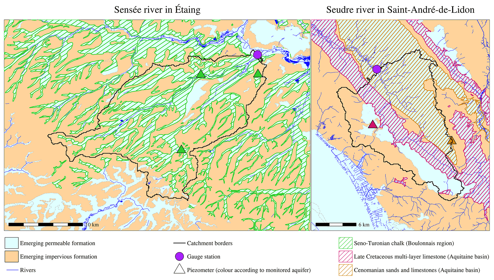
Figure 2 Two examples of hydrogeological maps of catchments used for dataset selection. Their locations in the French mainland territory are shown in Fig. 1.

2.3 Dataset selection

Catchments were selected on the basis of data availability criteria, shown below, and an analysis of the hydrogeological context through the French national reference cartography of hydrogeological formations, BDLISA (Brugeron et al., 2018) (Base de données des limites des systèmes aquifères). For each catchment, one or several piezometers were chosen to assess the connections of the monitored aquifers with surface water bodies. First, using the provided metadata, each piezometer extracted from the ADES database was associated with a hydrogeological entity in BDLISA representing an aquifer. Catchments in which anthropogenic activities – dams, major direct withdrawals or inflows – are known to have a significant influence on streamflow and catchments in which more than 10 % of the precipitation falls as snow were discarded. Then, for each catchment, piezometers associated with aquifers emerging inside the catchment boundaries were listed, and maps – see an example in Fig. 2 – were produced to assess the importance of each hydrogeological formation for the catchment. Piezometers associated with formations with outcropping or sub-outcropping areas representing less than 5 % of the catchment area were discarded, along with those located on the wrong sides of underground watersheds – i.e. where groundwater does not flow to the catchment outlet but to another catchment – as identified by BDLISA.

After this spatial selection, the available groundwater level and streamflow data were examined. An initial visual inspection of the time series was performed to eliminate data for which the quality was too low, relying on the expertise of the database maintainers. Then, catchments and piezometers were selected according to the following criteria:

• at least 20 years of continuously available streamflow data with less than 10 % of the data missing

• at least 20 years of continuously available groundwater level data with less than 10 % of the data missing

• at least 10 years of continuous contemporaneity between streamflow and groundwater level.

Figure 2 shows two situations encountered at this stage: on the left, the Sensée river is connected to one monitored aquifer, but three piezometers are available. In this case, the piezometer with the longest time series with respect to contemporaneity with the streamflow data was selected to represent the aquifer. On the right, the Seudre river is connected to two monitored aquifers, with one piezometer for each; in this case, the two piezometers are kept. The choice of keeping only one piezometer per aquifer in the catchment was made for the sake of simplicity; in most catchments, when visually comparing the dynamics of the groundwater level time series, no major difference was encountered between piezometers monitoring the same aquifer within the same catchment. A correlation study between groundwater level time series led to the same conclusions.

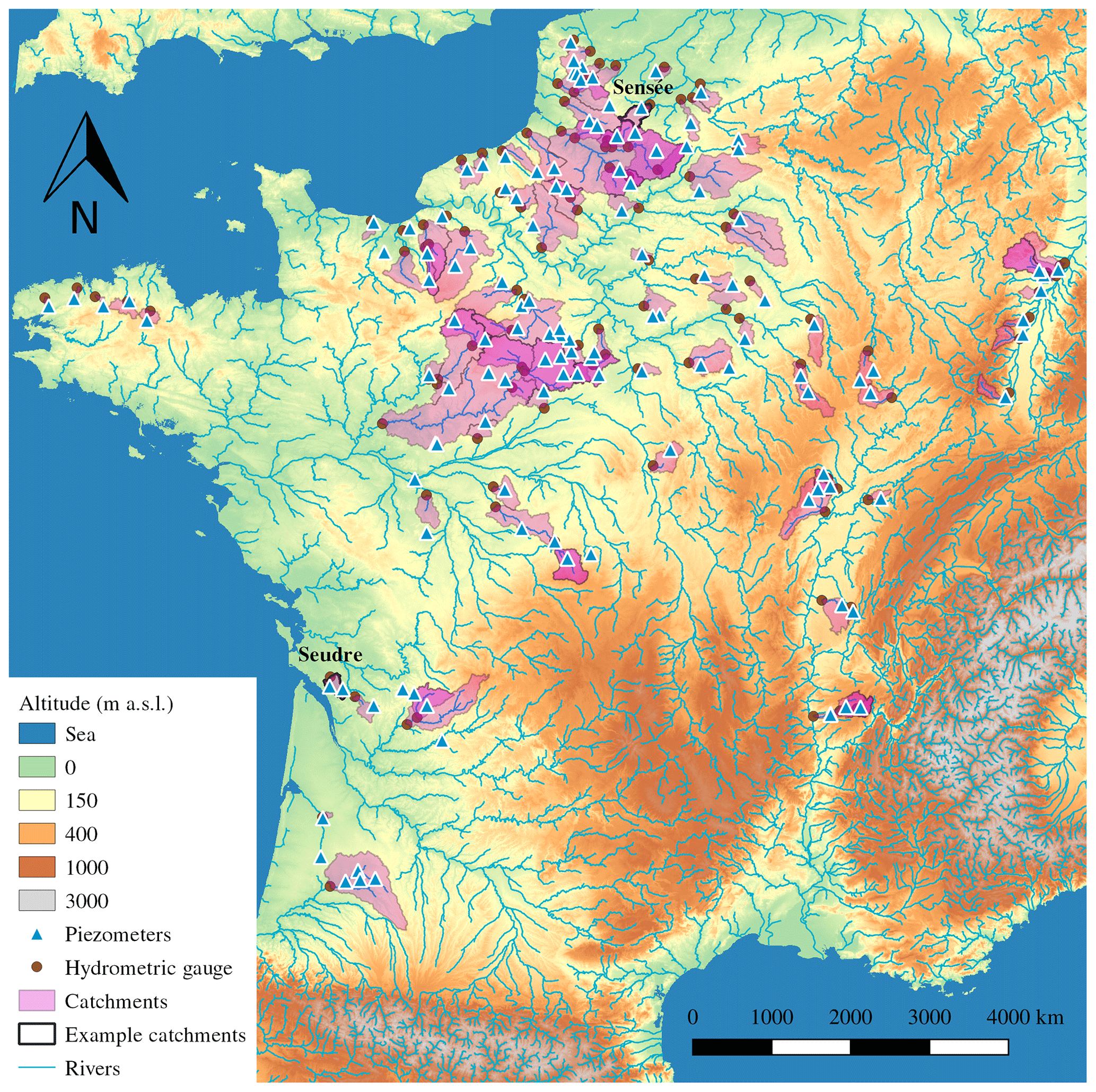
Figure 3 Map of the catchments and the piezometer dataset. The example catchments of Fig. 2 are shown.

Finally, this selection process yielded a set of 107 catchments and 160 piezometer/catchment pairs. The majority of the catchments – 73 – are associated with only 1 piezometer; 22 of them with 2; 8 of them with 3; 1 of them with 4; and 3 of them with 5 piezometers. Tables 1 and 2 show geographical and hydrogeological characteristics of the set. The necessity to choose catchments that are not anthropogenically regulated led to a selection mainly composed of small headwater catchments that are representative of the climatic diversity of the French territory. Dismissing the mountainous catchments to avoid the influence of snow favoured the selection of lowland catchments, although several Vosges catchments whose downstream parts are linked to the Alsace plain aquifer reach maximum altitudes above 1000 m. However, the average altitude remains low enough for the solid precipitation fraction not to overtake 10 % of the total precipitation at the catchment scale. The variability of the mean annual potential evaporation is low, since the dataset does not contain high-altitude catchments – in which low yearly PET values are observed – or catchments located in the south-east of France – where the highest PET values are reached (Brigode et al., 2021).

Table 1 Geographical characteristics of the 107-catchment dataset.

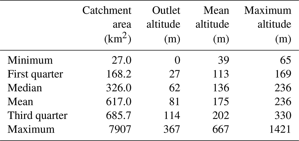
Table 2 Hydrological characteristics of the catchment dataset. The aridity index is defined as the quotient of annual rainfall and annual potential evaporation (PET). Catchment yield is the quotient of annual streamflow and annual rainfall.

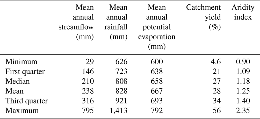
Figure 3 shows a map of the selected catchments and piezometers. The northern part of mainland France, especially the Paris basin, is over-represented because of data availability; in particular, the chalk and Tertiary limestone aquifers in this basin are the hydrogeological formations that have been monitored for the longest time in the territory. However, attention was paid to ensuring that the diversity of hydrogeological contexts was represented through smaller local aquifers or fractured bedrock aquifers, in order to assess the proposed modelling approach in the widest possible range of configurations.

3 Methodology

3.1 Presentation of the original GR6J model

3.1.1 General presentation

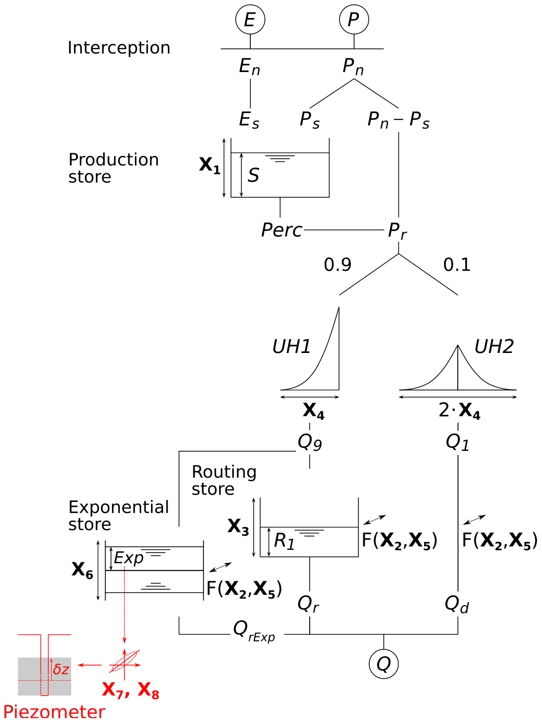
GR6J – which stands for “modèle du Génie Rural à 6 paramètres Journalier” – is a daily six-parameter rainfall–runoff model. It was developed by Pushpalatha et al. (2011) as an evolution of previous GR4J (Perrin et al., 2003) and GR5J (Le Moine, 2008) versions, using a conceptual description of the hydrological processes taking place in the catchment: the model structure, visible in black in Fig. 4, is composed of stores, unit hydrographs and empirical equations that link them. The model is lumped and operates at daily time steps, taking as inputs the precipitation P and potential evaporation E averaged across the time step and the spatial extent of the catchment. GR6J is also parametric, i.e. for each catchment, six independent parameters have to be identified. All variables and parameters are expressed either as the water depth in millimetres or are unitless.

Figure 4 Structure of the original GR6J model – in black – and the built-in piezometry simulation module – in red. See Table C1 in Appendix C for the definitions of the parameters and variables.

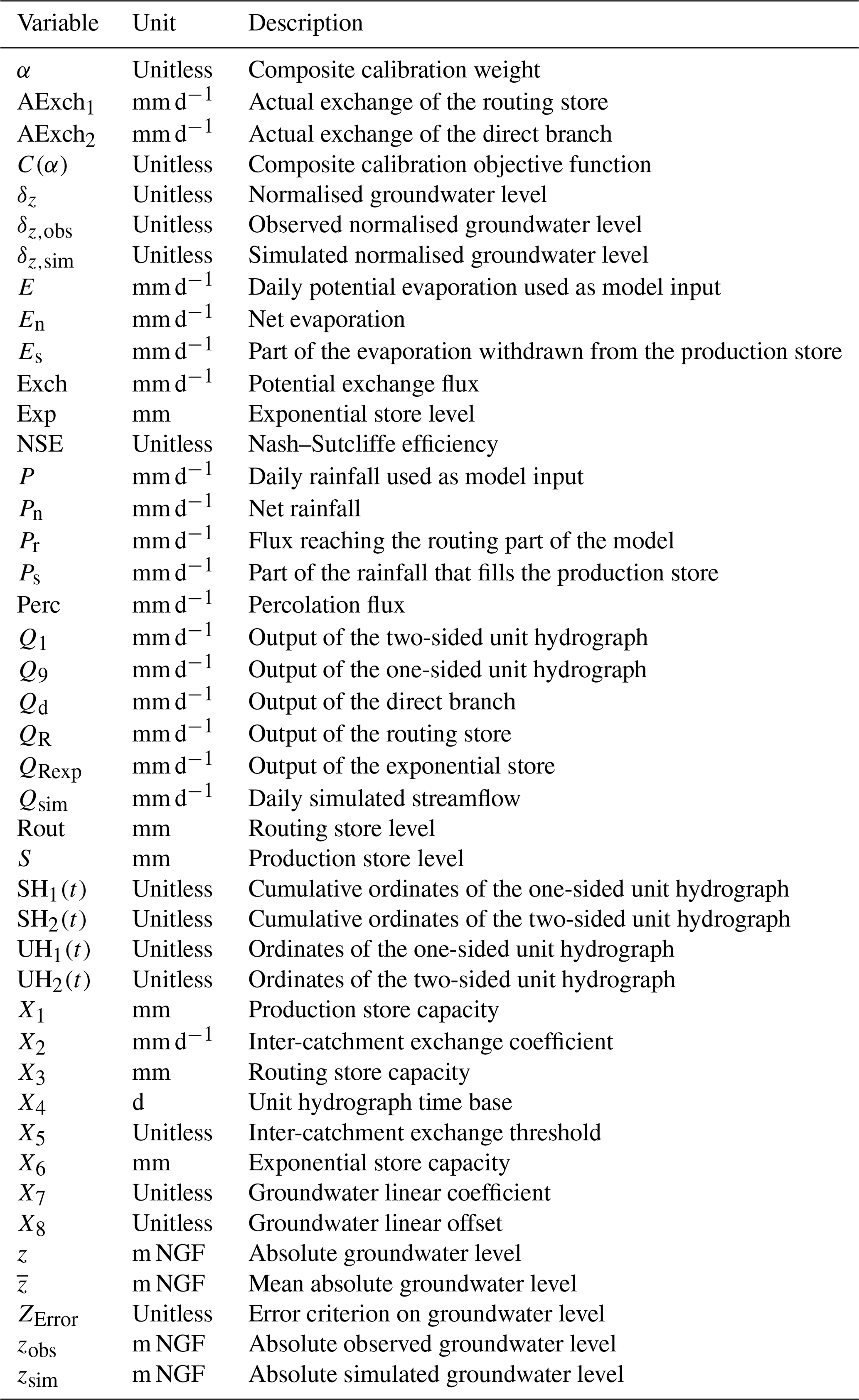
The aim of this section is not to report the modelling tests that have led to the development of the GR6J structure since the original paper by Michel (1983) – such discussions can be found in Perrin et al. (2003), Le Moine (2008) or Pushpalatha et al. (2011). A summary description of the model computations is available in Appendix A; a table of variables is available in Appendix C. Computing codes can be found in the open-source airGR package (Coron et al., 2017, 2021) available in R (Slater et al., 2019; R Core Team, 2021).

3.1.2 Parametrisation strategy

For each catchment, the model is calibrated to fit the measured streamflow: the six parameters are determined through an optimisation process where an error criterion between the measured and simulated streamflows in a reference period is minimized. In this study, the Nash–Sutcliffe efficiency or NSE (Nash and Sutcliffe, 1970) was used for streamflow.

Since the six parameters have very different dimensions and variation ranges, each of them is transformed with a bijective function to fit into the [−9.99; 9.99] interval. Thereby, the optimisation space for optimal parameter research becomes [−9.99; 9.99]⁶, which helps most optimisation algorithms find the global optimum. Detailed transformations and ranges are available in Appendix B. Several optimisation algorithms are used to calibrate the GR6J model; examples can be found in Coron et al. (2021).

3.2 Study of the correlation of the model with piezometry

To adapt the existing model structure for groundwater level simulation, we followed an approach similar to other lumped conceptual models, i.e. a store was used as a representation of the aquifer, and the water content in the store was regarded as a proxy for groundwater level. With this aim in mind, a correlation study was performed on the dataset presented in Sect. 2 in order to identify which of the three conceptual reservoirs of the model structure was the most correlated with piezometry. The production store is part of the production function, which computes the balance between rainfall and evaporation to determine the amount of water available for streamflow. The routing and the exponential stores are part of the routing function, which models the time repartition of this available water to simulate streamflow.

GR6J was calibrated for the 107 catchments of the dataset using the Nash–Sutcliffe efficiency criterion computed on the square root of streamflow. The algorithm of Michel (1991), as implemented in the R package airGR (Coron et al., 2021; R Core Team, 2021), was used for the whole period of available climatic data (1958–2018). Then, the time series of model states obtained – the levels of the three conceptual stores and the simulated streamflow used as control data – and the groundwater level time series were aggregated at monthly time steps to avoid problems caused by missing piezometry measurements. Afterwards, for each of the 160 catchment/piezometer pairs, Spearman's correlation (Spearman, 1907) between piezometry and each state series was computed; the results are summarised as boxplots in Fig. 5. The exponential store (Michel et al., 2003) – see Fig. 4 for a description of the model – is the most strongly correlated with piezometry, and, moreover, it is the only store to be more correlated with groundwater level than with streamflow. The median correlation obtained is 0.762, and 80 % of pairs reach a value higher than 0.5.

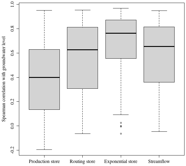
Figure 5 Distributions of the correlations between piezometry and several states of the model.

A high Spearman correlation may highlight a non-linear relationship, since it is a rank correlation. However, this does not seem to be the case here: other investigations not detailed here show that the relationship between the exponential store content and the groundwater level can be regarded as linear – all the more so as the correlation is high. Therefore, it was decided to use the exponential store to simulate piezometry with an adapted scheme presented in the following section.

3.3 Adaptation of the model scheme

A built-in module is added to the existing model structure to simulate groundwater level. The streamflow simulation chain is not modified, but a new output is added to the model through a linear transformation of the exponential store level.

Absolute groundwater level values strongly depend on the piezometer location – its altitude, but also its position with respect to the catchment topography. Indeed, two piezometers monitoring the same aquifer and therefore representing the same dynamics can have different mean levels, and their fluctuations can have different ranges – for instance, if the first one is located on a plateau while the second one is on a slope. To avoid having to take into account these problems, it was decided to work with the normalised groundwater level δz:

$$\begin{array}{}\text{(1)}& \mathit{\delta }z={\displaystyle \frac{z-\stackrel{\mathrm{‾}}{z}}{{\mathit{\sigma }}_z}},\end{array}$$

where z is the absolute groundwater level, $\stackrel{\mathrm{‾}}{z}$ is its mean and σ_z is its standard deviation. To represent the relationship between the exponential store level “Exp” – in mm – and the simulated normalised groundwater level δ_z,sim, several polynomial relationships were investigated. It appeared that using a function of degree 2 or more was not useful for improving performance. Therefore, an affine relationship that includes two additional parameters, X₇ and X₈, is added to the model, using the following equation:

$$\begin{array}{}\text{(2)}& {\mathit{\delta }}_{z,\mathrm{sim}}={\displaystyle \frac{\mathrm{1}}{X_{\mathrm{7}}}}\left({\displaystyle \frac{\mathrm{Exp}}{X_{\mathrm{6}}}}+X_{\mathrm{8}}\right).\end{array}$$

The simulated piezometry z_sim can be computed by reversing Eq. (1):

$$\begin{array}{}\text{(3)}& z_{\mathrm{sim}}={\mathit{\sigma }}_z{\mathit{\delta }}_{z,\mathrm{sim}}+\stackrel{\mathrm{‾}}{z}.\end{array}$$

X₇ is the groundwater linear coefficient; trials have shown that it generally takes values between 0 and 1, but can reach 4. X₈ is called the groundwater linear offset and takes non-negative values, with an upper bound at 20. The new built-in module is shown in red in Fig. 4.

3.4 Composite calibration strategy

Now that two additional parameters have been added to the model structure to simulate piezometry, it is necessary to determine their values through an adapted parametrisation strategy. A composite objective function is chosen for calibration, using a linear combination of a criterion based on streamflow – the Nash–Sutcliffe efficiency computed on the square root of streamflow – and a criterion based on piezometry called Z_Error and defined as

$$\begin{array}{}\text{(4)}& Z_{\mathrm{Error}}=\mathrm{1}-\sum _t{\left({\mathit{\delta }}_{z,\mathrm{sim}}\left(t\right)-{\mathit{\delta }}_{z,\mathrm{obs}}\left(t\right)\right)}^{\mathrm{2}}.\end{array}$$

Computations detailed in Appendix D show that this criterion is in fact the Nash–Sutcliffe efficiency expressed for the groundwater level instead of streamflow. Since the two criteria based on streamflow and piezometry have the same variation ranges, i.e. ]−∞; 1], and the same properties, the objective function C for composite calibration can be taken to be a linear combination of the two criteria with a weight α:

$$\begin{array}{}\text{(5)}& C\left(\mathit{\alpha }\right)=\mathit{\alpha }{Z}_{\mathrm{Error}}+(\mathrm{1}-\mathit{\alpha })\mathrm{NSE}.\end{array}$$

α can take any value between 0 and 1: α=0 means that the calibration is performed only on streamflow and α=1 only on piezometry. In order to find a compromise between these two objectives, 51 values are explored from 0 to 1 in steps of 0.02. For each value of α, C(α) is maximised as a function of eight parameters. The parameter space transformations described in Appendix B are used to convert the optimisation space into the hypercube [−9.99; 9.99]⁸. The differential evolution global optimisation algorithm – implemented in the R package RcppDE (Price et al., 2006; Mullen et al., 2011; Ardia et al., 2011a, b; Eddelbuettel, 2018; Slater et al., 2019; Ardia et al., 2020; R Core Team, 2021) – is then executed to find the global optimal point for the eight parameters.

3.5 Split-sample test evaluation scheme

To assess the effect of the new calibration scheme described above on the streamflow simulation performance, a split-sample test (Klemeš, 1986) is conducted for each catchment/piezometer pair in the assessment dataset described in Sect. 2. For each pair, the available data are divided into two time periods P₁ and P₂ of equal length, defined so as to encompass the same number of data points for which both groundwater level and streamflow are available. Thereby, both periods contain the same amount of information and can be equally used for calibration and validation. The exact duration of the periods depends on the pair, since the time periods with available data have diverse durations, ranging from 5.6 to 28.5 years by period. Before each period, a warm-up timespan of 5 years is set: the model is run on this period, but the resulting simulated values are not used to compute criteria.

After determining these periods, the adapted model structure is calibrated on P₁ using C(α) for each value of α; the parameter set obtained is then used to run the model on P₂ and compute several validation criteria. Then, the periods are switched and the same procedure is executed. The following validation criteria are used:

• $\mathrm{NSE}\left(\sqrt{Q}\right)$, to evaluate the model performance for the whole streamflow spectrum

• $\mathrm{NSE}\left(\sqrt[\mathrm{3}]{Q}\right)$, to evaluate the model performance for low flows; this was preferred rather than zero-diverging transformations such as $\frac{\mathrm{1}}{Q}$ or log (Q) to avoid numerical problems with very low streamflow values

• Z_Error, to assess the model performance in groundwater level simulation.

Since the evaluation is performed for validation, the results presented in Sect. 4 are, unless otherwise specified, validation results.

To assess the benefit of using groundwater level data in the calibration process, the distributions of evaluation criteria values need to be compared to reference ones. For streamflow, the value α=0 corresponds to the original calibration framework performed only on observed streamflow data. Parameters X₇ and X₈ are only used to simulate the normalised groundwater level and therefore, when α=0, the sensitivity of the calibration criterion to their values is zero. Thus, they are randomly determined by the stochastic optimisation algorithm, and no relevant normalised groundwater level is simulated except a random affine transformation of the exponential store level, which cannot be compared to observed data. Therefore, a reference distribution other than the one obtained for α=0 is needed to evaluate groundwater level simulation. The value α=1 is used, since it is the case in which the model is calibrated only with observed groundwater level data and no streamflow; we thus expect the best theoretically possible groundwater level simulation performance for this value of α.

The differences between the evaluation criteria distributions are evaluated visually and then, in order to objectify them, a Wilcoxon–Mann–Whitney test (Wilcoxon, 1945; Mann and Whitney, 1947; Bauer, 1972) is conducted. The distributions obtained for the values of α are compared with the reference ones: α=0 for NSE; α=1 for Z_Error. Therefore, for each value of α, two tests are conducted: one to assess whether the streamflow simulation performance has significantly deteriorated, and one to evaluate whether the performance in groundwater level simulation is significantly lower than the one obtained for α=1.

To assess the influence of the geological context, the test dataset of 160 catchment/piezometer pairs was divided into six groups, as detailed in Table 3. The groups were established in accordance with the hydrogeological formation attributed to each piezometer in the BDLISA reference inventory of Brugeron et al. (2018). This classification may look arbitrary or inaccurate, since each piezometer corresponds to an idiosyncratic local situation; however, such a subgroup analysis of the test dataset highlights the influence of geology on model performance.

Table 3 Groups of catchment/piezometer pairs gathered by geological context.

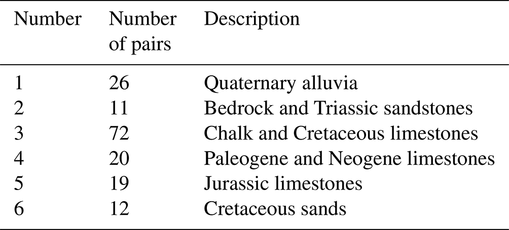
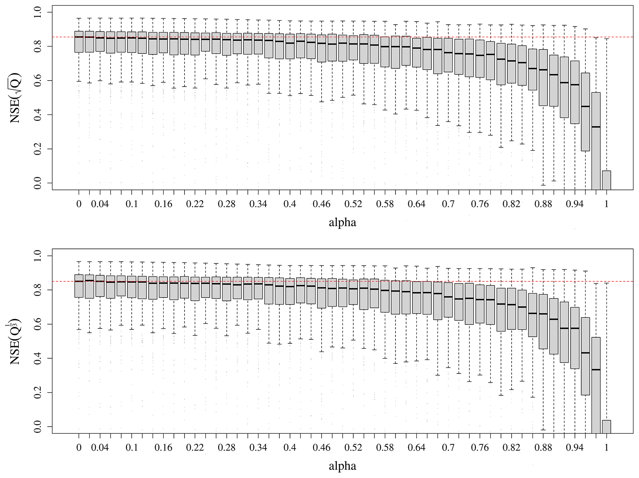
Figure 6 Distributions of the NSE criterion values obtained in validation by the modified model on the 107 catchments for the 51 values of α, the criterion weight. The dashed red line indicates the median NSE value for the original calibration strategy α=0. Values below 0 are cut off for readability.

4 Results and discussion

4.1 Is low-flow simulation improved?

The model performance for streamflow simulation in validation is not improved by the proposed calibration scheme. Figure 6 shows that the distribution of Nash–Sutcliffe efficiency computed on the square root of streamflow does not appear to change significantly for values of α under 0.34; for higher values, the performances deteriorate, but it is surprising to note that they slowly decrease with increasing α, and they remain acceptable until α=0.84 – even though the loss of about 0.2 is significant. Beyond these values, the performances have considerably deteriorated: the calibration cannot be suitably performed on groundwater level time series only; this is an expected result, since the dynamics of the groundwater level and streamflow signal are different. The same trend is observed with the performances for low flows, as assessed through the Nash–Sutcliffe efficiency computed on the cube root of the streamflow.

4.2 Is the model able to simulate groundwater levels?

The model appears to be able to simulate groundwater levels with a satisfactory performance. Figure 7 shows the distributions of the Z_Error criterion for the 51 values of α compared to the theoretical maximum possible performance, which is obtained with α=1, i.e. a calibration performed only on groundwater level with no streamflow information. The distribution of Z_Error values appears to be similar for all α values above 0.34, with a median Z_Error of around 0.70. For α between 0.12 and 0.34, the performance decreases slightly but remains close to the best possible performance, with a median Z_Error of around 0.66. Finally, when α is under 0.1, with very little groundwater level information added to the calibration process, the performance is much lower, but it is acceptable even for α=0.02, with a median Z_Error of around 0.5.

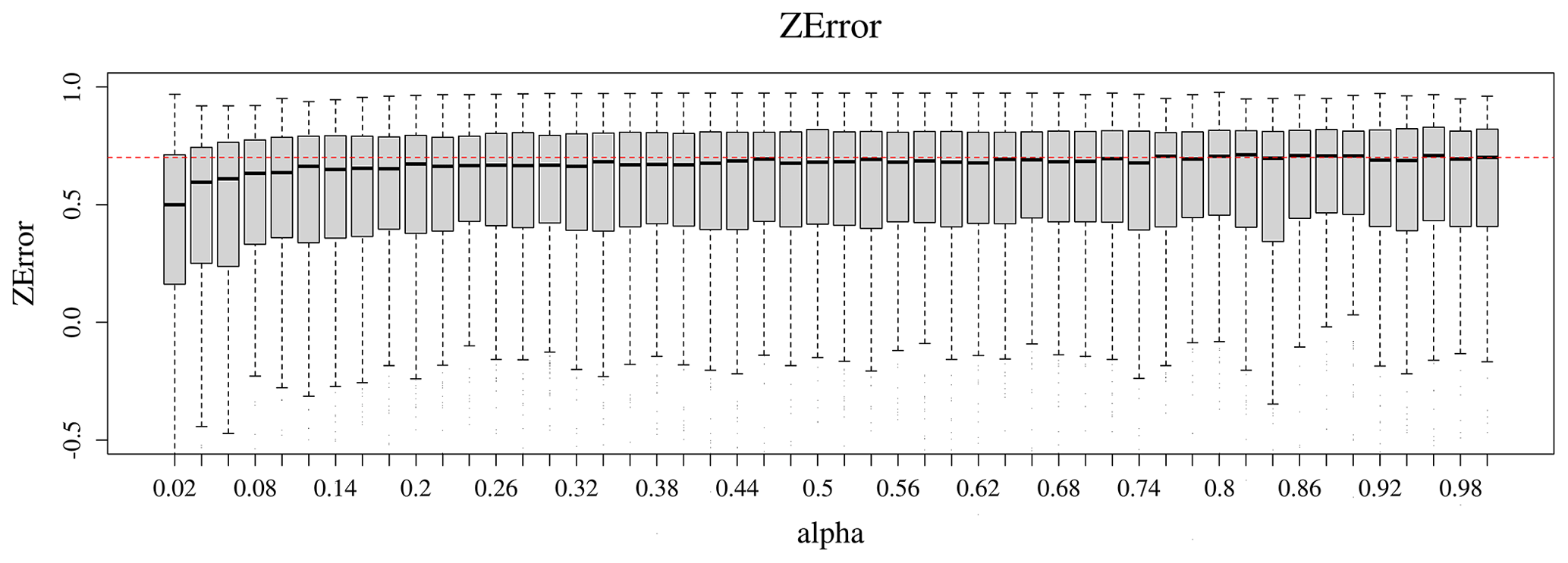
Figure 7 Distributions of the Z_Error criterion values obtained for 50 values of α, the criterion weight. α=0 was discarded since no groundwater level simulation is performed for that case. The dashed red line indicates the median Z_Error value obtained with α=1. Values below −0.5 are cut off for readability.

4.3 Recommended calibration framework and examples

Results of the statistical evaluation of differences between performance criteria distributions are presented as p-values in Fig. 8, with a significance threshold of 5 %.

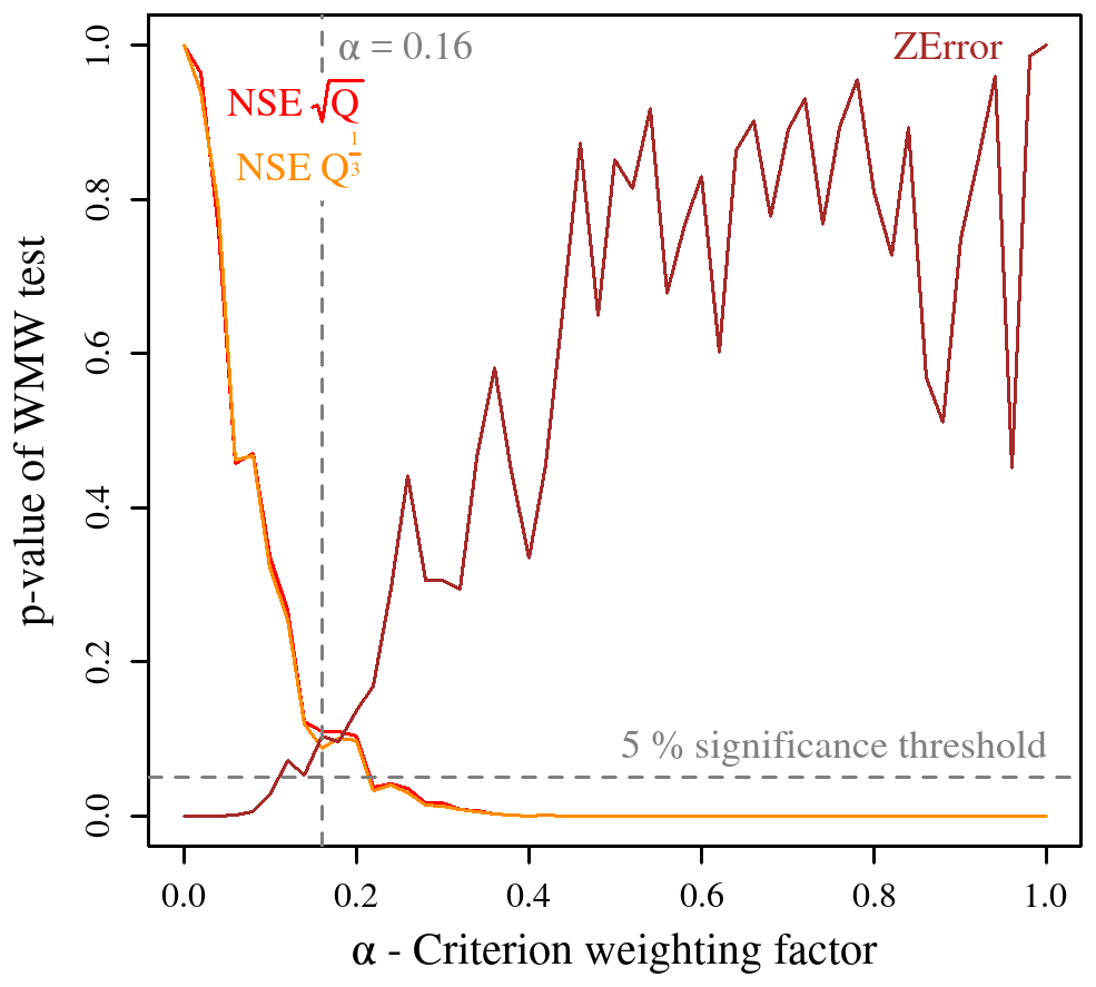
Figure 8 p-values of the Wilcoxon–Mann–Whitney (WMW) tests comparing the criteria value distributions obtained for the 51 values of α with reference ones.

It appears that for values of α greater than 0.22, streamflow simulation performance has significantly deteriorated; for α lower than 0.12, groundwater level simulation performance is significantly below that obtained for higher values of α. A narrow interval, α between 0.14 and 0.2, corresponds to values for which the model performance for both outputs is comparable to reference distributions: the model is as good at streamflow simulation as the original model, and it cannot be better at groundwater level simulation. Therefore, it was decided to choose the value α=0.16 as the recommended calibration framework, even though any value in the described interval could be chosen without significantly changing the results.

Figures 9 and 10 present an example of the application of the new calibration framework to the Sensée catchment in Étaing, in the north of mainland France. The Sensée River is a tributary of the Scheldt (Escaut), which is influenced by the Seno-Turonian chalk aquifer – see Fig. 2. This catchment is an outlier with respect to the model performance distribution, since the Nash–Sutcliffe efficiency is improved by 0.14 for the period shown in the figures. However, this large difference is difficult to visualise, since the two simulated hydrographs are close. The Z_Error obtained is average (0.630), and multi-year groundwater dynamics are reproduced, but the model struggles to simulate the peaks of the observed piezometry time series.

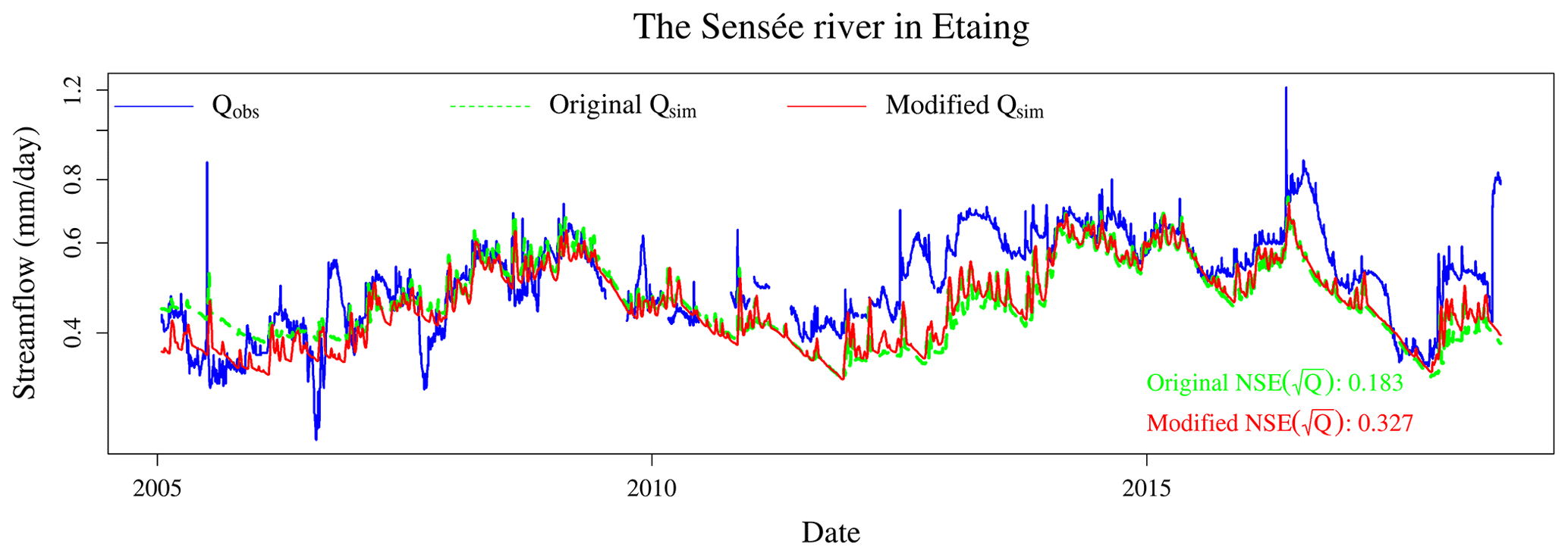
Figure 9 Observed and simulated streamflows of the Sensée River in Étaing, where the simulated streamflow was obtained with the original and the new calibration frameworks. A log scale is used to focus on low flows.

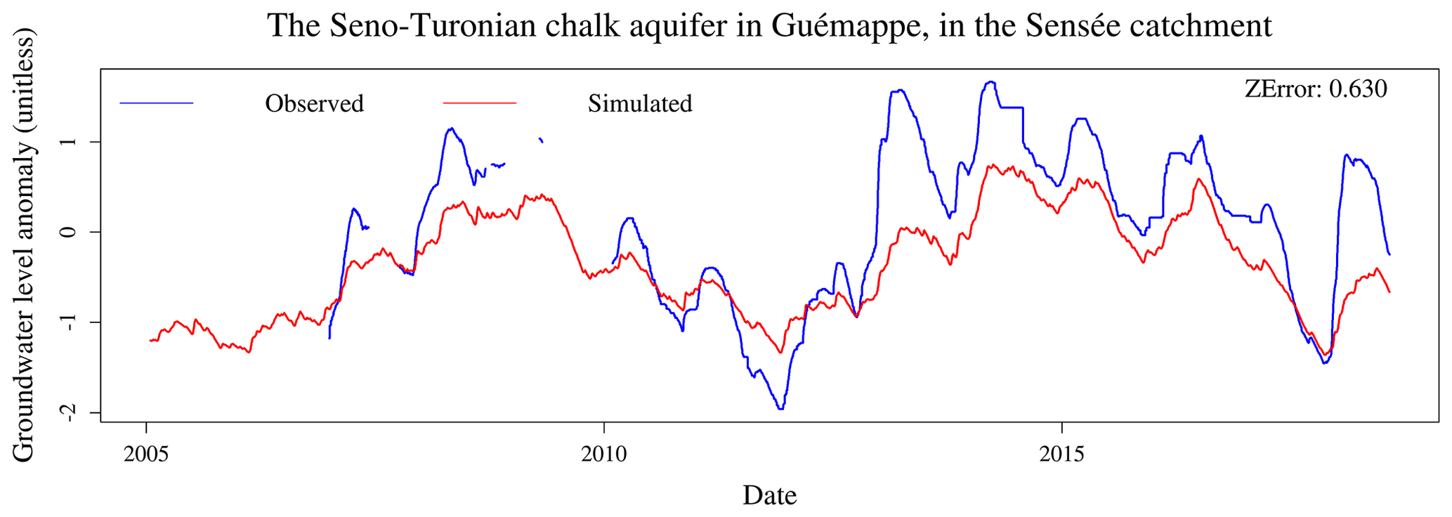
Figure 10 Observed and simulated groundwater levels in the Sensée catchment, where the simulated groundwater level was obtained with the new calibration frameworks.

Figure 11 Observed and simulated streamflows of the Seudre River in Saint-André-de-Lidon, where the simulated streamflow was obtained with the original and the new calibration frameworks. A log scale is used to focus on low flows.

Another example catchment is presented in Figs. 11–13: the Seudre River in Saint-André-de-Lidon. This is a small coastal river located in Saintonge that is linked to two regional aquifers of the Aquitaine basin – see Fig. 2: the Cenomanian sands and limestones and the Late Cretaceous multi-layer limestones, each being monitored by one selected piezometer. Figure 11 shows the results for streamflow: adding piezometry to the calibration process did not significantly improve the performance, and the simulated hydrographs are not distinguishable. However, the results for groundwater simulation shown in Figs. 12 and 13 are satisfactory, with Z_Error values of 0.734 for Cenomanian sands and limestones and 0.787 for Late Cretaceous limestone. In addition, the main failure period for groundwater level simulation – between 2010 and 2012, during which piezometry is underestimated – is also unsatisfactory for streamflow simulation, since the model is unable to reproduce the whole variability of the hydrograph during this period.

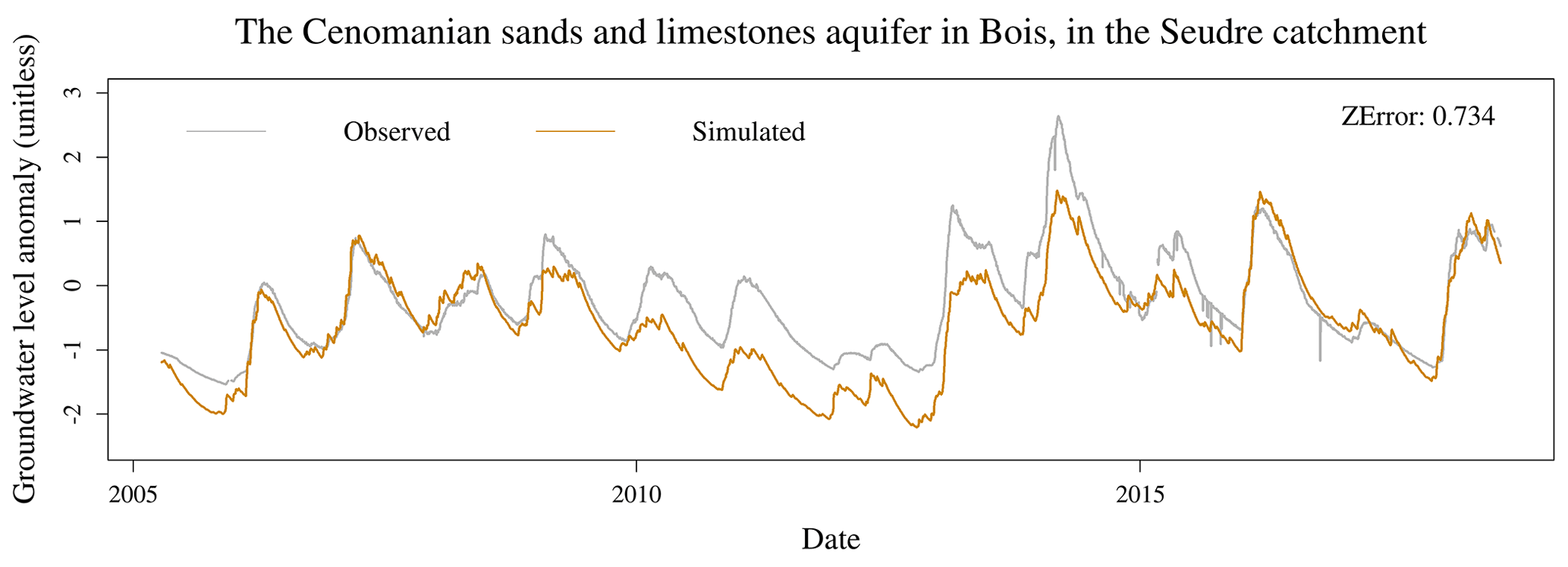
Figure 12 Observed and simulated groundwater levels in the Seudre catchment, where the simulated groundwater level was obtained with the new calibration frameworks: first piezometer.

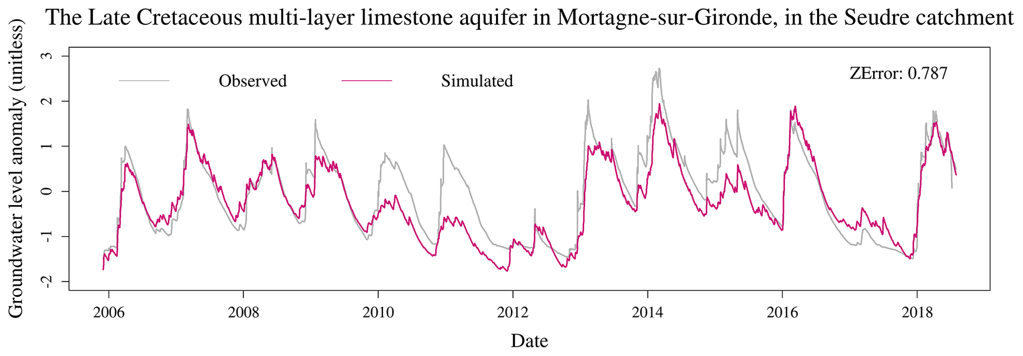
Figure 13 Observed and simulated groundwater levels in the Seudre catchment, where the simulated groundwater level was obtained with the new calibration frameworks: second piezometer.

4.4 Is the new parametrisation stable?

The parametrisation stability between periods is another measure of the robustness of the model: if the parameter values depend on the calibration period, it will cast doubt on the model's capacity to extrapolate streamflow values outside this period and thus to be used, for instance, as a forecasting tool. The split-sample test allows us to assess this stability by comparing the parameter values between the two calibration periods P₁ and P₂. Figure 14 shows the results of this comparison for the six parameters of GR6J and the original calibration framework obtained with α=0; Fig. 15 does so for the modified calibration with the two added parameters. For each parameter, the Pearson correlation between the values obtained for the two periods was computed.

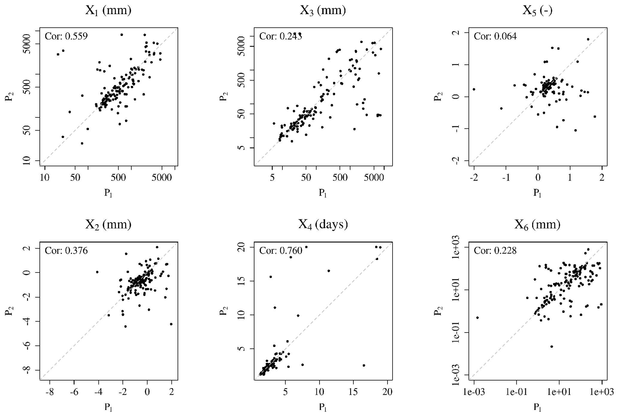
Figure 14 Comparison of the values obtained for the six model parameters through calibration on the two periods of the split-sample test using the original calibration framework with α=0. Log scales are used for visual readability in some plots. The Pearson correlation between periods is indicated.

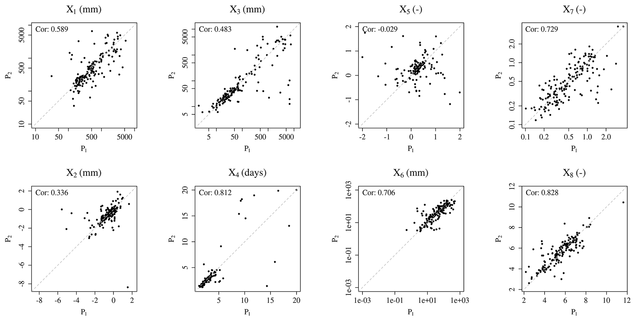
Figure 15 Comparison of the values obtained for the eight model parameters through calibration on the two periods of the split-sample test using the composite calibration framework with α=0.16. Log scales are used for visual readability in some plots. The Pearson correlation between periods is indicated.

The original calibration framework leads to a rather stable parametrisation, except for the exchange threshold X₅, which presents a non-significant correlation between the two periods. The modified calibration using groundwater level data yields more stable parameter values with increased correlations between the two periods, except for the two parameters ruling the inter-catchment exchange function, X₂ and X₅, for which the correlations have slightly deteriorated. The two added parameters, X₇ and X₈, are also very stable between periods, with a correlation of 0.73. Since the modified calibration framework is a new constraint on the routing function, it is not surprising to note that the three routing parameters X₃, X₄ and X₆ become significantly more stable between periods, which is a sign of an improved model robustness.

The difficult transferability of the exchange function parameter values, i.e. the relevance of using them although they were calibrated on another period of time, was highlighted by de Lavenne et al. (2016). This function is sometimes regarded as the flux between catchments, as they are defined by the surface topography, which may not correspond to underground watersheds. Such a situation is common in karstic contexts, see e.g. Le Moine et al. (2008). It can also be considered as a representation of the flux between the catchment and an external aquifer; but in any way, it is merely used by the model as a way to correct the global water budget. Poncelet (2016) underlined the relatively marginal role of the exchange threshold X₅, introduced by Le Moine (2008), in the general performance of the model. The stability issues exposed by the present study highlight the need for further development of this exchange function to take into account the henceforth explicit representation of groundwater level through the exponential reservoir.

4.5 Is performance dependent on the regional and (hydro)geological context?

There is no clear spatial pattern in the results shown in Fig. 16. Since the streamflow simulation performance differences between the original and the composite calibration frameworks are small (and non-significant), the geographical distributions of their performance are similar. High values of performance criteria are noted for the Aquitaine basin, for Brittany, for Upper Champagne and for the downstream tributaries of the Loire River – the Maine and Indre basins. Lower values of NSE are found in the Beauce plain, in the Somme basin, in the inland part of the North region – mostly in the Scheldt (Escaut) basin, and in the Saone and Rhone basin, with the particular case of the Bièvre morainic plain, in which the minimum performance is reached. Other parts of the Paris basin, the North Sea coastal rivers and the Alsace plain have a mixed situation but generally do not reach the extreme points of the NSE distributions.

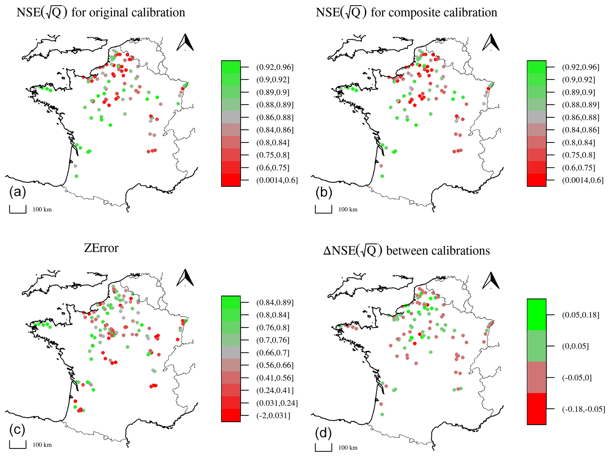
Figure 16 Maps of the results. From (a) to (d): the value of the Nash–Sutcliffe efficiency at each gauge station, computed on the square root of the streamflow, for the original calibration, i.e. α=0; the value of the Nash–Sutcliffe efficiency at each gauge station, computed on the square root of the streamflow, for the composite calibration with α=0.16; the value of the Z_Error criterion at each piezometer for α=0.16; the difference between the NSEs obtained with the composite and the original calibration frameworks. For each point, the maximum value among the catchment/piezometer pairs was chosen.

Catchments in which the performance gain between the two calibration frameworks is significant, i.e. beyond 0.05, are all located either on the Picardy and Normandy chalk or in the Beauce plain. It is interesting to note that this significant improvement is observed in catchments in which the initial model performance was low. However, these areas also host catchments for which the composite calibration framework produces a significant deterioration of streamflow simulation performance.

As for the groundwater level simulation, the performance does not follow the same spatial distribution as the streamflow. High Z_Error values are observed in Brittany and in the western part of the Paris basin, along a crescent running from Artois to Touraine. Lower scores are reached in the Bièvre plain, in Upper Champagne and in the extreme south of Paris basin on the Massif Central piedmont. Other regions have mixed results with no clear spatial pattern.

The sub-group analysis yields clearer results, which are visible in Fig. 17. For the absolute streamflow simulation performance, the original calibration framework yields high values of NSE for groups 2, 4 and 6, medium ones for group 1, and lower scores for groups 3 and 5. These patterns are found again for the composite calibration framework, even though the distribution of performances for group 5 is narrower. Regarding the difference between the two calibration frameworks, a significant improvement for a small part of the dataset is observed in groups 3 and 5 too, with no deterioration of the median performance in the group, while in groups 1, 2, 4 and 6, the median performance is reduced. A significant decrease in performance is observed for a quarter of group 2 and more than a decile of group 4. As for groundwater level simulation, groups 3, 4 and 6 have narrow distributions centred around a high median score of around 0.7, while other groups have much wider distributions, including simultaneously high, medium and low scores.

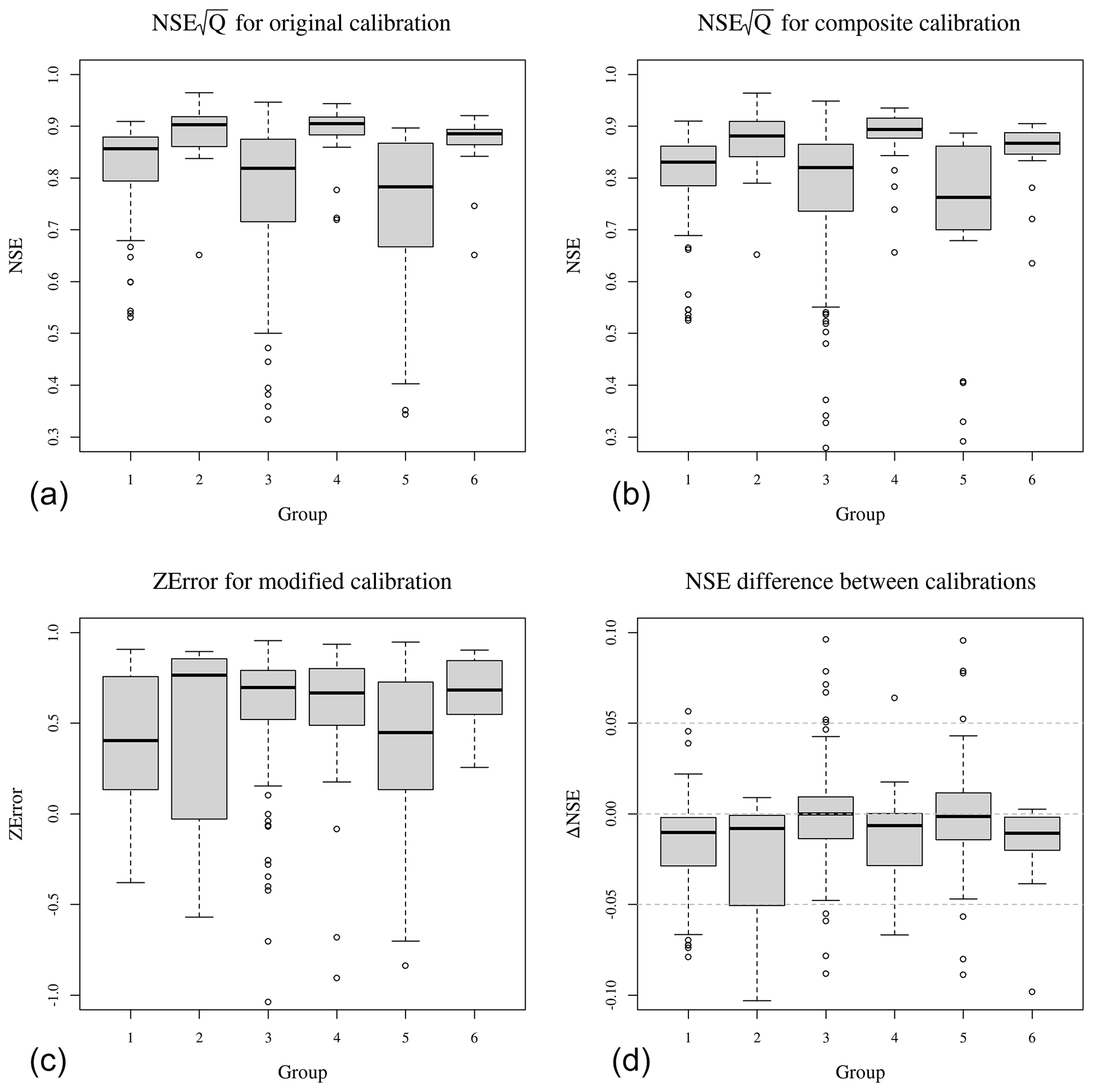
Figure 17 Distributions of the results for groups detailed in Table 3. From (a) to (d): value of the Nash–Sutcliffe efficiency for each pair, computed on the square root of the streamflow, for the original calibration, i.e. α=0; value of the Nash–Sutcliffe efficiency for each pair, computed on the square root of the streamflow, for the composite calibration with α=0.16; value of the Z_Error criterion for each pair for α=0.16; difference in the NSEs obtained with the composite and the original calibration frameworks.

The analysis of the results for groups of catchments with similar hydrogeological contexts allows the formulation of general recommendations to model users, as shown in Sect. 5.2. However, the differences between sub-groups have not been successfully linked to hydrogeological characteristics of aquifers, such as permeability or transmissivity. In fact, these data are difficult to obtain for the French territory, except in experimental, extensively instrumented catchments.

4.6 Are these results model specific? Or dataset specific?

The results presented in the previous sections can be seen as disappointing with reference to the objective of the study. Bringing new information – observed groundwater level data – to the GR6J model yielded no improvement in streamflow simulation performance. Of course, a question arises that we do not wish to avoid in this paper: is this disappointing conclusion model specific, i.e. is it due to the conceptual nature of the GR6J model? Would a less conceptual and more descriptive model have yielded more satisfactory results? Would a more heavily parametrised model have yielded more satisfactory results? Let us first answer this second question: equifinality is a plague in all modelling efforts, and we would not claim as a success an operation that consists of marginally improving the situation of a model that was previously impossible to calibrate. Thus, we reject the critique of model complexity as being unworthy of a modeller. Concerning the physical realism of the model, no a priori conclusion can be drawn about the performance of more physically based models without any empirical evaluation of a large set of catchments. However, the fact that the exponential reservoir – introduced in the GR6J structure to represent slow aquifer transfers – represents the dynamics of piezometers on a large catchment set either well or very well cannot be the consequence of sheer luck. If the piezometric measurements are well represented in both the calibration and the validation period, this means that our mathematical representation is adequate to describe the underlying physical processes, even without it having been designed to do so.

Similar studies performed on other conceptual models did not result in different conclusions: Thiéry (1988) does not mention an improvement in streamflow simulation when calibrating GARDÉNIA with groundwater level data; the study by Moore and Bell (2002) on the PDM model is not conclusive since the new model structure is not compared to a reference one; finally, the calibration framework proposed by Széles et al. (2020) for the HBV model gives a similar conclusion to the one of this study: using groundwater level data for calibration helped to represent aquifer storage in the model but did not improve streamflow simulation.

Regarding the catchment dataset, we tried to use the largest possible set of catchments with respect to our data sources and the selection criteria discussed in Sect. 2.3. A selection bias is possible in the present study, mainly because the aquifers regarded as important for surface water resources are the ones that have been monitored for the longest time at the largest number of measurement points: the chalk aquifer in Picardy and the Alsace plain alluvium of the Beauce Tertiary limestones. However, the catchment dataset used in this study is diverse enough to draw general conclusions, at least for climatic and hydrogeological conditions similar to the ones observed in mainland France. Further evaluation for different contexts in other countries would help to put our results into perspective.

5 Conclusions

5.1 Synthesis

The study presented here concerns the implementation of a new calibration procedure for an existing streamflow simulation model, GR6J; it is not about the development of a completely new model. For each catchment, among all the parameter sets that yield equivalent streamflow simulations, we identified a particular parameter set that is able to additionally simulate groundwater level. This new modelling capacity does not induce a significant deterioration in the streamflow simulation performance; neither does it improve it, except in a few particular cases. However, an advantage of the composite calibration framework was highlighted: since we identified a particular parameter set among equivalent sets for streamflow, we probably reduced equifinality in the model calibration, which is suggested by the parameter stability improvement. We may thus expect a more robust model, even if a specific equifinality study would help enforce this conclusion.

The results presented in this paper can be seen as truly encouraging – a realistic representation of the piezometric variability was obtained as one of the states of the model, but scientific honesty requires us to mention that, to us, they were – at least initially – truly disappointing, because we aimed at improving the overall representation of streamflow through the inclusion of piezometric information, and not the other way around.

5.2 Recommendations to users: which calibration should be used in which context?

The analyses performed in this study lead to the following recommendations for GR6J model calibration:

• In most catchments, no improvement in streamflow simulation would be expected when using a composite calibration framework with groundwater level data.

• In catchments in which the original model already performs well, adding groundwater level data to the calibration is probably useless as a method of improving streamflow simulation performance.

• In catchments in which the model reaches lower validation scores, a performance improvement is possible but not probable, and is most likely to happen in a chalk or Tertiary limestone context.

• The model with composite calibration is able to simulate the groundwater level with satisfactory performance for chalk, Tertiary limestones and Cretaceous sand aquifers.

• Groundwater level simulation is more uncertain for other geological contexts (Quaternary formations, bedrock, Triassic sandstones or Jurassic limestones). Good results have been observed for the bedrock context of Brittany.

5.3 Perspectives

Beyond streamflow simulation, being able to simulate the groundwater level using such a lumped conceptual model – which is much simpler and lighter to implement than usual groundwater models – is likely to lead to new uses of GR6J. Thereby, since GR6J is part of the operational low-flow forecasting platform Premhyce (Nicolle et al., 2020; Tilmant et al., 2020), it is conceivable to use it as a groundwater level sub-seasonal forecasting tool for some chosen points in France, which is crucial for the anticipative management of groundwater resources. Further studies are needed to evaluate the framework in forecasting mode; a data assimilation process may be necessary to improve the forecast liability and smoothness. Although this study does not include any modification of the streamflow simulation scheme, it offers an overview of possible modifications: the division coefficient between the routing and the exponential stores remained fixed in the present study and may become a new model parameter that controls the size of the aquifer–river flux; the role of the exchange function needs to be clarified and its formulation has to become more stable and readable.

Appendix A: Detailed operation of the GR6J model

A1 Production function

The production function is mainly composed of a production store, whose capacity X₁ is the first parameter of the model. Inputs are P, the daily rainfall depth, and E, the daily potential evaporation. Rainfall is neutralised by evaporation to compute the net rainfall P_n and net evaporation E_n through a case disjunction:

• If P>E, then $P_{\mathrm{n}}=P-E$ and E_n=0.

• Otherwise, P_n=0 and $E_{\mathrm{n}}=E-P$.

If P_n is positive, a part of it, P_s, feeds the production store, which has a level S and a parameter X₁:

$$\begin{array}{}\text{(A1)}& P_{\mathrm{s}}={\displaystyle \frac{X_{\mathrm{1}}\left(\mathrm{1}-{\left(\frac{S}{X_{\mathrm{1}}}\right)}^{\mathrm{2}}\right)\tanh \left(\frac{P_{\mathrm{n}}}{X_{\mathrm{1}}}\right)}{\mathrm{1}+\frac{S}{X_{\mathrm{1}}}\tanh \left(\frac{P_{\mathrm{n}}}{X_{\mathrm{1}}}\right)}};E_{\mathrm{s}}=\mathrm{0}.\end{array}$$

Otherwise, a part (E_s) of E_n is taken from the production store:

$$\begin{array}{}\text{(A2)}& E_{\mathrm{s}}={\displaystyle \frac{S\left(\mathrm{2}-\frac{S}{X_{\mathrm{1}}}\right)\tanh \left(\frac{E_{\mathrm{n}}}{X_{\mathrm{1}}}\right)}{\mathrm{1}+\left(\mathrm{1}-\frac{S}{X_{\mathrm{1}}}\right)\tanh \left(\frac{E_{\mathrm{n}}}{X_{\mathrm{1}}}\right)}};P_{\mathrm{s}}=\mathrm{0}.\end{array}$$

The content of the production store is then updated by $S=S-E_{\mathrm{s}}+P_{\mathrm{s}}$. Part (“Perc”) of the water content of the production store percolates to the routing function:

$$\begin{array}{}\text{(A3)}& \mathrm{Perc}=S\left(\mathrm{1}-{\left(\mathrm{1}+{\left({\displaystyle \frac{\mathrm{4}S}{\mathrm{9}{X}_{\mathrm{1}}}}\right)}^{\mathrm{4}}\right)}^{-\frac{\mathrm{1}}{\mathrm{4}}}\right).\end{array}$$

The content of the production store is updated again by $S=S-\mathrm{Perc}$. Finally, the quantity of water P_r that reaches the routing part of the model is $P_{\mathrm{r}}=\mathrm{Perc}+P_{\mathrm{n}}-P_{\mathrm{s}}$.

A2 Unit hydrographs

P_r is divided into two components: 90 % is routed through the one-sided unit hydrograph UH₁ and the remaining 10 % is routed through a two-sided unit hydrograph UH₂. The cumulated ordinates of the unit hydrographs SH₁(t) and SH₂(t) are determined by the basetime X₄ for t∈ℕ:

$$\begin{array}{}\text{(A4)}& {\mathrm{SH}}_{\mathrm{1}}\left(t\right)=\left\{\begin{array}{ll}\mathrm{0}& \mathrm{if}t=\mathrm{0}\\ {\left(\frac{t}{X_{\mathrm{4}}}\right)}^{\frac{\mathrm{5}}{\mathrm{2}}}& \mathrm{if}\mathrm{0}<t<X_{\mathrm{4}}\\ \mathrm{1}& \mathrm{if}t\ge X_{\mathrm{4}}\end{array}\right.\end{array}$$

$$\begin{array}{}\text{(A5)}& {\mathrm{SH}}_{\mathrm{2}}\left(t\right)=\left\{\begin{array}{ll}\mathrm{0}& \mathrm{if}t=\mathrm{0}\\ \frac{\mathrm{1}}{\mathrm{2}}{\left(\frac{t}{X_{\mathrm{4}}}\right)}^{\frac{\mathrm{5}}{\mathrm{2}}}& \mathrm{if}\mathrm{0}<t<X_{\mathrm{4}}\\ \mathrm{1}-\frac{\mathrm{1}}{\mathrm{2}}{\left(\mathrm{2}-\frac{t}{X_{\mathrm{4}}}\right)}^{\frac{\mathrm{5}}{\mathrm{2}}}& \mathrm{if}{X}_{\mathrm{4}}\le t<\mathrm{2}{X}_{\mathrm{4}}\\ \mathrm{1}& \mathrm{if}t\ge \mathrm{2}{X}_{\mathrm{4}}.\end{array}\right.\end{array}$$

Ordinates UH₁(t) and UH₂(t) are then computed by differentiating the cumulated ordinates:

$$\begin{array}{}\text{(A6)}& \begin{array}{rl}{\mathrm{UH}}_{\mathrm{1}}\left(t\right)& ={\mathrm{SH}}_{\mathrm{1}}\left(t\right)-{\mathrm{SH}}_{\mathrm{1}}(t-\mathrm{1});{\mathrm{UH}}_{\mathrm{2}}\left(t\right)\\ & ={\mathrm{SH}}_{\mathrm{2}}\left(t\right)-{\mathrm{SH}}_{\mathrm{2}}(t-\mathrm{1}).\end{array}\end{array}$$

Finally, the respective outputs of the first unit hydrograph (Q₉) and the second one (Q₁) are computed through a convolution of P_r:

$$\begin{array}{}\text{(A7)}& {\displaystyle }& {\displaystyle }{Q}_{\mathrm{9}}\left(t\right)=\mathrm{0.9}\sum _{k=\mathrm{1}}^{\lfloor X_{\mathrm{4}}\rfloor +\mathrm{1}}{\mathrm{UH}}_{\mathrm{1}}\left(k\right)P_{\mathrm{r}}(t-k+\mathrm{1})\text{(A8)}& {\displaystyle }& {\displaystyle }{Q}_{\mathrm{1}}\left(t\right)=\mathrm{0.1}\sum _{k=\mathrm{1}}^{\lfloor \mathrm{2}{X}_{\mathrm{4}}\rfloor +\mathrm{1}}{\mathrm{UH}}_{\mathrm{2}}\left(k\right)P_{\mathrm{r}}(t-k+\mathrm{1}).\end{array}$$

A3 Routing stores

This part of the model structure is composed of two branches, that of the stores – fed by Q₉ from the first unit hydrograph – and the direct branch – fed by Q₁ from the second unit hydrograph. In the stores branch, Q₉ is partitioned between the two stores, with 60 % for the routing store and 40 % for the exponential store. A potential exchange “Exch” is computed from the water content of the routing store “Rout”, its capacity X₃, and the exchange parameters X₂ and X₅:

$$\begin{array}{}\text{(A9)}& \mathrm{Exch}=X_{\mathrm{2}}\left({\displaystyle \frac{\mathrm{Rout}}{X_{\mathrm{3}}}}-X_{\mathrm{5}}\right).\end{array}$$

This flux can be negative, zero or positive. Since the routing store cannot have a water content (“Rout”) of below zero, the actual exchange flux from the routing store AExch₁ is limited by the content of the latter, which gives the following equation:

$$\begin{array}{}\text{(A10)}& \begin{array}{rl}& {\mathrm{AExch}}_{\mathrm{1}}=\\ & \left\{\begin{array}{ll}\mathrm{Exch}& \mathrm{if}\mathrm{Rout}+\mathrm{0.6}{Q}_{\mathrm{9}}+\mathrm{Exch}\ge \mathrm{0}\\ -\mathrm{Rout}-\mathrm{0.6}{Q}_{\mathrm{9}}& \mathrm{otherwise}.\end{array}\right.\end{array}\end{array}$$

The routing reservoir is then filled with

$$\begin{array}{}\text{(A11)}& \mathrm{Rout}=\mathrm{Rout}+Q_{\mathrm{9}}+{\mathrm{AExch}}_{\mathrm{1}},\end{array}$$

and the output Q_R of the routing reservoir is computed as

$$\begin{array}{}\text{(A12)}& Q_{\mathrm{R}}=\mathrm{Rout}\left(\mathrm{1}-{\left(\mathrm{1}+{\left({\displaystyle \frac{\mathrm{Rout}}{X_{\mathrm{3}}}}\right)}^{\mathrm{4}}\right)}^{-\frac{\mathrm{1}}{\mathrm{4}}}\right).\end{array}$$

The water content of the reservoir is finally updated as $\mathrm{Rout}=\mathrm{Rout}-Q_{\mathrm{R}}$.

As for the exponential store, it is a bottomless reservoir whose water content “Exp” can be negative. Therefore, no case disjunction is necessary, and the store can be filled with

$$\begin{array}{}\text{(A13)}& \mathrm{Exp}=\mathrm{Exp}+\mathrm{0.4}{Q}_{\mathrm{9}}+\mathrm{Exch}.\end{array}$$

Its output is computed as follows, using its capacity X₆:

$$\begin{array}{}\text{(A14)}& Q_{\mathrm{Rexp}}=X_{\mathrm{6}}\log \left(\mathrm{1}+\exp \left({\displaystyle \frac{\mathrm{Exp}}{X_{\mathrm{6}}}}\right)\right).\end{array}$$

The exponential store can now be updated using $\mathrm{Exp}=\mathrm{Exp}-Q_{\mathrm{Rexp}}$.

The second branch, fed by Q₁, is also subject to an exchange AExch₂ with a case disjunction:

$$\begin{array}{}\text{(A15)}& {\mathrm{AExch}}_{\mathrm{2}}=\left\{\begin{array}{ll}\mathrm{Exch}& \mathrm{if}{Q}_{\mathrm{1}}+\mathrm{Exch}\ge \mathrm{0}\\ -Q_{\mathrm{1}}& \mathrm{otherwise}.\end{array}\right.\end{array}$$

The output of the second branch Q_d can now be computed using $Q_{\mathrm{d}}=Q_{\mathrm{1}}-{\mathrm{AExch}}_{\mathrm{2}}$. The simulated streamflow Q_sim is finally computed by adding the components from the three branches:

$$\begin{array}{}\text{(A16)}& Q_{\mathrm{sim}}=Q_{\mathrm{R}}+Q_{\mathrm{Rexp}}+Q_{\mathrm{d}}.\end{array}$$

Appendix B: Parameter ranges and transformations used for original and modified GR6J calibrations

Table B1 Parameter ranges and transformation functions for GR6J model calibration. To make calibration easier, the original parameter search ranges presented below are transformed to [−9.99, 9.99] by each transformation function. The values found are then re-transformed into parameter values using reciprocal transformation. Details can be found in Sect. 3.1.2.

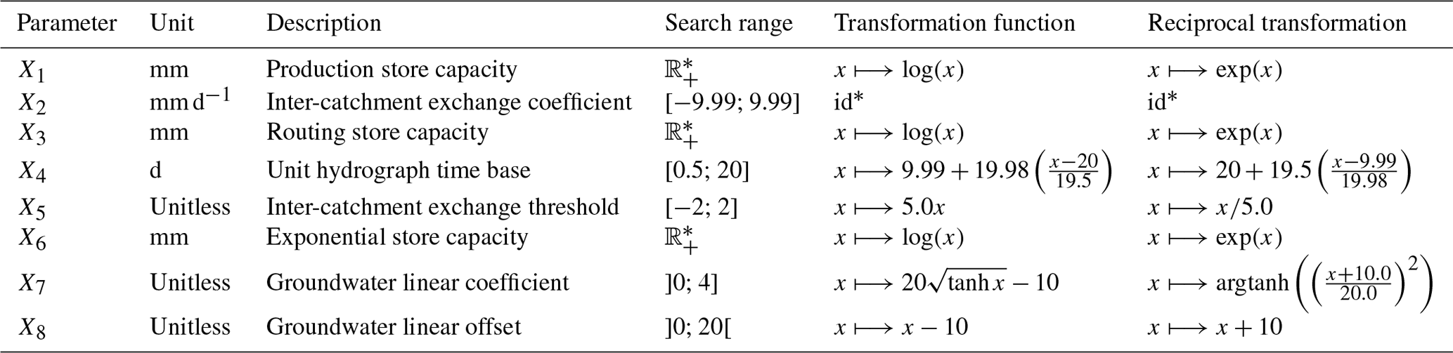
^* id stands for identity function.

Appendix C: Table of variables

Table C1 Table of variables used in the document.

Appendix D: Equivalence between Z_Error and the Nash–Sutcliffe efficiency

The model structure proposed here does not simulate the absolute groundwater level, only its normalised version. Then, by reversing the normalisation equation (Eq. 1), Eq. (3) allows us to get the absolute groundwater level. By combining Eqs. (1), (3) and (4), the following expression for Z_Error is found:

$$\begin{array}{}\text{(D1)}& Z_{\mathrm{Error}}=\mathrm{1}-\sum _t{\left({\displaystyle \frac{z_{\mathrm{sim}}-\stackrel{\mathrm{‾}}{z}}{{\mathit{\sigma }}_z}}-{\displaystyle \frac{z_{\mathrm{obs}}-\stackrel{\mathrm{‾}}{z}}{{\mathit{\sigma }}_z}}\right)}^{\mathrm{2}},\end{array}$$

which gives

$$\begin{array}{}\text{(D2)}& Z_{\mathrm{Error}}=\mathrm{1}-{\displaystyle \frac{\sum _t{\left(z_{\mathrm{sim}}-z_{\mathrm{obs}}\right)}^{\mathrm{2}}}{{\mathit{\sigma }}_z^{\mathrm{2}}}}.\end{array}$$

Based on the definition of the standard deviation, we have:

$$\begin{array}{}\text{(D3)}& {\mathit{\sigma }}_z^{\mathrm{2}}=\sum _t{\left(z_{\mathrm{obs}}-\stackrel{\mathrm{‾}}{z}\right)}^{\mathrm{2}}.\end{array}$$

By combining the two previous equations, we get:

$$\begin{array}{}\text{(D4)}& Z_{\mathrm{Error}}=\mathrm{1}-{\displaystyle \frac{\sum _t{\left(z_{\mathrm{sim}}-z_{\mathrm{obs}}\right)}^{\mathrm{2}}}{\sum _t{\left(z_{\mathrm{obs}}-\stackrel{\mathrm{‾}}{z}\right)}^{\mathrm{2}}}},\end{array}$$

which is exactly the definition of the Nash–Sutcliffe efficiency or NSE (Nash and Sutcliffe, 1970) expressed for groundwater level instead of streamflow. This shows the correspondence between Z_Error and NSE.