the Creative Commons Attribution 4.0 License.
the Creative Commons Attribution 4.0 License.
 | 17 May 2022
Regional, multi-decadal analysis on the Loire River basin reveals that stream temperature increases faster than air temperature
Hanieh Seyedhashemi
Jean-Philippe Vidal
Jacob S. Diamond
Dominique Thiéry
Céline Monteil
Frédéric Hendrickx
Anthony Maire
Florentina Moatar
Stream temperature appears to be increasing globally, but its rate remains poorly constrained due to a paucity of long-term data and difficulty in parsing effects of hydroclimate and landscape variability. Here, we address these issues using the physically based thermal model T-NET (Temperature-NETwork) coupled with the EROS semi-distributed hydrological model to reconstruct past daily stream temperature and streamflow at the scale of the entire Loire River basin in France (105 km2 with 52 278 reaches).
Stream temperature increased for almost all reaches in all seasons (mean ∘C decade−1) over the 1963–2019 period. Increases were greatest in spring and summer, with a median increase of + 0.38 ∘C (range to +0.76 ∘C) and +0.44 ∘C (+0.08 to +1.02 ∘C) per decade, respectively. Rates of stream temperature increases were greater than for air temperature across seasons for the majority of reaches. Spring and summer increases were typically greatest in the southern part of the Loire basin (up to +1 ∘C decade−1) and in the largest rivers (Strahler order ≥5). Importantly, air temperature and streamflow could exert a joint influence on stream temperature trends, where the greatest stream temperature increases were accompanied by similar trends in air temperature (up to +0.71 ∘C decade−1) and the greatest decreases in streamflow (up to −16 % decade−1). Indeed, for the majority of reaches, positive stream temperature anomalies exhibited synchrony with positive anomalies in air temperature and negative anomalies in streamflow, highlighting the dual control exerted by these hydroclimatic drivers. Moreover, spring and summer stream temperature, air temperature, and streamflow time series exhibited common change points occurring in the late 1980s, suggesting a temporal coherence between changes in the hydroclimatic drivers and a rapid stream temperature response. Critically, riparian vegetation shading mitigated stream temperature increases by up to 0.16 ∘C decade−1 in smaller streams (i.e. < 30 km from the source). Our results provide strong support for basin-wide increases in stream temperature due to joint effects of rising air temperature and reduced streamflow. We suggest that some of these climate change-induced effects can be mitigated through the restoration and maintenance of riparian forests.
- Article
(5373 KB) - Full-text XML
-
Supplement
(1933 KB) - BibTeX
- EndNote


Stream temperature is a critical water quality parameter affecting the distribution of aquatic communities (Poole and Berman, 2001; Ducharne, 2008), but its future under global change remains uncertain. As air temperature (Ta) increases worldwide due to climate change, stream temperature (Tw) is expected to follow a similar trajectory (Mohseni et al., 1999; Kaushal et al., 2010; Van Vliet et al., 2011; Isaak et al., 2012; Arora et al., 2016). Indeed, there is growing evidence that stream warming is occurring around the world, affecting freshwater ecosystems through structural and functional changes in biological communities throughout the food web (Woodward et al., 2010; O'Gorman et al., 2012; Scheffers et al., 2016). Deleterious warming effects are documented from bottom-dwelling microorganisms (e.g. Romaní et al., 2016; Majdi et al., 2020) up to macroinvertebrates (e.g. Floury et al., 2013; Bruno et al., 2019) and fish communities (e.g. Maire et al., 2019; Stefani et al., 2020). However, the paucity of long-term time series of Tw (Webb and Walling, 1996; Nelson and Palmer, 2007; Webb et al., 2008; Arora et al., 2016) has impaired the larger-scale assessment of such trends, especially in light of confounding factors like hydrological changes and land-use change. Hence, analyses of Tw trends, especially at large spatiotemporal scales, remain scarce (but see Kaushal et al., 2010; Orr et al., 2015; Arora et al., 2016; Michel et al., 2020; Wilby and Johnson, 2020).
To overcome the lack of Tw data, large-scale ecological studies typically use Ta as a proxy for Tw to assess the impact of climate change on the spatial distribution of aquatic organisms (e.g. Buisson et al., 2008; Buisson and Grenouillet, 2009; Tisseuil et al., 2012; Domisch et al., 2013), but Ta can overpredict changes to stream fish assemblages with climate warming compared with Tw (Kirk and Rahel, 2022). Indeed, Ta can be an imprecise surrogate for Tw (Caissie, 2006), since many landscape and basin characteristics (e.g. stream discharge (Q), streambed morphology, karst resurgences, topography, and vegetation cover) contribute to the response of Tw to climate change over time and space (Stefan and Preud'homme, 1993; Webb and Walling, 1996; Webb et al., 2008; Hannah and Garner, 2015). For instance, riparian vegetation can obstruct solar radiation, which is the dominant heat flux at the air–water surface (Hannah et al., 2004; Caissie, 2006), and therefore decrease Tw response to Ta (Johnson, 2004; Loicq et al., 2018). However, while riparian vegetation shading can greatly decrease the temperature of small rivers (Dan Moore et al., 2005; Loicq et al., 2018), it has limited effects on larger rivers since the width of such rivers is large enough that only a small part of it can be shaded. Rising groundwater temperature (Taylor and Stefan, 2009; Kurylyk et al., 2013, 2014) and reduced groundwater flows (Kurylyk et al., 2014) due to climate change may further contribute to Tw trends (Meisner, 1990; Arora et al., 2016), leading to asymmetric controls (vis-à-vis Ta) on Tw (Moatar and Gailhard, 2006), especially in headwaters (Caissie, 2006; Kelleher et al., 2012; Mayer, 2012). Finally, intensification of the water cycle (Huntington, 2006), with more frequent and severe droughts (Mantua et al., 2010; Giuntoli et al., 2013; Prudhomme et al., 2014), as well as more intense and sudden floods (Blöschl et al., 2019) may decouple Ta–Tw trends, exacerbating Tw increases that will most likely be evident during low summer flows when thermal inertia and flow velocity are at their minima (Webb, 1996; Webb et al., 2008).
There is thus a clear need to improve our estimates of Tw trends to assess how stream ecosystems will respond to the climate change. Unfortunately, extrapolating trend estimates derived from short time series may lead to paradoxical results, e.g. cooling streams in a warming world (Arismendi et al., 2012). This discrepancy in short- and long-term dynamics is likely due to confounding influences of Ta and hydrology, with implications for the persistence of specialized aquatic organisms (e.g. for cold-water biota, Arismendi et al., 2013b) and the completion of their life cycle (e.g. for diadromous fish, Arevalo et al., 2020). Hence, from an ecological perspective, it will be critical to understand and deconvolve the joint influences of changing Tw and Q regimes. In the absence of more robust data sources, modelling is thus an indispensable tool in meeting these goals.
Tw models output data sets that can then be used to assess the magnitudes of long-term trends, but model selection entails important considerations. For example, Tw can be estimated by developing a statistical, or stochastic, model based on multiple independent drivers (Benyahya et al., 2007), which is a common practice for large-scale studies (e.g. Mantua et al., 2010; Jackson et al., 2017, 2018).
However, these statistical models lack mechanisms; they cannot reveal the specific energy transfer mechanisms responsible for the spatiotemporal patterns of Tw (Dugdale et al., 2017). They are also unable to predict Tw for periods other than those used for their calibration due to, for instance, the non-stationary relationship between Ta and Tw over time (Arismendi et al., 2014). Alternatively, physically based, or deterministic, models are entirely mechanistic: they predict Tw dynamics through a heat budget, accounting for energy exchanges and effects of landscape characteristics on energy transfer (Sinokrot et al., 1995; Webb and Walling, 1997; Yearsley, 2009; van Vliet et al., 2013). Critically, such process-based models can be used not only to reconstruct past time series, but they can also be used in forecasting or in predicting Tw response to projected climate or land-use changes (Caissie et al., 2007; Dugdale et al., 2017).
Here, we used a physical process-based thermal model coupled with a semi-distributed hydrological model to understand how Tw has responded to recent climate change at a large scale. To do so, we first assessed the performance of the models against field observations over the Loire basin, France, and then reconstructed daily Q and Tw over the past 57 years over the whole hydrographic network. We then used reconstructed time series to compute the magnitude of decadal trends in seasonal and annual Tw, Ta, and Q. To understand the relative influences of Ta and Q (as the main hydroclimatic drivers of Tw) on Tw, we compared their trends and assessed their spatial and temporal links. Finally, we sought to understand variation in Tw trends as a function of stream size, landscape attributes, and riparian shading.
The Loire River basin is one of the largest in Europe (105 km2), encompassing an area with starkly contrasting HydroEco Regions (HERs), land use/land cover, and climatic conditions (Moatar and Dupont, 2016), providing an ideal case study to disentangle the drivers of the spatial heterogeneity of trends in Tw. Mean annual precipitation (549–2130 mm), mean annual potential evapotranspiration (PET) (550–850 mm), mean annual Ta (6.0–12.5 ∘C) (see Fig. S1), and altitude (0–1850 m) (see Fig. 1, right) provide spatially variable controls on stream thermal regimes. Wasson et al. (2002) identified several HERs over France, representing homogeneous areas in terms of land use/land cover, geology, and climate conditions. A grouping over the Loire basin was done to identify three contrasted HERs (identified as A, B, and C in Fig. 1) that can be used to describe the spatial heterogeneity in Tw at the basin scale. Granite and basalt dominate the southern headwaters of the basin (mostly in the Massif Central, HER A), whereas sedimentary rocks occupy the middle reaches with a potential for groundwater input (HER B), followed by granite and schist in the lower reaches (HER C) (see Fig. 1, left). The percentage of riparian vegetation cover (mean over both sides of a river bank at a buffer of 10 m, Valette et al., 2012) is more important in HER A (median = 73 %) and in HER B (median = 68 %) (Fig. 1, middle). In HER C, the presence of riparian vegetation is quite heterogeneous (median = 50 %).
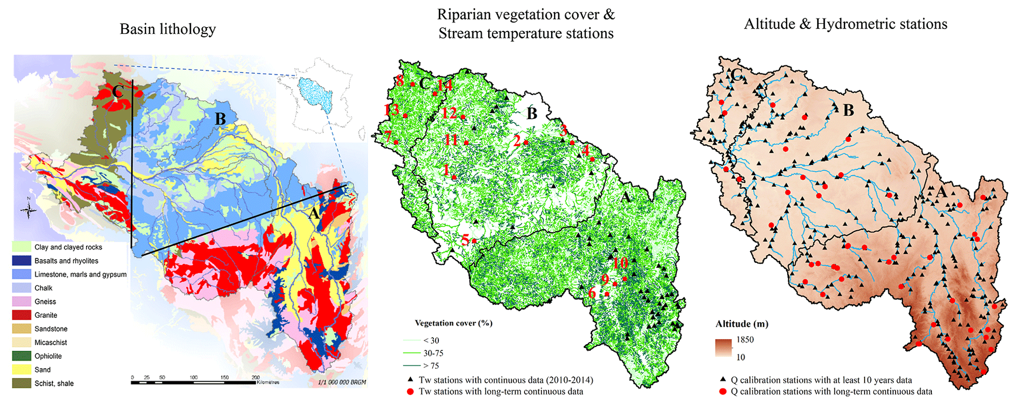
Figure 1Maps of the Loire basin. Left panel: basin lithology adapted from Moatar and Dupont (2016), based on original data from BRGM (French Geological Survey). The figure in the top right corner of the left panel shows the position of the Loire River basin in France. Middle panel: riparian vegetation cover (provided by Valette et al., 2012) and Tw stations. All Tw stations were used to assess the performance of the T-NET thermal model (see Table S5), but only the ones with long-term data (in red) were used to assess the T-NET thermal model accuracy for long-term trends. Complete information on Tw stations with long-term continuous data is provided in Table 1. The numbers in red in the middle panel correspond to the ID of long-term Tw stations in Table 1. Right panel: altitude (IGN, 2011) and hydrometric stations (extracted from the French national Banque Hydro database: http://www.hydro.eaufrance.fr/, last access: 12 July 2021). All hydrometric stations were used for calibrating the EROS hydrological model (see Table S2), but only stations on the French Reference Hydrometric Network (RHN) with long-term data (in red) were used to assess the EROS hydrological model performance on long-term trends (see Table S4).
We assessed how Tw responded to climate change over the past 57 years in the Loire River basin in four steps. First, we applied physically based Q and Tw models for the 1963–2019 period. Second, we assessed both hydrological and thermal model performance by comparing simulated seasonal and annual Q and Tw to data from observation stations. Third, we assessed Q and Tw long-term trends. Fourth, we analysed how hydroclimatic changes and landscape features could explain reconstructed trends in Tw. We performed all analyses on both seasonal and annual bases, where winter is December–February (DJF), spring is March–May (MAM), summer is June–August (JJA), and autumn is September–November (SON). Analyses were also performed by HER (see Fig. 1 and Sect. 2) to look at the large-scale influence of landscape characteristics.
3.1 Modelling daily Q and Tw
We used two models to calculate Tw in the Loire River basin according to the method developed by Beaufort et al. (2016). The first model is the EROS semi-distributed hydrologic model, which estimates daily Q at sub-basin outlets. The second model is the fully distributed, mechanistic temperature model called Temperature-NETwork (T-NET; Beaufort et al., 2016; Loicq et al., 2018) that uses Q from EROS and meteorological reanalysis data from Safran atmospheric reanalysis data (Quintana-Segui et al., 2008; Vidal et al., 2010) to estimate Tw at each reach in the Loire River basin. These models are briefly described below and are detailed in Thiéry (1988), Thiéry and Moutzopoulos (1995), and Thiéry (2018) for EROS and Beaufort et al. (2016) and Loicq et al. (2018) for T-NET.
3.1.1 EROS hydrological model principles and input data
The EROS semi-distributed hydrological model simulates daily Q at the outlet of 368 sub-basins (ranges between 40 and 1600 km2; mean drainage area = 300 km2), designed to be as homogeneous as possible with respect to land use and geology. On each of these sub-basins, the water balance is modelled by a lumped model using three reservoirs (see Fig. S2 in the Supplement) and a routing function for propagation across sub-basins (Thiéry, 1988; Thiéry and Moutzopoulos, 1995; Thiéry, 2018). Water abstractions are not considered in EROS, and it produces natural Q. This hydrological model has already been used in several other studies, including climate change impact studies (Ducharne et al., 2011; Habets et al., 2013; Bustillo et al., 2014).
EROS used daily Ta (∘C), solid and liquid precipitation (mm), and reference evapotranspiration (ET0, mm) to produce mean daily Q and groundwater flows (Thiéry, 1988; Thiéry and Moutzopoulos, 1995; Thiéry, 2018). Meteorological inputs were provided by the 8 km gridded Safran atmospheric reanalysis data released by Météo-France over the 1958–2019 period (Quintana-Segui et al., 2008; Vidal et al., 2010). ET0 was computed from Safran variables with the Penman–Monteith equation (Allen et al., 1998).
3.1.2 T-NET thermal model principles and input data
The T-NET thermal model is a fully mechanistic, 1D model that simulates hourly at distance, i, along reach, j, by solving the local heat budget. The heat budget of each reach includes six fluxes (W m−2): net solar radiation, atmospheric longwave radiation, longwave radiation emitted from the surface water, evaporative heat flux, convective heat flux, and groundwater flux. Briefly, the model calculates the longitudinal change in Tw at time t (d) for steady-state conditions in order to achieve thermal equilibrium (i.e. , where H is a heat flux) while accounting for confluence mixing. Detailed information about the T-NET model principles and calculation of the six heat fluxes at the water–air and water–stream bed interfaces and thermal propagation was provided in Beaufort et al. (2016) and Loicq et al. (2018).
The hydrographic network of the model over the Loire basin consists of 52 278 reaches delimited either by confluences of two streams or a headwater source (i.e. first-order reaches) (Beaufort et al., 2016; Loicq et al., 2018). The mean reach length is 1.7 km, and 74 % of the reaches have a Strahler order lower than 3 (see Fig. S3). To compute the six heat fluxes and the water travel time for each reach, the following input data were used.
-
Meteorological variables: hourly Ta (∘C), specific humidity (g kg−1), wind velocity (m s−1), shortwave radiation (W m−2), and longwave radiation (W m−2) were provided by the 8 km gridded Safran atmospheric reanalysis (Vidal et al., 2010). All reaches within a grid cell were assigned the values of the meteorological variables in that grid cell. For reaches flowing through more than one grid cell, meteorological variables were weighted by the relative length of the reach within each grid cell.
-
Riparian vegetation shading: riparian vegetation is one of the major regulators of shortwave radiation. In the current study, patches of wooded area provided by the BD TOPO® (IGN, 2008) database were used as a proxy of vegetation. The vegetation species and length of each wooded patch in a buffer of 10 m were extracted for both the right and left river banks (van Looy and Tormos, 2013). The vegetation density (vc) was then calculated as the ratio of patch length to reach length for both the right and left river banks. In the case of multiple wooded patches on any side of a river bank, the average vegetation density of the patches was considered. Then, the model proposed by Li et al. (2012) was used for the calculation of the dynamic shading factor (SF) at an hourly time step. The required average tree height for both the right and left river banks was estimated based on vegetation species (see Table S1).
In the presence of different vegetation species, the average tree height (m) for each side of a river bank was calculated as follows:
with Hi and Li the height and length of the tree patch i, respectively, and L the reach length. Next we calculated the proportion of the river width that was shaded (Wshaded) and the dynamic SF as follows:
where H is the average tree height (see Eq. 1), W is the river width (see Eq. 7), Ψ is the solar altitude angle, δ is the angle between solar azimuth and the mean azimuth of T-NET reach, and vc is the vegetation density. Loicq et al. (2018) already tested this method and showed that Tw simulated by the above method was close to the observed Tw. To take into account the phenology and stages of leaf growth, a coefficient corresponding to each season and transmissivity was applied to the SF to calculate the final shading factor: SF). The transmissivity in leafless months (January, February, November, and December), months of leaf growth (March and April), and full-leaf months (May–September) was fixed to 0.3, 0.2, and 0, respectively, following Hutchison and Matt (1977). The shortwave radiation was lastly regulated by a factor of 1−SFfinal.
-
Reach streamflow: the daily Q simulated at the outlet of 368 homogeneous sub-basins by the EROS model (see Sect. 3.1.1) was redistributed along the river network inside each sub-basin according to the reach drainage area for informing the T-NET model at the reach scale. The ratio of the sum of the lengths of all reaches upstream of a reach to the sum of the lengths of all reaches located in a sub-basin was used as a proxy for the drainage area of a reach. To have Q at an hourly time step, Q was assumed to be constant over 24 h.
-
River hydraulic geometry: stream depth and width were calculated using a hydraulic model assuming a rectangular river section being constant over 24 h (Morel et al., 2020):
with f and b being at-a-reach exponents previously predicted by climate, hydrological, topographic, and land use descriptors (see Morel et al., 2020, for more details). Q(t) is the daily mean streamflow provided by the EROS hydrological model. Q50, W50, D50 (the median of Q, width, and height, respectively), and the exponents were available on the Theoretical Hydrographic Network for France (RHT, Pella et al., 2012). There was about 50 % correspondence between the reaches of the T-NET and RHT networks. For the rest of them, required hydraulic geometry variables for the T-NET reaches were extrapolated from the nearest RHT reach. These river hydraulic geometries allowed us to calculate the water velocity by the ratio of Q(t) to rectangular wetted cross section. The travel time was also defined by the ratio of reach length to water velocity.
3.2 Model assessment and validation
3.2.1 Calibration and assessment of the EROS hydrological model
For calibration, 352 hydrometric stations with observed Q data (see Table S2) extracted from the French national Banque Hydro database (http://www.hydro.eaufrance.fr/, last access: 12 July 2021) were used (Fig. 1, right). Stations along the main Loire (14 stations) and Allier (11 stations) rivers were influenced by operations of four large dams for hydropower, flood control, and low-flow management, notably through summer releases (see Table S3). Time series at these stations were first naturalized by EDF (Électricité de France) based on variations in water storage in reservoirs due to operations based on target storage curves (Naussac, Villerest) and optimization of the hydropower energy generation for the electric grid needs (Grangent, Montpezat). EROS was then calibrated over the 1971–2018 period (which maximizes the number of available streamflow observations) against daily Q at all 352 sub-basins with at least 10 years of daily observations. Note that, in the current study, calibrating EROS by performing a classical split-sample test was not possible due to the numerous and diverse gaps in streamflow observations at this large scale. Therefore, calibration was done on the complete set of available information over the past decades, which is a standard approach for calibrating a hydrological model in climate change impact studies (e.g. Habets et al., 2013; Vidal et al., 2016).
The calibration aimed at optimizing all unknown parameters (soil capacity, recession times, and propagation times) by maximizing the Nash–Sutcliffe efficiency (NSE) criterion on the square root of streamflow and minimizing the overall bias. Considering the NSE criterion on the square root of the flows provided an estimate of model performance without favouring either high flows or low flows. The overall calibration criterion, C, was , where mNSE is the mean NSE, mRB is the mean relative bias, and w is a weighting factor fixed at 0.05. A 3-year warm-up period (1971–1974) was discarded from the overall calibration period for the next assessments.
The calibrated model was then used to simulate streamflow over all 368 homogenous sub-basins in the Loire basin over the whole 1963–2019 period. Note that, although meteorological variables were available from 1958 onwards, the first years (1958–1962) were discarded from the analysis to ensure the EROS model convergence.
Of the 352 calibration stations considered by EROS, 44 were part of the French Reference Hydrometric Network (RHN) described by Giuntoli et al. (2013) with long-term continuous high-quality data over the 1968–2019 period, especially for low flows (see Table S4). These stations are shown with red points in Fig. 1, right. Seasonal and annual relative biases, together with Nash–Sutcliffe efficiency on Q, ln (Q), and were computed on both 352 calibration (over the 1975–2018 period) and 44 RHN stations (over the 1968–2019 period) to provide an overview of the performance of the EROS model. Moreover, to assess EROS model ability to capture long-term trends, decadal trends (in percent per decade) over the 1963–2019 period on seasonal and annual averages from the EROS simulation were compared with corresponding observed trends at each of the 44 RHN stations with long-term continuous daily data.
3.2.2 Validation of the T-NET thermal model
T-NET does not consider the influence of impoundments on thermal energy balance and thus produces “natural” thermal regimes. Therefore, model performance was assessed on near-natural Tw stations, which are also weakly influenced by impoundments, i.e. at 67 stations with continuous daily data over the 2010–2014 period (see Fig. 1, middle, and Table S5). These stations were identified using the thermal signatures approach that allows one to distinguish between natural and altered thermal regimes (see Seyedhashemi et al., 2020, for more details). Of these identified natural stations, 55 were located on small/medium streams (with distance from the source < 100 km), while the rest were located on large rivers. The mean catchment area of natural stations was 151 km2 (range = 7–1342 km2) for small/medium streams and 18 926 km2 (range = 1931–57 043 km2) for large rivers. Tw data at these 67 stations were provided by different organizations: EDF, OFB (Office français de la biodiversité), DREAL (Direction régionale de l'environnement, de l'aménagement et du logement), and FD (Fédération Nationale de la Pêche) (see Tables 1 and S5). Tw data provided by OFB can be downloaded from http://www.naiades.eaufrance.fr/ (last access: 1 August 2020). The rest of the Tw data are not archived for public use. Seasonal and annual absolute biases and root mean square error (RMSE) were assessed at these 67 stations. Note that, unlike the EROS hydrological model, the T-NET thermal model does not have any free parameter, and hence it did not require calibration.
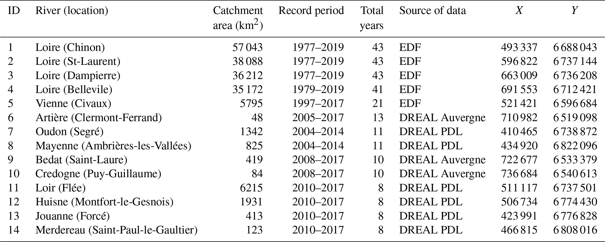
Long-term continuous data were available at 14 of the 67 near-natural stations, including 9 stations with 8–13 years of data and 5 stations with 20–40 years of data. These 14 stations are represented as red points in Fig. 1, middle panel, and listed in Table 1. The long-term evolution of annual mean Tw at these stations was shown in Fig. S4. These 14 near-natural stations with long-term continuous data comprised the validation data set for the seasonal and annual trend assessment (see Table 1).
Table 1Characteristics of the 14 long-term Tw stations. See Fig. S4 for the evolution of observed annual Tw at these stations. The IDs of stations correspond to the numbers (in red) shown in Fig. 1, middle. The coordinate system is Lambert 93.
3.3 Time series reconstruction and assessment of long-term trends
Daily Q and Tw were reconstructed over the 57-year period 1963–2019 using the EROS hydrological model and the T-NET thermal model. For each of the 52 278 reaches, daily time series of Ta (from the Safran reanalysis), Q (from EROS), and Tw (from T-NET) were reconstructed. Seasonal and annual averages of these three variables were considered in the trend assessment. Maps of annual mean Tw, Ta, and Q over the 1963–2019 period were presented in Fig. S5 with annual Tw > 11.5 ∘C for large rivers (annual Ta > 10.5 ∘C and log (annualQ)>1 m3 s−1).
We estimated the magnitude of trends in these time series with the non-parametric Theil–-Sen estimator (Sen, 1968) and evaluated their significance with the Mann–Kendall test (Mann, 1945) commonly used in hydrological analyses (see e.g. Giuntoli et al., 2013) but also thermal analyses (e.g. Kaushal et al., 2010; Arismendi et al., 2013a; Arevalo et al., 2020). This test is robust to non-normal data, non-linear trends, and series with outliers and missing values. Trend magnitudes were reported in ∘C decade−1 for Ta and Tw and in % decade−1 for Q (percentage of changes over the whole period) to help for comparisons across the basin.
3.4 Hydroclimatic drivers of Tw trends
Many factors affect the spatiotemporal variability of Tw. In the current study, we considered Ta as a proxy for heat fluxes and meteorological variables and Q as a proxy for thermal inertia and hydraulic geometries (which depends on Q; see Eqs. 6 and 7). To understand variability in Tw trends, we assessed spatial coherence and temporal synchronicity between trends in Tw and trends in Ta and Q as the main hydroclimate drivers influencing Tw. To do so, we first assessed the spatial coherence between these variables. In this regard, distributions of trends in Tw and Ta were first compared for the whole basin at the seasonal and annual scales using the non-parametric Wilcoxon signed rank test (Bauer, 1972) to determine whether median Tw trends were greater than median Ta trends. Then, the spatial coherence across reaches in terms of difference in trends between Tw and Ta on the one hand and sign of trend in Q on the other hand was assessed to explain the discrepancy between Tw and Ta found in the previous step with respect to Q.
Then, we assessed the temporal link between these three variables (i.e. Tw, Ta, and Q). To do so, for each identified reach, we first evaluated the strength and direction of joint trends using Pearson correlation between (i) Tw and Ta and between (ii) Tw and Q. Ta, Tw, and Q seasonal and annual anomalies – with respect to the 1963–2019 interannual mean – were then used to assess the synchronicity of extreme years and change points in time series. Change points in time series of anomalies at each reach were computed with the non-parametric Pettitt test that considers no change in the central tendency as a null hypothesis (Pettitt, 1979). Change points were reported at the 95 % confidence level.
3.5 Landscape drivers of Tw trends
Stream size, within individual large-scale homogeneous HERs, was selected as the first major potential landscape driver. The Strahler order of each reach was used as a proxy for stream size. Reaches with Strahler order 5–8 were combined into a single group termed “large rivers”. The Spearman correlation was computed between decadal trends in Tw (i.e. across all reaches) and Strahler order. Such correlations were computed across HERs and at seasonal and annual scales to evaluate the spatial heterogeneity and seasonality. Finally, in order to better illustrate the relationship between trends in Tw and Strahler order, median Tw trends of each group of rivers with respect to Strahler order were presented.
Second, the influence of riparian vegetation shading on trends in Tw was assessed using the daily average of the riparian vegetation shading (SF) simulated by T-NET. Seasonal shading was computed as the average of the daily SF over each season. For this analysis, only low-order reaches – distance from the source <30 km – were considered, based on previous observations that riparian shading primarily influences Tw at this scale (Dan Moore et al., 2005; Loicq et al., 2018). Then, as for the previous analysis for the influence of stream size, the correlation between decadal Tw trends and five levels of riparian shading (<15 %; 15 %–25 %; 25 %–40 %; 40 %–60 %; >60 %) was computed across HERs and seasons. Finally, median Tw trends were compared for each level of riparian shading.
4.1 Performance of models against observations
The EROS model performed well at the 352 calibration stations at the annual scale with a median relative bias close to 0 % (see Fig. S6, left). It slightly underestimated winter Q (median relative bias (across stations) %) and spring Q (−3.47 %) and overestimated summer Q (+34.7 %) and autumn Q (+20.9 %). The EROS model also performed well at 44 RHN stations with long-term continuous daily data at the annual scale with a median relative bias of 0.37 % (see Fig. S6, right). It slightly underestimated winter Q (median relative bias (across stations) %) and spring Q (−6.79 %) and overestimated summer Q (+37.7 %) and autumn Q (+24.7 %). The mean NSE criteria for Q, ln (Q), and were > 0.7 for at least 75 % of both calibration and RHN stations (see Fig. S7). A good performance of the EROS model in reconstructing daily Q was also seen at three different hydrometric stations located in the upstream, middle, and downstream parts of the Loire River basin (see Fig. S8).
No systematic bias was found for Tw modelled by T-NET at the stations located on small and medium rivers (see Fig. S9, top left). Median Tw bias ranged from −0.26 ∘C (in autumn) to 0.8 ∘C (in winter). Large rivers exhibited a small Tw underestimation (see Fig. S9, top right), with a median bias ranging from −0.29 ∘C (in autumn) to +0.15 ∘C (in winter), and the overall biases were still quite small across seasons (interquartile range (IQR) = 0.4–0.7 ∘C depending on season). On the other hand, the median RMSE of the T-NET thermal model, for small and medium rivers, ranged between 0.52 ∘C (in annual) and 0.91 ∘C (in DJF and JJA) across seasons (see Fig. S9, bottom left). For large rivers, the median RMSE of the T-NET thermal model ranged between 0.38 ∘C (annual) and 1.11 ∘C (SON) across seasons (see Fig. S9, bottom right). Moreover, 53 %–83 % stations (50 %–100 %) on small and medium (large) rivers had a RMSE < 1 ∘C across seasons.
Trends in observed and modelled Q were significantly correlated for all seasons (Fig. S10), with the highest correlation across stations found in spring and autumn (r=0.69 and 0.71, p< 0.05) and the lowest correlation found in summer, which was also non-significant (r=0.17, p=0.26). The trends of both modelled and observed Q were slightly decreasing (up to −11 % decade−1) for the majority of stations across all seasons, but the trend was significant for a very few of them (and mostly at the annual scale), all located in the southern part of the basin in HER A (red points of Fig. S10). Moreover, there were only a few discrepancies between estimates of trend significance in modelled and observed Q across seasons (11 %–18 % of stations).
Modelled and observed Tw trends also correlated significantly (see Fig. S11) across seasons, with the highest correlation in summer (r=0.94, p<0.001) and the lowest correlation in autumn, which was also non-significant (r=0.29, p=0.32). There was also good agreement between estimates of trend significance in modelled and observed Tw across seasons. Indeed, the trends in observed and simulated Tw were either both significant or neither was significant. Contrasting with trends in Q, trends for Tw increased for most stations across seasons, but the short period of record led to mostly non-significant trends. However, stations with long-term data showed significant increasing trends for all seasons, with the exception of winter (Fig. S11).
A visual comparison of observed and modelled Tw time series and trends at stations with long-term data (> 20 years) indeed suggested a strong coherence and agreement between observations and simulations provided by T-NET for all seasons (Fig. 2). For the four stations along the main stem of the Loire River (Fig. 2), the greatest increase occurred in spring – +0.61 (+0.71) ∘C decade−1 in observations (simulations) – and summer – +0.62 (+0.58) ∘C decade−1 in observations (simulations). The smallest increase was found in winter – +0.22 (+0.28) ∘C decade−1 in observations (simulations).
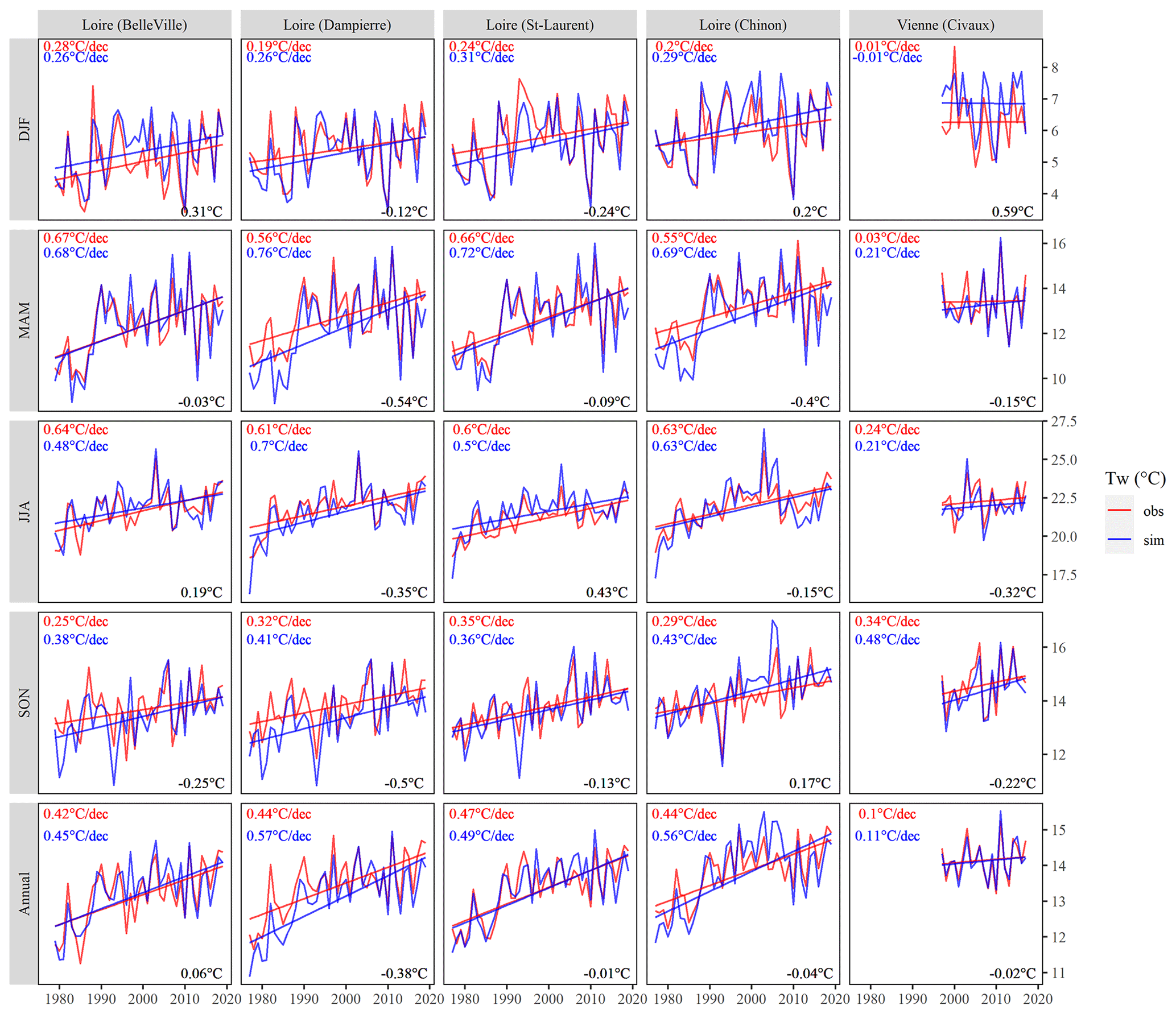
Figure 2Seasonal and annual time series of observed and simulated Tw at stations with at least 20 years of long-term continuous data between 1977 and 2019 (see Table 1 for more information). The red and blue solid lines show the trend in observed and simulated Tw. Numbers in red and blue in the top left corner of each graph show trend magnitudes (Sen's slope) in observed and simulated Tw. Numbers in black in the bottom right corner of each graph show the mean bias of the reconstruction.
4.2 Spatial reconstruction of long-term trends
Tw significantly increased in almost all modelled reaches for all seasons (Figs. 3, left, and S12, left). Depending on the season considered, 62 % to 80 % of reaches showed trends in the range of +0.2 to +0.4 ∘C decade−1 (i.e. +1.14 to +2.28 ∘C over the whole 1963–2019 period; see Fig. S13). Summer Tw trends were more spatially variable than in other seasons, with more than 50 % of reaches showing values higher than +0.4 ∘C decade−1 (see Fig. S13). Such reaches were mainly located in the southern part of the basin, in HER A (see Fig. 3, left). Spring Tw trends showed a similar spatial pattern but with lower trend values.

Figure 3Spatial variability of trends in seasonal and annual Tw, Ta, and Q over the 1963–2019 period based on Sen's slope estimator. Solid black lines show the Hydro-Ecoregion (HER) delineation (see Fig. 1). The statistical significance of these trends is given in Fig. S12.
Likewise, Ta exhibited increasing trends for 99 % of all reaches across spring, summer, and the whole year (Figs. 3, middle, and S12, middle). Values were mainly in the range of +0.2 to +0.4 ∘C decade−1 (see Fig. S13). The highest Ta trend values were found in summer and spring, when 67 % and 22 % of reaches, respectively, showed values higher than +0.4 ∘C decade−1. Such reaches were mainly located in HER A. Non-significant trends were found over the whole basin in winter and in the southern part of the basin in autumn.
In contrast to Ta and Tw, trends in Q were highly variable in magnitude and direction across the basin and across seasons (Fig. 3, right), and most were not significant at p=0.05 (Fig. S12, right). However, significant decreasing trends were found in the southern part of the basin (HER A) in spring, summer, and autumn and at an annual timescale (Fig. S12). Decreasing trends were observed for the majority of reaches across seasons (66 %–83 % of reaches), with the exception of winter (37 %) (see Fig. S14). Decreasing trends could have magnitudes greater than −5 % per decade, implying a −28 % loss in Q over the whole 1963–2019 period (see Fig. S14).
4.3 Hydroclimatic drivers of Tw trends
Spatial coherence
The medians of Tw trends were higher than those of Ta trends for every season (p<0.001 according to the Wilcoxon signed rank test), except for summer, when the median trend values for Tw and Ta were very similar, but more variable for Tw (+0.08 to +1.02 ∘C decade−1) (Fig. 4). The greatest increase in median Tw over the basin was found in summer (+0.44 ∘C decade−1).
Overall, Tw trends were more spatially variable than Ta trends (see Figs. 3 and 4), suggesting the conditional influence of other factors like Q trends. Indeed, for the majority of reaches, Tw trends exceeded Ta trends (see Fig. 5), with the exception of summer, when it was the case for half of the reaches. The difference between Tw and Ta trends could go up to 0.5 ∘C decade−1 (i.e. up to 2.85 ∘C over the whole 1963–2019 period) (see Fig. 5). At the majority of such reaches (where Tw trend > Ta trend), decreasing Q trends occurred coincidentally (43 %–94 % of all reaches) for all seasons (with the exception of winter), irrespective of whether all significant and non-significant trends were considered (Fig. 6, top) or only significant trends of all three variables (i.e. Tw, Ta, and Q) were considered (Fig. 6, bottom). Of these specific reaches where Tw trend > Ta trend and Q trend < 0, most were located in HER A (see Figs. S15 and S16). Moreover, wherever Tw trend < Ta trend, increasing Q trends occurred coincidentally (see the dark blue bars in Fig. 6), suggesting again the influence of Q trends as a possible explanation for discrepancies found between Tw and Ta trends.
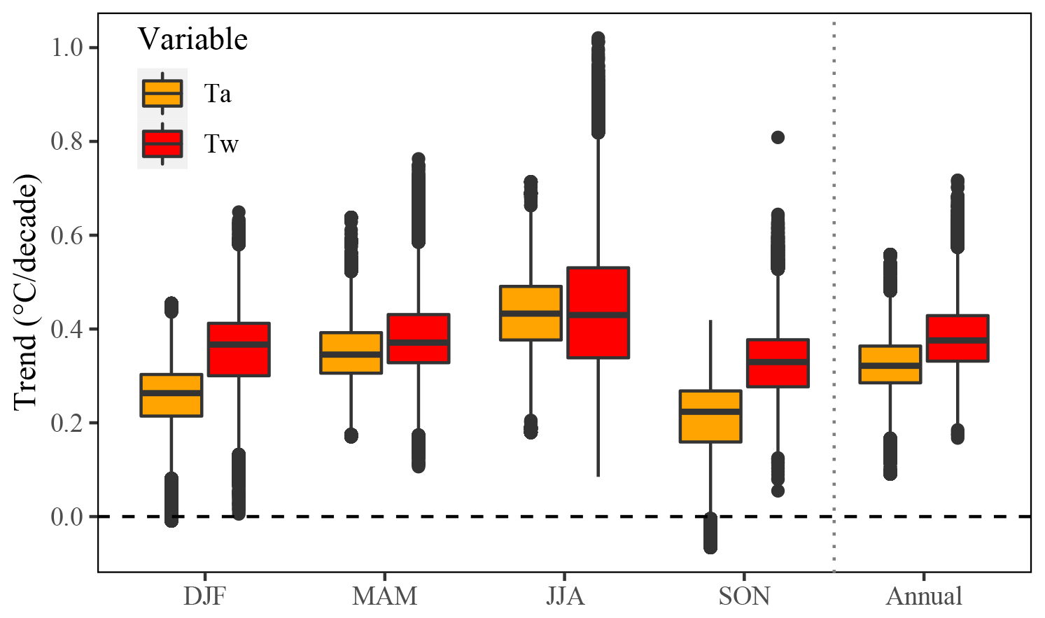
Figure 4Distributions of seasonal and annual trends in Tw and Ta for all 52 278 reaches over the 1963–2019 period. Sen's slope is used as the trend value estimate (see text). This representation includes both significant and non-significant trends.
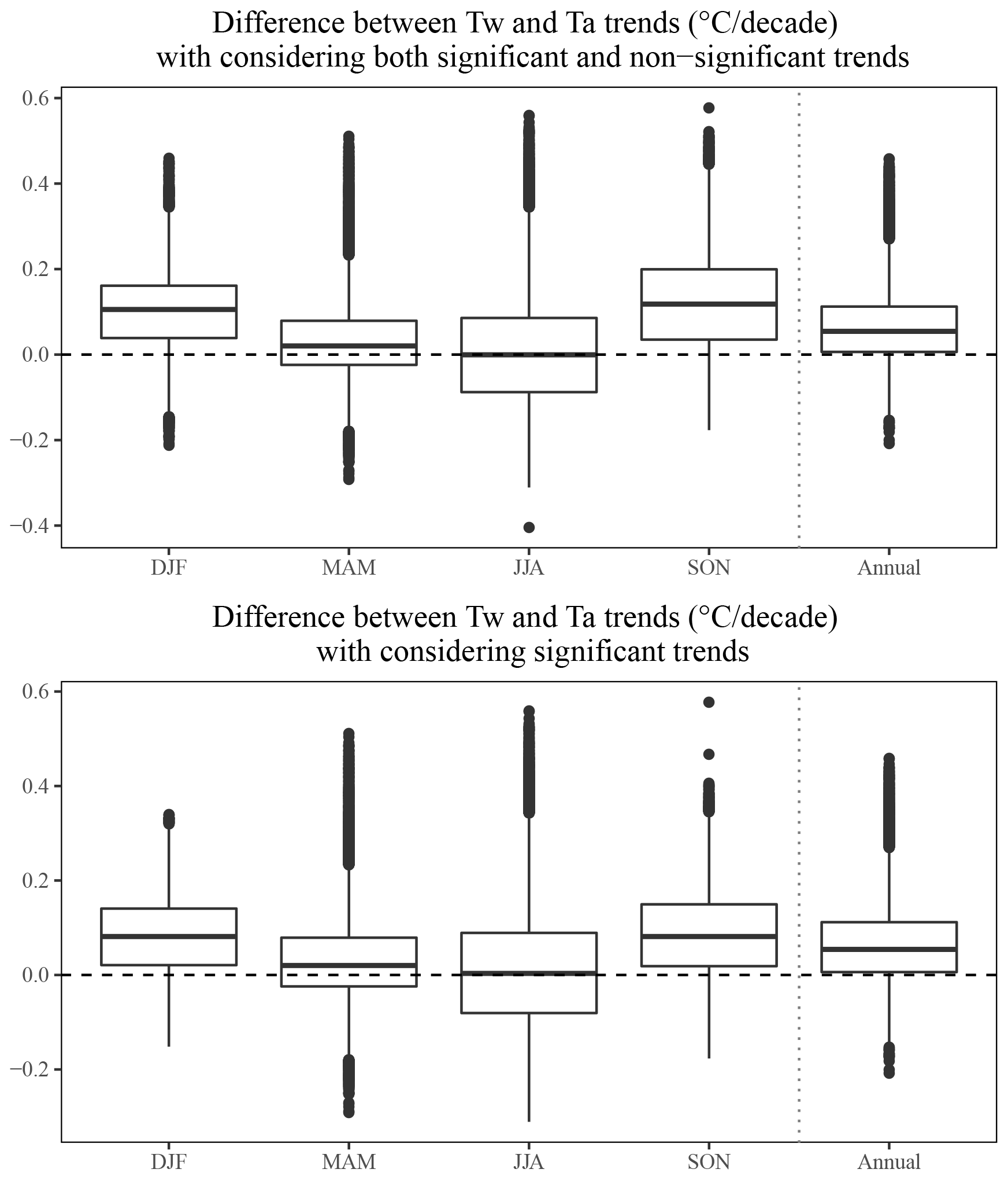
Figure 5Difference between Tw and Ta trends at each reach in ∘C per decade for all 52 278 reaches.
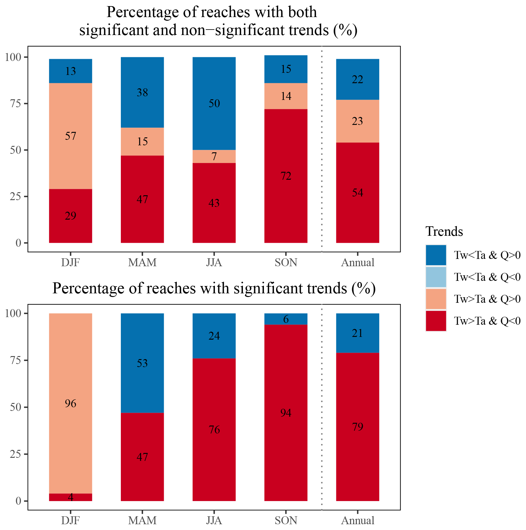
Figure 6Percentage of reaches with consistent 1963–2019 trends in Tw, Ta, and Q, categorized with respect to two criteria: (1) comparison between the Tw and Ta trends and (2) sign of the Q trend. Sen's slope is used as the trend value estimate.
Temporal synchronicity
We observed strong positive correlations between seasonal and annual averages of Tw and Ta across seasons ( to +0.82 depending on the season; see Table 2). We further observed a strong negative correlation between summer Tw and Q time series ().
Table 2Pearson correlation over the 1963–2019 period between seasonal and annual Tw and Ta and/or Q time series, averaged over all reaches. Percentages in brackets show the proportion of reaches with a significant correlation at the 95 % confidence level.
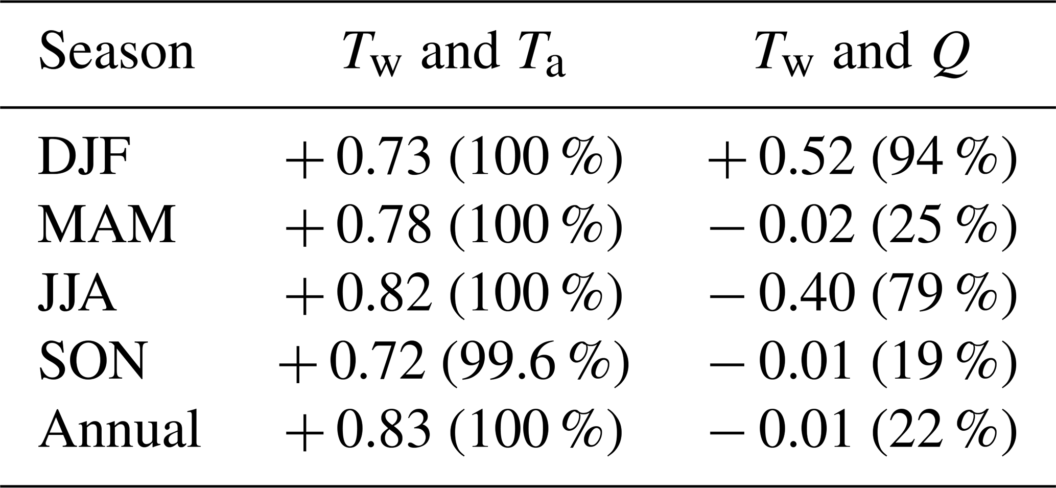
Annual anomalies of Tw, Ta, and Q exhibited variable patterns, with Tw and Ta generally increasing and Q remaining relatively stationary (Fig. S17). Tw anomalies were generally more variable than Ta, especially in summer, but both time series appeared to exhibit synchronous behaviour. Change-point analysis supported this visual observation, where change points in seasonal and annual averages were largely coincident across these time series (Fig. 7). Tw and Ta anomalies exhibited clear negative-to-positive change points in the late 1980s at nearly all reaches, with median values increasing by approximately +2 ∘C after the change point. These change points were observed in all seasons but were most pronounced and synchronous around 1988 in spring and summer. The change points detected in winter Tw and Ta time series were less concomitant, occurring mostly in the early 1990s (1992 and 1993) for Tw and in the late 1980s (1986–1989) for Ta. The autumn change points were distributed between 1980 and 1994 for both Tw and Ta. The significant change points in seasonal Q time series were detected for a substantially smaller proportion of reaches, e.g. fewer than 40 % of reaches for spring and summer. The majority of these reaches were located in HER A across seasons (66 %–86 % of such reaches), with the exception of winter (49 %) (see Fig. S18). In spring and summer, they occurred in the late 1980s, similarly to Tw and Ta. Conversely, the significant change points detected in other seasons were much more scattered in time, probably due to the high interannual variability of Q.
Critically, the largest summer Tw and Ta positive anomalies over the study period were observed in 1976, 1994, 1995, 2003, 2005, 2006, 2015, 2017, 2018, and 2019, which corresponded to years with the largest negative anomalies in summer Q, with the exception of 1994 and 2018 (Fig. 8). Note that this signal was much less clear for the other seasons (see Fig. S19).
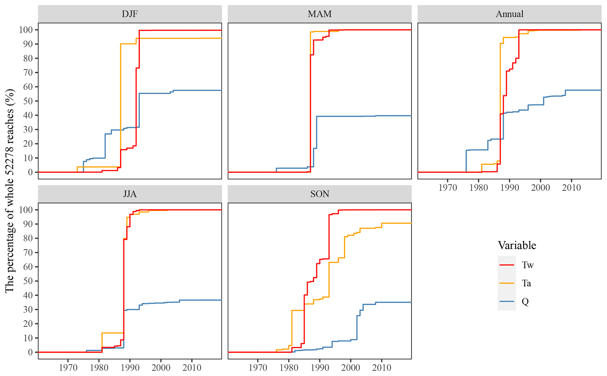
Figure 7Change points in Tw, Ta, and Q time series at the seasonal and annual scales, plotted as a proportion of reaches experiencing a shift in a given year. Only the first change point detected at the 95 % confidence level is considered, and non-significant change points were removed, leading to curves not reaching 100 %.
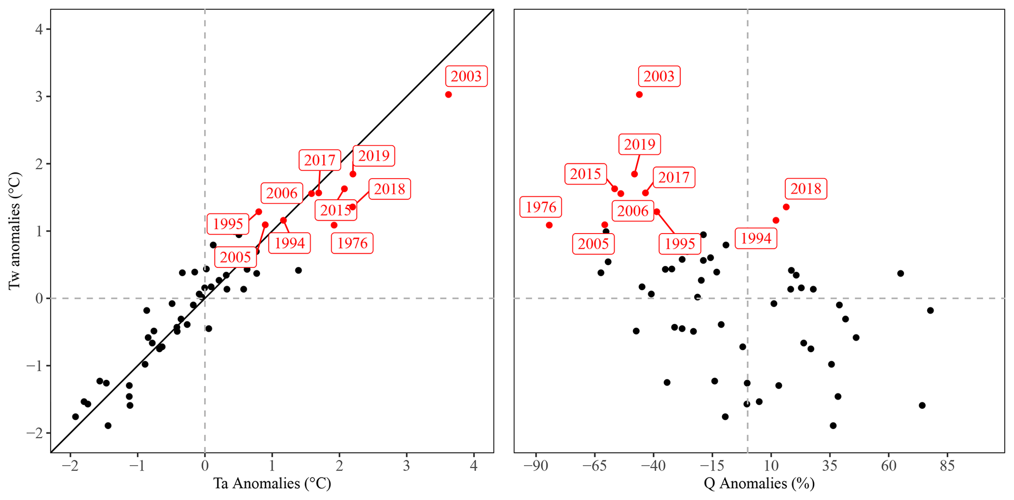
Figure 8Relationship between summer anomalies in Tw and Ta on the one hand and summer Tw and Q anomalies on the other hand. Individual years are identified from their median values across all reaches. Years with the highest anomalies in Tw ( ∘C) and corresponding anomalies in Ta and Q are identified in red.
4.4 Landscape drivers of Tw trends
4.4.1 Stream size and HER
Strahler order was strongly (p<0.001) and positively correlated with Tw trends for all HERs in spring and for HER A in summer and autumn and at the annual scale. HER A exhibited the highest positive correlations in spring () and summer () (Fig. S20). In other words, larger rivers tended to exhibit the largest increases in spring and summer Tw, especially for reaches located in HER A. There, median trends in spring (summer) ranged from +0.37 to +0.55 ∘C decade−1 (from +0.49 to +0.64 ∘C decade−1) from small streams (Strahler order 1) to large rivers (Strahler order ≥5).
4.4.2 Riparian shading and HER
For small streams, i.e. reaches located closer than 30 km from the source, the SF and trends in Tw were significantly (p<0.001) and negatively correlated in HER A in all seasons as well as in HER B and C in spring and in HER B in autumn (Fig. 9). Indeed, across seasons, the highest negative correlation was found in HER A ( to −0.37 depending on the season). Unsurprisingly, the mitigating effect of shading on trends in Tw for small streams was observed for all HERs in spring and only for HER A in summer and, to a lesser extent, in autumn and winter. The median spring Tw trend was mitigated by 0.12 ∘C decade−1 from sparsely shaded reaches (SF <15 %) to highly shaded reaches (SF >40 %). For summer Tw in HER A, the median trends were mitigated by 0.16 ∘C decade−1 from the lowest shaded reaches to the highest shaded reaches.
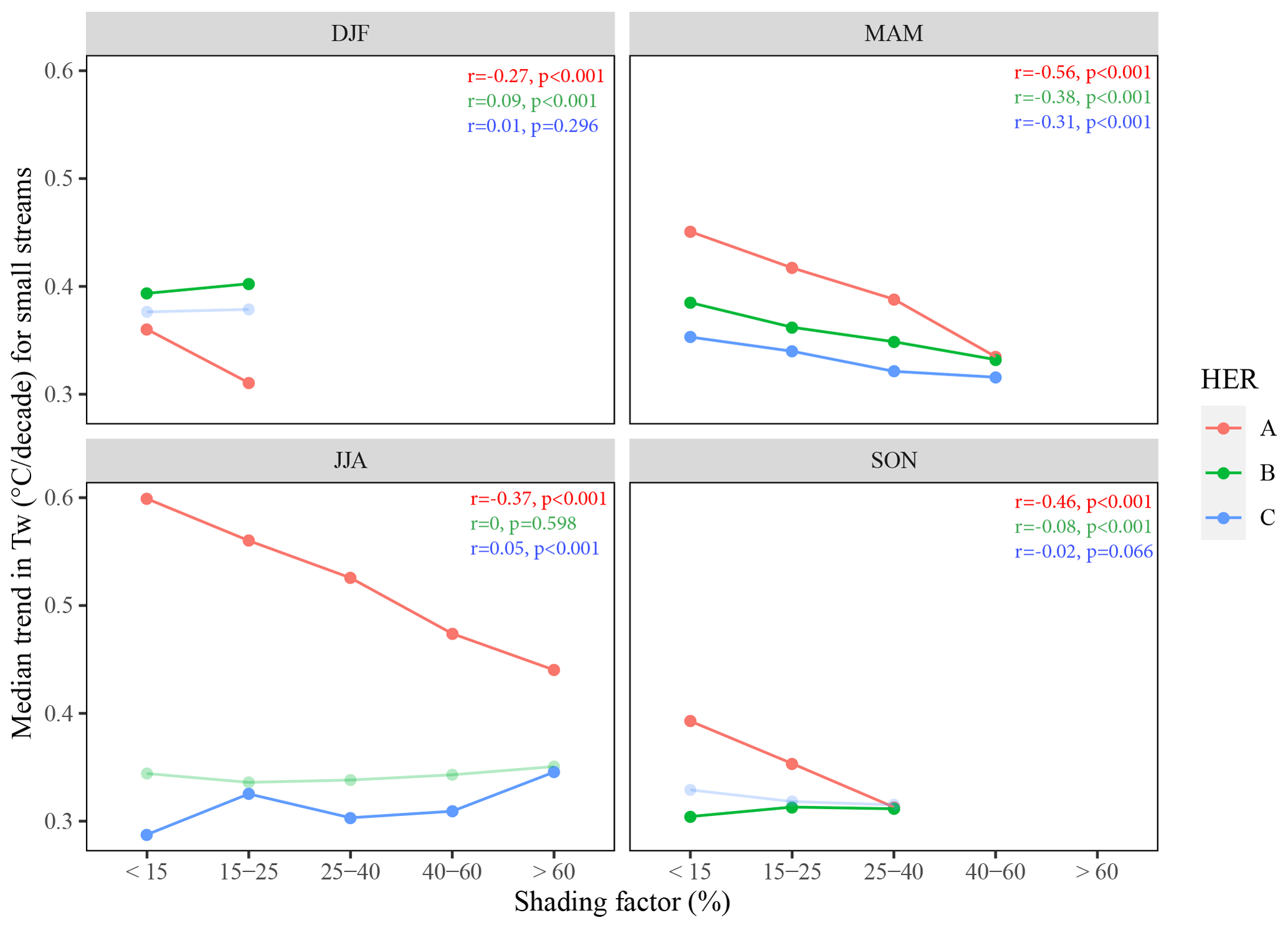
Figure 9Relationships between shading factor and median trends in Tw over the 1963–2019 period for small streams, by HER and by season. Note that some shading factor classes are not observed in autumn and winter. Correlations and associated p values are shown in the top right corner of each graph, and significant relationships at the 95 % confidence level are identified by full solid lines.
5.1 Quality and suitability of simulated Tw and Q
Although some biases were observed for both Q (Fig. S6) and Tw (Fig. S9), we found significant correlations between modelled and observed trends in seasonal and annual Q, with the exception of summer (Fig. S10), and Tw, with the exception of autumn (Fig. S11). The low correlation value found in summer Q (Fig. S10) originated from poor simulation at very few stations, all located in HER B. Two of these stations gauged catchments where numerous small ponds were found, and the highly decreasing observed trends might be due to the increasing evaporation from these ponds, which were obviously not included in the EROS hydrological model. This was also true to a lesser extent for the other hydrometric station, in which a canal followed a large part of the course of the river and might play a similar role with respect to summer evaporation trends. Apart from these specific stations, in summer, a coherence as good as in other seasons was found between trends in simulated and observed Q. Moreover, the spatial pattern in simulated Q trends, with significant decreases in the southern headwaters, was consistent with observations at the high-quality reference hydrometric stations (Giuntoli et al., 2013).
The low correlation between simulated and observed Tw trends found in autumn (Fig. S11) originated from two stations with 8–13 years of Tw data, while such correlation was really good at stations on the Loire and Vienne rivers with longer (20–40 years) Tw data. Therefore, poor correlation in autumn could be due to insufficient Tw data at these two stations. Moreover, consistent with Moatar and Gailhard (2006) and Arevalo et al. (2020), we found no trend (p>0.05) in both observation and simulation on the Loire (Dampierre) in winter.
5.2 Comparison with Tw trends in other European basins
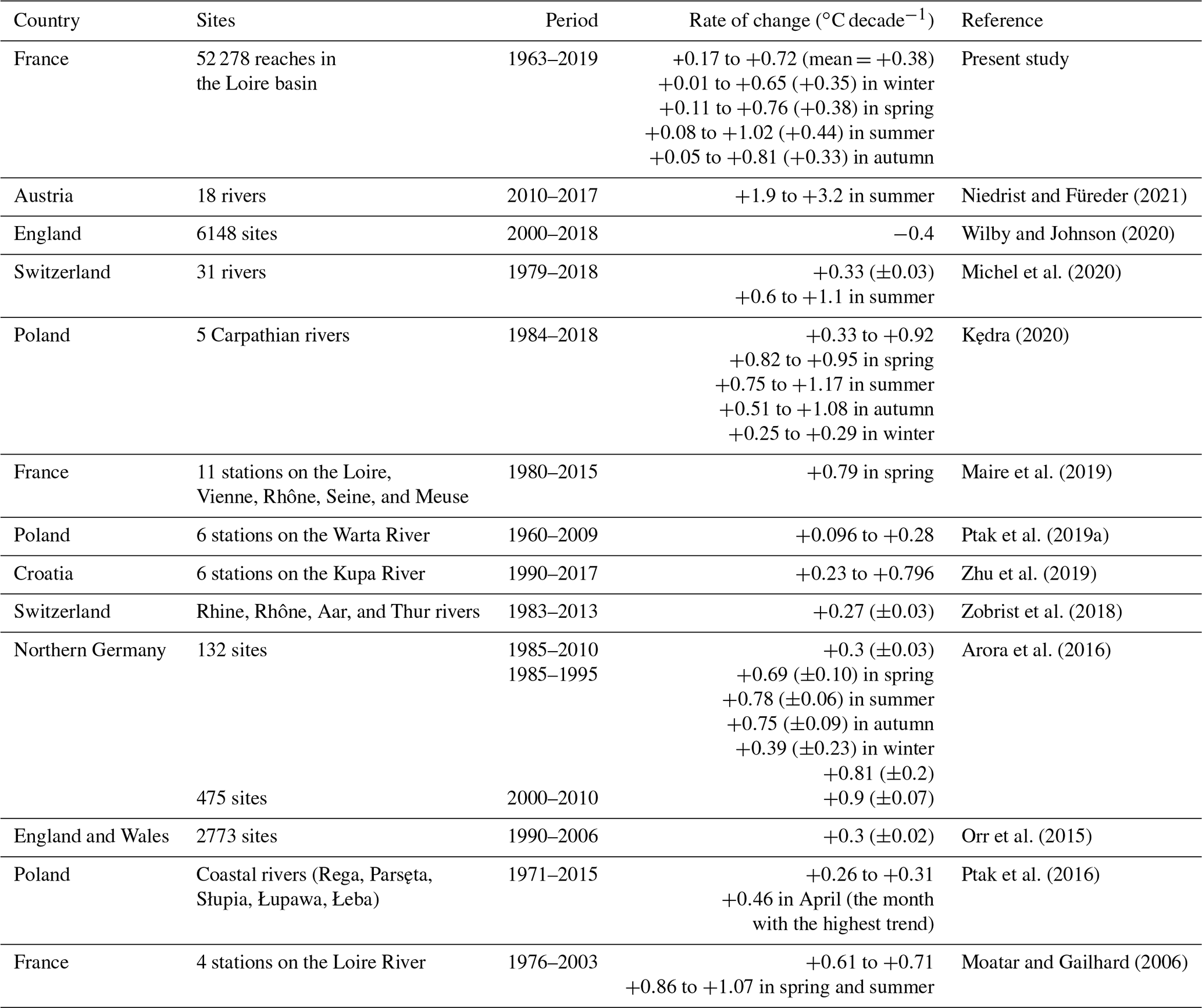
T-NET simulations over the 1963–2019 period showed significantly increasing trends in Tw for almost all reaches over the Loire basin across seasons (see Figs. 3, left, and S12, left), with an increase of +0.38 ∘C decade−1 on average at the annual scale. To the best of the authors' knowledge, the present study was one of the few studies using modelled Tw to investigate past trends at a large scale (but see Van Vliet et al., 2011; Isaak et al., 2012, 2017). Table 3, summarizing recently published findings based on observations, demonstrates that the present results are consistent with trends observed in other European basins, with clear increases in Tw over the recent decades. It also shows that the much larger scale and finer spatial resolution of the current study clearly stands out as unique. Although start year, end year, and length of the study period can have a significant influence on trend estimates and trend detection (Arora et al., 2016), comparing trends with other studies conducted over different periods gives us a comprehensive view of the overall magnitude of changes in Tw and possible related drivers.
Niedrist and Füreder (2021)Wilby and Johnson (2020)Michel et al. (2020)Kędra (2020)Maire et al. (2019)Ptak et al. (2019a)Zhu et al. (2019)Zobrist et al. (2018)Arora et al. (2016)Orr et al. (2015)Ptak et al. (2016)Moatar and Gailhard (2006)Table 3Recent studies on Tw trends in Europe. A comprehensive review of the relevant literature published prior to 2016 can be found in Arora et al. (2016). Magnitudes with unspecified seasons are related to the annual scale. Note that, except for the present study, the others used observed Tw.
Global-scale stream temperature modelling suggests trends in annual averages ranging from +0.2 to +0.5 ∘C decade−1 over France (Wanders et al., 2019), which is consistent with our findings (mostly in the range of +0.2 to +0.4 ∘C decade−1, Fig. S13). We found more pronounced trends in spring and summer, which was also found in other parts of Europe (e.g. Kędra, 2020; Arora et al., 2016; Michel et al., 2020). Considerable discrepancies were also found between Tw and Ta trends across seasons for the majority of the reaches (see Figs. 3 and 5), which is a common finding for other sites around the world (Arora et al., 2016; Wanders et al., 2019). This highlights that changes in Ta may not be the only driver of changes in natural Tw.
5.3 Drivers and spatial patterns of trends in Tw
Consistent with our findings (see Fig. 5), Moatar and Gailhard (2006) found Tw increased more quickly than Ta in spring and summer and at the annual scale for all four stations on the Loire River. Arora et al. (2016) also found Tw trends > Ta trends in summer. In Switzerland, Michel et al. (2020) described an increase of ∘C decade−1 in Tw, resulting from the joint effects of an increase in Ta ( ∘C decade−1) and a decrease in Q ( % decade−1) over the 1979–2018 period. In contrast with our results, they found Tw trends lower than Ta trends due to the influence of snowmelt and glacier melt in Alpine catchments. Consistent with their findings, Orr et al. (2015) also found Tw trends < Ta trends in the UK. They suggested that such differences between Tw and Ta trends could be a result of different processes driving Tw. In the current study, we found spatial coherence between trends in Tw and trends in Ta and Q. Indeed, the greatest increases in Tw (up to +1 ∘C decade−1) were predominately located in the southern part of the basin, in HER A (Massif Central), where a greater increase in Ta (up to +0.71 ∘C decade−1) and a greater decrease in Q (up to −16 % decade−1) occurred jointly. We also found, at the majority of reaches where Tw trend > Ta trend, decreasing Q trends occurred coincidentally for all seasons (with the exception of winter) (Fig. 6).
The decrease in Q could itself be due to a significant increase in PET (up to +10 %) over the whole basin and a decrease in total precipitation (P) (up to −5 % decade−1) (Figs. S21 and S22). Such trends, computed here based on variables from the Safran surface meteorological reanalysis (Vidal et al., 2010), are consistent with larger-scale studies (see e.g. Spinoni et al., 2017; Tramblay et al., 2020; Hobeichi et al., 2021). Moreover, Vicente-Serrano et al. (2019) attributed annual streamflow trends in southern France mostly to trends in precipitation and potential evapotranspiration, as opposed to irrigation and land-use changes that have additional strong effects, e.g. in the Iberian Peninsula. We also observed, for the majority of reaches where Tw increased less than Ta, an increase in Q that occurred jointly, suggesting that an increase in Q or in other words an increase in thermal inertia could also explain the discrepancy between Tw and Ta trends at these reaches (see Fig. 6).
A strong synchronicity between Ta and Tw anomalies was observed in the present study in the warmest years, and these years were also among those with the largest negative Q anomalies (see Fig. 8). Indeed, increase in summer Tw could be due to co-occurrence with the increase in summer Ta (average correlation: +0.82) and with the decrease in summer Q (average correlation: −0.40). These findings are consistent with those of Michel et al. (2020): average Tw–Ta correlation +0.61 and average Tw–Q correlation −0.66. For the middle Loire River, Moatar and Gailhard (2006) found that the increase in Ta (decrease in Q) explains 60 % (40 %) of the increase in Tw. Moreover, the significant change point in Tw, Ta, and Q time series in the late 1980s has also been found in other studies in Europe (Moatar and Gailhard, 2006; Arora et al., 2016; Zobrist et al., 2018; Ptak et al., 2019b; Michel et al., 2020). Long-term observational Tw time series like the Loire at Dampierre also displayed a similar change point.
Trends in Tw might also be explained by trends in additional drivers (not considered directly in the current study), like shortwave radiation (Wanders et al., 2019), which is the dominant flux at the air–water surface and is notably increasing over Europe (Sanchez-Lorenzo et al., 2015). This might explain why Tw increased more quickly than Ta in spring, summer, and autumn, when no decreasing trends in Q were found (see Fig. 6).
The current study suggests that Ta and Q could exert a joint influence on Tw, based on an analysis of the spatial coherence and temporal synchronicity of these variables. Assessing the causal influence of these factors on Tw trends goes beyond the scope of this paper and is left for future research. In this regard, one could devise a formal attribution framework where one may e.g. remove trends in Q and trends in Ta alternatively in T-NET inputs.
5.4 Natural trends and anthropogenic influence on Tw
Natural Tw time series were used in the current study for detecting trends, as both the EROS and T-NET models are used in a non-influenced set-up (see Sect. 3.1). However, anthropogenic impoundments (e.g. large dams, small reservoirs, and ponds) influence downstream Tw regimes in a variety of ways that depend on their structure and position along the river continuum (Seyedhashemi et al., 2020). In this regard, on the one hand, large dams, by releasing cold hypolimnetic water in summer, can lower downstream Tw (Olden and Naiman, 2010) and mitigate the increasing trend in Tw (Cheng et al., 2020). Nevertheless, it is anticipated that a considerable proportion of streams regulated by large dams may still experience high temperatures and low flows under future climate change (Cheng et al., 2020). The mitigating influence of dams could be of importance for streams in the southern headwaters of the Loire basin since this area both experienced the greatest Tw trends and gathers most of the existing large dams.
On the other hand, ponds and shallow reservoirs, by releasing warm water, can increase downstream Tw (Chandesris et al., 2019; Seyedhashemi et al., 2020; Zaidel et al., 2020) and exacerbate increasing trends in Tw (Wanders et al., 2019; Michel et al., 2020). The warming effect of such surface waters in the current study can be significant for streams located in lowlands in the middle and north of the Loire River basin, where most of the shallow reservoirs and ponds are located. In these streams, anthropogenically induced trends in Tw may be greater than natural ones, and the warming process can get worse through the increasing demand for storing water in small reservoirs for irrigation. Nevertheless, the warming effect can also be local, and streams located closer to such regulated streams may show limited to no warming (Wanders et al., 2019).
Note that, although there are nuclear power plants in the Loire basin, their impacts on Tw are considered negligible according to Moatar and Gailhard (2006) and Bustillo et al. (2014). Moreover, it was observed in the current study that the Tw trend at Belleville located upstream of power plants and, consequently, not influenced by them had the same trend magnitude as the other three stations located downstream (see Fig. 2), showing a negligible influence of nuclear power plants on Tw trends.
5.5 Implications for river management and aquatic biota
The removal of riparian vegetation can increase Tw (Caissie, 2006), and changes in Tw can be even more sensitive to changes in riparian vegetation than to changes in Ta or Q (Wondzell et al., 2019). We showed that, in small streams, an increase of > 25 % of riparian shading (from 15 % to 40 %) could mitigate the median trend in spring and summer Tw by up to 0.16 ∘C decade−1 (Fig. 9). Spring and summer Tw trends were more pronounced in large rivers, especially in the south of the basin, with a difference in median Tw trends of up to +0.18 ∘C decade−1 (Fig. S20), probably due to a decrease in Q (up to −2 % decade−1; see Fig. S23), a greater thermal sensitivity, and the absence of mitigating factors like riparian vegetation shading or groundwater inputs (Kelleher et al., 2012; Beaufort et al., 2020).
Restoring riparian vegetation and shading can therefore substantially mitigate future increases in Tw. In addition, riparian restoration may lessen the impacts of climate change on flood damage to human infrastructure, on riparian biodiversity, on ecosystem vulnerability, and on changes in Q (Palmer et al., 2009; Seavy et al., 2009; Perry et al., 2015). However, riparian restoration is not an easy task since the survival, persistence, growth rate of planted trees, as well as required time for thermal regime recovery under possibly severe future conditions should be studied beforehand (Perry et al., 2015). For instance, it may take between 5 and 15 years for rivers to recover their thermal regime following vegetation growth (Edmonds et al., 2000; Caissie, 2006). Moreover, the efficacy of riparian planting is also highly dependent upon the type and structure of forest stands (Dugdale et al., 2018), and this should also be considered in long-term projects.
Stream warming affects cold‐water fish populations negatively at the warmer boundaries of their habitat (Hari et al., 2006). Furthermore, changes in spawning and migration timing (McCann et al., 2018; Arevalo et al., 2020), decreases in habitat availability and freshwater quality for organisms (Lennox et al., 2019), and shifts in species distribution (Comte et al., 2013) are already observed as consequences of the long-term increase in Tw. Some major changes in fish density and community structure have already been reported in large rivers over France (Maire et al., 2019), for which we also found greater trends in Tw compared with small ones. Therefore, physical process-based thermal models like T-NET can also be used to assess the various stresses on freshwater habitat sustainability due to changes in Q and Tw (Morales-Marín et al., 2019).
Regional trends in Tw at the reach resolution were detected and assessed by using the T-NET physical process-based model coupled with the EROS hydrological model over the Loire basin. Using model outputs across 52 278 reaches over the Loire basin for three variables (Ta, Q, and Tw) and five timescales (seasons plus annual), we found consistent increasing Tw trends at the scale of the entire Loire River basin, regardless of the season. Critically, the rate of warming for stream temperature was in the majority of reaches higher than the rate of atmospheric warming, suggesting a decoupling of thermal trajectories linked to decreasing Q, especially in the southern part of the basin, supported by observed coherent spatial and temporal patterns and well-understood physical processes. Moreover, in the southern part of the basin, Tw trends in all seasons except winter were greater in rivers with Strahler order ≥5, which we attributed to the mitigation effect of riparian shading for small rivers.
The synchronicity of extreme events of low flows and high stream temperature in the southern part of the basin will likely generate a double penalty for existing cold-water aquatic communities. However, riparian shading in small streams in the southern part of the basin may mitigate such warming. These findings underscore that air temperature alone is likely not an adequate proxy for explaining stresses and shifts experienced by aquatic communities over time and space, especially in regions with more pronounced stream warming, and thus there is a need to grow and maintain Tw sensor networks. It also highlights that the physical process-based thermal models like T-NET can be used to assess the various stresses on freshwater habitat sustainability due to changes in Q and Tw. This knowledge can help develop appropriate management strategies to conserve thermal refugia and mitigate extreme thermal events induced by climate change.
The seasonal and annual Tw and Q time series at 67 stations (see Tables 1 and S5) can be downloaded from https://doi.org/10.15454/PTY9R7 (Seyedhashemi et al., 2022). Data for other reaches in the basin and codes are available from the corresponding author, Hanieh Seyedhashemi, upon reasonable request.
The supplement related to this article is available online at: https://doi.org/10.5194/hess-26-2583-2022-supplement.
The paper has been authored by HS with contributions from all the co-authors. HS, JPV and FM contributed to the conceptualization and methodology. HS ran the T-NET model and performed the formal analysis. DT ran the EROS model and provided simulated streamflow data. CM and FH provided long-term data on observed stream temperature and naturalized streamflow data. JPV, JSD, AM, DT and FM contributed to the writing and revision of the manuscript.
The contact author has declared that neither they nor their co-authors have any competing interests.
Publisher’s note: Copernicus Publications remains neutral with regard to jurisdictional claims in published maps and institutional affiliations.
The SAFRAN database was provided by the French national meteorological service (Météo-France). We are grateful to Electricité de France (French Electricity, EDF) for providing long-term data on observed stream temperature and naturalized streamflows. We also thank André Chandesris for his assistance in the incorporation of vegetation cover into the T-NET thermal model. We also thank Rohini Kumar, the editor of Hydrology and Earth System Sciences, and Adrien Michel and two anonymous referees for reviewing this article.
This work was realized in the course of a doctoral project at the University of Tours, funded by the European Regional Development Fund (Fonds Européen de développement Régional-FEDER), POI FEDER Loire (grant no. 2017-EX001784), Le plan Loire grandeur nature, AELB (Agence de l’eau Loire-Bretagne), INRAE (l'Institut national de recherche pour l’agriculture, l’alimentation et l’environnement), and EDF (Hynes team).
This paper was edited by Rohini Kumar and reviewed by Adrien Michel and two anonymous referees.
Allen, R. G., Pereira, L. S., Raes, D., and Smith, M.: Crop Evapotranspiration – Guidelines for computing crop water requirements, FAO Irrigation and Drainage Paper 56, FAO, https://appgeodb.nancy.inra.fr/biljou/pdf/Allen_FAO1998.pdf (last access: 11 May 2022), 1998. a
Arevalo, E., Lassalle, G., Tétard, S., Maire, A., Sauquet, E., Lambert, P., Paumier, A., Villeneuve, B., and Drouineau, H.: An innovative bivariate approach to detect joint temporal trends in environmental conditions: Application to large French rivers and diadromous fish, Sci. Total Environ., 748, 141260, https://doi.org/10.1016/j.scitotenv.2020.141260, 2020. a, b, c, d
Arismendi, I., Johnson, S. L., Dunham, J. B., Haggerty, R., and Hockman-Wert, D.: The paradox of cooling streams in a warming world: regional climate trends do not parallel variable local trends in stream temperature in the Pacific continental United States, Geophys. Res. Lett., 39, 10, https://doi.org/10.1029/2012GL051448, 2012. a
Arismendi, I., Johnson, S. L., Dunham, J. B., and Haggerty, R.: Descriptors of natural thermal regimes in streams and their responsiveness to change in the Pacific Northwest of North America, Freshwater Biol., 58, 880–894, https://doi.org/10.1111/fwb.12094, 2013a. a
Arismendi, I., Safeeq, M., Johnson, S. L., Dunham, J. B., and Haggerty, R.: Increasing synchrony of high temperature and low flow in western North American streams: double trouble for coldwater biota?, Hydrobiologia, 712, 61–70, https://doi.org/10.1007/s10750-012-1327-2, 2013b. a
Arismendi, I., Safeeq, M., Dunham, J. B., and Johnson, S. L.: Can air temperature be used to project influences of climate change on stream temperature?, Environ. Res. Lett., 9, 084015, https://doi.org/10.1088/1748-9326/9/8/084015, 2014. a
Arora, R., Tockner, K., and Venohr, M.: Changing river temperatures in northern Germany: trends and drivers of change, Hydrol. Process., 30, 3084–3096, https://doi.org/10.1002/hyp.10849, 2016. a, b, c, d, e, f, g, h, i, j, k
Bauer, D. F.: Constructing confidence sets using rank statistics, J. Am. Stat. Assoc., 67, 687–690, https://doi.org/10.1080/01621459.1972.10481279, 1972. a
Beaufort, A., Curie, F., Moatar, F., Ducharne, A., Melin, E., and Thiéry, D.: T-NET, a dynamic model for simulating daily stream temperature at the regional scale based on a network topology, Hydrol. Process., 30, 2196–2210, https://doi.org/10.1002/hyp.10787, 2016. a, b, c, d, e
Beaufort, A., Moatar, F., Sauquet, E., Loicq, P., and Hannah, D. M.: Influence of landscape and hydrological factors on stream–air temperature relationships at regional scale, Hydrol. Process., 34, 583–597, https://doi.org/10.1002/hyp.13608, 2020. a
Benyahya, L., Caissie, D., St-Hilaire, A., Ouarda, T. B., and Bobée, B.: A review of statistical water temperature models, Can. Water Resour. J., 32, 179–192, https://doi.org/10.4296/cwrj3203179, 2007. a
Blöschl, G., Hall, J., Viglione, A., Perdigão, R. A., Parajka, J., Merz, B., Lun, D., Arheimer, B., Aronica, G. T., Bilibashi, A., and Boháč, M.: Changing climate both increases and decreases European river floods, Nature, 573, 108–111, https://doi.org/10.1038/s41586-019-1495-6, 2019. a
Bruno, D., Belmar, O., Maire, A., Morel, A., Dumont, B., and Datry, T.: Structural and functional responses of invertebrate communities to climate change and flow regulation in alpine catchments, Glob. Change Biol., 25, 1612–1628, https://doi.org/10.1111/gcb.14581, 2019. a
Buisson, L. and Grenouillet, G.: Contrasted impacts of climate change on stream fish assemblages along an environmental gradient, Divers. Distrib., 15, 613–626, https://doi.org/10.1111/j.1472-4642.2009.00565.x, 2009. a
Buisson, L., Blanc, L., and Grenouillet, G.: Modelling stream fish species distribution in a river network: the relative effects of temperature versus physical factors, Ecol. Freshw. Fish, 17, 244–257, https://doi.org/10.1111/j.1600-0633.2007.00276.x, 2008. a
Bustillo, V., Moatar, F., Ducharne, A., Thiéry, D., and Poirel, A.: A multimodel comparison for assessing water temperatures under changing climate conditions via the equilibrium temperature concept: case study of the Middle Loire River, France, Hydrol. Process., 28, 1507–1524, https://doi.org/10.1002/hyp.9683, 2014. a, b
Caissie, D.: The thermal regime of rivers: a review, Freshwater Biol., 51, 1389–1406, https://doi.org/10.1111/j.1365-2427.2006.01597.x, 2006. a, b, c, d, e
Caissie, D., Satish, M. G., and El-Jabi, N.: Predicting water temperatures using a deterministic model: Application on Miramichi River catchments (New Brunswick, Canada), J. Hydrol., 336, 303–315, https://doi.org/10.1016/j.jhydrol.2007.01.008, 2007. a
Chandesris, A., Van Looy, K., Diamond, J. S., and Souchon, Y.: Small dams alter thermal regimes of downstream water, Hydrol. Earth Syst. Sci., 23, 4509–4525, https://doi.org/10.5194/hess-23-4509-2019, 2019. a
Cheng, Y., Voisin, N., Yearsley, J. R., and Nijssen, B.: Reservoirs modify river thermal regime sensitivity to climate change: a case study in the southeastern United States, Water Resour. Res., 56, e2019WR025784, https://doi.org/10.1029/2019WR025784, 2020. a, b
Comte, L., Buisson, L., Daufresne, M., and Grenouillet, G.: Climate-induced changes in the distribution of freshwater fish: observed and predicted trends, Freshwater Biol., 58, 625–639, https://doi.org/10.1111/fwb.12081, 2013. a
Dan Moore, R., Spittlehouse, D., and Story, A.: Riparian microclimate and stream temperature response to forest harvesting: A review, J. Am. Water Resour. As., 41, 813–834, https://doi.org/10.1111/j.1752-1688.2005.tb03772.x, 2005. a, b
Domisch, S., Araújo, M. B., Bonada, N., Pauls, S. U., Jähnig, S. C., and Haase, P.: Modelling distribution in European stream macroinvertebrates under future climates, Glob. Change Biol., 19, 752–762, https://doi.org/10.1111/gcb.12107, 2013. a
Ducharne, A.: Importance of stream temperature to climate change impact on water quality, Hydrol. Earth Syst. Sci., 12, 797–810, https://doi.org/10.5194/hess-12-797-2008, 2008. a
Ducharne, A., Sauquet, E., Habets, F., Deque, M., Gascoin, S., Hachour, A., Martin, E., Oudin, L., Page, C., Terray, L., and Thiery, D.: Evolution potentielle du régime des crues de la Seine sous changement climatique, La Houille Blanche, 97, 51–57, https://doi.org/10.1051/lhb/2011006, 2011. a
Dugdale, S. J., Hannah, D. M., and Malcolm, I. A.: River temperature modelling: A review of process-based approaches and future directions, Earth-Sci. Rev., 175, 97–113, https://doi.org/10.1016/j.earscirev.2017.10.009, 2017. a, b
Dugdale, S. J., Malcolm, I. A., Kantola, K., and Hannah, D. M.: Stream temperature under contrasting riparian forest cover: Understanding thermal dynamics and heat exchange processes, Sci. Total Environ., 610, 1375–1389, https://doi.org/10.1016/j.scitotenv.2017.08.198, 2018. a
Edmonds, R., Murray, G., and Marra, J.: Influence of partial harvesting on stream temperatures, chemistry, and turbidity in forests on the western Olympic Peninsula, Washington, WSU Press, 74, 151–164, http://hdl.handle.net/2376/1065 (last access: 5 April 2021), 2000. a
Floury, M., Usseglio-Polatera, P., Ferreol, M., Delattre, C., and Souchon, Y.: Global climate change in large E uropean rivers: long-term effects on macroinvertebrate communities and potential local confounding factors, Glob. Change Biol., 19, 1085–1099, https://doi.org/10.1111/gcb.12124, 2013. a
Giuntoli, I., Renard, B., Vidal, J.-P., and Bard, A.: Low flows in France and their relationship to large-scale climate indices, J. Hydrol., 482, 105–118, https://doi.org/10.1016/j.jhydrol.2012.12.038, 2013. a, b, c, d
Habets, F., Boé, J., Déqué, M., Ducharne, A., Gascoin, S., Hachour, A., Martin, E., Pagé, C., Sauquet, E., Terray, L., and Thiéry, D.: Impact of climate change on the hydrogeology of two basins in northern France, Climatic Change, 121, 771–785, https://doi.org/10.1007/s10584-013-0934-x, 2013. a, b
Hannah, D. M. and Garner, G.: River water temperature in the United Kingdom: changes over the 20th century and possible changes over the 21st century, Prog. Phys. Geog., 39, 68–92, https://doi.org/10.1177/0309133314550669, 2015. a
Hannah, D. M., Malcolm, I. A., Soulsby, C., and Youngson, A. F.: Heat exchanges and temperatures within a salmon spawning stream in the Cairngorms, Scotland: seasonal and sub-seasonal dynamics, River Res. Appl., 20, 635–652, https://doi.org/10.1002/rra.771, 2004. a
Hari, R. E., Livingstone, D. M., Siber, R., Burkhardt-Holm, P., and Guettinger, H.: Consequences of climatic change for water temperature and brown trout populations in Alpine rivers and streams, Glob. Change Biol., 12, 10–26, https://doi.org/10.1111/j.1365-2486.2005.001051.x, 2006. a
Hobeichi, S., Abramowitz, G., and Evans, J. P.: Robust historical evapotranspiration trends across climate regimes, Hydrol. Earth Syst. Sci., 25, 3855–3874, https://doi.org/10.5194/hess-25-3855-2021, 2021. a
Huntington, T. G.: Evidence for intensification of the global water cycle: review and synthesis, J. Hydrol., 319, 83–95, https://doi.org/10.1016/j.jhydrol.2005.07.003, 2006. a
Hutchison, B. A. and Matt, D. R.: The distribution of solar radiation within a deciduous forest, Ecol. Monogr., 47, 185–207, https://doi.org/10.2307/1942616, 1977. a
Institut Géographique National (IGN): Descriptif technique BD TOPO, Tech. rep., https://www.cc-saulnois.fr/sig/documents/BDTOPO/DC_BDTOPO_2.pdf (last access: 5 April 2020), 2008. a
Institut Géographique National (IGN): Descriptif technique BD ALTI, Tech. rep., https://geoservices.ign.fr/ressources_documentaires/Espace_documentaire/MODELES_3D/BDALTIV2/DC_BDALTI_2-0.pdf (last access: 5 April 2020), 2011. a
Isaak, D., Wollrab, S., Horan, D., and Chandler, G.: Climate change effects on stream and river temperatures across the northwest US from 1980–2009 and implications for salmonid fishes, Climatic Change, 113, 499–524, https://doi.org/10.1007/s10584-011-0326-z, 2012. a, b
Isaak, D. J., Wenger, S. J., Peterson, E. E., Ver Hoef, J. M., Nagel, D. E., Luce, C. H., Hostetler, S. W., Dunham, J. B., Roper, B. B., Wollrab, S. P., and Chandler, G. L.: The NorWeST summer stream temperature model and scenarios for the western US: A crowd-sourced database and new geospatial tools foster a user community and predict broad climate warming of rivers and streams, Water Resour. Res., 53, 9181–9205, https://doi.org/10.1002/2017WR020969, 2017. a
Jackson, F., Hannah, D. M., Fryer, R., Millar, C., and Malcolm, I.: Development of spatial regression models for predicting summer river temperatures from landscape characteristics: Implications for land and fisheries management, Hydrol. Process, 31, 1225–1238, https://doi.org/10.1002/hyp.11087, 2017. a
Jackson, F. L., Fryer, R. J., Hannah, D. M., Millar, C. P., and Malcolm, I. A.: A spatio-temporal statistical model of maximum daily river temperatures to inform the management of Scotland's Atlantic salmon rivers under climate change, Sci. Total Environ., 612, 1543–1558, https://doi.org/10.1016/j.scitotenv.2017.09.010, 2018. a
Johnson, S. L.: Factors influencing stream temperatures in small streams: substrate effects and a shading experiment, Can. J. Fish. Aquat. Sci., 61, 913–923, https://doi.org/10.1139/f04-040, 2004. a
Kaushal, S. S., Likens, G. E., Jaworski, N. A., Pace, M. L., Sides, A. M., Seekell, D., Belt, K. T., Secor, D. H., and Wingate, R. L.: Rising stream and river temperatures in the United States, Front. Ecol. Environ., 8, 461–466, https://doi.org/10.1890/090037, 2010. a, b, c
Kędra, M.: Regional response to global warming: Water temperature trends in semi-natural mountain river systems, Water, 12, 283, https://doi.org/10.3390/w12010283, 2020. a, b
Kelleher, C., Wagener, T., Gooseff, M., McGlynn, B., McGuire, K., and Marshall, L.: Investigating controls on the thermal sensitivity of Pennsylvania streams, Hydrol. Process., 26, 771–785, https://doi.org/10.1002/hyp.8186, 2012. a, b
Kirk, M. A. and Rahel, F. J.: Air temperatures over-predict changes to stream fish assemblages with climate warming compared with water temperatures, Ecological Applications, 32, e02465, https://doi.org/10.1002/eap.2465, 2022. a
Kurylyk, B. L., Bourque, C. P.-A., and MacQuarrie, K. T. B.: Potential surface temperature and shallow groundwater temperature response to climate change: an example from a small forested catchment in east-central New Brunswick (Canada), Hydrol. Earth Syst. Sci., 17, 2701–2716, https://doi.org/10.5194/hess-17-2701-2013, 2013. a
Kurylyk, B. L., MacQuarrie, K. T., and Voss, C. I.: Climate change impacts on the temperature and magnitude of groundwater discharge from shallow, unconfined aquifers, Water Resour. Res., 50, 3253–3274, https://doi.org/10.1002/2013WR014588, 2014. a, b
Lennox, R. J., Crook, D. A., Moyle, P. B., Struthers, D. P., and Cooke, S. J.: Toward a better understanding of freshwater fish responses to an increasingly drought-stricken world, Rev. Fish Biol. Fisher., 29, 71–92, https://doi.org/10.1007/s11160-018-09545-9, 2019. a
Li, G., Jackson, C. R., and Kraseski, K. A.: Modeled riparian stream shading: Agreement with field measurements and sensitivity to riparian conditions, J. Hydrol., 428, 142–151, https://doi.org/10.1016/j.jhydrol.2012.01.032, 2012. a
Loicq, P., Moatar, F., Jullian, Y., Dugdale, S. J., and Hannah, D. M.: Improving representation of riparian vegetation shading in a regional stream temperature model using LiDAR data, Sci. Total Environ., 624, 480–490, https://doi.org/10.1016/j.scitotenv.2017.12.129, 2018. a, b, c, d, e, f, g, h
Maire, A., Thierry, E., Viechtbauer, W., and Daufresne, M.: Poleward shift in large-river fish communities detected with a novel meta-analysis framework, Freshwater Biol., 64, 1143–1156, https://doi.org/10.1111/fwb.13291, 2019. a, b, c
Majdi, N., Uthoff, J., Traunspurger, W., Laffaille, P., and Maire, A.: Effect of water warming on the structure of biofilm-dwelling communities, Ecol. Indic., 117, 106622, https://doi.org/10.1016/j.ecolind.2020.106622, 2020. a
Mann, H. B.: Nonparametric tests against trend, Econometrica, 13, 245–259, https://doi.org/10.2307/1907187, 1945. a
Mantua, N., Tohver, I., and Hamlet, A.: Climate change impacts on streamflow extremes and summertime stream temperature and their possible consequences for freshwater salmon habitat in Washington State, Climatic Change, 102, 187–223, https://doi.org/10.1007/s10584-010-9845-2, 2010. a, b
Mayer, T. D.: Controls of summer stream temperature in the Pacific Northwest, J. Hydrol., 475, 323–335, https://doi.org/10.1016/j.jhydrol.2012.10.012, 2012. a
McCann, E. L., Johnson, N. S., and Pangle, K. L.: Corresponding long-term shifts in stream temperature and invasive fish migration, Can. J. Fish. Aquat. Sci., 75, 772–778, https://doi.org/10.1139/cjfas-2017-0195, 2018. a
Meisner, J. D.: Potential loss of thermal habitat for brook trout, due to climatic warming, in two southern Ontario streams, T. Am. Fish. Soc., 119, 282–291, https://doi.org/10.1577/1548-8659(1990)119<0282:PLOTHF>2.3.CO;2, 1990. a
Michel, A., Brauchli, T., Lehning, M., Schaefli, B., and Huwald, H.: Stream temperature and discharge evolution in Switzerland over the last 50 years: annual and seasonal behaviour, Hydrol. Earth Syst. Sci., 24, 115–142, https://doi.org/10.5194/hess-24-115-2020, 2020. a, b, c, d, e, f, g
Moatar, F. and Dupont, N.: La Loire fluviale et estuarienne: un milieu en évolution, Editions Quae, 320 pp., https://www.quae.com/produit/1334/9782759224036/la-loire-fluviale-et-estuarienne (last access: 12 January 2021), 2016. a, b
Moatar, F. and Gailhard, J.: Water temperature behaviour in the River Loire since 1976 and 1881, C. R. Geosci., 338, 319–328, https://doi.org/10.1016/j.crte.2006.02.011, 2006. a, b, c, d, e, f, g
Mohseni, O., Erickson, T. R., and Stefan, H. G.: Sensitivity of stream temperatures in the United States to air temperatures projected under a global warming scenario, Water Resour. Res., 35, 3723–3733, https://doi.org/10.1029/1999WR900193, 1999. a
Morales-Marín, L., Rokaya, P., Sanyal, P., Sereda, J., and Lindenschmidt, K.: Changes in streamflow and water temperature affect fish habitat in the Athabasca River basin in the context of climate change, Ecol. Model., 407, 108718, https://doi.org/10.1016/j.ecolmodel.2019.108718, 2019. a
Morel, M., Booker, D. J., Gob, F., and Lamouroux, N.: Intercontinental predictions of river hydraulic geometry from catchment physical characteristics, J. Hydrol., 582, 124292, https://doi.org/10.1016/j.jhydrol.2019.124292, 2020. a, b
Nelson, K. C. and Palmer, M. A.: Stream temperature surges under urbanization and climate change: data, models, and responses 1, J. Am. Water Resour. As., 43, 440–452, https://doi.org/10.1111/j.1752-1688.2007.00034.x, 2007. a
Niedrist, G. H. and Füreder, L.: Real-time warming of alpine streams: (Re)defining invertebrates' temperature preferences, River Res. Appl., 37, 283–293, https://doi.org/10.1002/rra.3638, 2021. a
O'Gorman, E. J., Pichler, D. E., Adams, G., Benstead, J. P., Cohen, H., Craig, N., Cross, W. F., Demars, B. O., Friberg, N., Gislason, G. M., and Gudmundsdottir, R.: Impacts of warming on the structure and functioning of aquatic communities: individual-to ecosystem-level responses, Adv. Ecol. Res., 47, 81–176, https://doi.org/10.1016/B978-0-12-398315-2.00002-8, 2012. a
Olden, J. D. and Naiman, R. J.: Incorporating thermal regimes into environmental flows assessments: modifying dam operations to restore freshwater ecosystem integrity, Freshwater Biol., 55, 86–107, https://doi.org/10.1111/j.1365-2427.2009.02179.x, 2010. a
Orr, H. G., Simpson, G. L., des Clers, S., Watts, G., Hughes, M., Hannaford, J., Dunbar, M. J., Laizé, C. L., Wilby, R. L., Battarbee, R. W., and Evans, R.: Detecting changing river temperatures in England and Wales, Hydrol. Process., 29, 752–766, https://doi.org/10.1002/hyp.10181, 2015. a, b, c
Palmer, M. A., Lettenmaier, D. P., Poff, N. L., Postel, S. L., Richter, B., and Warner, R.: Climate change and river ecosystems: protection and adaptation options, Environ. Manage., 44, 1053–1068, https://doi.org/10.1007/s00267-009-9329-1, 2009. a
Pella, H., Lejot, J., Lamouroux, N., and Snelder, T.: Le réseau hydrographique théorique (RHT) français et ses attributs environnementaux, Géomorphologie: relief, processus, environnement, 18, 317–336, https://doi.org/10.4000/geomorphologie.9933, 2012. a
Perry, L. G., Reynolds, L. V., Beechie, T. J., Collins, M. J., and Shafroth, P. B.: Incorporating climate change projections into riparian restoration planning and design, Ecohydrology, 8, 863–879, https://doi.org/10.1002/eco.1645, 2015. a, b
Pettitt, A. N.: A non-parametric approach to the change-point problem, Applied Statistics, 28, 126–135, https://doi.org/10.2307/2346729, 1979. a
Poole, G. C. and Berman, C. H.: An ecological perspective on in-stream temperature: natural heat dynamics and mechanisms of human-caused thermal degradation, Environ. Manage., 27, 787–802, https://doi.org/10.1007/s002670010188, 2001. a
Prudhomme, C., Giuntoli, I., Robinson, E. L., Clark, D. B., Arnell, N. W., Dankers, R., Fekete, B. M., Franssen, W., Gerten, D., Gosling, S. N., and Hagemann, S.: Hydrological droughts in the 21st century, hotspots and uncertainties from a global multimodel ensemble experiment, P. Ntl. A. Sci. USA, 111, 3262–3267, https://doi.org/10.1073/pnas.1222473110, 2014. a
Ptak, M., Choiński, A., and Kirviel, J.: Long-term water temperature fluctuations in coastal rivers (southern Baltic) in Poland, Bulletin of Geography: Physical Geography Series, 11, 35–42, https://doi.org/10.1515/bgeo-2016-0013, 2016. a
Ptak, M., Sojka, M., Kałuża, T., Choiński, A., and Nowak, B.: Long-term water temperature trends of the Warta River in the years 1960–2009, Ecohydrology and Hydrobiology, 19, 441–451, https://doi.org/10.1016/j.ecohyd.2019.03.007, 2019a. a
Ptak, M., Sojka, M., and Kozłowski, M.: The increasing of maximum lake water temperature in lowland lakes of Central Europe: case study of the Polish Lakeland, in: Annales de Limnologie [International Journal of Limnology], 55, 6, EDP Sciences, https://doi.org/10.1051/limn/2019005, 2019b. a
Quintana-Segui, P., Le Moigne, P., Durand, Y., Martin, E., Habets, F., Baillon, M., Canellas, C., Franchisteguy, L., and Morel, S.: Analysis of near-surface atmospheric variables: Validation of the SAFRAN analysis over France, J. Appl. Meteorol. Clim., 47, 92–107, https://doi.org/10.1175/2007JAMC1636.1, 2008. a, b
Romaní, A. M., Boulêtreau, S., Diaz Villanueva, V., Garabetian, F., Marxsen, J., Norf, H., Pohlon, E., and Weitere, M.: Microbes in aquatic biofilms under the effect of changing climate., Climate change and microbial ecology: Current research and future trends, 83–96, https://ri.conicet.gov.ar/handle/11336/109695 (last access: 11 May 2022), 2016. a
Sanchez-Lorenzo, A., Wild, M., Brunetti, M., Guijarro, J. A., Hakuba, M. Z., Calbó, J., Mystakidis, S., and Bartok, B.: Reassessment and update of long-term trends in downward surface shortwave radiation over Europe (1939–2012), J. Geophys. Res.-Atmos., 120, 9555–9569, https://doi.org/10.1002/2015JD023321, 2015. a
Scheffers, B. R., De Meester, L., Bridge, T. C., Hoffmann, A. A., Pandolfi, J. M., Corlett, R. T., Butchart, S. H., Pearce-Kelly, P., Kovacs, K. M., Dudgeon, D., and Pacifici, M.: The broad footprint of climate change from genes to biomes to people, Science, 354, 6313, https://doi.org/10.1126/science.aaf7671, 2016. a
Seavy, N. E., Gardali, T., Golet, G. H., Griggs, F. T., Howell, C. A., Kelsey, R., Small, S. L., Viers, J. H., and Weigand, J. F.: Why climate change makes riparian restoration more important than ever: recommendations for practice and research, Ecological Restoration, 27, 330–338, https://doi.org/10.3368/er.27.3.330, 2009. a
Sen, P. K.: Estimates of the regression coefficient based on Kendall's tau, J. Am. Stat. Assoc., 63, 1379–1389, https://doi.org/10.1080/01621459.1968.10480934, 1968. a
Seyedhashemi, H., Moatar, F., Vidal, J.-P., Diamond, J. S., Beaufort, A., Chandesris, A., and Valette, L.: Thermal signatures identify the influence of dams and ponds on stream temperature at the regional scale, Sci. Total Environ., 766, 142667, https://doi.org/10.1016/j.scitotenv.2020.142667, 2020. a, b, c
Seyedhashemi, H., Vidal, J.-P., Moatar, F., and Thiéry, D.: Replication Data for: Regional, multi-decadal analysis reveals that stream temperature increases faster than air temperature (https://doi.org/10.5194/hess-2021-450), Portail Data INRAE [data set], https://doi.org/10.15454/PTY9R7, 2022. a
Sinokrot, B., Stefan, H., McCormick, J., and Eaton, J.: Modeling of climate change effects on stream temperatures and fish habitats below dams and near groundwater inputs, Climatic Change, 30, 181–200, https://doi.org/10.1007/BF01091841, 1995. a
Spinoni, J., Naumann, G., and Vogt, J. V.: Pan-European seasonal trends and recent changes of drought frequency and severity, Global Planet. Change, 148, 113–130, https://doi.org/10.1016/j.gloplacha.2016.11.013, 2017. a
Stefan, H. G. and Preud'homme, E. B.: Stream temperature estimation from air temperature 1, J. Am. Water Resour. As., 29, 27–45, https://doi.org/10.1111/j.1752-1688.1993.tb01502.x, 1993. a
Stefani, F., Schiavon, A., Tirozzi, P., Gomarasca, S., and Marziali, L.: Functional response of fish communities in a multistressed freshwater world, Sci. Total Environ., 740, 139902, https://doi.org/10.1016/j.scitotenv.2020.139902, 2020. a
Taylor, C. A. and Stefan, H. G.: Shallow groundwater temperature response to climate change and urbanization, J. Hydrol., 375, 601–612, https://doi.org/10.1016/j.jhydrol.2009.07.009, 2009. a
Thiéry, D.: Forecast of changes in piezometric levels by a lumped hydrological model, J. Hydrol., 97, 129–148, https://doi.org/10.1016/0022-1694(88)90070-4, 1988. a, b, c
Thiéry, D.: Logiciel ÉROS version 7.1. Guide d'utilisation, in: Rapport BRGM/RP-67704-FR, 175 pp., http://infoterre.brgm.fr/rapports/RP-67704-FR.pdf (last acccess: 12 October 2022), 2018. a, b, c
Thiéry, D. and Moutzopoulos, C.: Un modèle hydrologique spatialisé pour la simulation de très grands bassins: le modèle EROS formé de grappes de modèles globaux élémentaires, VIIIèmes journées hydrologiques de l'ORSTOM” Régionalisation en hydrologie, application au développement”, edited by: Le Barbé and Servat, E., 285–295, https://hal-brgm.archives-ouvertes.fr/hal-01061971 (last acccess: 4 May 2020), 1995. a, b, c
Tisseuil, C., Vrac, M., Grenouillet, G., Wade, A. J., Gevrey, M., Oberdorff, T., Grodwohl, J.-B., and Lek, S.: Strengthening the link between climate, hydrological and species distribution modeling to assess the impacts of climate change on freshwater biodiversity, Sci. Total Environ., 424, 193–201, https://doi.org/10.1016/j.scitotenv.2012.02.035, 2012. a
Tramblay, Y., Koutroulis, A., Samaniego, L., Vicente-Serrano, S. M., Volaire, F., Boone, A., Le Page, M., Llasat, M. C., Albergel, C., Burak, S., Cailleret, M., Cindrić Kalin, K., Davi, H., Dupuy, J.-L., Greve, P., Grillakis, M., Hanich, L., Jarlan, L., Martin-StPaul, N., Martínez-Vilalta, J., Mouillot, F., Pulido-Velazquez, D., Quintana-Seguí, P., Renard, D., Turco, M., Türkeş, M., Trigo, R., Vidal, J.-P., Vilagrosa, A., Zribi, M., and Polcher, J.: Challenges for drought assessment in the Mediterranean region under future climate scenarios, Earth-Sci. Rev., 210, 103348, https://doi.org/10.1016/j.earscirev.2020.103348, 2020. a
Valette, L., Piffady, J., Chandesris, A., and Souchon, Y.: SYRAH-CE: description des données et modélisation du risque d’altération hydromorphologique des cours d’eau pour l’état des lieux DCE, Rapport Technique Onema-Irstea, 104 pp., http://oai.afbiodiversite.fr/cindocoai/download/PUBLI/1185/1/2012_108.pdf_4080Ko (last acccess: 12 May 2020), 2012. a, b
van Looy, K. and Tormos, T.: Indicateurs spatialisés du fonctionnement des corridors rivulaires, Tech. rep., Irstea, 37 pp., https://hal.inrae.fr/hal-02599341 (last acccess: 12 May 2020), 2013. a
Van Vliet, M., Ludwig, F., Zwolsman, J., Weedon, G., and Kabat, P.: Global river temperatures and sensitivity to atmospheric warming and changes in river flow, Water Resour. Res., 47, 2, https://doi.org/10.1029/2010WR009198, 2011. a, b
van Vliet, M. T., Franssen, W. H., Yearsley, J. R., Ludwig, F., Haddeland, I., Lettenmaier, D. P., and Kabat, P.: Global river discharge and water temperature under climate change, Global Environ. Chang., 23, 450–464, https://doi.org/10.1016/j.gloenvcha.2012.11.002, 2013. a
Vicente-Serrano, S., Hannaford, J., Murphy, C., Peña Gallardo, M., Lorenzo-Lacruz, J., Domínguez-Castro, F., López Moreno, J. I., Beguería, S., Noguear, I., Harrigan, S., and Vidal, J.-P.: Climate, irrigation, and land-cover change explain streamflow trends in countries bordering the Northeast Atlantic, Geophys. Res. Lett., 46, 10821–10833, https://doi.org/10.1029/2019GL084084, 2019. a
Vidal, J.-P., Martin, E., Franchistéguy, L., Baillon, M., and Soubeyroux, J.-M.: A 50-year high-resolution atmospheric reanalysis over France with the Safran system, Int. J. Climatol., 30, 1627–1644, https://doi.org/10.1002/joc.2003, 2010. a, b, c, d
Vidal, J.-P., Hingray, B., Magand, C., Sauquet, E., and Ducharne, A.: Hierarchy of climate and hydrological uncertainties in transient low-flow projections, Hydrol. Earth Syst. Sci., 20, 3651–3672, https://doi.org/10.5194/hess-20-3651-2016, 2016. a
Wanders, N., van Vliet, M. T., Wada, Y., Bierkens, M. F., and van Beek, L. P.: High-resolution global water temperature modeling, Water Resour. Res., 55, 2760–2778, https://doi.org/10.1029/2018WR023250, 2019. a, b, c, d, e
Wasson, J.-G., Chandesris, A., Pella, H., and Blanc, L.: Typology and reference conditions for surface water bodies in France: the hydro-ecoregion approach, TemaNord, 566, 37–41, https://hal.archives-ouvertes.fr/hal-00475620/document (last access: 10 November 2021), 2002. a
Webb, B.: Trends in stream and river temperature, Hydrol. Process, 10, 205–226, https://doi.org/10.1002/(SICI)1099-1085(199602)10:2<205::AID-HYP358>3.0.CO;2-1, 1996. a
Webb, B. and Walling, D.: Long-term variability in the thermal impact of river impoundment and regulation, Appl. Geogr., 16, 211–223, https://doi.org/10.1016/0143-6228(96)00007-0, 1996. a, b
Webb, B. and Walling, D.: Complex summer water temperature behaviour below a UK regulating reservoir, Regul. River, 13, 463–477, https://doi.org/10.1002/(SICI)1099-1646(199709/10)13:5<463::AID-RRR470>3.0.CO;2-1, 1997. a
Webb, B. W., Hannah, D. M., Moore, D. R., Brown, L. E., and Nobilis, F.: Recent advances in stream and river temperature research, Hydrol. Process., 22, 902–918, https://doi.org/10.1002/hyp.6994, 2008. a, b, c
Wilby, R. and Johnson, M.: Climate variability and implications for keeping rivers cool in England, Climate Risk Management, 30, 100259, https://doi.org/10.1016/j.crm.2020.100259, 2020. a, b
Wondzell, S. M., Diabat, M., and Haggerty, R.: What matters most: are future stream temperatures more sensitive to changing air temperatures, discharge, or riparian vegetation?, J. Am. Water Resour. As., 55, 116–132, https://doi.org/10.1111/1752-1688.12707, 2019. a
Woodward, G., Perkins, D. M., and Brown, L. E.: Climate change and freshwater ecosystems: impacts across multiple levels of organization, Philos. T. R. Soc. B., 365, 2093–2106, https://doi.org/10.1098/rstb.2010.0055, 2010. a
Yearsley, J. R.: A semi-Lagrangian water temperature model for advection-dominated river systems, Water Resour. Res., 45, 12, https://doi.org/10.1029/2008WR007629, 2009. a
Zaidel, P. A., Roy, A. H., Houle, K. M., Lambert, B., Letcher, B. H., Nislow, K. H., and Smith, C.: Impacts of small dams on stream temperature, Ecol. Indic., 120, 106878, https://doi.org/10.1016/j.ecolind.2020.106878, 2020. a
Zhu, S., Bonacci, O., Oskoruš, D., Hadzima-Nyarko, M., and Wu, S.: Long term variations of river temperature and the influence of air temperature and river discharge: case study of Kupa River watershed in Croatia, J. Hydrol. Hydromech., 67, 305–313, https://doi.org/10.2478/johh-2019-0019, 2019. a
Zobrist, J., Schoenenberger, U., Figura, S., and Hug, S. J.: Long-term trends in Swiss rivers sampled continuously over 39 years reflect changes in geochemical processes and pollution, Environ. Sci. Pollut. R., 25, 16788–16809, https://doi.org/10.1007/s11356-018-1679-x, 2018. a, b