the Creative Commons Attribution 4.0 License.
the Creative Commons Attribution 4.0 License.
 | 12 May 2022
High-resolution (1 km) satellite rainfall estimation from SM2RAIN applied to Sentinel-1: Po River basin as a case study
Paolo Filippucci
Luca Brocca
Raphael Quast
Luca Ciabatta
Carla Saltalippi
Wolfgang Wagner
Angelica Tarpanelli
The use of satellite sensors to infer rainfall measurements has become a widely used practice in recent years, but their spatial resolution usually exceeds 10 km, due to technological limitations. This poses an important constraint on its use for applications such as water resource management, index insurance evaluation or hydrological models, which require more and more detailed information.
In this work, the algorithm SM2RAIN (Soil Moisture to Rain) for rainfall estimation is applied to two soil moisture products over the Po River basin: a high-resolution soil moisture product derived from Sentinel-1, named S1-RT1, characterized by 1 km spatial resolution (500 m spacing), and a 25 (12.5 km spacing) product derived from ASCAT, resampled to the same grid as S1-RT1. In order to overcome the need for calibration and to allow for its global application, a parameterized version of SM2RAIN algorithm was adopted along with the standard one. The capabilities in estimating rainfall of each obtained product were then compared, to assess both the parameterized SM2RAIN performances and the added value of Sentinel-1 high spatial resolution.
The results show that good estimates of rainfall are obtainable from Sentinel-1 when considering aggregation time steps greater than 1 d, since the low temporal resolution of this sensor (from 1.5 to 4 d over Europe) prevents its application for infer daily rainfall. On average, the ASCAT-derived rainfall product performs better than S1-RT1, even if the performances are equally good when 30 d accumulated rainfall is considered (resulting in a mean Pearson correlation for the parameterized SM2RAIN product of 0.74 and 0.73, respectively). Notwithstanding this, the products obtained from Sentinel-1 outperform those from ASCAT in specific areas, like in valleys inside mountain regions and most of the plains, confirming the added value of the high-spatial-resolution information in obtaining spatially detailed rainfall. Finally, the performances of the parameterized products are similar to those obtained with the calibrated SM2RAIN algorithm, confirming the reliability of the parameterized algorithm for rainfall estimation in this area and fostering the possibility to apply SM2RAIN worldwide, even without the availability of a rainfall benchmark product.
- Article
(5040 KB) - Full-text XML
- BibTeX
- EndNote


Water supplies are not endless. Water consumption has steadily increased in the last century (Kummu et al., 2016), and the current climatic crisis is expected to further increase water intake: water availability is expected to reduce, while irrigation demand increases. Many areas will experience water scarcity due to this phenomenon, as it is already happening (Rockström et al., 2012). In this framework, water resource management is extremely important to increase conservation and use efficiency of this precious resource. Spatially detailed measurements of various water cycle components are therefore needed by stakeholders and companies involved in water management, in order to increase intervention capacities and to reduce wastage. To improve the performance of hydrological models, high-quality input data are needed whose resolution characteristics satisfy the demand set by increasingly complex modeling approaches (Silberstein, 2006; Ragettli et al., 2013). Insurance companies are demanding high-spatial-resolution data, even at monthly temporal scale, with the purpose of developing index-based insurances for small-scale agriculture (Enenkel et al., 2019; Black et al., 2016). One of the most important variables for these objectives is precipitation, indicated by the Global Observing Systems Information Center (GCOS) as an Essential Climate Variable (ECV), i.e., a variable whose knowledge is needed in order to understand the evolution of the climate, to assess the related risks and to develop mitigation and adaptation strategies. Measurements of rainfall, the liquid fraction of precipitation, are traditionally obtained from rain gauge sensors, which are characterized by a high degree of precision (La Barbera et al., 2002). Notwithstanding this, the spatial variability of rainfall makes the current rain gauge network inappropriate to describe its distribution over the full globe in detail. The number of gauges is too scarce with respect to Earth's surface, and they are unequally distributed, since the majority of them are located in the most developed countries (Villarini et al., 2008; Kidd et al., 2017; Dinku, 2019).
In this framework, rainfall estimates derived from satellite-based remote sensing measurements have demonstrated their potential to support, integrate and in some cases substitute ground-based networks (Barret and Beaumont, 1994; Kidd and Levizzani, 2011). Historically, two main approaches are adopted to estimate rainfall from space: the traditional “top-down” approach, where the instantaneous precipitation rate is estimated either from upwelling radiation emitted by clouds or from the scattering properties of raindrops sensed by radar and/or radiometers, and the more recent “bottom-up” approach, where the rainfall rate over land is inferred from soil moisture (SM) observations. The peculiarity of the bottom-up approach lies in its capacity to estimate the accumulated (not instantaneous) rate using the soil as a “natural rain gauge” (Brocca et al., 2014). Among the algorithms that use this approach (Crow et al., 2009, 2011; Pellarin et al., 2013; Wanders et al., 2015), the algorithm SM2RAIN (Soil Moisture to Rain) has distinguished itself for its versatility and simplicity. By inverting the soil water balance equation, this algorithm allows the amount of rainfall to be estimated that occurred between two SM measurements. It has already been applied worldwide to both regional (Tarpanelli et al., 2017) and global (Ciabatta et al., 2018; Brocca et al., 2019) satellite SM products, obtaining satisfactory results, in particular over regions characterized by scarce rain gauge density (Massari et al., 2020).
Nevertheless, the major limitation of satellite observations, regardless of the adopted approach, is the inherent “technological” compromise between temporal and spatial coverage: satellite-based SM and rainfall products are usually characterized by a frequent revisit time (<1 d) and a coarse spatial resolution (∼ 10–50 km). It is of primary importance to obtain data with high temporal and spatial resolution, in order to enhance the prediction capability of hydrological models requiring high-resolution input data (Merlin et al., 2008) and to increase the spatial accuracy of the information related to water resource. The first attempt to accomplish the objective of high spatial resolution was the use of downscaling procedures. Many different approaches, from geo-statistical analysis to data fusion, have been developed in the last years in order to obtain sub-pixel information from coarse-resolution products (Peng et al., 2017) to be used in different applications (e.g., Dari et al., 2020). However, their results were often unsatisfactory because of the limitations of the auxiliary data (e.g., cloud cover for optical data and model errors when using model data) and the uncertainties of downscaling algorithms (Peng et al., 2017).
Recently, the newly launched Sentinel missions of the European Earth Observation program Copernicus, has opened up new possibilities to overcome these issues. Specifically, the Sentinel-1 (S1) mission is composed of two satellites that share the same orbit 180∘ apart and follow a strict acquisition scenario with a 12 d repeat cycle (6 d by considering both satellites), each carrying an identical C-band Synthetic Aperture Radar (SAR) sensor capable of sensing high-resolution microwave backscatter (down to 5 m). This setup leads to a revisit frequency of 1.5–4 d over Europe, thanks to the overlap of the orbits. The condition of high spatial and medium temporal resolution is, for the first time, met by the two S1 satellites currently in orbit. SM measurements with 1 km spatial resolution can be obtained from this mission (Bauer-Marschallinger et al., 2018).
The application of SM2RAIN to such data could therefore provide high-resolution (1 km) rainfall estimates over land. This approach, however, is limited by the need to calibrate the SM2RAIN algorithm against a rainfall product with spatiotemporal characteristics similar to those of the input SM. Datasets with such spatiotemporal characteristics are rarely available, due to the scarce density of ground-based networks already mentioned, thus limiting the calibration and validation of high-resolution rainfall from SM2RAIN to only over a few selected areas. This issue can be overcome by exploiting the parameterized version of SM2RAIN which allows for an estimation of SM2RAIN parameters by accepting a limited reduction in performance, using only knowledge on SM noise, topographic complexity and the rainfall climatology, without the need of a calibration procedure (Filippucci et al., 2021).
In this work, both the parameterized and calibrated versions of SM2RAIN algorithm were applied to a SM product derived from Sentinel-1 over the Po River basin in northern Italy, with the scope of evaluating their capabilities in reproducing high-resolution rainfall (1 km). The product, from here on named S1-RT1, was obtained using a retrieval algorithm based on a first-order solution of the Radiative Transfer equation (RT1; Quast et al., 2019). It is characterized by 500 m spatial sampling and 1.5–4 d temporal resolution. The Po River basin was selected as study area because a ground-based rainfall dataset with 1 km spatial resolution and 1 h temporal resolution is available, thanks to the fusion of rain gauges and weather radar measurements through the Modified Conditional Merging (MCM) algorithm (Bruno at al., 2021). Furthermore, the Po River basin comprehends many geographical features, such as mountains, hills, lakes, rivers and plains, which make it a good test area for this analysis. Both SM2RAIN versions were also applied to ASCAT-derived SM, after it was regridded to S1-RT1 coordinates, in order to assess the benefits derived from the use of high-resolution SM by comparing the performances of the resulting rainfall products.
The paper is structured as follows: the study area and the data collected for this study are presented in Sect. 2, and the two SM2RAIN versions and the selected performance scores are described in Sect. 3. The obtained results and the spatial distribution analysis are shown in Sect. 4. Finally, the conclusions of the analysis are summarized in Sect. 5.
2.1 Study area
The analysis was conducted over the Po River basin, located in northern Italy (Fig. 1). The basin extends from the Western Alps to the Adriatic Sea, including Italian and Swiss territories. The region covers an area of around 71 000 km2: the Alps outline the boundaries of the basin to the north and west, with altitudes up to 4809 m, while the Apennines mark the south borders. The Po Plain extends to the central part of the basin, broadly divided into a northern and a southern section: the former is generally unsuitable for agriculture, while the latter is more fertile and well irrigated. The average annual precipitation ranges from ∼700 to ∼1500 mm yr−1 in the analyzed period, 2016–2019, equally distributed during the year, with maximums occurring during autumn and spring seasons. The Po basin area is classified as Cfa (temperate climate, without dry season and with hot summer) by the Köppen–Geiger climate classification (Peel et al., 2007). In this study, the fraction of the Po River basin external from the Italian boundaries (black line in Fig. 1) was excluded from the analysis due to the unavailability of rain gauge data.

Figure 1Po River basin elevation map from ASTGTM. The black line indicates the Italian boundaries, while the red line indicates the Po River basin boundaries.
2.2 Data
Several datasets were collected in this study to analyze the feasibility of high-resolution rainfall estimations from SM2RAIN. Specifically, SM products from ASCAT and S1 sensors were analyzed, alongside the selected benchmark rainfall dataset MCM and the data needed for the parameter estimations within the parameterized SM2RAIN algorithm, i.e., SM noise from ASCAT, topography and rainfall climatology.
SM measurements
SM data at 25 km spatial resolution (12.5 km spacing) were obtained from ASCAT, while the high-resolution 1 km estimates (500 m spacing) were derived from the application of the S1-RT1 algorithm to Sentinel-1 data (Quast et al., 2019). The spatial sampling was fixed at one-half of the spatial resolution, according to the Nyquist–Shannon sampling theorem, to maximize the details of each SM datum (Wagner et al., 2013).
ASCAT is an active microwave sensor that measures backscatter radiation at 5.255 GHz (C-band) mounted on MetOp-A (launched 19 October 2006), MetOp-B (launched 17 September 2012) and MetOp-C (launched 7 November 2018) satellites. The combined use of multiple satellites allows sub-daily estimates of relative SM to be achieved, i.e., the soil moisture saturation fraction, over most of Earth (Wagner et al., 2013). The SM data, together with the associated noise, were downloaded from the EUropean organisation for the exploitation of METeorological SATellites (EUMETSAT) Satellite Application Facility on Support to Operational Hydrology and Water Management (H SAF) H115 and H116 products, comprehending data from both MetOp-A and MetOp-B, within the period 2016–2019. Surface state information is available with the dataset; therefore data marked as “frozen” were discarded from the analysis.
The Sentinel-1 mission is composed of a constellation of two polar-orbiting satellites, Sentinel-1A (launched 3 April 2014) and Sentinel-1B (launched 25 April 2016), sharing the same orbital plane 180∘ apart, each carrying a single C-band Synthetic Aperture Radar (SAR) instrument operating at a center frequency of 5.405 GHz. S1 sensors can operate in four exclusive imaging modes with different spatial resolution (down to 5 m) and swath width (up to 400 km). Particularly, the interferometric wide (IW) swath mode, the main sensing mode over land, offers a 20 m × 22 m spatial resolution with a 250 km swath. The revisit time of a single satellite is 12 d, which reduces down to 6 d when considering both sensors. However, since the acquisition strategy prioritizes European land masses over other regions, the effective temporal resolution over Europe is between 1.5 and 4 d by taking advantage of the overlapping ascending and descending orbits.
SM retrievals at 1 km spatial resolution were obtained by applying a first-order radiative transfer model (RT1) (Quast et al., 2019) to a 1 km Sentinel-1 backscatter (σ0) dataset sampled at 500 m pixel spacing (Bauer-Marschallinger et al., 2021). RT1 is based on a parametric (first-order) solution to the radiative transfer equation (Quast and Wagner, 2016) in conjunction with a time-series-based nonlinear least-squares regression to optimize the difference between (incidence-angle-dependent) measured and modeled σ0. The scattering characteristics of soil and vegetation are modeled via parametric distribution functions, and the relative SM content (scaled between 0 and 1) is found to be proportional to the nadir hemispherical reflectance (N) of the bidirectional reflectance distribution function used to describe bare-soil scattering characteristics.
To correct effects induced by seasonal vegetation dynamics, scaled leaf area index (LAI) time series provided by the ECMWF ERA5-Land reanalysis dataset have been used to mimic the temporal variability of the vegetation optical depth, accounting for the attenuation of the radiation during propagation through the vegetation layer. Remaining spatial variabilities in soil and vegetation characteristics are accounted for by the model parameters single-scattering albedo (ω) and soil-scattering directionality (ts). Within the retrieval procedure, a unique value for N is obtained for each timestamp, alongside a temporally constant estimate for ts and an orbit-specific estimate for ω for each pixel individually. A comparison of the obtained RT1 soil moisture retrievals to ERA5-Land top-layer volumetric water content (swvl1) for a set of ∼138 000 pixels over a 4-year time period from 2016 to 2019 achieves an overall (median) Pearson correlation of 0.55 for areas classified as croplands and 0.65 for areas primarily covered by natural vegetation. A detailed description and performance analysis of the soil moisture dataset used will be given in Quast et al. (2022).
Due to the presence of systematic differences between Sentinel-1 acquisitions from different orbits, the obtained soil moisture time series exhibits a periodic disturbance, attributable to unaccounted differences in soil- and vegetation characteristics with respect to the different viewing-geometries. To correct these systematic effects, the time series are split with respect to the Sentinel-1 orbit ID and normalized individually to a range of (0, 1) prior to the incorporation into the SM2RAIN algorithm.
In order to obtain data with the same time spacing, SM data were linearly interpolated at midday and midnight for both datasets. If no data were found within 5 d, each datum in the interval was set to Not a Number (NaN). ASCAT data were resampled on a S1-RT1 grid using a weighted average of the four nearest pixels, to allow for the inter-comparison of the data. Finally, all the SM products were masked for frozen soil and snow cover conditions, by downloading the soil temperature (Tsoil) of the first soil layer (0–7 m) and snow depth data from ERA5-Land (see description below) and excluding the SM estimates obtained over pixels showing a Tsoil <2 ∘C or a snow depth >0.01 m.
Rainfall measurements
Two rainfall datasets were considered, to be used as benchmark for the performance assessment and as input for the parameterized version of SM2RAIN, respectively. The first one is a product derived from the integration of ground radar and rain gauge measurements over the Italian territory through the MCM algorithm (Bruno et al., 2021). A dense network of rain gauges and weather radars is available over the Italian territory, making it possible to obtain hourly rainfall measurements in real time. While rain gauges allow for a good estimation of point rainfall, radar measurements give a good estimation of the general covariance structure of rainfall. MCM uses radar data to condition the spatially limited information of rain gauges, generating a rainfall field with a realistic spatial structure constrained by rain gauge values. The resulting rainfall product is characterized by high spatial (1 km) and temporal (1 h) resolution. These attributes make it a suitable choice for the purpose of comparison with SM2RAIN estimates from high-resolution SM. In this work, the MCM hourly information was resampled to S1 data coordinates. MCM data were temporally accumulated at 12 h, obtaining two cumulated rainfall measurements per day, respectively at midday and midnight. Rainfall measurements greater than a threshold of 800 mm d−1 were considered not valid and discarded from the analysis. Even if MCM data were available for the full Po River basin, the territories outside the Italian boundaries were excluded from the analysis due to the absence of rain gauge data.
In order to apply the parameterized version of SM2RAIN (see Sect. 3.2), the mean daily rainfall of each pixel in the study area is needed. It was obtained by downloading total precipitation and snowfall daily measurements from the European Centre for Medium-Range Weather Forecasts (ECMWF) Reanalysis fifth-generation Land product (ERA5-Land) for the period 1981–2021. ERA5-Land provides estimation of various climate components combining models with observations (Hersbach et al., 2020). The original ERA5 spatial resolution is around 30 km, resampled on a regular 25 km grid. ERA5-Land was produced by regridding the land component of the ECMWF ERA5 climate reanalysis to a finer spatial resolution (0.1∘). Daily rainfall data were obtained by subtracting the snowfall component from ERA5-Land total precipitation. The obtained rainfall data were then regridded on the S1 grid using a weighted average of the four nearest pixels, as done with ASCAT SM data. The 30-year averaged mean daily rainfall was then calculated for each pixel. This product was selected due to the high temporal coverage, its worldwide availability and its accuracy.
Topography measurements
Elevation data from the Terra Advanced Spaceborne Thermal Emission and Reflection Radiometer (ASTER) global digital elevation model (DEM) Version 3 (ASTGTM) were downloaded. The product provides altitude land data at a spatial resolution of 1 arcsec (∼30 m resolution at the Equator). In order to obtain the topographic complexity of each S1 pixel, the standard deviation of the DEM values within each 500 m pixel was calculated.
Data interpolation and regridding are expected to introduce small-scale noise in the datasets. Notwithstanding this, the interpolation is unavoidable in order to analyze all the products with the same spatial and temporal sampling.
3.1 SM2RAIN
The algorithm adopted to estimate the rainfall accumulated between two consecutive SM measurements was SM2RAIN, developed by Brocca et al. (2013, 2014) by inverting the soil water balance equation, which is given by
where Z [mm] is the depth of the considered layer, n [m3 m−3] is the soil porosity, SM(t) is the relative SM [–], p(t) is the rainfall rate [mm d−1], r(t) is the surface runoff rate [mm d−1], e(t) is the evaporation rate [mm d−1] and g(t) is the drainage rate [mm d−1]. During rainfall events, evaporation and surface runoff can be considered negligible (Brocca et al., 2015), and Eq. (1) can be simplified as
with . Finally, by expressing the drainage rate according to the Famiglietti and Wood (1994) relationship, SM2RAIN equation can be obtained:
where a [mm d−1] is the saturated hydraulic conductivity, and b [–] is the exponent of the Famiglietti and Wood equation. In order to take the low depth sensitivity of satellite SM (few centimeters) as well as the inherent signal noise into account, an exponential filter (Wagner et al., 1999; Albergel et al., 2008) is applied to the data before the application of SM2RAIN algorithm. In this study, we adopted a modified exponential filter in which the characteristic time length, T, is decreasing with increasing SM according to a two-parameter power law (Brocca et al., 2019). These two parameters are therefore needed along with Z*, a and b to obtain an estimation of the rainfall between two consecutive SM measurements. In the standard SM2RAIN application, the five parameters are obtained through calibration against a reference rainfall dataset with similar spatial and temporal resolution by minimizing the root mean square error (RMSE) between the estimated and reference data. The calibrated SM2RAIN algorithm has already been applied to different satellite and in situ SM datasets (Ciabatta et al., 2018; Brocca et al., 2019; Filippucci et al., 2020), showing good performance worldwide, particularly over poorly gauged regions in comparison with other rainfall datasets (Massari et al., 2020).
3.2 Parameterized SM2RAIN
Filippucci et al. (2021) developed four parametric relationships that allow the SM2RAIN parameters to be obtained along with the T parameter of the original exponential filter (not the modified version above adopted), without calibration. It is therefore possible to deduce T, Z*, a and b from the knowledge of SM time series and its noise, the topographic complexity and the mean daily rainfall of the standard year (obtained by averaging the rainfall on the same day of year (DOY)). In particular,
where is the average SM noise in the considered pixel, (SMd) is the standard deviation of the absolute values of the SM temporal variations, is the pixel mean daily rainfall and topC is the topographic complexity.
After the calculation of T and the application of the exponential filter to the SM time series, it is possible to calculate the remaining SM2RAIN parameters according to
where |SMfd| is the average of the absolute values of the filtered SM temporal variations. The coefficients of the equations above are slightly different from those published in Filippucci et al. (2021), in which the DEM adopted to obtain the pixels topC had a spatial resolution of 5 arcmin, unsuitable for the current analysis. Therefore, the parametric relationships were recalculated by substituting the previous ETOPO5 DEM information with ASTGTM DEM, repeating the same steps of Filippucci et al. (2021).
3.3 Performance scores
In order to assess the performance of the rainfall estimates obtained from SM2RAIN, different metrics were calculated in comparison with the reference dataset, MCM, specifically as follows:
-
Linear Pearson's correlation (R). This is an index to express the linear relationship between two sets of data. Its value ranges between −1 and +1, where −1 indicates perfect negative linear relationship, +1 means perfect positive linear relationship and 0 means no statistical dependency. By considering the estimated and observed rainfall Pest and Pobs, the Pearson correlation can be obtained by
where and are the average values of the estimated and observed rainfall, respectively.
-
Bias. This index measures the systematic over- or underestimation of one dataset with respect to the reference data. In this paper, it is calculated as the difference between the estimated and the observed rainfall: therefore, negative bias values indicate a systematic rainfall underestimation, while positive bias values mean the opposite:
-
Root mean square error (RMSE). This is widely used to measure the differences between two population values because it takes into account three different sources of error together: decorrelation, bias and random error. It can be obtained by calculating the square root of the mean quadratic difference between two datasets:
4.1 Rainfall validation
In order to obtain rainfall measurements from the SM datasets, the SM2RAIN algorithm was applied to both ASCAT and S1-RT1 SM products using both the calibrated and parameterized versions. In the calibrated SM2RAIN algorithm, the algorithm parameters were estimated by minimizing the RMSE with respect to the MCM rainfall product at daily timescale for both ASCAT and S1-RT1 SM. For the parameterized SM2RAIN version, the algorithm parameters were obtained through the parametric relationships developed by Filippucci et al. (2021), as mentioned above. Since no information regarding S1-RT1 SM noise was available, ASCAT SM noise characteristics were used to calculate S1-RT1 SM2RAIN parameters, assuming that since both ASCAT and S1 sensors operate in the C-band, the noise affecting the two SM products is similar. Indeed, the noise level of S1-RT1 is expected to be higher than the ASCAT one. This sub-optimal configuration can therefore be considered as a first step to test the data: better results should be obtained when more accurate noise information is available.
The obtained rainfall can then be accumulated at the desired time step. In order to consider the different temporal resolution of the selected SM products (sub-daily for ASCAT and from 1.5 to 4 d for S1), three accumulation time steps were chosen: 1, 10 and 30 d. The daily rainfall was only calculated for the ASCAT product, since the low temporal resolution of S1 prevents significant results being obtained at daily intervals.
Figure 2 shows the average 30 d rainfall obtained by the application of the parameterized SM2RAIN to ASCAT and S1-RT1 SM products. By comparing the two figures, the improved resolution of the rainfall obtained from S1-RT1 SM with respect to ASCAT SM is evident: the higher spatial resolution of S1-RT1 allows for the generation of detailed features, even if this is with a granular effect, likely due to the uncertainties of the measurements, and with patterns related to the spatial variation of S1 temporal resolution.
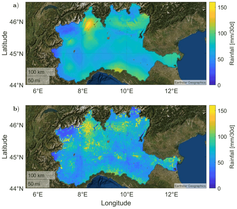
Figure 2Estimated average 30 d accumulated rainfall from the parameterized SM2RAIN applied to ASCAT (a) and S1-RT1 (b) SM product for the period 2016–2019. Map copyright © 2021 GeoBasis-De/BKG (© 2009), Google, Inst. Geogr. Nacional Immagini © 2021 TerraMetrics.
The results of R, RMSE and bias with respect to the selected time steps are shown in Fig. 3. In order to maximize the reliability of the obtained performances, the rainfall accumulation was carried out by summing up only timestamps available in both the SM2RAIN estimations and the benchmark, for each SM2RAIN product separately. In this way S1-RT1 performances can be better assessed, since a direct accumulation would penalize this product due to the long period of no data caused by S1 low temporal resolution.

Figure 3Violin plots of Pearson's correlation (R, a), root mean square error (RMSE, b) and bias (c) between the rainfall from MCM and from SM2RAIN applied to ASCAT and S1-RT1. ASCAT-derived rainfall was accumulated at 1, 10 and 30 d, while the rainfall from S1-RT1 was accumulated at 10 and 30 d. Each violin shape is obtained by rotating a smoothed kernel density estimator. The green violins are obtained by calibrating SM2RAIN against MCM, while the red violins are derived from the parameterized SM2RAIN procedure.
The SM2RAIN product obtained from ASCAT allows us to reproduce the rainfall of the Po River basin well at daily timescale, thanks to the high temporal resolution of ASCAT (sub-daily frequency), with a median R of 0.61 for the parameterized product and 0.64 for the calibrated product, confirming the good quality of the data and the importance of its temporal resolution. At higher aggregation time steps, the median R of the parameterized (calibrated) ASCAT-derived rainfall products improves to 0.71 (0.75) for the 10 d accumulation period and to 0.74 (0.77) when 30 d accumulation is considered. Good results are also obtained from the application of SM2RAIN to S1-RT1, with a median R of 0.61 (0.65) and 0.73 (0.75) at 10 and 30 d accumulation time, respectively. Apart from ASCAT-derived rainfall performing better than the one from S1-RT1 at 10 d, they are equally good for the 30 d accumulated rainfall. The results also confirm the good capabilities of the parameterized SM2RAIN algorithm in rainfall estimation, considering the small differences between the performances obtained by the two algorithm versions. The only exception is the bias index, which, as expected, is significantly larger in the parameterized products compared to the calibrated ones. The increased bias is due to the ERA5-Land data used to obtain the climatology of the area since its spatial resolution is much lower than the one adopted for this study (i.e., 1 km), and the average spatial pattern of rainfall is quite different from the one measured by MCM.
4.2 Spatial validation of rainfall products
Even if the ASCAT product (with lower spatial resolution) is on average the best-performing, the spatial comparison of the performances is important to understand the added value of high-resolution SM. In order to better evaluate the differences between the rainfall estimated from ASCAT and S1-RT1, Pearson's correlation performances of the 30 d accumulated rainfall derived from the two SM products are analyzed in this section. This temporal step was selected since it is suited for a quality comparison of the two products, being less influenced by the different temporal resolution of the sensors and because it is optimal for agricultural application.
Generally good performances are obtained from both rainfall products, as shown in Fig. 4a and b. Some areas with low R values are shared by both ASCAT- and S1-RT1-derived rainfall products. Over mountain areas, the errors are mostly related to the lower accuracy of C-band SM data, due to shadowing effects and layover (a distortion that occurs in radar imaging when the signal reflected from the top of a tall feature is received by the emitter before the one of the base; Ulaby et al., 1981). The presence of water bodies at the river outlet and over the paddy fields in the western part of the Po basin also affects SM and hence rainfall retrieval accuracy. Finally, the yellow “holes” in the correlation maps resemble the errors caused by low-quality gauge data, which affect the rainfall estimation surrounding the gauge sensor. It should also be noticed that many low-performing areas are located close to urban centers, which may affect both the SM retrieval quality and the rain gauge measurements, as discussed in the following section. Notwithstanding this, it is impossible to remove the alleged “bad” gauge stations from the benchmark product, as MCM is an operative product, and the clear identification of these stations is often challenging.
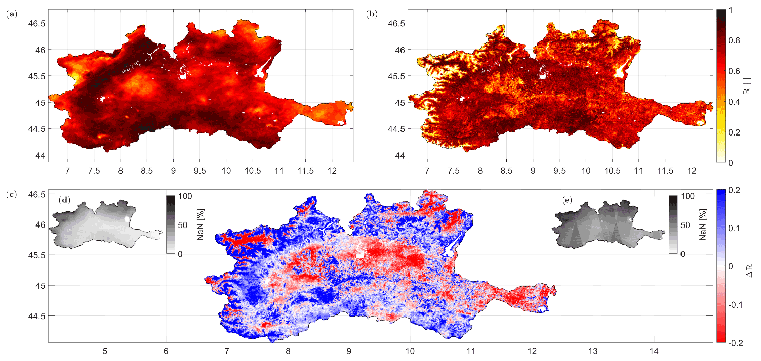
Figure 4Spatial Pearson's correlation (R) between the 30 d accumulated rainfall derived from MCM and the application of the parameterized SM2RAIN to ASCAT (a) and to S1-RT1 (b) SM products. Panel (c) shows the difference between ASCAT and S1-RT1 correlation maps, while panels (d) and (e) show the percentage of invalid images per pixel respectively for ASCAT and S1-RT1.
The spatial comparison between the performances of the ASCAT- and S1-RT1- derived rainfall is shown in Fig. 4c, displaying the difference between the correlation values of the two products. Red areas mean that the S1-RT1 product is performing better, whereas blue areas highlight where ASCAT is providing more accurate rainfall estimates. First of all, it should be noted that while the ASCAT-derived rainfall product shows average correlation values over the mountainous region in the north and west of the map (see Fig. 1 for comparison with the DEM map), S1-RT1 correlation is either extremely low or extremely high. This important difference is caused by the high spatial resolution of the S1-RT1 product: the improved resolution allows the “good” signal originating from the valleys to be clearly distinguished from the “bad” signal coming from the mountain slopes, affected by the noise generated from the aforementioned shadowing and layover effects. This distinction results in areas with very good (valleys) and very bad (mountains) rainfall estimations. The spatial resolution of ASCAT on the other hand does not allow the signals of the two geographical features to be distinguished, causing lower performances over the valleys and higher performances over the slopes in comparison with S1-RT1. The low performances of the pixels located over the mountain slopes are also responsible for the long violin plot tails of S1-RT1 performances that can be noticed in Fig. 3. S1-RT1 results are particularly lower than those from ASCAT due to the fact that S1-RT1 product calibration was carried out without considering any snow masking, thus reducing the quality of the solution in the pixels affected by snow cover.
A smaller difference in performance can be noticed over the plain, in particular in the northeastern section, where S1-RT1 rainfall performs overall better than ASCAT. Conversely, in the southern section and specifically over the areas surrounding the Po River and its tributaries, ASCAT-derived rainfall is better than S1. An explanation of this behavior can be found in the intensive irrigation practice over this area. Irrigation events cause an increase of the fields SM (Filippucci et al., 2020) that should be sensed by satellite sensors. However, the area surrounding the Po River is composed by many small fields (a few hectares each) managed by different farmers, where the irrigation timing is not concurrent. The ASCAT sensor is not able to distinguish the resulting irrigation signal (Brocca et al., 2018) because of its low spatial resolution (25 km) that cause the signals of each field to overlap and average with each other. S1, instead, is more sensitive to the irrigation signal, thanks to its higher spatial resolution.
Considering that the rainfall benchmark product does not contain irrigation information, the drop in Pearson's correlation of the S1-RT1-derived rainfall with respect to ASCAT could be related to the sensitiveness of the former to the aforementioned irrigation events and not to the SM signal quality. It could be an additional information of great scientific interest, but, unfortunately, the absence of detailed irrigation data for the Po Valley makes it difficult to verify this hypothesis.
Finally, it should also be noted that this analysis could be biased in the areas characterized by a high presence of missing values (NaN) for one product with respect to the other, which hampers the statistical significance of the performance indices. Notwithstanding this, the absence of patterns in the maps that resemble the NaN distribution percentage shown in Fig. 4d and e fosters the validity of the analysis, even if S1 temporal resolution still affects the average rainfall pattern (compare Fig. 4e with 2b).
The performance comparison with respect to RMSE and bias and a comparison of the calibrated SM2RAIN products is omitted for the sake of brevity because no relevant additional information can be obtained from it.
In Figs. 5 and 6, rainfall and SM time series of two pixels selected in the northwest of the Po basin are shown, as an example of the increased capacity of S1-RT1 for rainfall retrieval in the mountainous area. Since these pixels are selected in a topographic complex area, they should not be considered representatives of the overall performance and availability of the satellite rainfall products, rather an example of the improved performance derived from the use of S1-RT1 high-resolution SM. Winter and early-spring measurements are masked in both pixels, due to frozen conditions or snow cover, according to ERA5-Land information. The pixel in Fig. 5 is selected over one of the mountain valleys of the Italian territory (7.152∘ E, 45.710∘ N), inside the Italian region Valle d'Aosta, in order to show how S1 spatial resolution increases the capabilities in rainfall estimation over such a region. By observing the rainfall time series in Fig. 5a and the standard month distribution in Fig. 5b, it can be noted how S1-RT1-derived rainfall is in better accordance with the observed one, in particular during autumn months. During late spring and summer, S1-RT1 and ASCAT estimates are more similar, while S1-RT1 often underestimates the observed rainfall, also with respect to ASCAT. In Fig. 5d, the same behavior can be noted on the averaged SM trends, with the SM sensed by S1-RT1 being on average less than the one from ASCAT during late spring–summer and greater during the autumn season, probably due to the additional vegetation correction operated within S1-RT1.
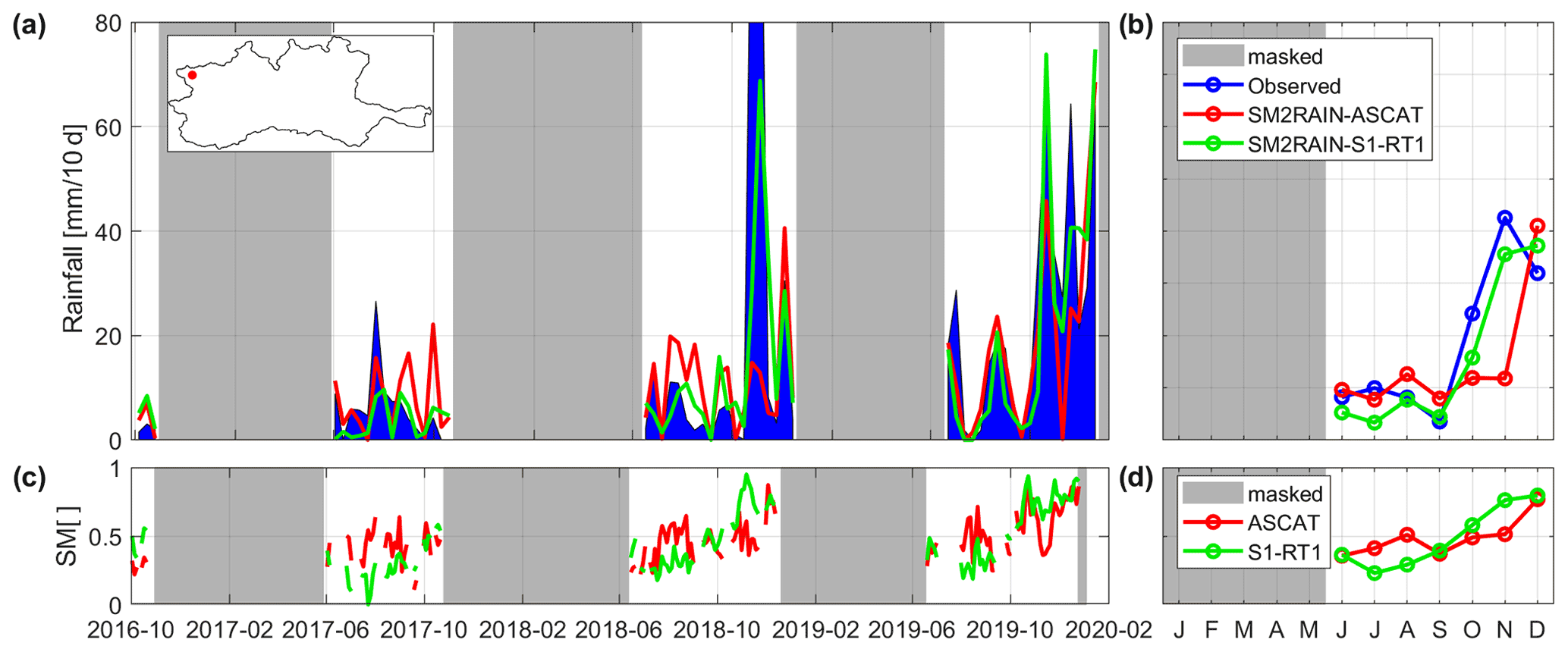
Figure 5Example of SM and rainfall time series over a pixel (7.152∘ E, 45.710∘ N) where the parameterized SM2RAIN applied to S1-RT1 outperforms SM2RAIN-ASCAT. In (a), the time series of the observed (blue) and estimated (red SM2RAIN-ASCAT, green SM2RAIN-S1-RT1) 10 d accumulated rainfall products are shown, while panel (c) displays SM time series averaged with a 3 d window. Finally, panels (b) and (d) contain the standard month average of the rainfall and SM products, respectively. The periods masked for frozen soil conditions or snow cover are highlighted in grey.

Figure 6Example of SM and rainfall time series over a pixel (7.410∘ E, 45.824∘ N) where the parameterized SM2RAIN-ASCAT outperforms SM2RAIN applied to S1-RT1. In (a), the time series of the observed (blue) and estimated (red SM2RAIN-ASCAT, green SM2RAIN-S1-RT1) 10 d accumulated rainfall products are shown, while panel (c) displays SM time series averaged with a 3 d window. Finally, panels (b) and (d) contain the standard month average of the rainfall and SM products, respectively. The periods masked for frozen soil conditions or snow cover are highlighted in grey.
Figure 6 shows the time series of a pixel selected over the mountain slopes, in the vicinity of the previous one (7.410∘ E, 45.824∘ N). While ASCAT SM estimates (Fig. 6c and d) show patterns that are similar to those in Fig. 5, the S1-RT1 signal is completely different. The SM saturates in the summer period and goes down in autumn, with a strong seasonality that is poorly affected by the rainfall events. This is most probably an issue of the vegetation correction, since it adds a strong seasonality to pixels that realistically exhibit little vegetation coverage, also due to the low spatial resolution (with respect to S1-RT1) of the LAI product used for correcting vegetation seasonalities. This erroneous vegetation seasonality is then counteracted by an erroneous SM seasonality. As expected, the poor quality of SM estimations greatly affects SM2RAIN capabilities in calculating rainfall in these areas, resulting in a very high rainfall rate perceived during summer and a very low one during winter, in contrast with the observed data.
Finally, Fig. 7 shows the time series of a pixel selected over the plain (10.684∘ E, 44.805∘ N). As can be noted, the period of unavailability of the rainfall datum is greatly reduced in comparison with Figs. 5 and 6, since this area is characterized by higher temperature during the winter and by minor snow cover probability. Overall, S1-RT1 SM shows a greater variability during the summer season with respect to ASCAT (Fig. 7c, d), thanks to both the vegetation correction and the higher spatial resolution. This leads to a greater accuracy in the peak rainfall detection of summer 2018 and 2019 (Fig. 7a). On the other hand, an overestimation of 2017 summer rainfall (potentially due to an error in SM estimation or to an irrigation event) and an underestimation of winter 2019 (probably due to SM saturation) are found. Overall, the rainfall estimate from S1-RT1 is in good accordance with the observed one (Fig. 7b), proving both the validity of the derived rainfall product and its usefulness for hydrologic modeling.
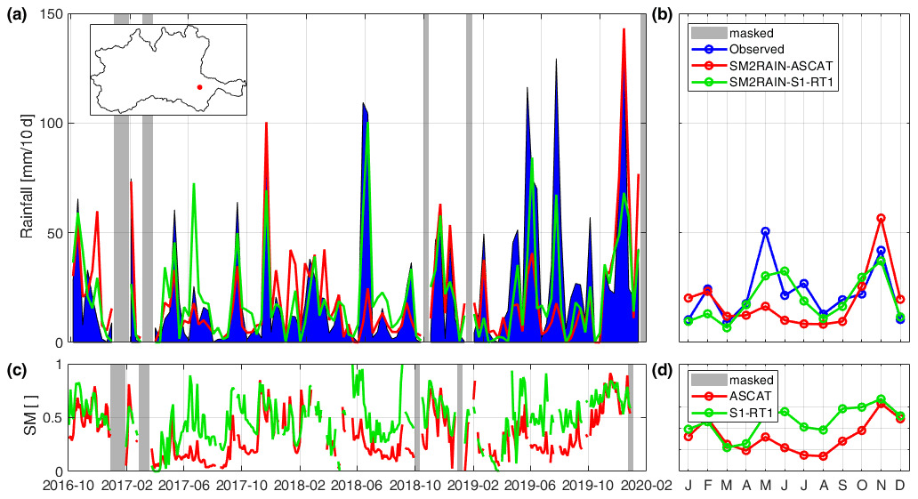
Figure 7Example of SM and rainfall time series over a pixel (10.684∘ E 44.805∘ N) selected in the plain. In (a), the time series of the observed (blue) and estimated (red SM2RAIN-ASCAT, green SM2RAIN-S1-RT1) 10 d accumulated rainfall products are shown, while panel (c) displays SM time series averaged with a 3 d window. Finally, panels (b) and (d) contain the standard month average of the rainfall and SM products, respectively. The periods masked for frozen soil conditions or snow cover are highlighted in grey.
The obtained results show that the high-resolution information from S1 sensors allows the accuracy of SM (and thus of rainfall) to be increased in areas where coarse-resolution data are not able to obtain reliable estimates. Conversely, over some regions, the rainfall obtained from the application of SM2RAIN to S1-RT1 SM shows worse performance with respect to the one obtained when the algorithm is applied to ASCAT data, as is the case over many mountainous areas. Finally, the analysis highlighted some areas in which the accuracy of the rainfall obtained from the application of both the calibrated and parameterized SM2RAIN to ASCAT or S1-RT1 SM products is stably low, as discussed in Sect. 4.2. This issue can depend on multiple factors, such as SM signal quality, failure of the SM2RAIN algorithm hypothesis or accuracy of the benchmark rainfall product. An attempt to identify these areas is made here, by highlighting the pixels in which Pearson's correlation between the 30 d accumulated rainfall from MCM and the four SM2RAIN-derived products is always less than a threshold, fixed at 0.65, as shown in Fig. 8. Multiple areas of stable low performances can be distinguished in the figure, highlighted in blue. Two main reasons for this behavior can be identified: issues with the SM sensing and issues with the benchmark product.
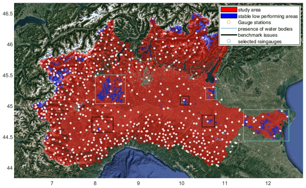
Figure 8Map of Po River basin. The blue pixels indicate the areas where Pearson's correlation between the 30 d accumulated rainfall from MCM and the calibrated and parameterized SM2RAIN applied to ASCAT or S1-RT1 is stably less than a threshold of 0.65. The light blue rectangles surround the areas with paddy areas or abundant water bodies, while black rectangles outline areas with alleged “bad”-performing gauge stations. Finally, the white dots show the gauge station locations and the green dots the rain gauge selected to be analyzed further. Map copyright © 2021 GeoBasis-De/BKG (© 2009), Google, Inst. Geogr. Nacional Immagini © 2021 TerraMetrics.
In particular, the blue areas located in mountainous region in Fig. 8, in the north and the west of the map, should be affected by both the source of error, since in topographically complex areas, SM retrieval is difficult, and weather radar accuracy drops. Notwithstanding this, ASCAT performance is still higher than that of S1-RT1 in these areas (compare with Fig. 4). This fact has a threefold explanation: first, S1-RT1 SM estimations are obtained without considering any snow masking; thus their accuracy over mountain region regularly affected by snow cover is limited. Second, the low quality of ASCAT SM retrieval over topographically complex areas is mitigated by the presence of valleys and/or a plateau in each ASCAT pixel in which SM accuracy is higher. Third, the SM2RAIN algorithm hypothesis could be invalid over these areas since the runoff rate should be not negligible. Indeed, SM2RAIN conditions state that the runoff rate is negligible during the rainfall event, but the low temporal resolution of S1 overcomes the duration of most of the events, questioning the condition's validity.
Instead, the areas in Fig. 8 within the light blue rectangles are characterized by the presence of paddies and water bodies: here the low performance should be caused by low SM quality, due to the impossibility of retrieve SM information over flooded areas with active microwave sensors. Finally, the remaining blue regions should be affected by low quality of the benchmark product. This can be related either to “bad”-performing gauge stations, recognizable through the central position of a gauge with respect to the low-performing area (e.g., the two regions in the center–east black rectangles), or to issues with weather radar and rain gauge measurements, where the blue patterns are concentrated between two or more rain gauges (e.g., the region within the black rectangles in the southwest).
In order to better analyze this aspect, three stations located within the three black rectangles in Fig. 8 were selected, together with the nearest-neighbor stations. The MCM time series of the pixels that include the stations were extracted, in order to compare them and assess the quality of the selected rain gauges. The qualitative comparison of the stations is shown in Fig. 9, where the scatter plots for each pair of rain gauges are shown, together with their position in the map (Fig. 9a). In particular, a clear issue with the rain gauge named A1 can be appreciated in Fig. 9b, with this sensor measuring rainfall peaks up to 300 mm d−1, absent from the nearest gauges. The issue can be confirmed by the low Pearson correlation between its time series and the one of the nearest rain gauge, equal to 0.53, that is significantly lower than the mean Pearson correlation calculated between each couple of nearest stations within the study area, equal to 0.87 (standard deviation equal to 0.1). Also, Fig. 9c shows strange patterns of rainfall: even if there are no large peaks, several rainfall events are sensed with different magnitude by the two stations named B1 and B2, as can be noticed by looking at the number of points that tends to the x and y axis which indicate severe over- or underestimation. Also in this case, the measured Pearson correlation is lower than the average, equal to 0.71. Finally, station C1 (Fig. 9d) measures several peaks of rainfall that are higher than those recorded by the nearest rain gauge, C2. Notwithstanding this, in this case, the variation between the two sensors seems to be caused by the natural rainfall spatial variability, as demonstrated by the high Pearson correlation between the two time series, equal to 0.88. This was expected since the low-performing region is not located around one of the stations but in between them, over a hilly area that could affect the weather radar measurements.

Figure 9Panel (a) shows the boundary of the Po River basin, together with the position of three couple of stations (A1–A2, B1–B2 and C1–C2) with alleged “bad” MCM performance. The scatter plots of the daily rainfall measured by each couple of stations are then shown in (b), (c) and (d).
Errors in the selected benchmark product are a known limitation of the direct validation of rainfall datasets. This fact is also the proof of the need of further research in the rainfall measurement fields, since the merging of different rainfall products, each with its limitation often complementary, can be beneficial, allowing a more reliable estimate to be obtained.
Rainfall measurements from space are more and more used to increase the rainfall distribution knowledge and to improve water resource management capabilities, but their spatial resolution is limited due to technological limitations. In this work, the SM2RAIN algorithm was applied to a 1 km spatial resolution SM product from S1 obtained through an algorithm based on a first-order solution of the Radiative Transfer equation, RT1, over the Italian fraction of the Po River basin (Fig. 1), to obtain a high-resolution rainfall product from satellite remote sensing. This region was selected due to the availability of a benchmark dataset from radar and rain gauge data, obtained through the MCM algorithm. Two versions of SM2RAIN were applied in this analysis to compare the resulting performances: one uncalibrated, to foster the high-resolution rainfall estimation in other regions where benchmark data are unavailable, and one calibrated against the observed data. In order to assess the improvements related to the high spatial resolution of S1, SM2RAIN was also applied to ASCAT SM, resampled to S1-RT1 grid for comparison. The analysis was carried out at different temporal accumulation steps (1, 10 and 30 d) to take the different temporal resolutions of the two SM products, 1.5 to 4 d for S1-RT1 and sub-daily for ASCAT, into account.
The results (Fig. 3) show that it is indeed possible to obtain high-resolution rainfall data from S1, even if the low temporal resolution of the data does not allow daily rainfall to be calculated. It is instead possible to calculate it with ASCAT data due to the higher temporal resolution, with good results (median R of 0.61 and 0.64 for the parameterized and calibrated SM2RAIN). When 10 d accumulated rainfall is considered, S1-RT1-derived rainfall from the parameterized (calibrated) SM2RAIN performs quite well, with a median R of 0.61 (0.65), but ASCAT performances are higher, with a median R of 0.71 (0.75). At higher temporal accumulation steps, the performance differences reduce, until ASCAT- and S1-RT1-derived rainfall reach almost equal R for the 30 d accumulated rainfall (around 0.75). A similar conclusion can be deduced by analyzing the RMSE index, while for the bias index the differences between the calibrated and the parameterized SM2RAIN results are larger, probably due to the low spatial resolution of the product used to obtain the Po River basin climatology (ERA5-Land).
Even if on average the rainfall from ASCAT seems to be slightly better-performing than the one from S1, the analysis of the spatial distribution of R shows instead the true benefits of the high-resolution SM (Fig. 4). In complex mountain regions, S1 obtains extremely good performance over the valleys and bad performance over the ridges, unsuited for SM remote sensing, whereas ASCAT R always represents an average of the two signals due to the lower spatial resolution. S1-derived rainfall is generally better-performing than the one from ASCAT, also in the northern section of the Po Valley plain, while the latter is better in the southern section, where irrigation is widely practiced. The fragmentary nature of the irrigation in this area could be the cause of this phenomenon: S1-RT1 should be more sensitive than ASCAT to the signal generated by various small fields, where irrigation in not concurrent, thanks to its higher spatial resolution, but since irrigation is not considered in the benchmark product, the resulting R is reduced.
Some areas with stable low performance of rainfall estimation were also identified (Fig. 8), caused by the limitations of SM2RAIN algorithm (e.g., areas in which runoff rate is not negligible), of the SM remote sensing (areas in which SM estimation is impossible, e.g., flooded or snow-covered areas) and of the benchmark product (e.g., topographically complex areas).
Summing up, high-resolution rainfall from satellite remote sensing is possible and is able to observe features that are averaged in products with lower spatial resolution, like the precipitation within mountain valleys and potentially the fields' irrigation. Notwithstanding this, the low temporal resolution is currently a limitation for its application in many fields, even if high-spatial-resolution rainfall at monthly temporal resolution is still useful for agriculture, water resource management and index-based insurances. Future research steps should try to address this issue, e.g., by exploiting the integration of high-spatial-resolution products (characterized by low frequency) with high-temporal-resolution products (characterized by low spatial resolution).
In this paper, the performance indexes were calculated at three different temporal steps: 1, 10 and 30 d. In order to obtain them, the time series of each estimated product and the observed one were accumulated according to the selected period by considering only the intervals in which the data were available in both the datasets. This choice was made to obtain the best accurate assessment of each product, by calculating its potential in estimating rainfall against a concurrent dataset. Notwithstanding this, the comparison of ASCAT and S1-RT1 based on such performances could be biased because in this way the analyzed indexes are calculated against two different benchmark datasets, each representing only the selected overlapping timestamps. In this section, we decided therefore to calculate the performance indexes again by accumulating the rainfall of the observed and estimated datasets only over the periods in which the three datasets (i.e., MCM, ASCAT and S1-RT1) are available together and to insert in this appendix the corresponding figures with respect to the newly calculated indexes: Figs. 4 (A1) and 5 (A2). To further increase the comparison quality and to avoid the period in which just one Sentinel-1 sensor was in orbit and thus the associated drop in performance, only the data subsequent to 1 October 2016 were considered for the new index calculation.
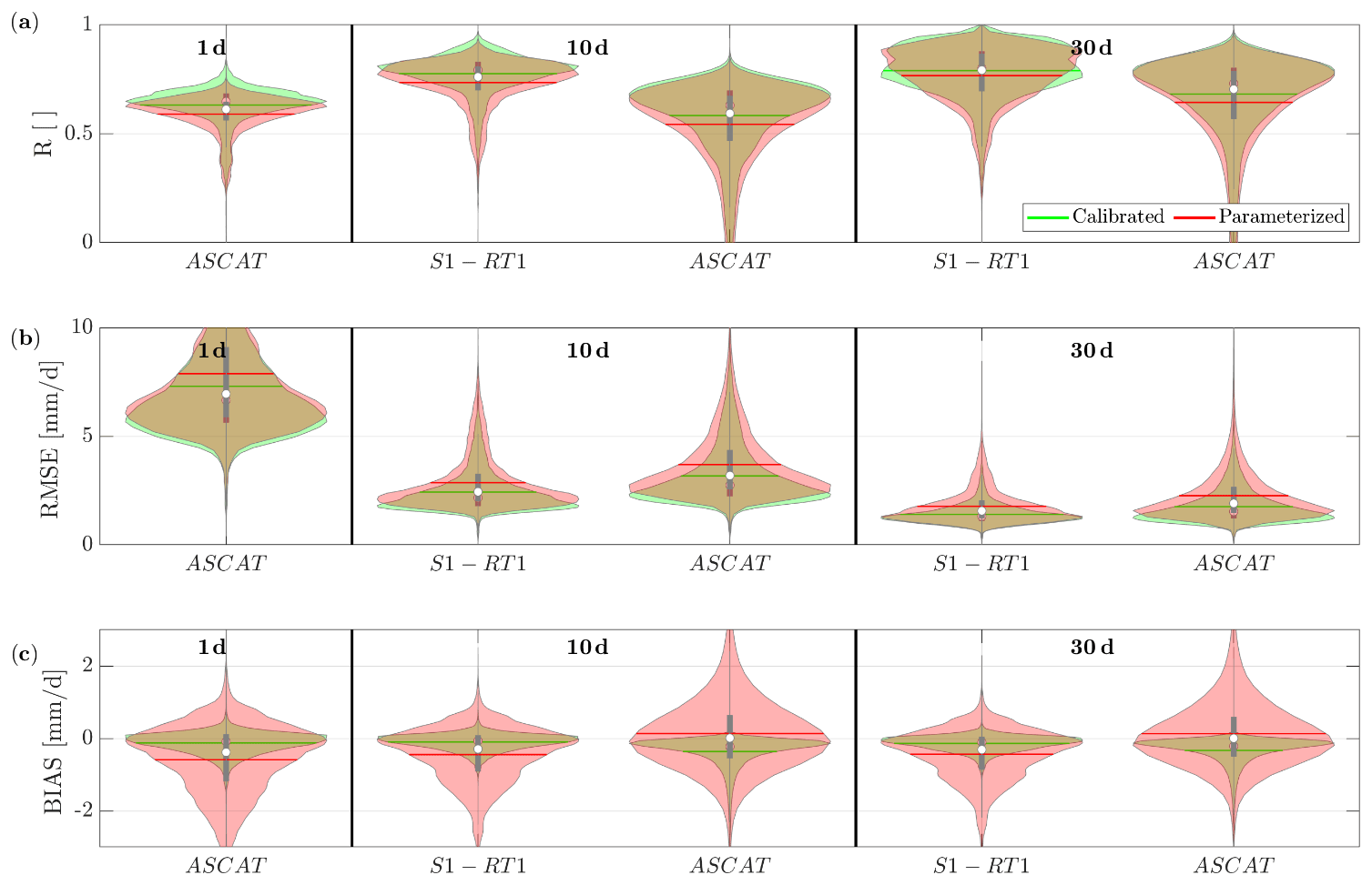
Figure A1Violin plots of Pearson's correlation (R, a), root mean square error (RMSE, b) and bias (c) between the rainfall from MCM and from SM2RAIN applied to ASCAT and S1-RT1. ASCAT-derived rainfall was accumulated at 1, 10 and 30 d, while the rainfall from S1-RT1 was accumulated at 10 and 30 d. Only the periods in which all three products are available are considered in the accumulation. Each violin shape is obtained by rotating a smoothed kernel density estimator. The green violins are obtained by calibrating SM2RAIN against MCM, while the red violins are derived from the parameterized SM2RAIN procedure.
In comparison with the paper's results, here ASCAT performances increase, evidently due to the removal of some low-performing data, as confirmed by the appearance of some patterns within the ASCAT correlation maps in Fig. A2a that resemble the invalid pixel percentage distributions map of Fig. A2d. Notwithstanding this, the areas in which S1-RT1 outperforms ASCAT are almost identical, although shrunk, confirming the paper's results.
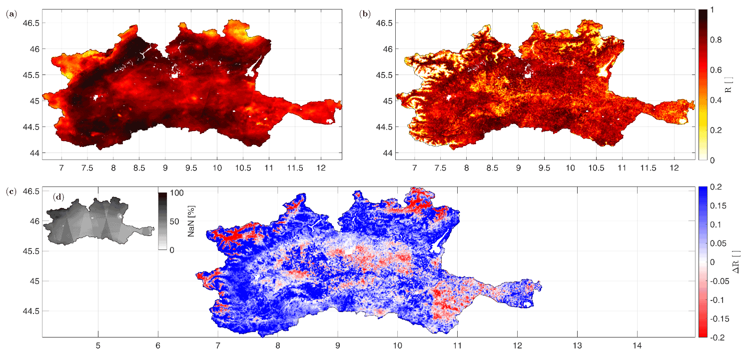
Figure A2Spatial Pearson's correlation (R) between the 30 d accumulated rainfall derived from MCM and the application of the parameterized SM2RAIN to ASCAT (a) and to S1-RT1 (b) SM products, only considering the periods for which all three products are available. Panel (c) shows the difference between ASCAT and S1-RT1 correlation maps, while panel (d) shows the percentage of invalid images per pixel.
The code of the SM2RAIN algorithm is available at https://doi.org/10.5281/zenodo.2203559 (Hahn, 2018), while the rainfall data obtained in this work can be downloaded from https://doi.org/10.5281/zenodo.6530709 (Filippucci et al., 2022). The topographic data were downloaded and are available from the NASA Earthdata data repository. The local observations were obtained from the National Department of Civil Protection and cannot be shared with third parties.
PF and LB designed the experiment. LB obtained the funds. PF, RQ and LC gathered and managed the data. PF was is charge of the formal analysis, investigation, methodology, project administration, software, validation and visualization, while LB, CS, WW and AT supervised the work. PF prepared the manuscript with contributions from the coauthors. All the coauthors contributed to the review and editing of the manuscript.
The contact author has declared that neither they nor their co-authors have any competing interests.
Publisher’s note: Copernicus Publications remains neutral with regard to jurisdictional claims in published maps and institutional affiliations.
The support of the CIMA Foundation in providing the high-resolution rainfall dataset is gratefully acknowledged.
This research has been supported by the Österreichische Forschungsförderungsgesellschaft (DWC Radar project, grant no. CNR-IRPI 24840/2019), the European Organization for the Exploitation of Meteorological Satellites (H SAF project, grant no. EUM/C/85/16/LOD and EUM/C/85/16/MIN) and the European Space Agency (DTE Hydrology project, grant no. ESA 4000129870/20/I-NB (CCN N. 1)).
This paper was edited by Rohini Kumar and reviewed by two anonymous referees.
Albergel, C., Rüdiger, C., Pellarin, T., Calvet, J.-C., Fritz, N., Froissard, F., Suquia, D., Petitpa, A., Piguet, B., and Martin, E.: From near-surface to root-zone soil moisture using an exponential filter: an assessment of the method based on in-situ observations and model simulations, Hydrol. Earth Syst. Sci., 12, 1323–1337, https://doi.org/10.5194/hess-12-1323-2008, 2008.
Barrett, E. C. and Beaumont, M. J.: Satellite rainfall monitoring: An overview, Remote Sensing Reviews, 11, 23–48, https://doi.org/10.1080/02757259409532257, 1994.
Bauer-Marschallinger, B., Paulik, C., Hochstöger, S., Mistelbaue, T., Modanesi, S., Ciabatta, L., Massari, C., Brocca, L., and Wagner, W.: Soil Moisture from Fusion of Scatterometer and SAR: Closing the Scale Gap with Temporal Filtering, Remote Sens., 10, 1030, https://doi.org/10.3390/rs10071030, 2018.
Bauer-Marschallinger, B., Cao, S., Navacchi, C., Freeman, V., Reuß, F., Geudtner, D., Rommen, B., Vega, F. C., Snoeij, P., Attema, P., Reimer, C., and Wagner W.: The normalised Sentinel-1 Global Backscatter Model, mapping Earth’s land surface with C-band microwaves, Scientific Data, 8, 277, https://doi.org/10.1038/s41597-021-01059-7, 2021.
Black, E., Tarnavsky, E., Maidment, R., Greatrex, H., Mookerjee, A., Quaife, T., and Brown, M.: The Use of Remotely Sensed Rainfall for Managing Drought Risk: A Case Study of Weather Index Insurance in Zambia, Remote Sens., 8, 342, https://doi.org/10.3390/rs8040342, 2016.
Brocca, L., Melone, F., Moramarco, T., and Wagner, W.: A new method for rainfall estimation through soil moisture observations, Geophys. Res. Lett., 40, 853–858, https://doi.org/10.1002/grl.50173, 2013.
Brocca, L., Ciabatta, L., Massari, C., Moramarco, T., Hahn, S., Hasenauer, S., Kidd, R., Dorigo, W., Wagner, W., and Levizzani, V.: Soil as a natural rain gauge: estimating global rainfall from satellite soil moisture data, J. Geophsy. Res., 119, 5128–5141, https://doi.org/10.1002/2014JD021489, 2014.
Brocca, L., Massari, C., Ciabatta, L., Moramarco, T., Penna, D., Zucco, G., Pianezzola, L., Borga, M., Matgen, P., and Martínez-Fernández, J.: Rainfall estimation from in situ soil moisture observations at several sites in Europe: an evaluation of SM2RAIN algorithm, J. Hydrol. Hydromech., 63, 201–209, https://doi.org/10.1515/johh-2015-0016, 2015.
Brocca, L., Tarpanelli, A., Filippucci, P., Dorigo, W., Zaussinger, F., Gruber, A., and Fernàndez-Prieto, D.: How much water is used for irrigation? A new approach exploiting coarse resolution satellite soil moisture products, Int. J. Appl. Earth Obs., 73, 752–766, https://doi.org/10.1016/j.jag.2018.08.023, 2018.
Brocca, L., Filippucci, P., Hahn, S., Ciabatta, L., Massari, C., Camici, S., Schüller, L., Bojkov, B., and Wagner, W.: SM2RAIN–ASCAT (2007–2018): global daily satellite rainfall data from ASCAT soil moisture observations, Earth Syst. Sci. Data, 11, 1583–1601, https://doi.org/10.5194/essd-11-1583-2019, 2019.
Bruno, G., Pignone, F., Silvestro, F., Gabellani, S., Schiavi, F., Rebora, N., Giordano P., and Falzacappa, M.: Performing Hydrological Monitoring at a National Scale by Exploiting Rain-Gauge and Radar Networks: The Italian Case, Atmosphere, 12, 771, https://doi.org/10.3390/atmos12060771, 2021.
Ciabatta, L., Massari, C., Brocca, L., Gruber, A., Reimer, C., Hahn, S., Paulik, C., Dorigo, W., Kidd, R., and Wagner, W.: SM2RAIN-CCI: a new global long-term rainfall data set derived from ESA CCI soil moisture, Earth Syst. Sci. Data, 10, 267–280, https://doi.org/10.5194/essd-10-267-2018, 2018.
Crow, W. T., Huffman, G. F., Bindlish, R., and Jackson, T. J.: Improving satellite rainfall accumulation estimates using spaceborne soil moisture retrievals, J. Hydrometeorol., 10, 199–212, https://doi.org/10.1175/2008JHM986.1, 2009.
Crow, W. T., van den Berg, M. J., Huffman, G. J., and Pellarin, T.: Correcting rainfall using satellite-based surface soil moisture retrievals: The Soil Moisture Analysis Rainfall Tool (SMART), Water Resour. Res., 47, W08521, https://doi.org/10.1029/2011WR010576, 2011.
Dari, J., Brocca, L., Quintana-Seguí, P., Escorihuela, M. J., Stefan, V., and Morbidelli, R.: Exploiting High-Resolution Remote Sensing Soil Moisture to Estimate Irrigation Water Amounts over a Mediterranean Region, Remote Sens., 12, 2593, https://doi.org/10.3390/rs12162593, 2020.
Dinku, T.: Challenges with availability and quality of climate data in Africa, in: Extreme Hydrology and Climate Variability, edited by: Melesse, A., Abtew, W., and Senay, G., Elsevier, 71–80, ISBN 9780128159989, https://doi.org/10.1016/B978-0-12-815998-9.00007-5, 2019.
Enenkel, M., Osgood, D., Anderson, M., Powell, B., McCarty, J., Neigh, C., Carroll, M., Wooten, M., Husak, G., Hain, C., and Brown, M.: Exploiting the Convergence of Evidence in Satellite Data for Advanced Weather Index Insurance Design, Weather Clim. Soc., 11, 65–93, https://doi.org/10.1175/WCAS-D-17-0111.1, 2019.
Famiglietti, J. and Wood, E. F.: Multiscale modeling of spatially variable water and energy balance processes, Water Resour. Res., 30, 3061–3078, https://doi.org/10.1029/94WR01498, 1994.
Filippucci, P., Tarpanelli, A., Massari, C., Serafini, A., Strati, V., Alberi, M., Raptis, K. G. C., Mantovani, F., and Brocca, L.: Soil moisture as a potential variable for tracking and quantifying irrigation: A case study with proximal gamma-ray spectroscopy data, Adv. Water Resour., 136, 103502, https://doi.org/10.1016/j.advwatres.2019.103502, 2020.
Filippucci, P., Brocca, L., Massari, C., Saltalippi, C., Wagner, W., and Tarpanelli, A.: Toward a self-calibrated and independent SM2RAIN rainfall product, J. Hydrol., 603, 126837, https://doi.org/10.1016/j.jhydrol.2021.126837, 2021.
Filippucci, P., Brocca, L., Quast, R., Ciabatta, L., Saltalippi, C., Wagner, W., and Tarpanelli, A.: High resolution (1 km) satellite rainfall estimation from SM2RAIN applied to Sentinel-1: Po River Basin as case study, Hydrology and Earth System Sciences, Zenodo [data set], https://doi.org/10.5281/zenodo.6530709, 2022.
Hahn, S.: IRPIhydrology/sm2rain: SM2RAIN (v0.0.1), Zenodo [code], https://doi.org/10.5281/zenodo.2203559, 2018.
Hersbach, H., Bell, B., Berrisford, P., Hirahara, S., Horányi, A., Muñoz-Sabater, J., Nicolas, J., Peubey, C., Radu, R., Schepers, D., Simmons, A., Soci, C., Abdalla, S., Abellan, X., Balsamo, G., Bechtold, P., Biavati, G., Bidlot, J., Bonavita, M., De Chiara, G., Dahlgren, P., Dee, D., Diamantakis, M., Dragani, R., Flemming, J., Forbes, R., Fuentes, M., Geer, A., Haimberger, L., Healy, S., Hogan, R. J., Hólm, E., Janisková, M., Keeley, S., Laloyaux, P., Lopez, P., Lupu, C., Radnoti, G., de Rosnay, P., Rozum, I., Vamborg, F., Villaume, S., and Thépaut, J. N.: The ERA5 global reanalysis, Q. J. Roy. Meteor. Soc., 146, 1999–2049, https://doi.org/10.1002/qj.3803, 2020.
Kidd, C. and Levizzani, V.: Status of satellite precipitation retrievals, Hydrol. Earth Syst. Sci., 15, 1109–1116, https://doi.org/10.5194/hess-15-1109-2011, 2011.
Kidd, C., Becker, A., Huffman, G. J., Muller, C. L., Joe, P., Skofronick-Jackson, G., and Kirschbaum, D. B.: So, How Much of the Earth's Surface is Covered by Rain Gauges?, B. Am. Meteorol. Soc., 98, 69–78, https://doi.org/10.1175/BAMS-D-14-00283.1, 2017.
Kummu, M., Guillaume, J., de Moel, H., Eisner, S., Flörke, M., Porkka, M., Siebert, S., Veldkamp T. I. E., and Ward, P. J.: The world's road to water scarcity: shortage and stress in the 20th century and pathways towards sustainability, Sci. Rep., 6, 38495, https://doi.org/10.1038/srep38495, 2016.
La Barbera, P., Lanza, L. G., and Stagi, L.: Tipping bucket mechanical errors and their influence on rainfall statistics and extremes, Water Sci. Technol., 45, 1–9, https://doi.org/10.2166/wst.2002.0020, 2002.
Massari, C., Brocca, L., Pellarin, T., Abramowitz, G., Filippucci, P., Ciabatta, L., Maggioni, V., Kerr, Y., and Fernandez Prieto, D.: A daily 25 km short-latency rainfall product for data-scarce regions based on the integration of the Global Precipitation Measurement mission rainfall and multiple-satellite soil moisture products, Hydrol. Earth Syst. Sci., 24, 2687–2710, https://doi.org/10.5194/hess-24-2687-2020, 2020.
Merlin, O., Chehbouni, A., Walker, J. P., Panciera, R., and Kerr, Y. H.: A simple method to disaggregate passive microwave-based soil moisture, IEEE T. Geosci. Remote Sens., 46, 786–796, https://doi.org/10.1109/TGRS.2007.914807, 2008.
Peel, M. C., Finlayson, B. L., and McMahon, T. A.: Updated world map of the Köppen-Geiger climate classification, Hydrol. Earth Syst. Sci., 11, 1633–1644, https://doi.org/10.5194/hess-11-1633-2007, 2007.
Pellarin, T., Louvet, S., Gruhier, C., Quantin, G., and Legout, C.: A simple and effective method for correcting soil moisture and precipitation estimates using AMSR-E measurements, Remote Sens. Environ., 136, 28–36, https://doi.org/10.1016/j.rse.2013.04.011, 2013.
Peng, J., Loew, A., Merlin, O., and Verhoest, N. E.: A review of spatial downscaling of satellite remotely sensed soil moisture, Rev. Geophys., 55, 341–366, https://doi.org/10.1002/2016RG000543, 2017,
Quast, R. and Wagner, W.: Analytical solution for first-order scattering in bistatic radiative transfer interaction problems of layered media, Appl. Opt., 55, 5379–5386, https://doi.org/10.1364/ao.55.005379, 2016.
Quast, R., Albergel, C., Calvet, J. C., and Wagner, W.: A Generic First-Order Radiative Transfer Modelling Approach for the Inversion of Soil and Vegetation Parameters from Scatterometer Observations, Remote Sens., 11, 285, https://doi.org/10.3390/rs11030285, 2019.
Quast, R., Wagner, W., Bauer-Marschallinger, B., and Vreugdenhil, M.: Soil moisture retrieval from Sentinel-1 using a first-order radiative transfer model – a case-study over the Po-Valley, in preparation, 2022.
Ragettli, S., Cortés, G., Mcphee, J., and Pellicciotti, F.: An evaluation of approaches for modelling hydrological processes in high-elevation, glacierized Andean watersheds, Hydrol. Process., 28, 5674–5695, https://doi.org/10.1002/hyp.10055, 2013.
Rockström, J., Falkenmark, M., Lannerstad, M., and Karlberg, L.: The planetary water drama: Dual task of feeding humanity and curbing climate change, Geophys. Res. Lett., 39, L15401, https://doi.org/10.1029/2012GL051688, 2012.
Silberstein, R. P.: Hydrological models are so good, do we still need data?, Environ. Modell. Softw., 21, 1340–1352, https://doi.org/10.1016/j.envsoft.2005.04.019, 2006.
Tarpanelli, A., Massari, C., Ciabatta, L., Filippucci, P., Amarnath, G., and Brocca, L.: Exploiting a constellation of satellite soil moisture sensors for accurate rainfall estimation, Adv. Water Resour., 108, 249–255, https://doi.org/10.1016/j.advwatres.2017.08.010, 2017.
Ulaby, F. T., Moore, R. K., and Fung, A. K.: Microwave Remote Sensing, Active and Passive, vol. 1, 2, 3, Artech House, ISBN-13: 978-0890061909, 978-0201107609, 978-0890061923, Addison-Wesley Publishing Company, 1981.
Villarini, G., Mandapaka, P. V., Krajewski, W. F., and Moore, R. J.: Rainfall and sampling uncertainties: A rain gauge perspective, J. Geophsy. Res., 113, D11102, https://doi.org/10.1029/2007JD009214, 2008.
Wagner, W., Lemoine, G., and Rott, H.: A method for estimating soil moisture from ERS scatterometer and soil data, Remote Sens. Environ., 70, 191–207, https://doi.org/10.1016/S0034-4257(99)00036-X, 1999.
Wagner, W., Hahn, S., Kidd, R., Melzer, T., Bartalis, Z., Hasenauer, S., Figa-Saldaña, J., de Rosnay, P., Jann, A., Schneider, S., Komma, J., Kubu, G., Brugger, K., Aubrecht, C., Züger, J., Gangkofner, U., Kienberger, S., Brocca, L., Wang, Y., Blöschl, G., Eitzinger, J., and Steinnocher, K.: The ASCAT soil moisture product: A review of its specifications, validation results, and emerging applications, Meteorol. Z., 22, 5–33, https://doi.org/10.1127/0941-2948/2013/0399, 2013.
Wanders, N., Pan, M., and Wood, E. F.: Correction of real-time satellite precipitation with multi-sensor satellite observations of land surface variables, Remote Sens. Environ., 160, 206–221, https://doi.org/10.1016/j.rse.2015.01.016, 2015.