Impact of spatial distribution information of rainfall in runoff simulation using deep learning method

Rainfall-runoff modeling is of great importance for flood forecast and water management. Hydrological modeling is the traditional and commonly used approach for rainfall-runoff modeling. In recent years, with the development of artificial intelligence technology, deep learning models, such as the long short-term memory (LSTM) model, are increasingly applied to rainfall-runoff modeling. However, current works do not consider the effect of rainfall spatial distribution information on the results. Focusing on 10 catchments from the Catchment Attributes and Meteorology for Large-Sample Studies (CAMELS) dataset, this study compared the performance of LSTM with different look-back windows (7, 15, 30, 180, 365 d) for future 1 d discharges and for future multi-day simulations (7, 15 d). Secondly, the differences between LSTMs as individual models trained independently in each catchment and LSTMs as regional models were also compared across 10 catchments. All models are driven by catchment mean rainfall data and spatially distributed rainfall data, respectively. The results demonstrate that regardless of whether LSTMs are trained independently in each catchment or trained as regional models, rainfall data with spatial information improves the performance of LSTMs compared to models driven by mean rainfall data. The LSTM as a regional model did not obtain better results than LSTM as an individual model in our study. However, we found that using spatially distributed rainfall data can reduce the difference between LSTM as a regional model and LSTM as an individual model. In summary, (a) adding information about the spatial distribution of the data is another way to improve the performance of LSTM where long-term rainfall records are absent, and (b) understanding and utilizing the spatial distribution information can help improve the performance of deep learning models in runoff simulations.

1 Introduction

Rainfall-runoff simulations are vital for watershed water resources management and risk analysis (Montanari, 2005; Neitsch et al., 2011). In addition, rainfall-runoff simulation plays an increasingly important role as a technical basis for hydrological forecasting due to the frequent occurrence of extreme hydrological events caused by climate change (Grayman, 2011; Panagoulia and Dimou, 1997). As the most widespread and essential tool for water science research, hydrological model plays a pivotal role in rainfall-runoff simulation (Krause et al., 2005; Sood and Smakhtin, 2015). The development of hydrological models cannot be separated from the continuous research on hydrological processes. It is on the basis of the continuous understanding of hydrological processes that hydrological researchers have enough theoretical basis for building models that describe the interrelationship between the various hydrological elements and can simulate the overall hydrological cycle. The development of hydrological models has gone through two main stages, namely lumped hydrological models and distributed hydrological models (Devia et al., 2015). For example, the Stanford model was the first lumped hydrological model with a solid theoretical basis (Crawford, 1966). In 1977, British, Danish, and French researchers jointly proposed the SHE (Systeme Hydrologique Europeen) hydrological model, which represents the first generation of distributed hydrological models (Sahoo et al., 2006). The variable infiltration capacity (VIC) model is a large-scale-distributed hydrological model developed by the University of Washington, the University of California at Berkeley, and Princeton University (Liang et al., 1996). The distributed VIC model is based on the idea of gridding to achieve distributed simulation of watersheds.

However, the fact that we cannot accurately describe every process of the hydrological cycle leads to the necessary simplifications in the hydrological model calculation process, which is one of the contributing factors to simulation errors. Since models based on physical mechanisms cannot fully describe the physical processes of the hydrological cycle, researchers started to explore data-driven models for hydrological modeling (Solomatine and Ostfeld, 2008). For example, support-vector machines (SVMs) are often used to manage the processing of hydrological model input data or to perform hydrological simulations directly due to their advantages in processing nonlinear problems (Ahmad et al., 2010; Sivapragasam et al., 2001). Artificial neural networks (ANNs) are a type of machine learning method that have been used for hydrological modeling since the 1990s. In the following years, more research demonstrated that ANN models can achieve comparable results to physical models while requiring less data (Chang et al., 2015; Ömer Faruk, 2010). Although the robustness of ANN models needs to be further investigated, the ability of ANNs to capture the nonlinearity associated with hydrological applications has led to its widespread use (Ghumman et al., 2011).

In recent years, with the development of deep learning techniques, long short-term memory (LSTM), as one type of recurrent neural network (RNN) structure, has gained much attention in processing time series data. Compared with the traditional version of RNN, LSTM can solve its inherent problem of gradient disappearance or explosion (Greff et al., 2017; Hochreiter and Schmidhuber, 1997). LSTM has been used in many fields, including hydrological, and has achieved better results than traditional RNNs. For example, Hu et al. (2018) compared the difference between ANN and LSTM in simulation of flood events, and the results show that LSTM models perform significantly better than ANN models. Kratzert et al. (2018) trained LSTM models with rainfall-runoff data from several watersheds, demonstrating the potential of LSTM as a regional hydrological model, one of which can predict flows in various watersheds. An LSTM model was also used in combination with sequence-to-sequence to simulate the discharge for the next few hours (Xiang et al., 2020). A study by Gauch et al. (2021a) illustrated that LSTM can process different input variables at different time scales. Gauch et al. (2021b) then used LSTM as a regional model and studied the relationship between LSTM and training period length and number of training basins. Gao et al. (2020) compared RNN, LSTM, and the gated recurrent unit (GRU) network. Their results show that the accuracy of LSTM and GRU models gradually improves and stabilizes with the increase in time step.

Analyzing the current research applying LSTM to rainfall-runoff simulation, we find that the spatial information of the input is not fully utilized. The input features involved in the rainfall-runoff simulation, for example, rainfall and temperature, are not spatially distributed. Current research mostly uses an aggregated value, for example, surface-mean value, to drive LSTM models, which to some extent loses the spatial distribution information of the features. The uneven spatial distribution of these factors has a significant impact on the formation of runoff, especially the formation of peak discharge.

The aim of this study is to explore the potential impact of spatial distribution information in rainfall-runoff simulation using LSTM. Considering that rainfall is the most direct and influential factor in rainfall-runoff simulation, the main objective of this study is to compare the results obtained using the LSTM model driven by rainfall data with spatial distribution information with those obtained using the LSTM model driven by basin mean rainfall data. The comparison includes the following differences:

1. Look-back windows. Analyze how spatial information affects the results of LSTM models under different input sequence lengths.

2. Look-forward windows. With the fixed input sequence length, use the LSTM with “many-to-one” structure to simulate next day discharge and use the “many-to-many” structure of the LSTM to simulate next multi-day discharge. The effect of spatial information under different look-forward windows is also analyzed.

3. Training settings. Analyze the effect of spatial information on regional LSTM. LSTM is often used as a regional model, combining data from catchments within the region to train the model. The regional setting is of particular interest because it allows the model to encapsulate different hydrological processes by learning from more data and situations. The effect of spatial information on the results when training LSTM using data from each catchment separately is also considered.

The paper is structured is as follows. Section 2 describes the data, the model structure, and the experimental design. Section 3 analyzes and discusses results. Section 4 provides concluding remarks and discusses future research.

2 Methods and dataset

2.1 The CAMELS dataset

In this study, we use the Catchment Attributes and Meteorology for Large-Sample Studies (CAMELS) dataset from the National Center for Atmospheric Research (NCAR; Addor et al., 2017a; Newman et al., 2015). The dataset contains lumped meteorological forcing data and observed discharges on a daily timescale starting in 1980 for most basins. Lumped meteorological forcing data were mainly calculated from three grid data sources, namely Daymet (Thornton et al., 2014), Maurer (Livneh et al., 2013), and NLDAS (Xia et al., 2012). We used Daymet data in this study since it has a better resolution of 1 km than the other two data sources. CAMELS contains a total of 671 catchments with minimal anthropogenic disturbance in the contiguous United States (CONUS). All catchments are divided into 18 hydrologic units (HUCs) according to the US Geological Survey's HUC map. In this study, we selected 10 catchments, 5 from the Ohio region and 5 from the Pacific Northwest. The Ohio region is located in the east and the Pacific Northwest is located in the west, which can better describe the different hydrological conditions. For each catchment, CAMELS has the basin mean forcing (lump) dataset, which includes the driving data when using the lumped hydrological model. These are (i) daily cumulative rainfall, (ii) daily minimum air temperature, (iii) daily maximum air temperature, (iv) mean short-wave radiation, and (v) vapor pressure. Here, the daily cumulative rainfall is treated as the basin mean rainfall data without spatial distribution information. For each catchment, CAMELS also includes the hydrological response units it contains. As can be seen in Fig. 1, instead of using the catchment mean rainfall data (see the top of Fig. 1b), we extract the rainfall of all hydrological response units in the catchment to form a vector. The bottom of Fig. 1b shows that the catchment has eight hydrological response units from which we extract the corresponding eight rainfall datasets to form a vector of size 8. Since each value in this vector represents the rainfall at different locations in the catchment, we assume that the vector can describe the rainfall at different locations, which means it has spatial distribution information. We extracted the rainfall data of each hydrological response unit, created a dataset for the corresponding catchment, and regarded it as rainfall with spatial distribution information. The locations of the 10 catchments are shown in Fig. 1a. Table 1 shows the basic information on each catchment and the size of the corresponding spatially distributed rainfall dataset. In addition, CAMELS data include simulation results from the hydrological model, which is the Snow-17 model coupled with the Sacramento Soil Moisture Accounting Model (Newman et al., 2015). In this study, we use the results of this model as a benchmark to compare with the results of LSTM in Experiment 1.

Table 1 Overview of the selected catchments; for precipitation and temperature, mean and standard deviation are reported.

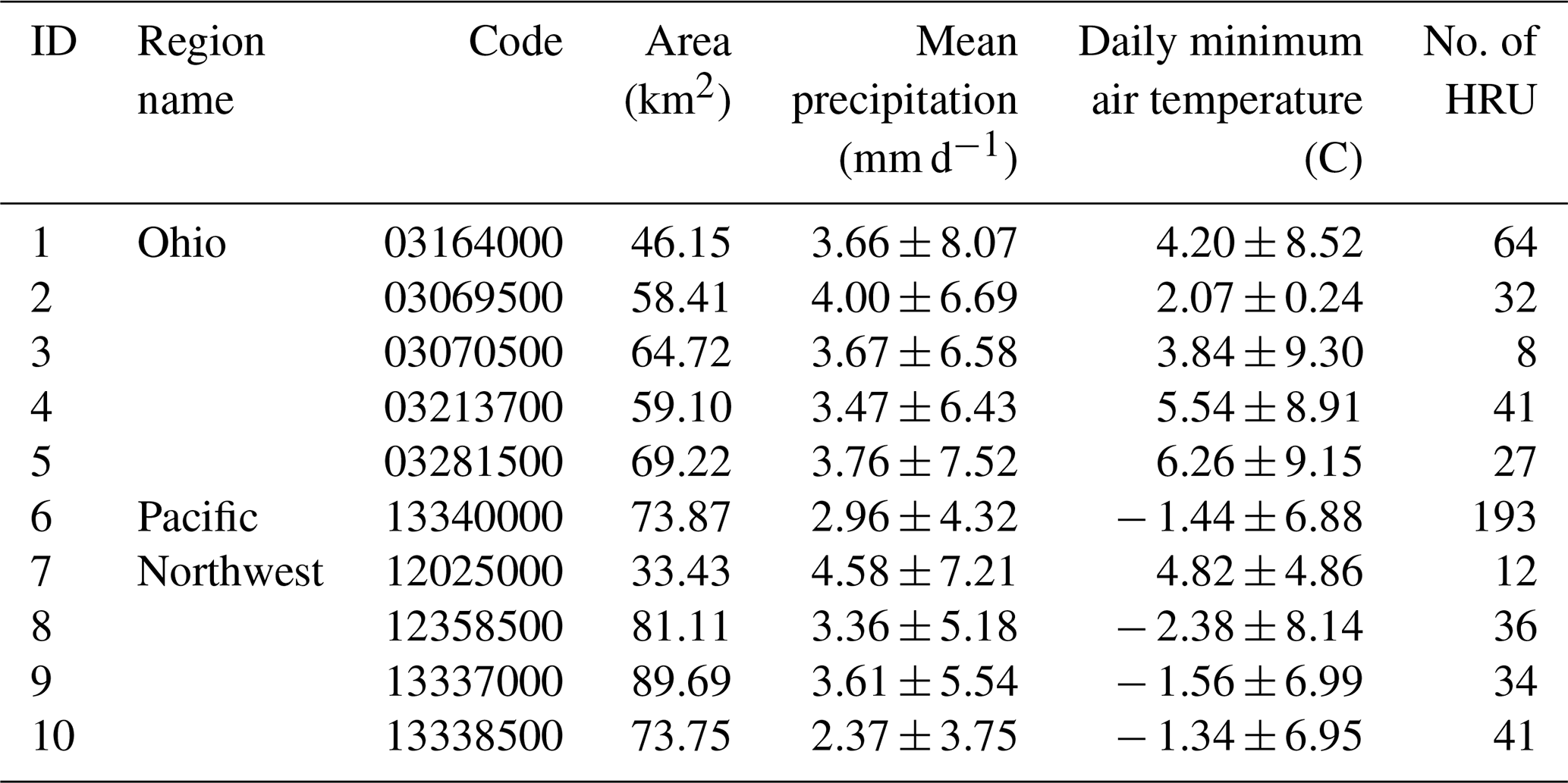
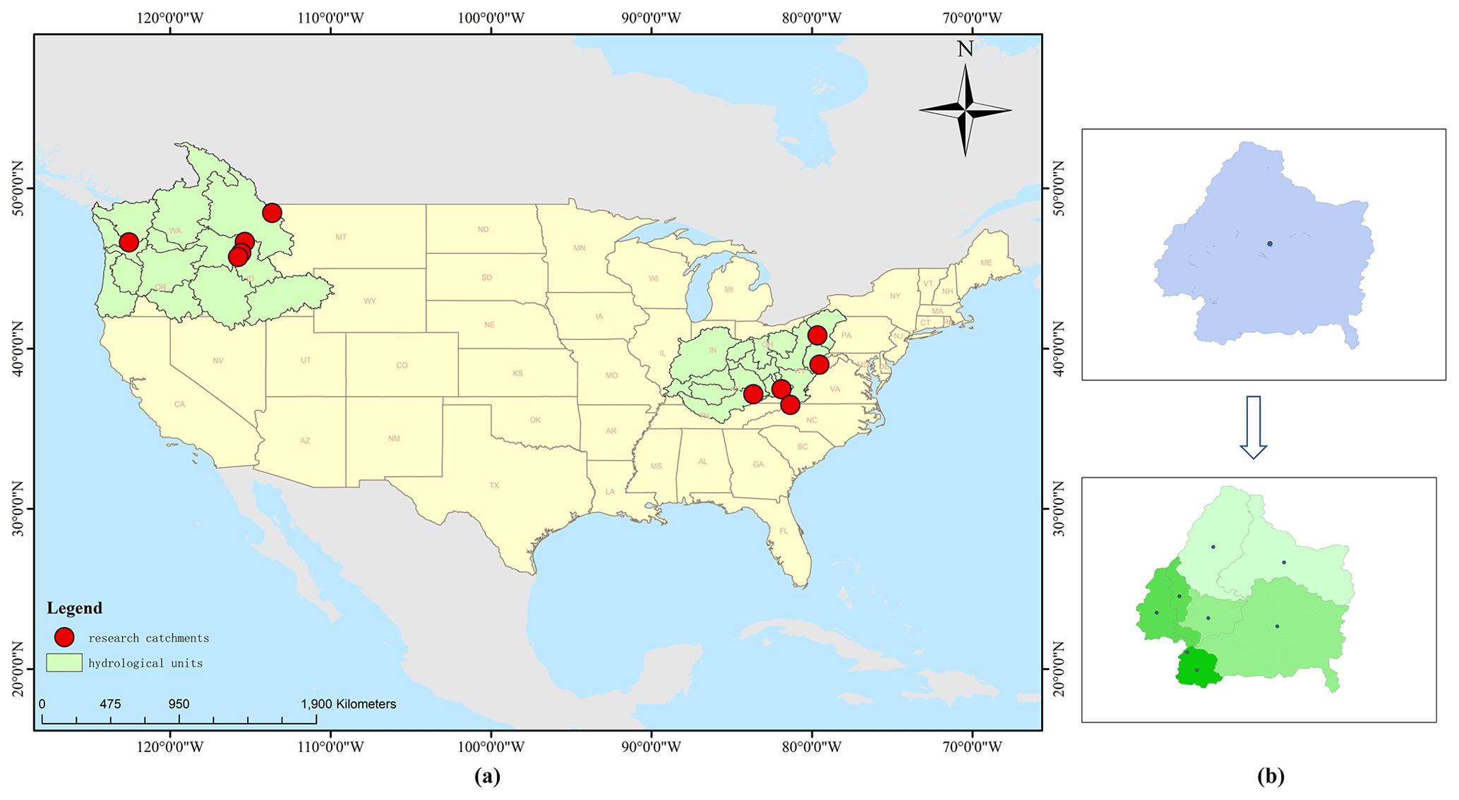
Figure 1 (a) Ten catchments and their locations in the state; (b) examples of spatially distributed rainfall data in this study.

2.2 Long short-term memory network

RNNs are among the most frequently used deep learning models to deal with sequential data. They are a superset of feed-forward neural networks augmented by the inclusion of recurrent edges that span adjacent time steps, introducing a notion of time to the models (Lipton et al., 2015). The main problem with RNN models is the occurrence of long-term dependencies, which arise when the nodes of a neural network have gone through many time steps of computation and the features from a relatively long time ago have been covered by the latest features (Sherstinsky, 2020; Bengio et al., 1994). The main problem with RNN models is the occurrence of long-term dependencies, which arises when the nodes of a neural network have gone through many time steps of computation and the features from a relatively long time ago have been covered by the latest features. The motivation for an LSTM model is to solve the problem mentioned above. As the name implies, long short-term memory is a neural network with the ability to remember both long- and short-term information. LSTM was first proposed by Hochreiter and Schmidhuber (1997) in 1997 and has since gone through several generations, resulting in a more systematic and complete LSTM framework that has been widely used in many fields. The reason why LSTM can solve the long-term dependency problem of RNN is that LSTM introduces the gate mechanism for controlling the delivery and loss of features. The basic structure of LSTM is shown in Fig. 2. In the equations below, Ws are the weight matrices for different gates (W_f for forget gate, W_i for input gate, W_c for output gate, and W_o for gate unit); bs are the bias vectors for different gates (b_f for forget gate, b_i for input gate, b_c for output gate, and b_o for gate unit); tanh is the hyperbolic tangent activation function; and σ is the sigmoid activation function.

Figure 2 Basic LSTM layer structure with a detailed calculation illustration shown in the LSTM cell at time step t.

Whenever information passes through an LSTM cell, there are actions that determine what old information is discarded and what new information is added. The structures that control the addition and subtraction of information to and from the cell state are called gates. There are three such gates in an LSTM cell, namely forget gate, input gate, and output gate.

The forget gate determines which information needs to be noted and which can be ignored. The information from the current input x_t and the hidden state h_t−1 is passed through the sigmoid function. Sigmoid generates a value between 0 and 1, which can be used to describe whether a part of the old output is necessary (by bringing the output closer to 1). This value of f_t is the output of the forget gate.

$$\begin{array}{}\text{(1)}& {\mathit{f}}_t=\mathit{\sigma }\cdot \left({\mathbf{W}}_{\mathrm{f}}\cdot \left[h_{t-\mathrm{1}},x_t\right]+{\mathit{b}}_{\mathrm{f}}\right)\end{array}$$

The input gate performs two steps to update the cell state. First, the current state x_t and the previously hidden state h_t−1 are passed to a second sigmoid function. Next, the same information about the hidden state and the current state is passed through the tanh function. To regulate the network, the tanh operator creates a vector c_t, where all possible values are between −1 and 1.

$$\begin{array}{}\text{(2)}& {\displaystyle }{\mathit{i}}_t=\mathit{\sigma }\cdot \left({\mathbf{W}}_{\mathrm{i}}\cdot \left[h_{t-\mathrm{1}},x_t\right]+{\mathit{b}}_{\mathrm{i}}\right)\text{(3)}& {\displaystyle }\stackrel{\mathrm{‾}}{{\mathit{c}}_t}=\tanh \cdot \left({\mathbf{W}}_{\mathrm{c}}\cdot \left[h_{t-\mathrm{1}},x_t\right]+{\mathit{b}}_{\mathrm{c}}\right)\end{array}$$

The next step is to decide on and store the information from the new state in the cell state c_t. The previous cell state c_t−1 is multiplied by the forget vector f_t. If the result is 0, the information is removed from the cell state. Next, the network takes the output value of the input vector i_t, which updates the cell state and thus provides the network with a new cell state c_t.

$$\begin{array}{}\text{(4)}& {\mathit{c}}_t={\mathit{c}}_{t-\mathrm{1}}\odot {\mathit{f}}_t+\stackrel{\mathrm{‾}}{{\mathit{c}}_t}\odot {\mathit{i}}_t\end{array}$$

The output gate will determine the value of the next hidden state, which contains information about the previous input. First, the model passes the current state and the value of the previous hidden state to a third sigmoid function. The resulting new cell state is then passed through the tanh function. Based on this output value, the network decides what information the hidden state should have. This hidden state is used for output. The new cell state and the new hidden state are transferred to the next time step.

$$\begin{array}{}\text{(5)}& {\displaystyle }{o}_t=\mathit{\sigma }\cdot \left({\mathbf{W}}_{\mathrm{o}}\cdot \left[h_{t-\mathrm{1}},x_t\right]+{\mathit{b}}_{\mathrm{o}}\right)\text{(6)}& {\displaystyle }{h}_t=o_t\odot \tanh \left({\mathit{c}}_t\right)\end{array}$$

In summary, the forget gate determines what relevant information from previous steps is needed. The input gate determines what relevant information can be added to the current step, and the output gate ultimately determines the next hidden state.

2.3 Performance evaluation criteria

In this study, the performance of each model is evaluated by statistical error measurements and characteristics of discharge process error including the Nash–Sutcliffe efficiency coefficient and root mean square error (RMSE).

The Nash–Sutcliffe efficiency coefficient (NSE) is often used to verify the

goodness of the hydrological model simulation results. NSE is calculated as follows:

$$\begin{array}{}\text{(7)}& \mathrm{NSE}=\mathrm{1}-{\displaystyle \frac{{\sum }_{\mathrm{1}}^n(p^t-q^t{)}^{\mathrm{2}}}{{\sum }_{\mathrm{1}}^n(p^t-\stackrel{\mathrm{‾}}{q^t}{)}^{\mathrm{2}}}},\end{array}$$

where p is the model simulation discharge at time t, q^t is the observed discharge at time t, and $\stackrel{\mathrm{‾}}{q^t}$ is the mean of observed discharge. NSE takes the value of negative infinity to 1. NSE close to 1 means that the model quality is good and credible; NSE close to 0 means that the simulation results are close to the mean level of the observed values, i.e., the overall results are credible, but the simulation error is large. If NSE is much less than 0, the model is not credible.

The RMSE assesses how well the predictions match the observations. Depending on the relative range of the data, values can range from 0 (perfect fit) to +∞ (no fit). RMSE is calculated as follows:

$$\begin{array}{}\text{(8)}& \mathrm{RMSE}=\sqrt{{\displaystyle \frac{{\sum }_{\mathrm{1}}^n(p^t-q^t{)}^{\mathrm{2}}}{n}}},\end{array}$$

where p^t is the model's simulation discharge at time t, q^t is the observed discharge at time t, and n is the length of the sequence.

We also used the error of peak discharge (EPD) to measure the ability of the model to simulate peak discharge. Since there are multiple peak discharges in the sequence, we used the mean of all peak discharge EPDs as an indicator. EPD can be calculated as follows:

$$\begin{array}{}\text{(9)}& \mathrm{EPD}={\displaystyle \frac{\mathrm{1}}{n}}\cdot \sum _{\mathrm{1}}^n{\displaystyle \frac{\left|p_{\mathrm{p}}^t-q_{\mathrm{p}}^t\right|}{q_{\mathrm{p}}^t}}\cdot \mathrm{100}\mathit{\%},\end{array}$$

where $q_{\mathrm{p}}^t$ is the observed peak discharge at time $t,p_{\mathrm{p}}^t$ is the modelled peak discharge at time t, and n is the number of peak discharges in the dataset.

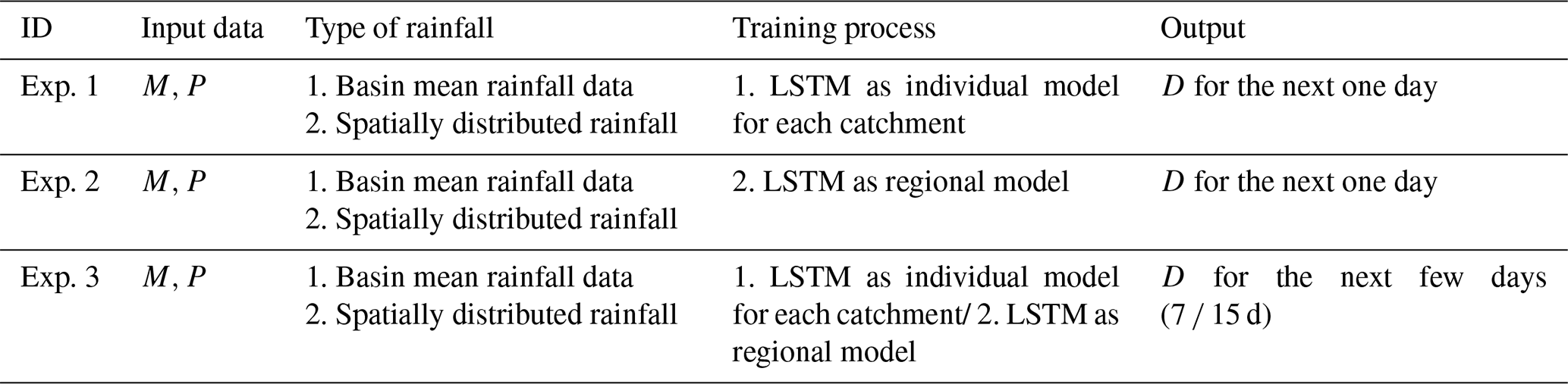
Table 2 Input data, output data, and training process for three experiments.

Figure 3 Comparison of performance of Experiment 1 using different types of rainfall data.

2.4 Experimental setup

Considering the start and end times of rainfall data for all stations in the two catchments, for each catchment, we have a total of 11 680 data points at the daily timescale, which are from 1 January 1980 to 23 December 2011. All model calibration and training was performed using data from 1 January 1980 to 11 October 2008. All model evaluation was done using data from 12 October 2008 to 23 November 2011. All data were normalized before being imported into the model. In this study, we set up three experiments. Experiment 1 and Experiment 2 were used to study the performance of LSTM for “one time step output”. In Experiment 1, LSTM was trained as an individual model in each catchment separately. For each catchment, we used catchment mean rainfall data and spatially distributed rainfall data as input rainfall data. We considered different lengths of the input sequence, mainly 7, 15, 30, 180, and 365 d. In Experiment 2, LSTM was used as a regional model. Specifically, training data from catchments 1–5 were combined to train regional model 1, and training data from catchments 6–10 were combined to train regional model 2. The trained regional model was used for the corresponding catchment in order to test the effect of the model. For each regional model, we used different types of rainfall data separately. It is noted that the vector length used to describe the rainfall spatial distribution information is not consistent for each catchment due to the inconsistent number of HRUs contained in each catchment. When using the regional LSTM, we need to keep the vector lengths of the corresponding catchments the same, so that we can gather the data from different catchments together to train the model. We standardized the length of spatially distributed rainfall data for each catchment to 20 when using the regional LSTM. For the catchment whose length is greater than 20, we fused some of the hydrological response units and take the average value as the rainfall of the fused units. For the catchment whose length is less than 20, we added enough 0 elements to the vector to make the length 20. Experiment 3 was designed to examine the performance of LSTM for “n time step output”. In Experiment 3, the look-back window of the LSTM was set to 365 d based on the results of the first two experiments. We examined the model for the next 7 and 15 d and considered the difference between LSTM as an individual model for each catchment and a regional model. Each model was also driven separately using different rainfall data. We used M for meteorological data including daily minimum air temperature, daily maximum air temperature, mean short-wave radiation, and vapor pressure; D for discharge data, and P for rainfall data. The input and output data for the three experiments (Experiments 1–3) are shown in Table 1. We tested two-layer LSTM with hidden states of 64 and 128, and batch sizes of 64 and 128. Finally, in all experiments, we used a two-layer LSTM structure with a cell/hidden state of 128 for each layer. The dropout rate was set at 0.2 in the experiment, and the batch size was 128. For each training procedure in the three experiments, the number of epochs is 200. We repeated each training procedure 10 times and selected the best-performing model parameters by validation data for the future test.

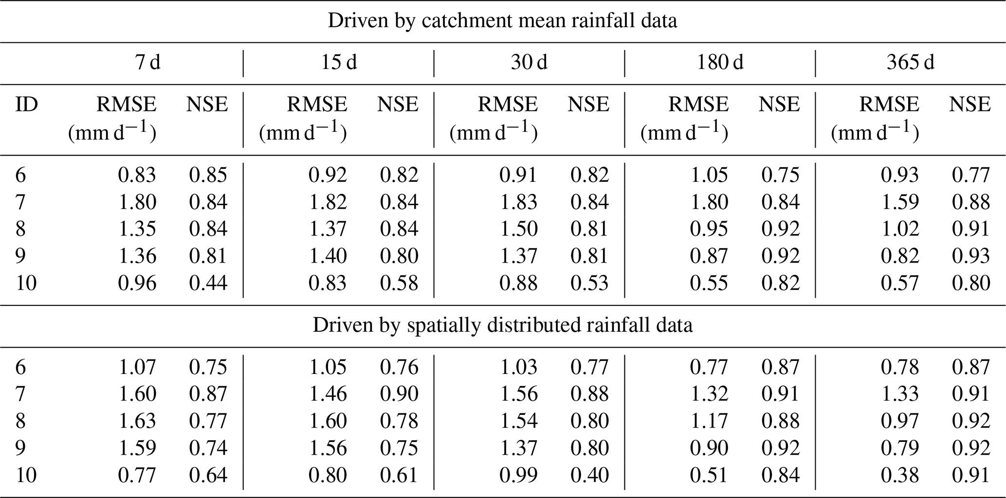
Table 3 Performance of Experiment 1 driven by catchment mean rainfall data.

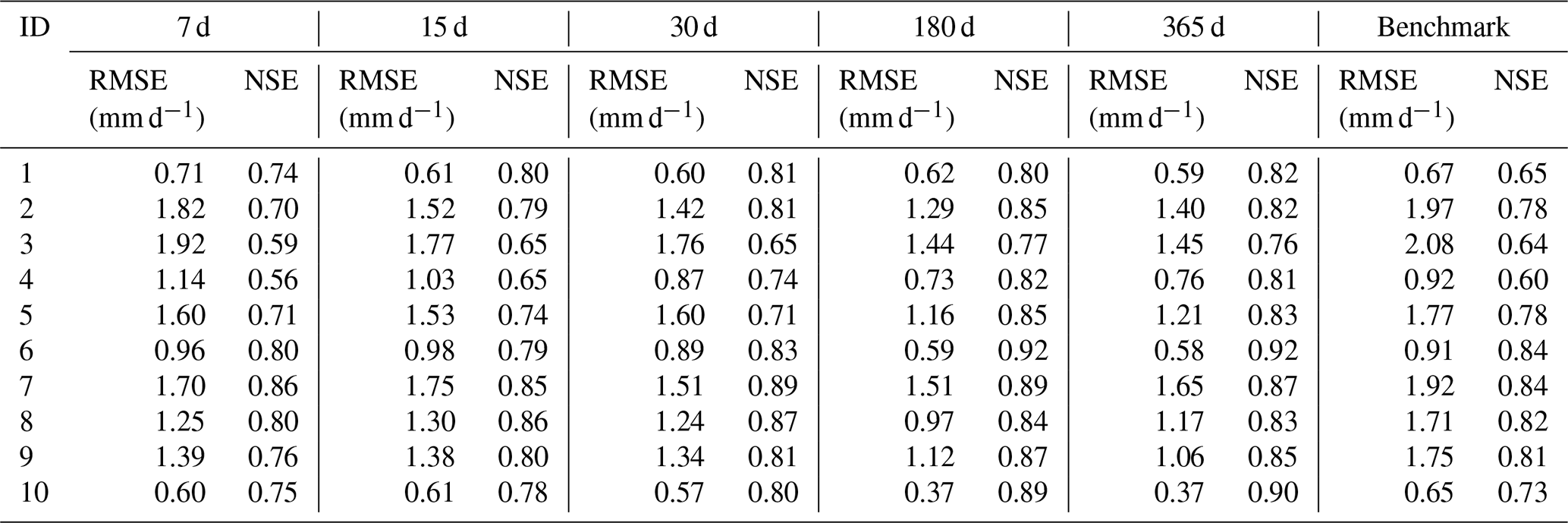
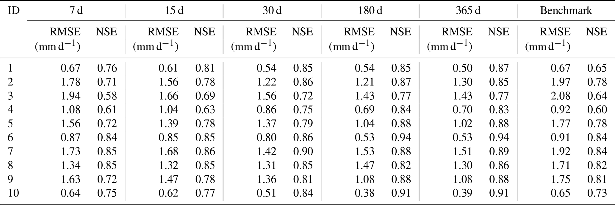
Table 4 Performance of Experiment 1 driven by spatially distributed rainfall data.

3 Results and discussion

3.1 Comparison of the results from different types of rainfall-driven data for “one time step output” simulation using LSTM as individual model (Experiment 1)

In Experiment 1, each catchment was trained separately. We compared the model results for different look-back windows driven by different types of rainfall data. The simulation results of the hydrological model are also placed in each table for comparison. Table 3 shows the performance of Experiment 1 driven by catchment mean rainfall data. From the table, we can see that there is a gradual improvement in the performance of the simulation as the length of look-back windows increases. Except for catchment 7, where the best model occurs at look-back windows of 30 and 180, the best results for all other catchments are at look-back windows of 180 and 365 d. The catchment with the largest improvement in RMSE is catchment 3, where the RMSE is 1.92 with a look-back window of 7 d and 1.45 with a look-back window of 365 d. The catchment with the largest improvement in NSE is catchment 4, where the NSE is 0.56 with a look-back window of 7 d and 0.81 with a look-back window of 365 d. Comparing the results of the LSTM model with the benchmark, we can see that the results of the LSTM model are overall better than those of the benchmark. When the look-back window is 7 or 15 d, the results of some catchments are slightly worse than the benchmark, such as for catchment 4 and catchment 1. However, when the look-back window is larger than 15 d, the results of LSTM outperform the benchmark.

Table 5 Comparison of EPDs of Experiment 1 using different types of rainfall data.

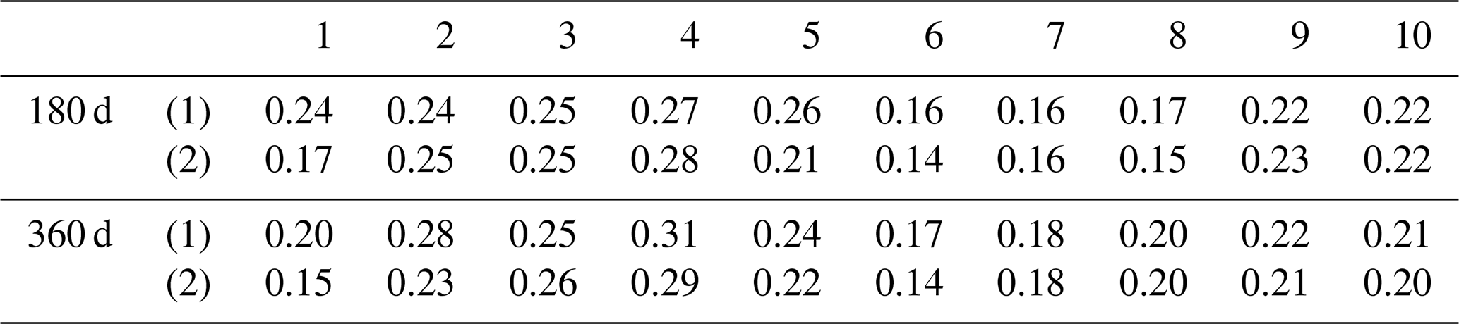
(1) driven by catchment mean rainfall data; (2) driven by spatially distributed rainfall data.

Figure 4 Comparison of performance of Experiment 1 using different types of rainfall data.

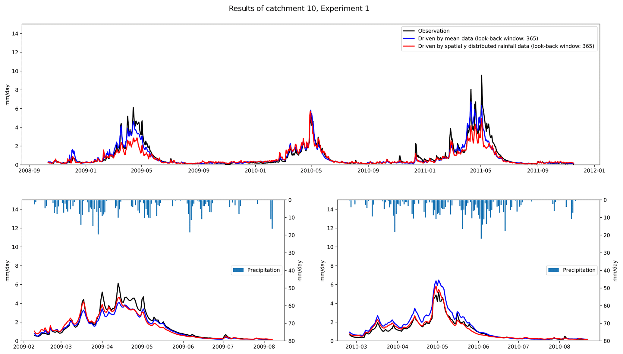
Table 4 shows the performance of Experiment 1 driven by spatially distributed rainfall data. We can see that for the LSTM driven by spatially distributed rainfall data, the results are better than for the shorter look-back windows when the look-back window is 180 or 365 d. For example, for catchment 2, the RMSE for look-back windows of 7 and 365 d are 1.78 and 1.30, respectively, with an improvement of 0.48. The largest improvement in NSE is with catchment 4, with an NSE of 0.56 when the look-back window is 7 and 0.81 when the look-back window is 365. We also compared the results of LSTM with the benchmark. The results are similar to those driven by catchment mean rainfall data. The results of the LSTM model are generally better than the benchmark. Based on the results in Tables 3 and 4, we can conclude that for runoff simulation, increasing the look-back window can improve the simulation performance of the LSTM. In our experiments, regardless of the type of rainfall data used to drive the LSTM, the simulations with look-back windows of 180 and 365 d outperform the models with 7, 15, and 30 d. Compared with RNN, LSTM can learn long-term dependence. The long look-back window can provide more information for establishing the relationship between the input and output data, which can improve the performance of the model.

Figure 5 Comparison of performance of Experiment 1 using different look-back windows.

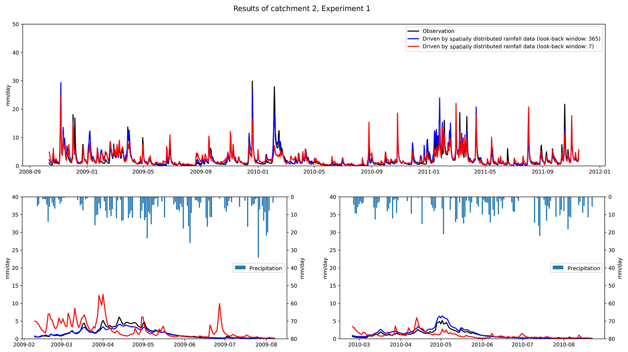
Table 6 Comparison of performance of the regional model (HUC 1) using different types of rainfall data.

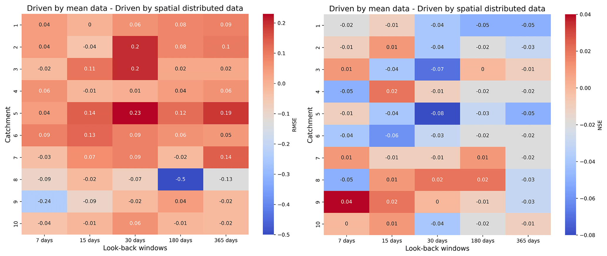
Figure 3 shows how we compare the differences in the results obtained by driving LSTM with different types of rainfall data. The comparison for RMSE is shown in the left panel. Positive values indicate that the results driven by spatially distributed rainfall data are better than those driven by mean rainfall data. The right panel shows the comparison of NSE. Negative values indicate that the results driven by spatially distributed rainfall data outperform mean rainfall data-driven results. We find that the results driven by spatially distributed rainfall data are better than those driven by mean rainfall data. In particular, when the look-back windows are 180 and 365 d, which represent the better models for each catchment, the results driven by spatially distributed rainfall data are generally better than the results driven by mean rainfall data. For example, for NSE, when the look-back window is 365 d, the results obtained from spatially distributed rainfall data are better than those obtained from mean rainfall data. However, we find that for catchment 8, the RMSE obtained for the mean rainfall data with a look-back window of 180 d is 0.5 smaller than the one obtained for the corresponding spatially distributed rainfall data, which is the largest difference.

Table 5 compares the error of peak discharge obtained from different types of driver data. As can be seen from the table, the simulation of peak discharge is better in the results obtained using spatially distributed rainfall data. Except for catchment 4, where the best simulation results occur in the mean rainfall data, the best results for the other nine catchments occur in the results of spatially distributed rainfall data. Figure 4 compares the catchment 10 discharge process using different types of rainfall data. We can see that the discharge process obtained by spatially distributed rainfall is closer to the actual one. The results obtained by spatially distributed rainfall are also better in the simulation of flood peaks. Coupling NSE with RMSE, we can see that good performance can be achieved by using LSTM for runoff simulation. The results of LSTM using longer look-back windows are generally better than those of the benchmark and shorter look-back windows. The spatially distributed rainfall data can provide more information to the input data, which helps the LSTM to better identify the relationship between the input and output data, and thus build a more accurate model.

Table 7 Comparison of performance of the regional model (HUC 2) using different types of rainfall data.

3.2 Comparison of the results from different types of rainfall-driven data for “one time step output” simulation using LSTM as regional model (Experiment 2)

In Experiment 2, we examined the effect of different types of rainfall data on the model when the LSTM is used as a regional model. The data from catchments 1–5 were used together to train regional model HUC 1, and the data from catchments 6–10 were used together to train regional model HUC 2. We applied the trained model to each catchment separately and compared the performance.

Tables 6 and 7 show the results obtained by training the regional model with different types of rainfall data. Firstly, combining the results of the two regional models, we can see the same trend as in Experiment 1, that is, for each model, the optimal performance occurs when the look-back windows are 180 and 365 d. This also proves that extending the look-back windows can improve the model's performance. For HUC 1, we found that spatially distributed rainfall data in all catchments achieved better results, except for catchment 2, where mean rainfall data achieved slightly better simulation results. Similarly, we found that in HUC 2, except for catchment 8, where the mean rainfall data obtained slightly better results than the spatially distributed rainfall data, the spatially distributed rainfall data also obtained better results. Figure 6 shows the EPDs of HUC 1 and HUC 2, where we only count the results for the look-back windows of 180 and 365 d, where the models are more effective. From the figure, we can see that for both HUCs, the EPDs obtained by training the models with spatially distributed rainfall data are generally smaller than those obtained by training with catchment mean rainfall data. This illustrates that adding information on the spatial distribution of rainfall can also improve the simulation of the model when the LSTM is used as the regional model.

Figure 6 Comparison of EPDs of Experiment 2 using different types of rainfall data.

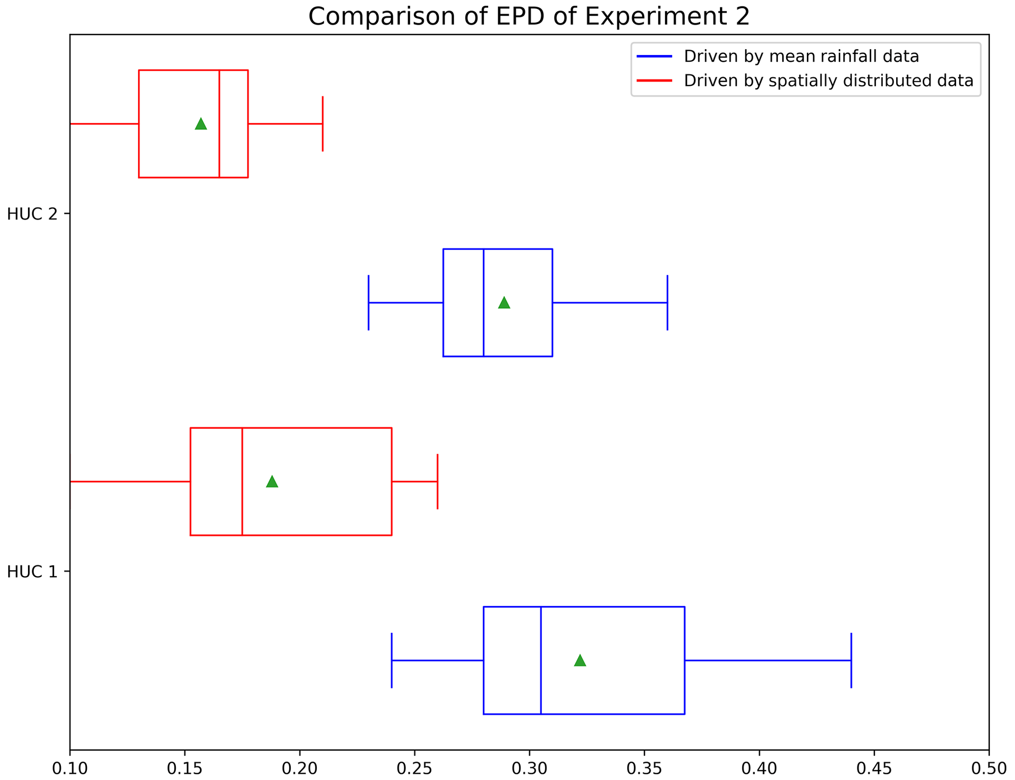
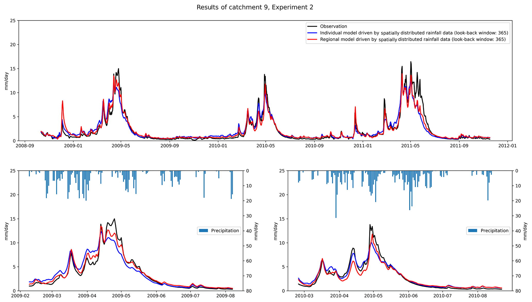
Figure 7 Comparison of performance of Experiment 2 using LSTM as regional model and individual model.

Table 8 Comparison of the performance between using LSTM as a regional model and an individual model: (1) driven by catchment mean rainfall data; (2) driven by spatially distributed rainfall data.

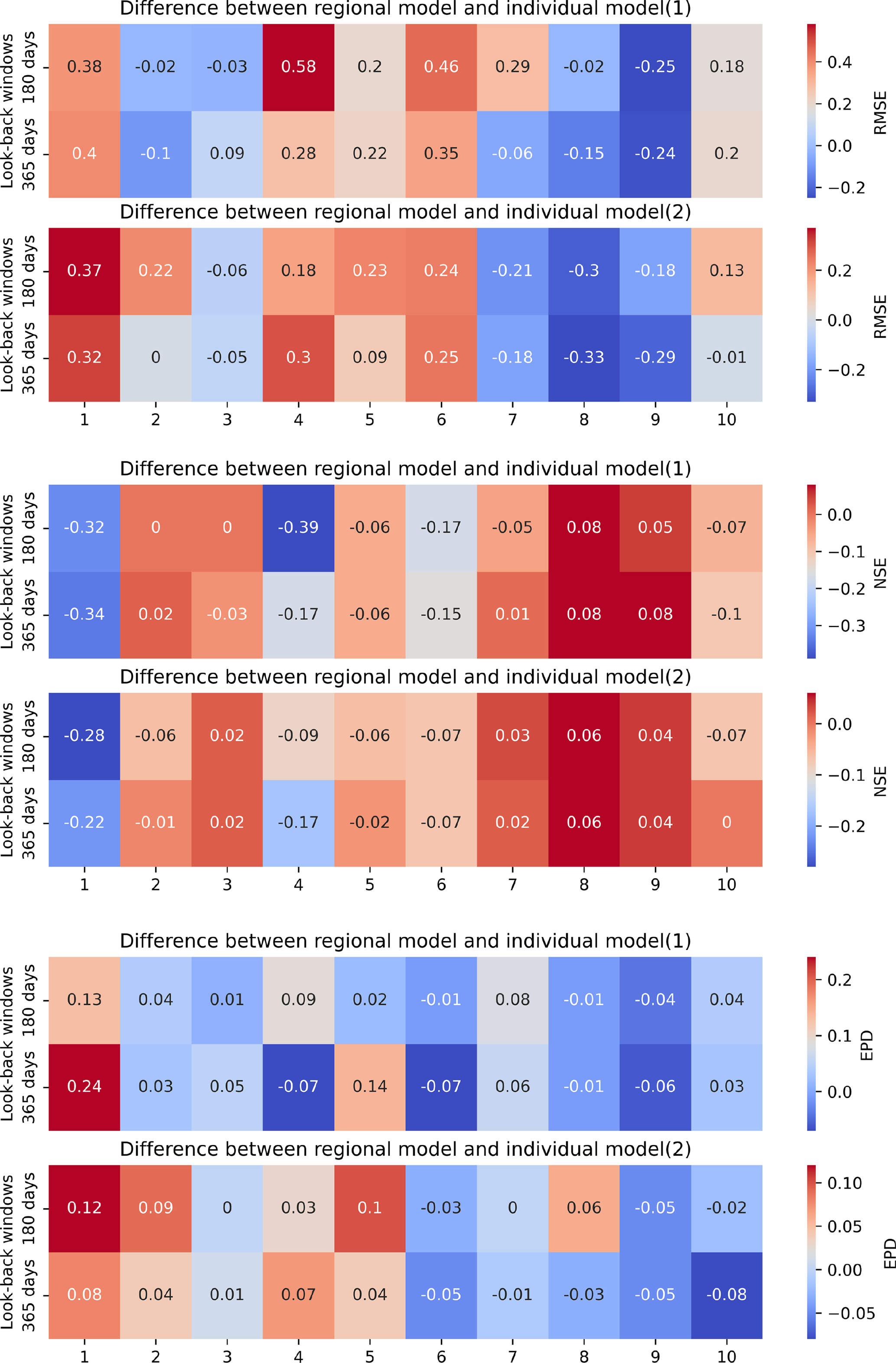
Table 9 Comparison of performance using LSTM as an individual model for “n time step output”.

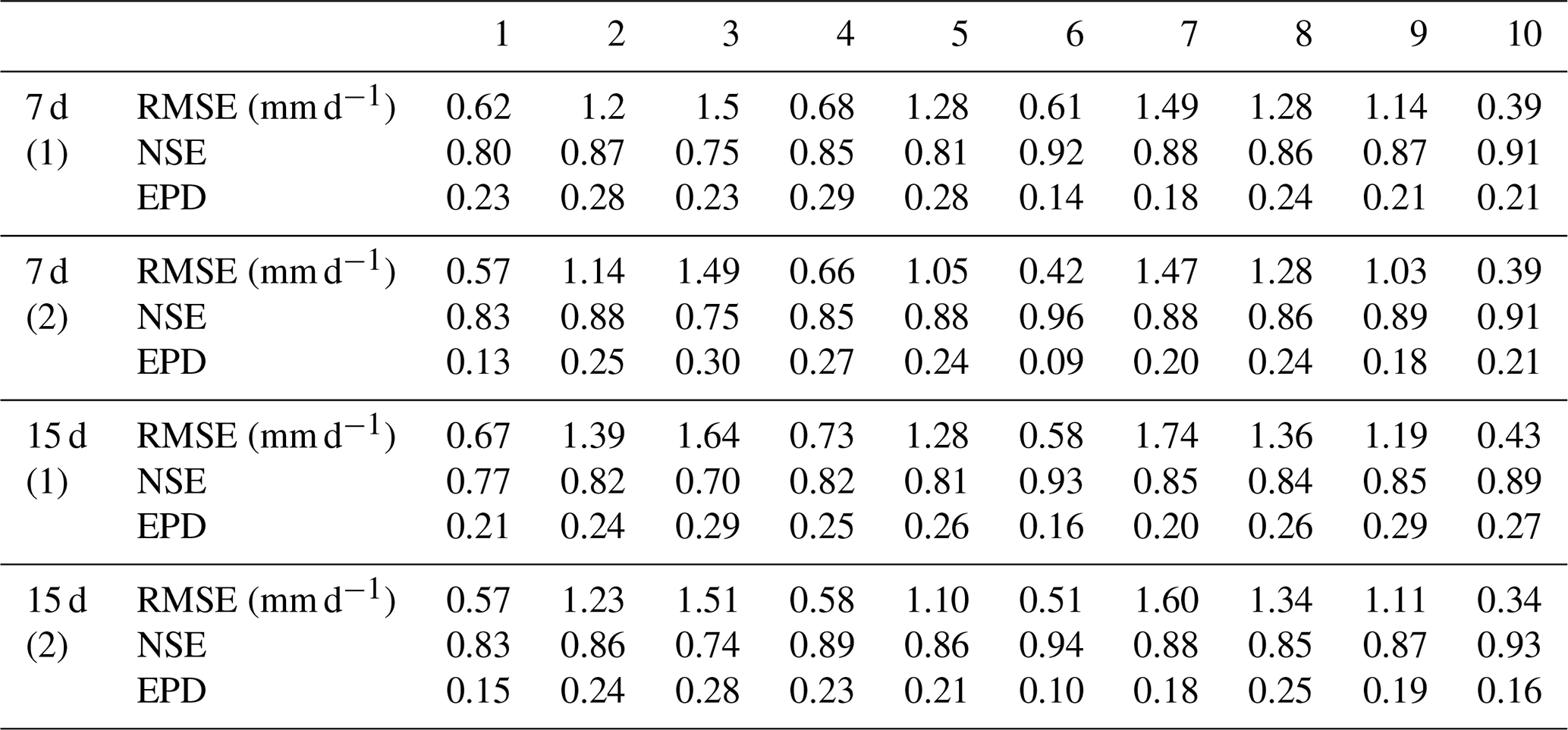
(1) driven by catchment mean rainfall data; (2) driven by spatially distributed rainfall data.

The LSTM as a regional model is a widely used method for runoff simulation. One of the main reasons is that sufficient training data is a prerequisite for a deep learning model to achieve good results, and using data from different catchments of the same hydrological unit can increase the amount of training data. Here, we compare the results obtained by using LSTM as a regional model with those obtained by using LSTM as an individual model for each catchment. Table 8 shows the differences between the three metrics. In the table, a positive value of RMSE means that the regional model is worse than the individual model; a positive value of NSE means that the regional model is better than the individual model; a positive value of EPD means that the regional model is worse than the individual model. From the figure, we did not observe the general phenomenon that LSTM as a region model achieves better results than an individual model. For example, for catchments 1, 4, 5, 6, and 10, the RMSE and NSE using the LSTM as an individual model for each catchment are better than the LSTM as a regional model. This result is consistent for two different types of derived data. One possible reason is that although LSTM as a regional model can be trained with more training data, data from different catchments increase the possibility of inconsistency in the data. Similar discharges may correspond to different input data in different catchments, and similar inputs may correspond to different discharges in different catchments. This may have a negative impact on the learning process of LSTM. However, when comparing the difference of LSTM as a regional model and LSTM as an individual model from different types of data, we find that using spatially distributed rainfall data can reduce the difference between LSTM as a regional model and LSTM as an individual model. We counted the absolute values of different metrics in Table 8. The RMSE, NSE, and EPD between LSTM as a regional model and LSTM as individual model are 0.2 ± 0.15, 0.11 ± 0.11, and 0.06 ± 0.05, respectively, when using mean rainfall data to drive the model. When a spatially distributed rainfall data-driven model is used, the RMSE, NSE, and EPD between LSTM as a regional model and LSTM as an individual model are 0.19 ± 0.10, 0.07 ± 0.07, and 0.04 ± 0.03, respectively.

Table 10 Comparison of performance using LSTM as a regional model for “n time step output”.

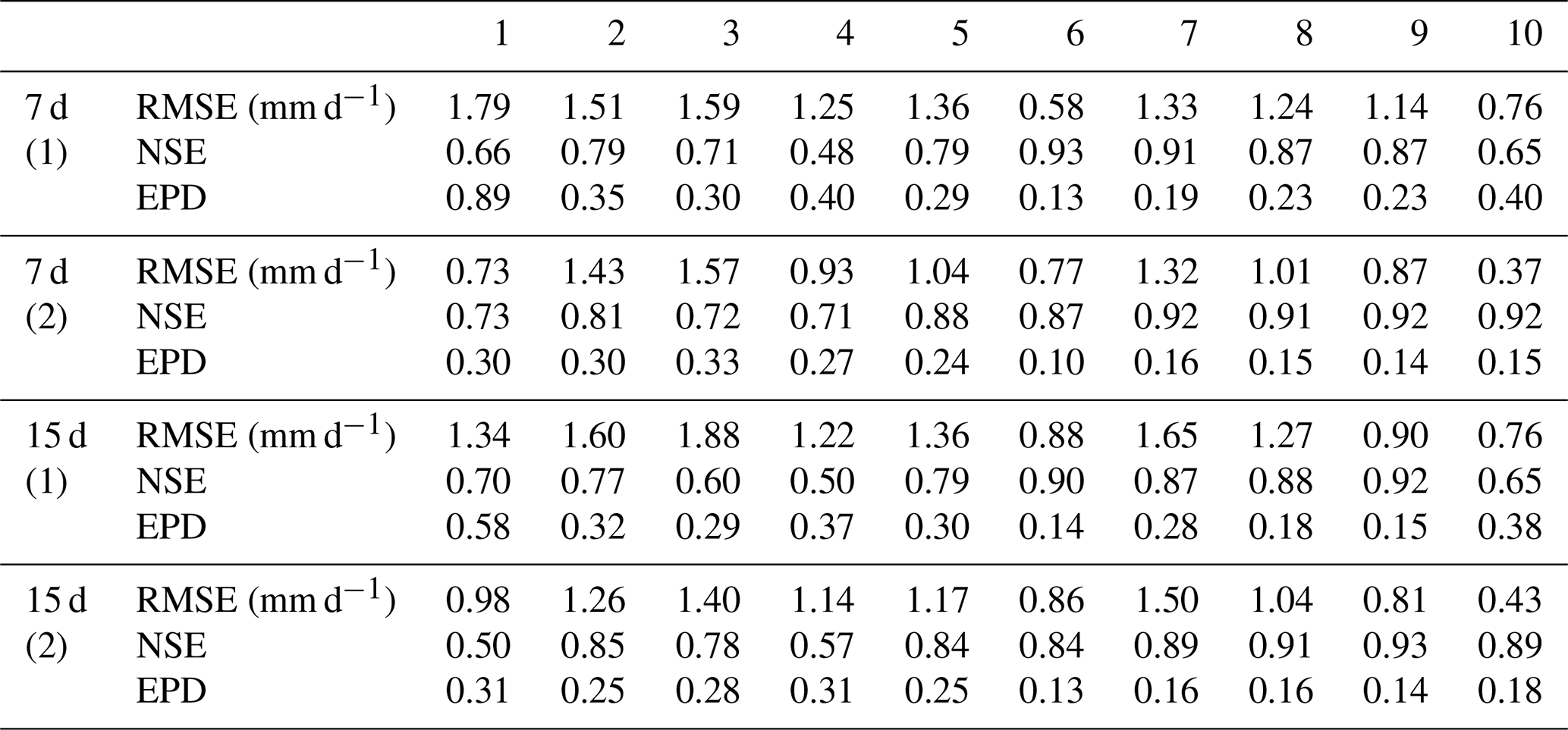
(1) driven by catchment mean rainfall data; (2) driven by spatially distributed rainfall data.

3.3 Comparison of the results from different types of rainfall-driven data for “n time step output” simulation (Experiment 3)

In Experiment 3 we tested the simulation ability of LSTM for n time steps output. Based on the results of Experiment 1 and Experiment 2, we found that longer look-back windows can achieve better simulation results. For the future multi-day simulation, we used a look-back window of 365 d. Our goal is to simulate the future 7 and 15 d discharges. The results of using LSTM as an individual model are shown in Table 9. We can see that the error obtained by simulating the discharge for the next 7 d is smaller than the error obtained by predicting the discharge for the next 15 d. Prediction for multiple days in the future is a much more difficult task. Comparing the simulation results of mean rainfall data and spatially distributed rainfall data, we find that the results obtained by using spatially distributed rainfall data are better than those obtained by using mean rainfall data. For the next 7 d of simulations, catchments 8 and 10 have the same results for different types of driven data. For the next 15 d of simulations, the results obtained for spatially distributed rainfall data in all catchments are significantly better than those obtained for mean rainfall data.

Table 11 Comparison of Experiment 3 between using LSTM as a regional model and an individual model: (1) driven by catchment mean rainfall data; (2) driven by spatially distributed rainfall data.

We also examined the simulation results for future multiple days when LSTM is used as a regional model. From Table 10, we can see that in general, the regional model obtained using spatially distributed rainfall data has better simulation results. Except for catchment 6, the best models for the next 7 d are spatially distributed rainfall data-driven models. The spatially distributed rainfall data-driven model has better results for all catchments for the next 15 d. The results for multi-day simulations are the same as those of Experiment 1 and Experiment 2. We can conclude that the rainfall data with spatial distribution information can improve the rainfall simulation results of LSTM. In particular, for the future multi-day simulations, the addition of rainfall data with spatial analysis information lends a significant advantage over the LSTM driven by mean rainfall data. By comparing different types of regional models, we also find that rainfall data with spatial analysis information can also improve the simulation results of LSTM as a regional model.

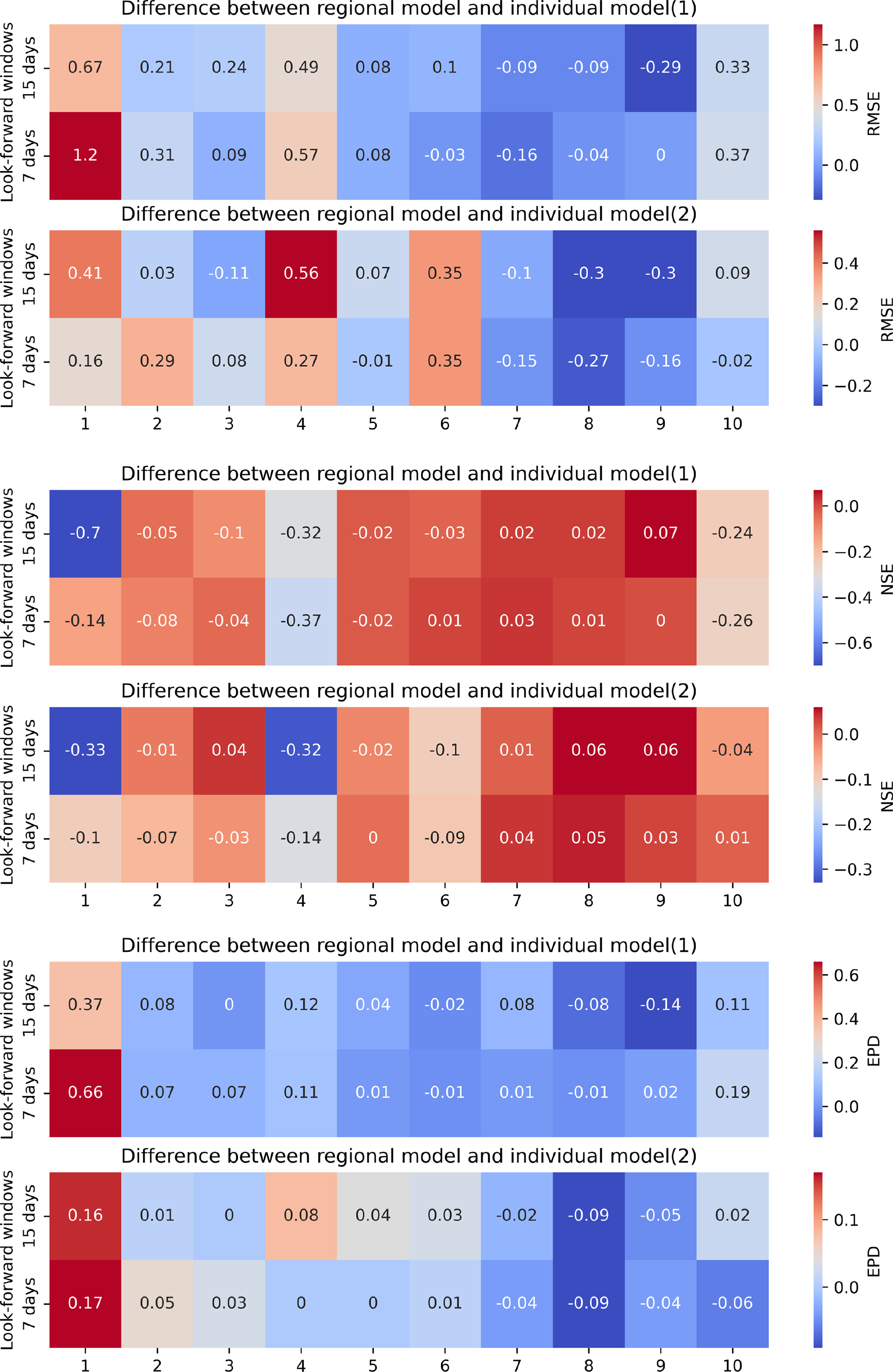
Table 11 shows the comparison of LSTM as an individual model for each catchment and as a regional model for future multi-day simulations. As in Experiment 2, we did not observe a significant advantage of LSTM as a regional model. In general, the regional model is better than the individual model for catchments 7, 8, and 9, which means that the results of the regional model are slightly better than the results of LSTM as an individual model for HUC 2. For catchments 1, 2, 3, 4, and 5, the results of the individual model are generally better than those of the regional model. When comparing the effect of different types of driving data on the differences, we also find that the differences between individual and regional models driven by spatially distributed rainfall data are relatively small.

4 Conclusions and future research

Deep learning models, especially LSTMs, have received increasing attention in rainfall-runoff simulation studies. The current LSTM-based studies are still mainly from a data-driven perspective and few studies have investigated the different simulation results from different types of meteorological data or construction of models based on the physical relationships of rainfall and runoff. In this study, rainfall, which has the greatest influence on runoff, is used as the object of study. The basin mean rainfall data are used as the rainfall data without spatial distribution information, and the vector composed of rainfall on hydrological response units in the catchment is used as the rainfall data with spatial distribution information. The impact of the two types of rainfall data on the performance of the deep learning model is compared and analyzed.

Based on the results of Experiment 1 and Experiment 3, we conclude that the LSTM has a good performance compared to the benchmark when performing runoff simulations. In our experiments, the model performs better with look-back windows of 180 and 365 d than with look-back windows of 7, 15, and 30 d. The trend holds for both 1 d and multi-day simulations. The long look-back window can provide more information for establishing the relationship between the input and output data, which can improve the performance of the model. The trend is not affected by the type of rainfall data.

We used two approaches to train the LSTM model. One is to treat the LSTM as an individual model and train it independently in each catchment. The second is to use the LSTM as a regional model, using data from all catchments in the region for training. Based on the results of Experiment 2 and Experiment 3, we found that regardless of the approach, rainfall data with spatial information can improve the model's performance when compared to the model driven by mean rainfall data. In particular, the spatially distributed rainfall data improves the simulation results more when simulating the next multi-day discharges. The spatially distributed rainfall data can provide more information to the input data, which helps the LSTM to better identify the relationship between input and output and thus build a more robust model. Our findings suggest that increasing the spatial distribution information of the input data can improve the performance of the model, whether the LSTM is used as an individual model or as a regional model for runoff simulation.

We also compared the difference between LSTM as an individual model and LSTM as a regional model. According to the results of our experiments, we did not observe that LSTM as a regional model achieved better results than LSTM as an individual model. In some catchments the regional model gives better results, while in others the individual model gives better results. This conclusion applies to both 1 d and multi-day simulations. However, we found that using spatially distributed rainfall data can reduce the difference between LSTM as a regional model and LSTM as an individual model. Although LSTM as a regional model can be trained with more training data, data from different catchments increase the possibility of inconsistency in the data. Similar discharges may correspond to different input data in different catchments, and similar inputs may correspond to different discharges in different catchments. This may have a negative impact on the learning process of LSTM.

When we compared the results of spatially distributed rainfall data in Experiment 1, i.e., increasing the spatial distribution information of the input data, with the results of mean rainfall data in Experiment 2, i.e., increasing the size of the training data, we found that the results of the two are comparable. The variables related to runoff generation are characterized by uneven spatial distribution, such as rainfall, temperature, humidity, etc. Understanding and utilizing the spatial distribution information of these variables can help improve the performance of deep learning models in runoff simulations. This is especially true for those regions where data are scarce, since raster rainfall data with spatial distribution information are currently available from many sources. Adding information about the spatial distribution of the data is another way to improve the performance of deep learning models.

There are some gaps that can be continued to be investigated in the future. For example, in this study, the rainfall of the hydrological response unit of the catchment is used to represent the spatial distribution of rainfall information. We can obtain raster-type rainfall data from satellite data, climate models, and other sources, which may be able to better represent the spatial distribution of rainfall. We only consider comparing the basin mean rainfall and spatially distributed rainfall; however, other driving data, such as temperature and pressure, also have spatial distribution characteristics. How to increase the spatial distribution information of all features on the basis of the uniform resolution of different features and compare the influence of the input conditions on the model results is also a research direction worth pursuing in the future.