the Creative Commons Attribution 4.0 License.
the Creative Commons Attribution 4.0 License.
 | 27 Apr 2022
Hydrological response of a peri-urban catchment exploiting conventional and unconventional rainfall observations: the case study of Lambro Catchment
Greta Cazzaniga
Carlo De Michele
Michele D'Amico
Cristina Deidda
Antonio Ghezzi
Roberto Nebuloni
Commercial microwave links (CMLs) can be used as opportunistic and unconventional rainfall sensors by converting the received signal level into path-averaged rainfall intensity. As the reliable reconstruction of the spatial distribution of rainfall is still a challenging issue in meteorology and hydrology, there is a widespread interest in integrating the precipitation estimates gathered by the ubiquitous CMLs with the conventional rainfall sensors, i.e. rain gauges (RGs) and weather radars. Here, we investigate the potential of a dense CML network for the estimation of river discharges via a semi-distributed hydrological model. The analysis is conducted in a peri-urban catchment, Lambro, located in northern Italy and covered by 50 links. A two-level comparison is made between CML- and RG-based outcomes, relying on 12 storm/flood events. First, rainfall data are spatially interpolated and assessed in a set of significant points of the catchment area. Rainfall depth values obtained from CMLs are definitively comparable with direct RG measurements, except for the spells of persistent light rain, probably due to the limited sensitivity of CMLs caused by the coarse quantization step of raw power data. Moreover, it is shown that, when changing the type of rainfall input, a new calibration of model parameters is required. In fact, after the recalibration of model parameters, CML-driven model performance is comparable with RG-driven performance, confirming that the exploitation of a CML network may be a great support to hydrological modelling in areas lacking a well-designed and dense traditional monitoring system.
- Article
(3819 KB) - Full-text XML
- BibTeX
- EndNote


Precipitation is the main downward forcing of the water cycle (Kidd and Huffman, 2011) and, consequently, one of the most relevant inputs in hydrological models, which are key tools in early-warning systems for flood risk forecasting and mitigation (EU Water Directors, 2003). However, precipitation exhibits a significant temporal and spatial variation over a catchment area or region (Dawdy and Bergmann, 1969; Bengtsson, 2011; Parkes et al., 2013), and this is a critical aspect leading to difficulties in reconstructing a reliable rainfall field. In the past, several studies have investigated the effects of spatio-temporal variability in rainfall on the hydrological model outputs (e.g. Obled et al., 1994; Bárdossy and Das, 2008; Younger et al., 2009; Arnaud et al., 2011), proving that precipitation inputs have a marked influence on the simulated outflow hydrographs. It is also known that the reconstruction of rainfall input is more accurate as the number of rainfall measurements increases over a study area (Chen et al., 2010; Xu et al., 2013). However, because of economic or geographical factors, an adequate density of rainfall sensors is often not available.
Currently, the most common ground-based technology for rainfall measurement is the rain gauge (RG), which provides single-point measurements (New et al., 2001). In addition, high-precision ground sensors, namely disdrometers, provide the size and velocity of hydrometeors (Jaffrain et al., 2011; Cugerone and De Michele, 2015). One of the major problems encountered when dealing with single-point measurements is the transfer of information to ungauged sites or the reconstruction of the rainfall field over the catchment of interest. Such estimates can be performed by the use of spatial interpolation techniques. Several methods are now available, with different degrees of complexity. They can be either deterministic, such as the inverse distance weighting (IDW) method (Shepard, 1968) and the Thiessen polygon method (Thiessen, 1911), or stochastic, such as the Kriging technique (Delhomme, 1978) and co-Kriging (Myers, 1984). However, the outcome of these techniques has been proven to be highly sensitive to the gauge density (Xie et al., 1996), depending on the temporal resolution. Specifically, the shorter the aggregation time, the more critical the rain gauge density. Alternatively, the rainfall field at ground level can be indirectly obtained by weather radars, when available. The radar retrieves the average rainfall intensity across a volume from measurements of reflectivity through power-law formulas, such as the one proposed by Marshall and Palmer (1948). A recent survey of reflectivity-rainfall intensity formulas is given in Raghavan (2013). Ignaccolo and De Michele (2020) and Jameson and Kostinski (2002) have argued about the purely statistical nature of the reflectivity-rainfall intensity formulas, with important consequences regarding their use where calibration with local data is missing. There are also other drawbacks associated with the use of radar reflectivity, including the problem of spurious echoes, such as ground clutter (Alberoni et al., 2001; Rauber and Nesbitt, 2018), which restrict the use of radars to plain areas, and the fact that the radar reflectivity provides only information about precipitable water. Recently, the dual-polarization upgrade of radars (Zhang et al., 2019; Chen et al., 2021) has added information about the shape, composition, and phase of the hydrometeors. Hence, quantitative precipitation estimation (QPE) has greatly benefited from such advancements.
For all of these reasons, measuring the spatial distribution of rainfall is still an open issue, which may be tackled through the integration of conventional sensors and/or the implementation of new instruments to complement existing measurements. In this context, the use of opportunistic rainfall sensors, such as commercial microwave links (CMLs), has raised considerable interest. CMLs are the point-to-point radio links connecting the base stations of a mobile network to the core infrastructure. The use of microwave links as opportunistic rainfall detectors was firstly proposed by Atlas and Ulbrich (1977). The method exploits the relationship between the rainfall intensity and the attenuation (i.e. the loss of signal power) experienced by the electromagnetic wave along the propagation path from the transmitter to the receiver. Later, Giuli et al. (1991) made use of a mesh of microwave links for the 2D reconstruction of the rainfall field, through simulation. A pioneering experimental campaign was carried out during the Mantissa project (Rahimi et al., 2003). However, at that time, the need to install ad hoc microwave links made the technique impractical. A few years later, the scenario changed following the dramatic expansion of cellular telephony. The use of the ubiquitous CMLs connecting the base stations of cellular networks was first proposed by Messer et al. (2006). Their paper triggered many studies that were conducted worldwide to investigate the potential of CMLs for meteorological and hydrological applications. From a hydrological point of view, CML-based rainfall products were first exploited by Fencl et al. (2013) to improve urban drainage modelling in a small-scale (2.33 km2) impervious catchment in Prague, Czech Republic. Later, Brauer et al. (2016) investigated the effects of the use of CML data in discharge simulations, for a natural lowland catchment in the Netherlands, at a small scale (6.5 km2). A further study by Smiatek et al. (2017) used microwave-link-derived precipitation estimates as rainfall input in a distributed hydrological model applied to the Ammer Basin (Germany), with an area of 609 km2. In that work, the authors employed the IDW method for the interpolation of RG and CML rainfall data on a 100 m×100 m grid. Another case study to check the potential of a dense CML network for urban drainage management was carried out on an agglomeration of cities (16 km2) in the Czech Republic by Stransky et al. (2018). Pastorek et al. (2019) assessed the impact of CML quantitative precipitation estimates (QPEs) on urban drainage modelling. The authors found that the sensitivity of CMLs is the factor that mostly affects the QPEs and that the bias on QPEs propagates throughout rainfall–runoff simulations. Moreover, they showed that the position of CMLs over the drainage area impacts the reconstruction of the runoff dynamic. In Italy, Roversi et al. (2020) conducted a validation of the CML rainfall estimates in the Po Valley (northern Italy) by comparing them with different data sources (RGs, the ERG5 meteorological data set, and radar products). However, to our knowledge, a hydrological application of CML-based rainfall estimates does not currently exist.
Herein, the analysis aims at investigating and validating the potential of a CML network, located in Lombardy (northern Italy), exploited for hydrological purposes. Specifically, relying on a semi-distributed hydrological model, we assessed whether rainfall data collected by a large CML network of 50 links may be used to provide a reliable reconstruction of the hydrological process in a medium-sized basin and if the reconstruction is comparable with those achieved with a well-designed RG network. We investigated a set of summer and autumn precipitation events, both convective and stratiform, that occurred over the Lambro Catchment during the years 2019 and 2020. The analysis of events taking place in different seasons allowed us to point out some limitations of CMLs with respect to detecting specific types of precipitation. In this work we firstly focused on the spatial interpolation of rainfall observations, comparing results from conventional (RGs) and unconventional (CMLs) instruments and their combined use. In fact, the issue of spatial interpolation is crucial when dealing with point (RG) or linear (CML) measurements used as input for a semi-distributed hydrological model, especially when the study area is quite large (in the order of 100 km2 or even larger). We relied on the traditional IDW method to spatially interpolate precipitation measurements/estimates from RGs/CMLs. Secondly, we implemented a semi-distributed rainfall–runoff model using three types of input: (1) RG measurements, (2) CML estimates, and (3) a combination of RG and CML data. Given the different nature of rainfall input, we also assessed three calibrations of model parameters. We then compared results in terms of river discharge.
The remainder of this paper is structured as follows. In Sect. 2, we present the case study, the experimental set-up, and the features of the networks of conventional and unconventional sensors. Section 3 includes a description of all methods implemented for the analysis, and Sect. 4 reports the results, including a comparison of rainfall spatial interpolation carried out with the different data types and of streamflow simulations against hydrometric measurements. Discussion and conclusions are given in Sects. 5 and 6 respectively.
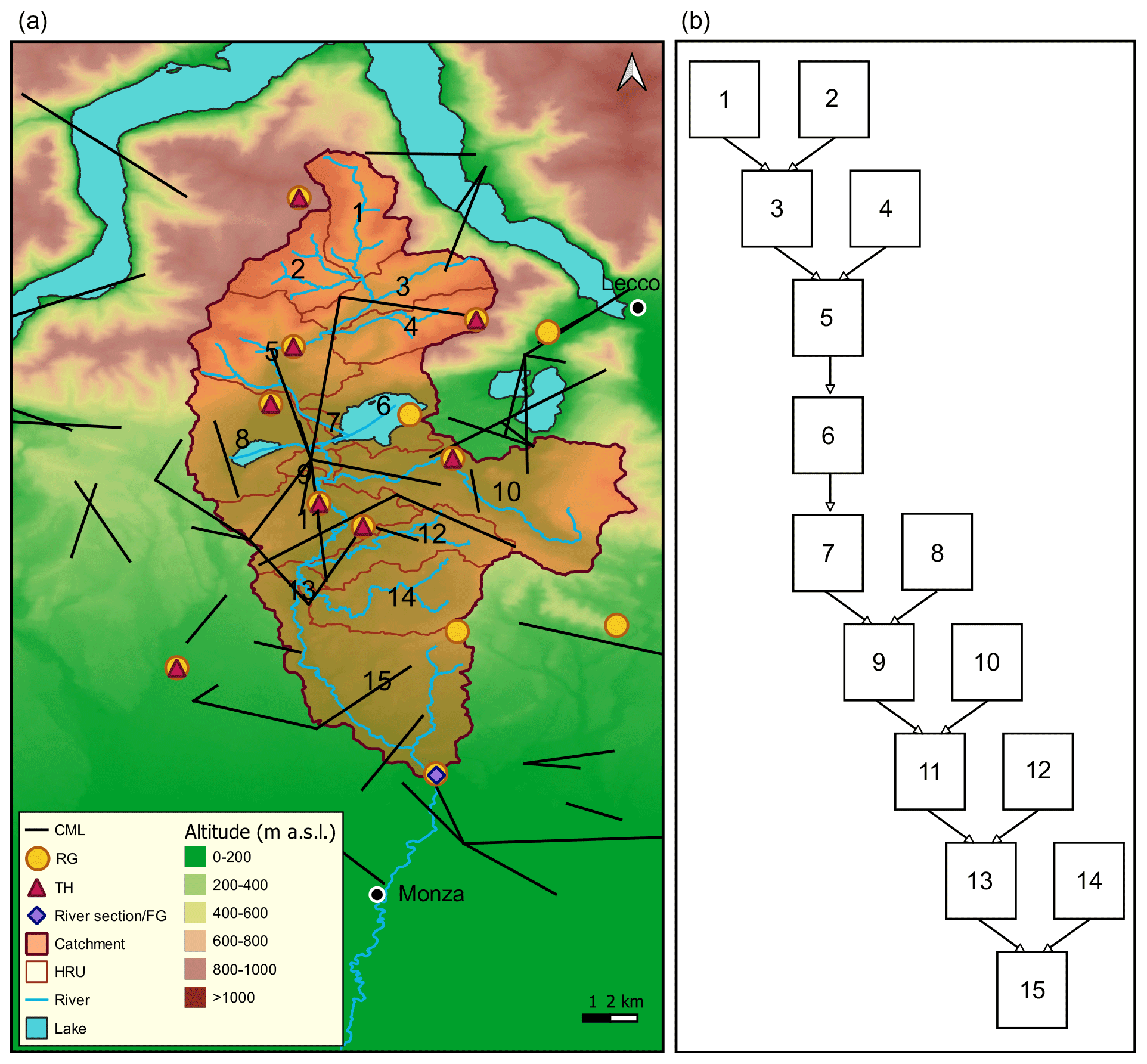
Figure 1Case study area: panel (a) shows the Lambro Catchment, the partitioning into 15 sub-basins (HRUs), and the position of the sensors; panel (b) reports the scheme of HRU interaction in the network. Please note that FG is the flow gauge located at the outlet section. The digital terrain model (DTM) is freely available at https://www.geoportale.regione.lombardia.it (last access: 10 March 2022).
The case study was carried out in the Lambro Catchment, a peri-urban catchment that is a northern tributary of the Po River, as shown in Fig. 1a. It is located north of the Milan metropolitan area and covers three different provinces: Como, Lecco, and Monza and Brianza. The Lambro River, at the Lesmo River section (shown in purple in Fig. 1a), drains an area of 260 km2 that can be mainly divided in two zones based on different morphology and land use. The northern zone is the pre-Alpine region, where the Lambro River originates, at 944 In contrast, the southern zone, between Pusiano Lake (in sub-basin 6 in Fig. 1) and the outlet section, at 178 , is a flat area subjected to massive urbanization, which results in large impervious surfaces and, consequently, fast runoff processes with a lag time of few hours. The catchment includes the presence of two lakes: Pusiano Lake (which is the biggest one) and Alserio Lake (in sub-basin 8 in Fig. 1), both located in the middle part of the catchment. According to the Köppen (1925) climate classification, the northern inland portion of Italy belongs to the humid subtropical climate (Cfa) zone. Heavy convective precipitation cells characterize the basin, while the highest monthly rainfall accumulation occurs in spring and autumn. The local meteorological drivers, along with urban sprawl, lead to the hydrological vulnerability of the region. In order to mitigate hydrological risk in the Monza and Milan urban areas (downstream of our case study region), structural works have been carried out along the Lambro River in past years. Moreover, great efforts have been made in the implementation and development of non-structural measures (e.g. Ravazzani et al., 2016; Masseroni et al., 2017; Lombardi et al., 2018), including a dense monitoring system managed by ARPA Lombardia (the regional agency for environmental protection). From this, we exploited 10 min resolution rainfall depths and temperatures from 13 tipping-bucket RGs and eight thermometers (THs) respectively, for the years 2018 and 2019 as well as for the first 6 months of the year 2020. In addition, we used 10 min resolution water level measurements of a flow gauge (FG), located at the outlet section of the Lambro Basin in the municipality of Lesmo. All of these meteorological and hydrological data are available at https://www.arpalombardia.it (last access: 10 March 2022). A rather dense CML network, owned by Vodafone Italia S.p.A., covers the central and southern catchment area and its surroundings. In contrast, the northernmost portion of the Lambro Basin is covered by few and unevenly distributed CMLs, given that it is thinly populated and characterized by higher altitudes. A total of 50 CMLs are available over the above-mentioned area. The key features of CMLs as rainfall sensors are the operation frequency and the path length. Regrouping the available CMLs according to the frequency:
-
5 links are in the frequency range [11.4,13.1] GHz, with a path length between 3.5 and 8 km;
-
37 links are in the frequency range [18.8,23.0] GHz, with a path length between 1 and 8.5 km;
-
8 links are in the frequency range [38.5,42.6] GHz, with a path length between 1.4 and 2.2 km.
We investigated 12 storm events and the associated floods, in the period from June 2019 to June 2020. The RG- and CML-based precipitation data sets, aggregated at an hourly timescale, cover a wide range of rainy events, from summer thunderstorms to low-intensity autumn events. In Table 1, we reported some features characterizing the 12 selected events, namely the initial date, the final date, and time; the accumulated precipitation averaged over 13 RG measurements; the total volume of precipitation that fell on the basin area; the 1 h maximum rain rate; the observed total flow volume; and the peak flow. We defined a storm event as the time lapse where at least one RG, available in the area, detected precipitation with possible dry intervals no longer than 5 h. An hour is considered dry when the detected rainfall depth is lower than 1 mm and wet otherwise. The beginning of the flood event is conventionally set at the hour in which the flow rate experienced a sudden deviation from the average. The end is instead set when the flow rate reverts to the initial condition, at the end of the depletion curve. According to the maximum observed rain rates, we classified events as low-rain-rate and high-rain-rate events, adapting the classification reported in Met Office (2007) to our specific case study. The former group includes storm events 5, 6, 7, and 12, for which the maximum rain rate was lower than 15 mm h−1, whereas the latter covers the remaining events, for which the maximum rain rate was higher than 15 mm h−1.
In order to implement the hydrological model (see Sect. 3.2), the catchment area is divided into 15 sub-basins (as shown in Fig. 1a), with areas ranging from 1.15 km2 (HRU 7) to 42.6 km2 (HRU 10). Hereinafter, the sub-basins will be referred to as hydrological response units (HRUs). In particular, the semi-distributed model adopted here requires, as input data, rainfall depths estimated in the HRU centroids. The estimates were gathered using the IDW technique (see Sect. 3.3), and a different number of sensors was exploited for each HRU, according to a defined maximum distance of 10 km from the HRU centroid. Figure 2 shows some features of the rainfall sensors used for spatial interpolation in each HRU: the number of exploited RGs, CMLs, and their sum; the ratio between the number of CMLs and RGs; the mean distance between rainfall sensors and HRU centroids; and the mean length of CMLs. Please, note that the CML–HRU centroid distance is calculated considering the CML middle point. It is also worth mentioning that the number of available CMLs was less than 50 for some events due to instrument maintenance or malfunction. Hence, the numbers in Fig. 2 are averaged over all of the events. Figure 2a highlights a significant increase in the exploited CMLs from HRU 1 to 6. This could be a potential problem and could lead to more inaccurate estimates, at the stage of spatial interpolation, for the northern HRUs with respect to the southern ones. On the other hand, the number of RGs undergoes minor variation from one HRU to another. In Fig. 2b, we can see that the lowest ratios between CMLs and RGs correspond to HRU 1 to 5 and HRU 10. Moreover, Fig. 2c shows that, considering HRUs 1 to 9, the mean distance between sensors and HRU centroids is always higher when CMLs are considered. The opposite trend, with a single exception for HRU 12, occurs for HRUs located further downstream. Lastly, the mean CML length, in Fig. 2d, has a decreasing trend from upstream to downstream.
Table 1Details of the 12 events considered. The date, time, cumulative precipitation, precipitation volume, and 1 h maximum rain rate for the 12 storm events are shown on the left, and the date, time, flow volume, and peak flow of the corresponding flood events are shown on the right. Here, LT stands for local time.
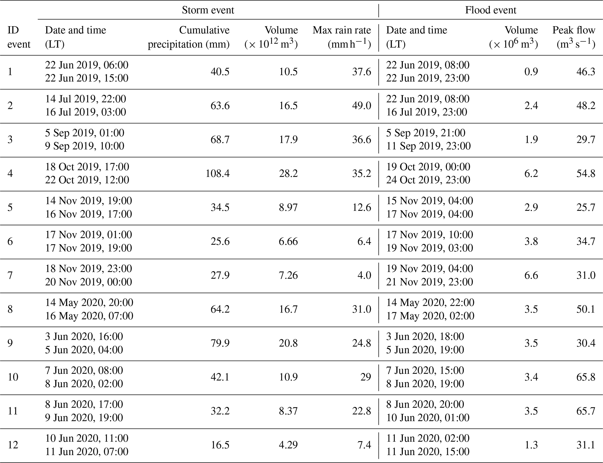
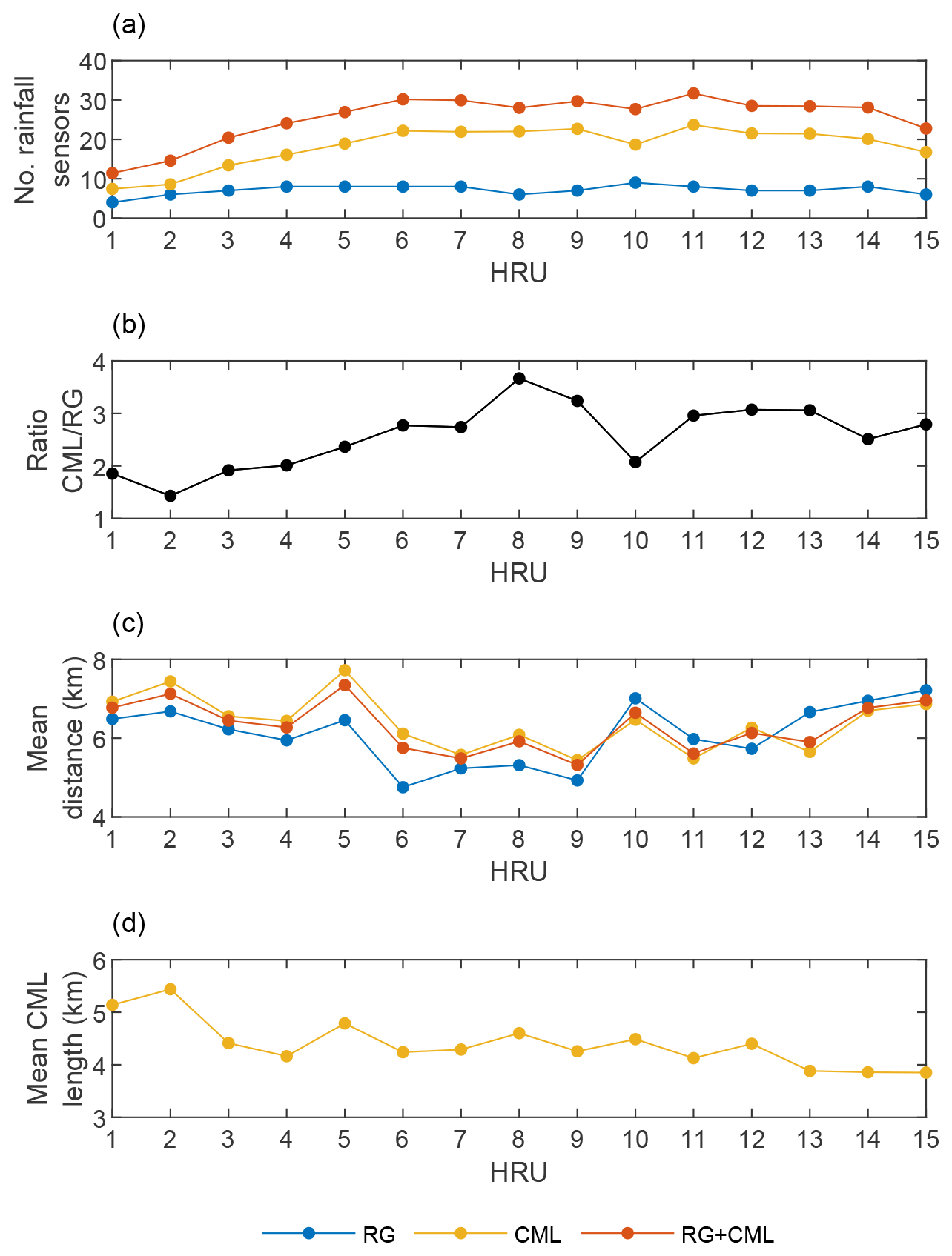
Figure 2Panels (a) to (d) show the number of rainfall sensors used for spatial interpolation in each HRU centroid, the ratio between the number of RGs and CMLs, the mean distance between rainfall sensors and HRU centroids, and the CML mean lengths respectively.
In this section we firstly describe the data processing algorithms. While the procedure is simple for conventional sensors (RGs, THs, and the FG), it is not straightforward to extract quantitative rainfall information from CML raw data, which are generated for network monitoring purposes. Second, we discuss the semi-distributed hydrological model and its calibration/validation procedures. Finally, we illustrate the methods for the spatial interpolation of RG- and CML-based rainfall data.
3.1 Data processing
Conventional sensors (rain gauges, thermometers, and the flow gauge)
Raw data from RGs, THs and the FG were firstly processed to correct invalid measurements (missing data and outliers), which account for less than 1 % in the period from January 2018 to June 2020. The process is different depending on the type of measurement. Invalid RG data were replaced by interpolating valid observations from the nearby sensors using the IDW algorithm. Invalid TH data as well as invalid FG measurements were instead replaced by linear interpolation. After data correction, the 10 min raw data were resampled to an hourly timescale. Lastly, water level observations were converted into river discharge measurements by using the rating curves validated by the Hydrographic Office of ARPA Lombardia.
Commercial microwave links
CML raw data are minimum and maximum values of the transmitted and received power levels (TSL and RSL respectively) every 15 min. Microwave links of mobile networks are usually two-way links and provide dual-frequency operation. The CML data set used here has two to four channels available for every link, which allows us to deal with missing or invalid data that sometimes appear over a certain channel. Procedures for the conversion of RSL into rainfall rate have been detailed by several authors (e.g. Schleiss and Berne, 2010; Fenicia et al., 2012; Overeem et al., 2016). As the format of the available CML data is the same as in Overeem et al. (2016), we based our conversion on the procedure outlined there. Specifically, data processing went through the following steps: (1) identification and removal of outliers and artefacts (i.e. occasional spikes, which are not caused by rain); (2) classification of each 15 min time slot into dry or wet (i.e. rainy) by thresholding the difference between maximum and minimum RSL values; (3) estimation of the baseline (i.e. RSL in the absence of rain); (4) calculation of total signal attenuation as the difference between the baseline and the actual RSL; (5) identification and subtraction of the components of total attenuation not due to rainfall (e.g. wet antenna attenuation); and (6) conversion of rain attenuation into rainfall intensity. Details of the major processing steps are discussed in the following.
Dry/wet classification at step (2) is required by the subsequent steps, steps (3) and (5). First, RSL fades are identified by a robust method based on a lower and an upper threshold: all RSL samples below the upper threshold with at least one point below the lower threshold are retained. Each CML is then given a score equal to the product of the binary outcome () of thresholding by the inverse of its sensitivity to rainfall, with the latter depending on the CML frequency and length. Finally, a CML is flagged as wet if the aggregate score of the CML itself and of all its neighbours exceeds 0.5, otherwise it is dry. Two CMLs are neighbours if they fulfil any of the following conditions: (1) they have a terminal in common, (2) their paths intersect, and (3) their distance is less than a defined maximum value. The baseline on step (3) is obtained through a windowing algorithm. An N-sample window is centred around each sample of the RSL time series. If enough samples in the window are dry, the baseline value in the centre of the window is the average of the minimum and maximum RSL. Once the entire time series has been processed, the baseline missing points are obtained by linear interpolation. In step (5), it is assumed that wet antenna attenuation is the only relevant component of total path attenuation not due to rain. This contribution is subtracted from total attenuation using the model proposed by Schleiss et al. (2013), which predicts an exponential increase in attenuation during the wetting transient, a constant value while raining, and an exponential decrease during the drying transient. The input parameters of the model, which are the duration of the initial transient and the maximum value of wet antenna attenuation, are 900 s and 2 dB respectively. They were determined by analysing a set of RSL and TSL time series sampled every 10 s, which were made available for a few CMLs. The relationship between rain attenuation per unit path length γR (dB km−1) and rainfall intensity R (mm h−1) is usually modelled by the following power-law function:
The coefficients κ and α have been tabulated by the International Telecommunication Union as a function of signal frequency and polarization (ITU-R P.838-3, 2005). In principle, the γR−R relationship is also dependent on the microphysics of rain; hence, κ and α should be calibrated, provided that the characteristics of precipitation are known in the climatic area where the CMLs are deployed. In this work, raindrop size distribution data gathered from disdrometers were used to calculate the optimum value of the κ and α coefficients following the procedure outlined in Luini et al. (2020). In the available CML data format, only the two extreme values of TSL and RSL are saved in every 15 min window. Therefore, if the average rainfall rate has to be estimated, for instance to calculate hourly accumulations, it is necessary to derive it from the extremes. To this end, TSL and RSL time series sampled each 10 s were made available for a subset of CMLs during some of the events considered here and were processed as shown in Nebuloni et al. (2020). The average, minimum, and maximum rainfall rate within 15 min windows were calculated from the 10 s time series, and the following unbiased estimator of the average rainfall rate was derived:
Two aspects of the above procedure deserve more discussion. First, the available RSL sequences have a coarse 1 dB quantization step, which produces a zero-mean random error with a rectangular distribution and limiting values equal to ±0.5 dB (±12 % when the power is measured on a linear scale). It turns out that it is impossible to distinguish between rain and quantization-induced noise below a certain rainfall intensity threshold. Figure 3 shows the minimum detectable rainfall intensity without ambiguity as a function of the CML path length with the CML frequency as a parameter. The square markers correspond to the 50 CMLs in the study area divided into three groups according to their frequency band. Continuous lines are drawn at three reference frequencies as well. Moreover, quantization affects the accuracy of rainfall intensity estimates. The accuracy of instantaneous measurements (at the 95 % confidence level) is within 20 % if the rainfall intensity exceeds 3 mm h−1 for the link with the most favourable combination between length and frequency. However, in the worst case, the above accuracy is achieved only if the rainfall intensity is above 10 mm h−1. The only way to mitigate quantization effects is to average in time. Second, it is assumed that the rain attenuation measured over a CML of length L is L times the attenuation per unit path length in Eq. (1), which implies that rain is considered uniform along the path. The effect of the inhomogeneity of precipitation can be relevant, as CML paths range from about 1 to nearly 9 km (Fig. 3). Some authors have proposed that the spatial distribution of the rainfall field should be retrieved across the measurement area by processing all of the CML data together, for instance through tomographic techniques. In this work, a simpler approach is used. Each CML is considered independently of the others, and the corresponding rainfall measurement is given a weighting coefficient dependent on the distance between its midpoint and the point where rainfall has to be estimated, as discussed in Sect. 3.3.
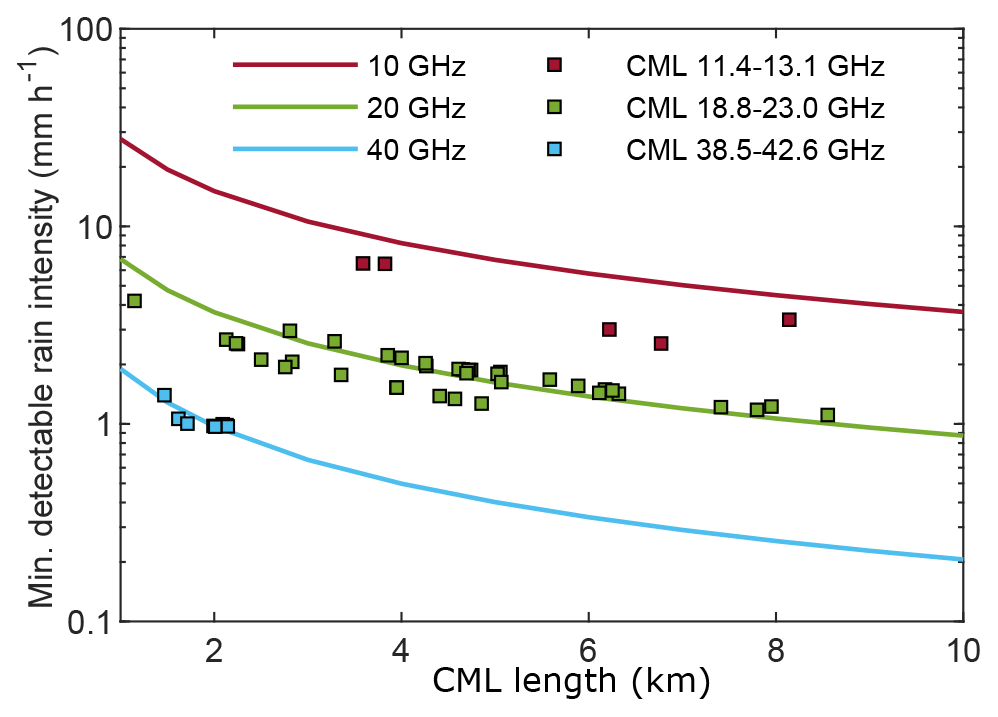
Figure 3Minimum detectable rainfall intensity as a function of path length for link frequencies of 10, 20, and 40 GHz, assuming a 1 dB quantization step on RSL. Squares represent the frequency and length of the 50 available CMLs in the study area.
In order to validate the rainfall estimates provided by CMLs, we compared the accumulated rainfall during each of the events in Table 1 with direct RG measurements. In this respect, we highlight that CMLs carry out path-averaged rainfall measurements. Hence, it is not straightforward to validate CML-based outcomes with measurements from rain gauges, which are single-point sensors, unless ad hoc deployments are used, which is not the case of this study. Here, CMLs and RGs are associated according to their mutual distance. Each RG is given a different weight depending on its position with respect to an associated CML. This is done as follows: the CML path is divided into short segments, the distance between the RG and each CML segment (approximated by its midway point) is calculated, and all of the above distances are averaged. The number coming out of this calculation accounts for the relative positions of the CML and the RG as well as the CML length. Finally, the rainfall accumulated from the set of RGs associated with a given CML is calculated with the IDW method using the average CML–RG distance. The scatter plot between CML- and RG-based accumulated rainfall is plotted in Fig. 4 for the eight high-intensity (panel a) and the four low-intensity (panel b) events. Only RGs within 5 km (average distance) of a CML are considered. During high-intensity events, there is a good match between CML and RG estimates, whereas CMLs exhibit an evident underestimation (more than 30 % on the average) in the case of low-intensity events. This pattern can be explained by the lack of sensitivity of CMLs to low rainfall intensities due to signal quantization. In Appendix A, we present a further local comparison of rainfall time series, between CMLs and nearby RGs.
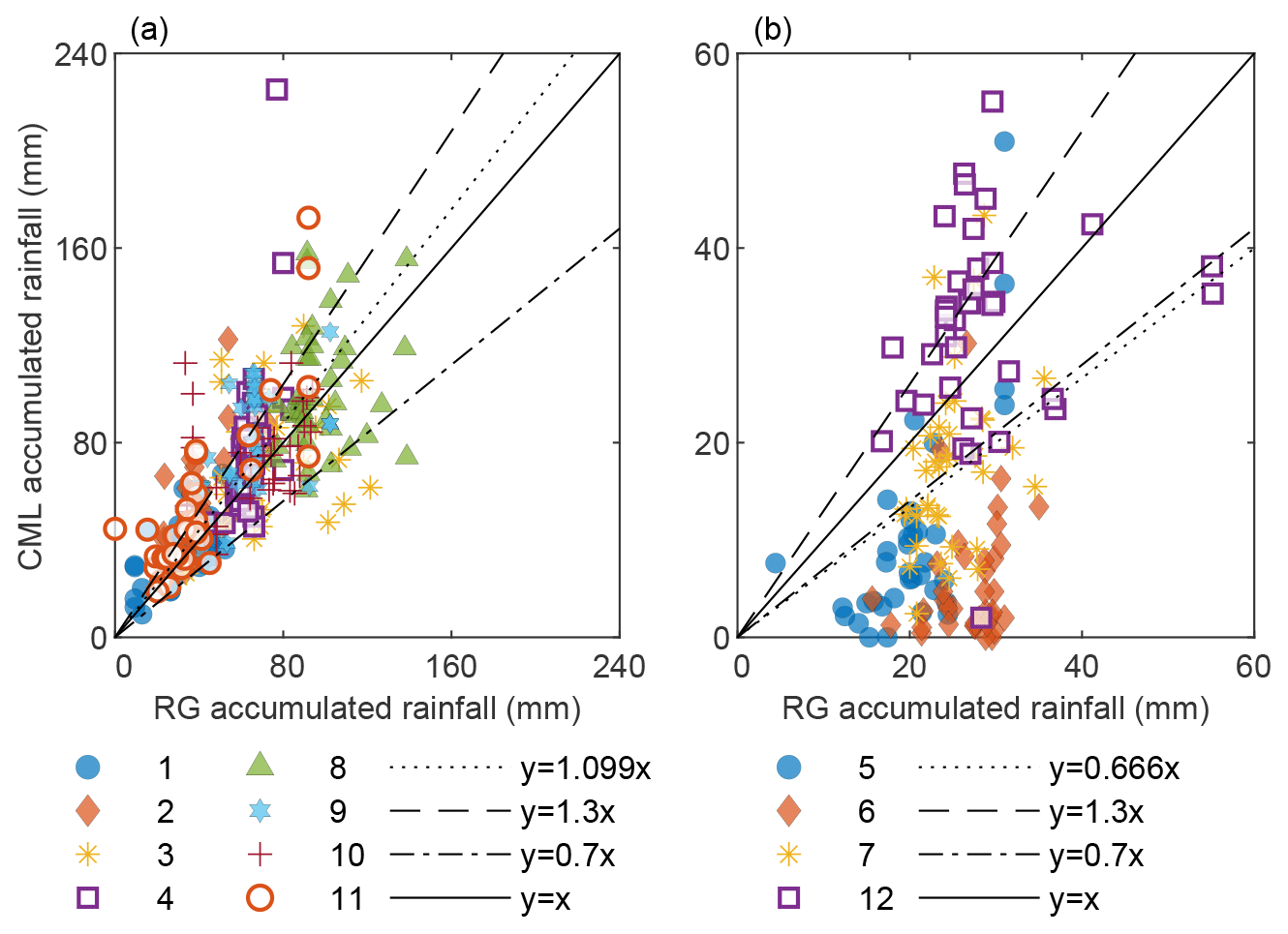
Figure 4Accumulated rainfall during (a) high-rain-rate events and (b) low-rain-rate events: CMLs against nearby RGs. The best fit of data, the ±30 % bounds, and the 45∘ line are shown as well. In the legend, numbers refer to the storm events, and markers are the selected CMLs.
3.2 Hydrological model
We used a semi-distributed rainfall–runoff model, at an hourly timescale. As shown in Fig. 1, the catchment area is divided into 15 HRUs, which are considered meteorologically, geologically, and hydrologically homogeneous. Hence, the model parameters are set at the HRU scale.
The river discharge at time t, Q(t), in HRU's outlets is calculated as the sum of two main components:
where Qs is the contribution given by the surface runoff R*, (i.e. the portion of rainfall not infiltrated into the soil), and Qg is the groundwater discharge.
The computation of R* (in mm) relies on the Soil Conservation Service curve number (SCS-CN) method (Natural Resources Conservation Service, 1985):
where P≥Ia (in mm) is the rainfall depth, S (in mm) is the maximum soil potential retention, and Ia (in mm) is the initial abstraction (calculated as a percentage, 20 %, of S). According to the United States Department of Agriculture (USDA) SCS guidelines, the soil moisture condition antecedent to a storm event is classified depending on the value of the 5-day antecedent rainfall. Here, we account for the actual soil moisture in a dynamical way, as proposed in the AnnAGNPS model (Bingner and Theurer, 2005) and also implemented in Ravazzani et al. (2007). In particular, the value of S(t) is updated as a continuous function of the degree of soil saturation ϵ(t) (-):
Here, the respective weights WI (-) and WII (-) are defined as follows:
In the above equations, SI, SII, and SIII are the retention parameters associated with the curve numbers CNI, CNII, and CNIII respectively. Finally, ϵ(t) is calculated as
where θsat (-) is the soil moisture at saturation conditions, and θres (-) is the residual soil moisture.
To calculate Qs at time t, the runoff is routed to the HRU's outlet, representing each HRU as a linear reservoir model (Dooge, 1973):
where m mm−1 is a conversion factor, r* is the surface runoff rate (in mm s−1), A (in m2) is the HRU area, and Tlag (in s) is the lag time calculated as 0.6 times the concentration time (Tc) for average natural watershed conditions and an approximately uniform distribution of runoff according to Mockus (1957) and de Simas (1996). The calculation of Tc, in each HRU, relies on the formula proposed by Ferro (2006).
The portion I (in mm) of total rainfall that infiltrates in the shallower layer of soil can either be lost by evapotranspiration, ET (in mm), or by percolation, D (in mm). Potential evapotranspiration (PET) is calculated here using the Hargreaves and Samani (1985) equation, which requires temperature data. The actual evapotranspiration (ET) is computed as a fraction of PET following Ravazzani et al. (2015). The water balance equation, referred to the shallower layer of soil with depth z (in mm) at time t, is formulated as
where θ (-) is the actual soil moisture. D(t) is the drainage flux calculated as
where (in (mm s) m−1) is a conversion factor, Ksat (in m s−1) is the hydraulic conductivity at saturation, and B is the Brooks–Corey index (Brooks and Corey, 1964). Finally, , where ΔT=3600 s. The interaction among HRUs is presented in series or in parallel reservoirs, according to the development of the river network, as exhibited in Fig. 1b. CN values were taken from https://www.isprambiente.gov.it (last access: 10 March 2022), and the θres, θsat, and B parameters were taken from Maidment (1993). Ksat and z are instead calibrated, as reported below.
Calibration and validation of the hydrological model
The hydrological model was calibrated using, as input, the hourly rainfall depths from the RG network in Fig. 1a. The chosen period for calibration is from 1 January to 31 December 2019. We tested different combinations of the two parameters, Ksat and z, and we selected the combination maximizing the Nash–Sutcliffe efficiency (NSE; Nash and Sutcliffe, 1970). Concerning Ksat, we tested the values reported in Maidment (1993) multiplied by several different powers of 10, . The values of Ksat taken from the literature are different depending on the type of soil characterizing each HRU. With regard to z, we tested all of the values inside the [10 cm, 3 m] range, with a 10 cm step. The parameter validation was carried out over two non-consecutive 6-month periods: from 1 July to 31 December 2018 and from 1 January to 30 June 2020. The NSE value is 0.69 for the calibration and 0.56 for the validation. Please note that the calibrated parameters provide an NSE larger than 0.5 for the overall 1-year validation period, which is the minimum value recommended by Moriasi et al. (2007) to consider a simulation reliable.
It is also worth noting that the calibration and validation steps were particularly troublesome due to the presence of the Cavo Diotti Dam, which artificially regulates the outflow of Pusiano Lake during flood events.
3.3 Spatial interpolation of rainfall data
Several methodologies have been proposed and applied for the spatial interpolation of rainfall measurements retrieved from CMLs (e.g. Fencl et al., 2013; Overeem et al., 2013; D'Amico et al., 2016; Haese et al., 2017; Chwala and Kunstmann, 2019; Graf et al., 2020; Eshel et al., 2021). Here, we exploited the simple and robust IDW method (Shepard, 1968) for both RG and CML measurements. According to the IDW method, given n measurements at given points xi, with i=1…n, the interpolated value u, in x, is calculated as
with
where d(xi,x) is the distance between the measuring point xi and the coordinates of the HRU's centroid x, and γ>0. The number of contributing measurements n is the number of contributing measurements within a distance dmax from the query point. We identified the appropriate value for γ and dmax by leave-one-out cross validation. We estimated the precipitation, at each RG point, from the remainder of RGs at a distance smaller than dmax, and we calculated the root-mean-square error (RMSE) between observations and estimates. The process was repeated for several values of γ and dmax. We set a minimum dmax value equal to 10 km, to have at least one neighbour available for every considered RG. To this end, we exploited a larger set of 38 RGs (including the 13 RGs in Fig. 1a) located over a wider area compared with the Lambro Catchment, and we used data from January 2018 to June 2020. The resulting RMSE distribution as a function of dmax and γ is reported in Fig. 5. We observe that the choice of dmax has a rather marginal effect on the estimates if γ≥2. The minimum RMSE is achieved when γ is slightly above 3. Therefore, we chose γ=3. Moreover, we selected dmax=10 km, which provides the best RMSE when γ=3.
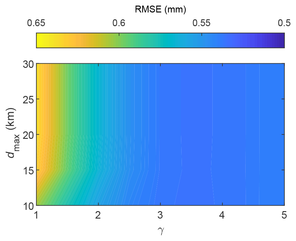
Figure 5IDW calibration based on RGs: the RMSE between observed and simulated rainfall depths, for different values of γ and dmax, from Eq. (13).
To spatially interpolate CML rain rates, we handled them as “virtual” RGs, assuming that the rainfall measurement is collapsed into the midpoint of the CML path. Again, we used the IDW method as well as the same values of γ and dmax as above. In addition to considering only RGs (or only CMLs), we accounted for the integration of RG and CML measurements. In the following, we will refer to this option as CML+RG.
The results are presented in the following two subsections. Section 4.1 provides a comparison of rainfall depths interpolated at the HRU centroids, by using data either from conventional or opportunistic sensors. Both accumulated rainfall values and hourly rainfall depths are considered at the basin and sub-basin scale, for the 12 events. Therefore, we investigate whether there are some critical issues that might help to explain differences in the rainfall–runoff model outputs. Section 4.2 analyses discharge performance by comparing RG-, CML-, and RG+CML-driven simulations with the observed flow rates.
4.1 Comparison between RG and CML rainfall data in each HRU
Figure 6 shows the scatter plot of the rainfall accumulated at the end of each of the 12 storm events and averaged over the entire catchment area. Yellow markers are CML against RG rainfall depths, and orange markers are CML+RG against RG rainfall depths. On the one hand, for all of the low-rain-rate events (squares), estimates from CMLs and from CMLs+RGs are lower than those from RGs. On the other hand, CML (and CML+RG) estimates of high-rain-rate events are in agreement (with either lower or higher values) with the RG-based estimates, with the only exception being event 3. From a more general perspective, the two regression lines indicate a good agreement between the two sets of sensors.
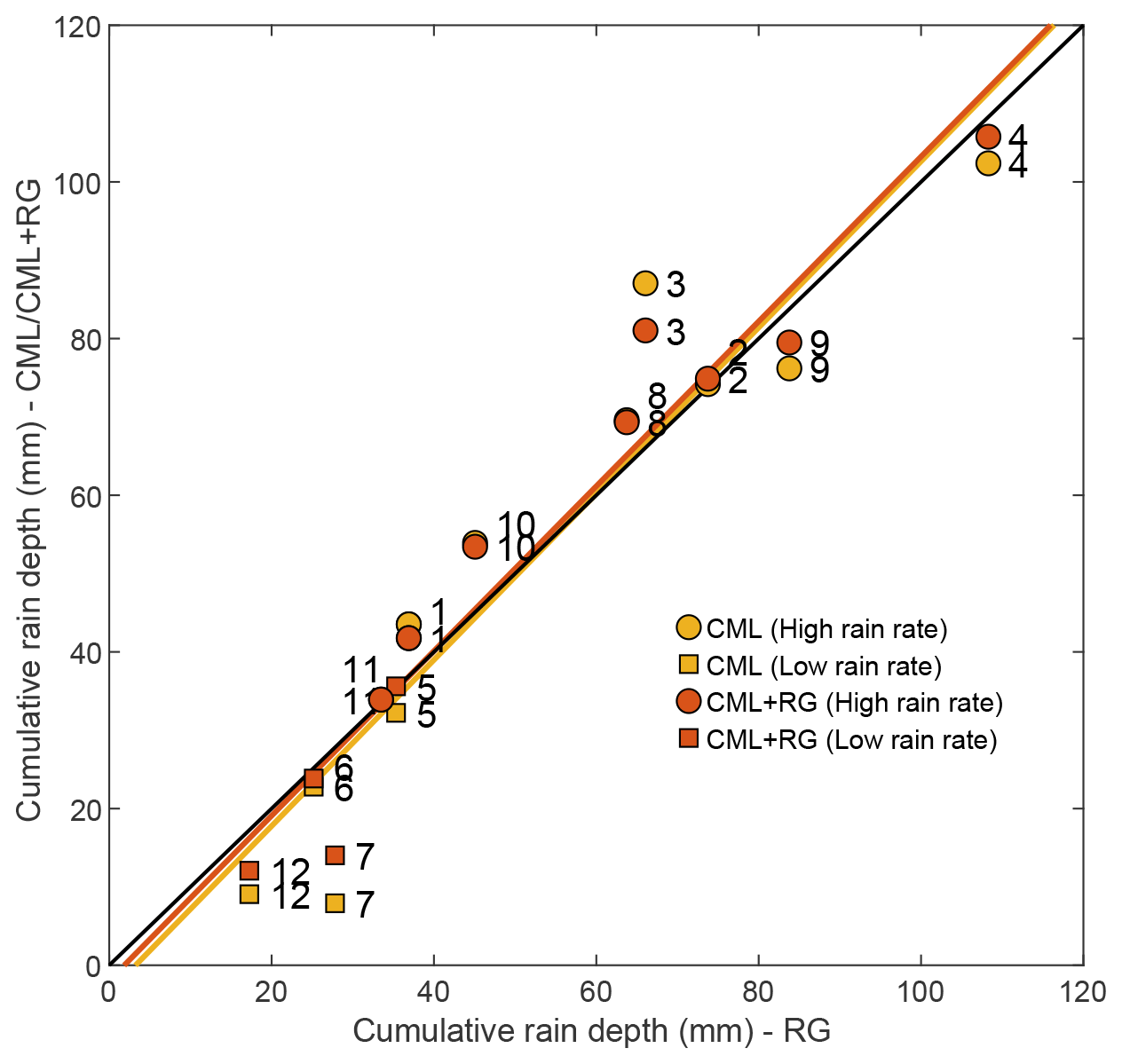
Figure 6Rainfall depths, averaged over the catchment area and accumulated at the end of each of the 12 events. The numbers next to the markers refer to the event ID, while the two different markers represent high-rain-rate (circles) and low-rain-rate (squares) events. The black line represents the 1:1 line – a perfect match between rainfall depth estimates from RGs and from CMLs (yellow) or from the combination of RGs and CMLs (orange). Yellow and orange lines are the corresponding regression lines.
We further assessed CML and RG rainfall estimates on an hourly timescale and at a sub-basin spatial scale by calculating the relative error of CML estimates with respect to RG values, assuming the latter as a benchmark, for the hourly rainfall depths inferred in the 15 HRU centroids. The relative error ΔE is evaluated as follows:
where RCML and RRG are the 1 h rainfall depths estimated in each HRU centroid from CMLs and RGs respectively. For the calculation, we only considered wet hours (RRG≥1 mm in HRU centroids), relying on a data set of 2061 values. Hence, when the CML estimate yields 0 and the RG estimate is greater than 0 (false negative), the relative error is −1. Figure 7 shows a 2D histogram representing the count of rain hours falling in a given range of RG-estimated rainfall depths and in a given range of relative errors. The increasing spread of ΔE values with respect to the decrease in the RG-based rainfall depths is due to the greater uncertainty of CMLs regarding the detection of low rain rates. If the RG-based rainfall depth is smaller than 3 mm, only 30 % of ΔE values fall in the range, whereas if it is larger than 3 mm, the percentage increases up to nearly 70 %. Moreover, for the lowest rainfall depths, there are fewer negative values of ΔE, as we set all of the CML rain rate estimates lower than the sensitivity of the link itself to zero. The high count related to and RG-based rainfall depths <5 mm is due to the occurrence of false negatives.
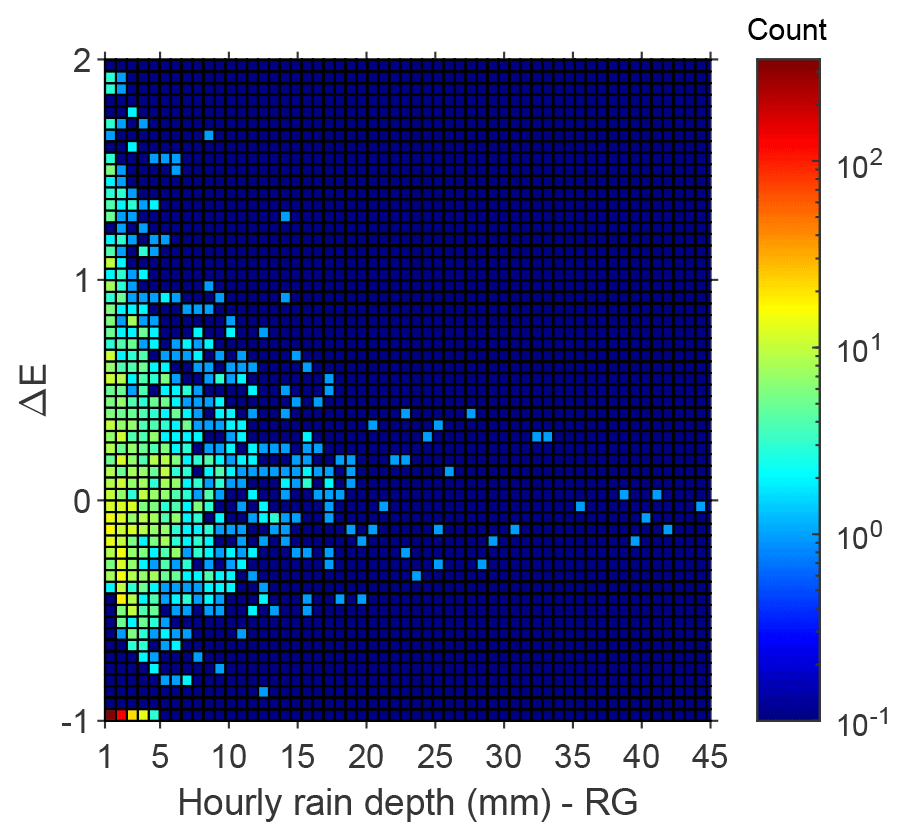
Figure 7A 2D histogram of hourly rainfall depth from RGs and ΔE. The colour of each equally spaced 2D bin represents its height, which is the count of data falling in the bin. The scale bar has a logarithmic scale, and the dark-blue bins correspond to zero counts. Values of ΔE equal to −1 represent false negatives.
Therefore, we focused on the CML hourly wet–dry classification, inferred in HRU centroids, again considering RG estimates as a benchmark. We recall that dry hours are those in which the detected rainfall depth is lower than 1 mm and vice versa for wet hours (see also Sect. 2). Figure 8 depicts box plots of the percentage of false negatives and false positives for low-rain-rate and high-rain-rate events. In contrast to a false negative, a false positive occurs when an hourly slot is classified as wet by CMLs and dry by RGs. The two box plots on the left (in Fig. 8) were obtained by relying on 120 values comprising the percentages of false positive and false negative hours in each of the eight high-rain-rate events and for each of the 15 HRUs, whereas the box plots on the right were built from 60 values comprising the percentages related to the four low-rain-rate events in each HRU. For example, the maximum percentage of false negatives is 60 %, which corresponds to HRU 2 during low-rain-rate event 7 in Table 1. From a general point of view, low-rain-rate events exhibit a higher median and a larger dispersion of false negatives than high-rain-rate events, whereas the occurrence of a false positive is relatively rare in both cases. These results confirm the inability of CMLs to detect low rain rates, which depends on the quantization error issue discussed in Sect. 3.
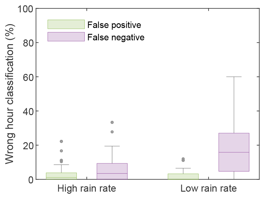
Figure 8The percentage of hours subjected to incorrect wet–dry classification (false negative or false positive), with respect to high-rain-rate and low-rain-rate events. The box plots display the median, the 0.25 (lower) and 0.75 (upper) quantiles, outliers (computed using the interquartile range), and the minimum and maximum values excluding any outliers.
Finally, in Fig. 9, we report box plots of ΔE values calculated for rainfall accumulated by each HRU over each of the 12 events. Again, the events are grouped in two classes according to rainfall intensity. The contrasting behaviour between low-rain-rate and high-rain-rate events is evident. In the former case, ΔE is mostly much lower than zero, and it is much more scattered. Once again, this result confirms that CMLs are not able to properly detect the lowest rainfall intensities during low-rain-rate events. Regarding high-rain-rate events, there is not a clear trend. The median ΔE values are always within the range, and their dispersion is low as well.
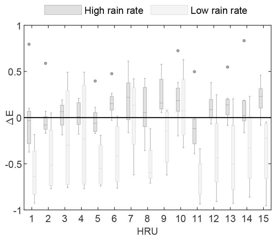
Figure 9Box plots of ΔE in each HRU for the 12 storm events (divided in two groups according to rainfall intensity). The box plots display the median, the 0.25 (lower) and 0.75 (upper) quantiles, outliers (computed using the interquartile range), and the minimum and maximum values excluding any outliers.
4.2 Comparison between RG- and CML-driven discharge simulations
In the following, discharge simulations obtained from three different data inputs (RGs, CMLs, and CMLs+RGs) are assessed and compared with hydrographic measurements at the Lesmo River section.
The output performance was evaluated using three indices: (1) the well-known Nash–Sutcliffe efficiency (NSE), (2) the relative error on peak discharge (REP), and (3) the relative error on flow volume (Dv). The last two indices are defined as follows:
In the above equations, is the simulated peak discharge, is the observed peak discharge, Vsim is the simulated total flow volume, and Vobs is the observed total flow volume.
The performance of the 12 discharge simulations, grouped by rainfall data input, is summarized in Fig. 10, using box plots. The statistical dispersion (represented by the interquartile range) of CML-based discharge simulations is larger than that of RG-based simulations. The use of CML data in the rainfall–runoff model seems to produce higher uncertainty. The combined use of RGs and CMLs instead decreases the statistical dispersion of results and leads to performance closer to that achieved with RGs. Generally, CMLs exhibit worse performance than RGs in terms of the NSE and Dv. As for REP, the two sets of sensors produce comparable errors of opposite sign; hence, their combined use leads to an optimum value of the median error (0.06).

Figure 10Panels (a) to (c) show box plots of performance metrics, namely the respective NSE, REP, and Dv, for the 12 selected flood events. The optimum values correspond to the bold black lines. The box plots display the median, the 0.25 (lower) and 0.75 (upper) quantiles, outliers (computed using the interquartile range), and the minimum and maximum values excluding any outliers.
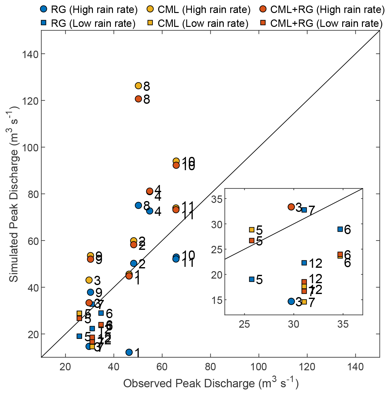
Figure 11Observed peak flow against that simulated from RG (blue), CML (yellow), and CML+RG (orange) data. The two different markers represent high-rain-rate (circles) and low-rain-rate (squares) events. The inset presents a zoomed in view of events with a low peak discharge.
To gain a deeper understanding of the model performance with respect to flow peaks, we produced a scatter plot of observed against simulated flow peaks (see Fig. 11). The scatter plot firstly reveals that the best match between observations and simulations is not always achieved by RG-based simulations. In fact, for events 1, 3, 5, and 11 the optimum match is given by CML- or CML+RG-based simulations. Moreover, the low-rain-rate events typically result in underestimated peak flow simulations with respect to the observations, considering either conventional or unconventional sensors, with the exception of event 5.
Figure 12 reports model inputs and outputs for events 5 and 2. We selected these two examples as they are characterized by a different meteorological configuration and lead to contrasting model performance. The first event is an autumn stratiform occurrence, characterized by low rain intensity. In Fig. 12a, we can see that CML-based estimates in HRUs 1, 2, 5, 8, and 11 are quite low, with respect to RGs, due to the difficulties of CMLs in detecting light rain. In contrast, in the southern HRUs (HRU 10, 12, 13, 14, and 15), which have much more influence on the generation of river discharge, CML estimates are higher than RG values. Figure 12b shows an example in which the CML-driven simulation better represents the observed outflow hydrograph, with respect to the RG-driven simulation. In particular, the best performance is gained when both types of rainfall sensors are used, and it provides an excellent Dv (equal to 0.03). The highest discrepancies between CML and RG estimates mostly involve the northern portion of the basin and have less impact on generating discharge. Event 2 is instead a typical intense convective summer occurrence, characterized by a single rainfall peak. As rain rates are high throughout the basin, contrary to event 5, we observe (as seen from Fig. 12c) a better agreement between CML and RG estimates. River discharge simulations, reported in Fig. 12d, are satisfactory, considering all three input data types. NSE values obtained from RG, CML, and RG+CML data are 0.86, 0.77, and 0.80, respectively.
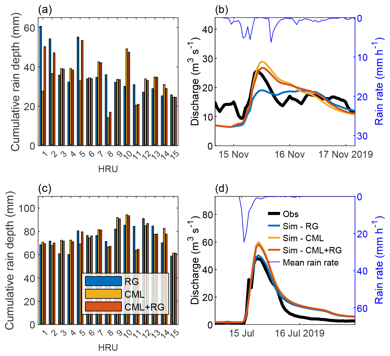
Figure 12Panels (a) and (c) show the cumulative rainfall depth estimates from RG, CML, and CML+RG for storm/flood events 5 and 2 respectively. Panels (b) and (d) present discharge observations and simulations gathered using the three different input data types, for the two same events.
As the hydrological model has been calibrated with RG-detected rainfall data, it can be assumed that the best model performance is also mostly achieved with RG data as input. Unfortunately, we did not have a database of CML events at our disposal that was large enough to carry out a CML-based calibration. Nevertheless, we tried to overcome this problem, by recalibrating model parameters, with CML and CML+RG rainfall estimates as input, relying on the 12 available flood events. Hence, the same event-based calibration was conducted using RG data as rainfall inputs. In such a way, the comparison on discharge simulations may be led in a fair manner. We considered parameters providing the highest median NSE values as the optimum parameters. Performance indices, subdivided by the type of rainfall data input and the type of calibration, are summarized using box plots in Fig. 13. Please note that CML- and CML+RG-based calibrations improve the performance of the model when fed by unconventional input data. In particular, NSE values are comparable with those achieved by the use of RG data with an RG-based calibration. In fact, median NSE values for RG inputs with RG-based calibration, CML inputs with CML-based calibration, and CML+RG inputs with CML+RG-based calibration are 0.37, 0.35, and 0.38 respectively. For REP values, we generally observe underestimations of the observed peak flow, considering CML- and CML+RG calibration but a smaller interquartile range when compared with RG-based calibration. Concerning Dv values, performance for the CML- and CML+RG-based calibration is quite satisfactory, despite the fact that the combination providing the best performance is still RG inputs with RG-based calibration.
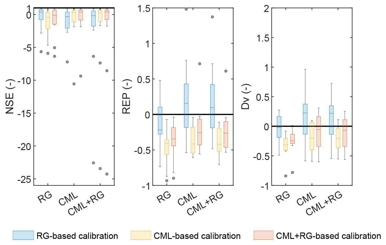
Figure 13Box plots of the performance indices for the 12 flood events obtained with three different calibration sets (drawn in as many colours) and with three different input types (on the x axis). The box plots display the median, the 0.25 (lower) and 0.75 (upper) quantiles, outliers (computed using the interquartile range), and the minimum and maximum values excluding any outliers.
The analysis of interpolated rainfall data carried out in Sect. 4.1 reveals that CML and RG estimates of accumulated areal-averaged rainfall depths are comparable. However, two issues emerged.
First, CMLs exhibit a different behaviour depending on the event intensity, as their sensitivity varies with length and frequency. Specifically, they return lower values of rainfall depth and rainfall accumulation in connection with low-rain-rate events. This aspect becomes evident at either different spatial scales (sub-basin and basin scales) or different temporal scales (hourly and event-based timescales). In fact, due to a coarse quantization of the raw data, CMLs are not sensitive to low rain intensity; hence, when the rainfall depth value over a certain lapse of time is required (in our case 1 h), this limitation may lead to large errors, especially when light rain goes on for a long time. Despite some discrepancies in the behaviour of single CMLs with respect to their nearby RGs, as highlighted in Appendix A, we observed a good agreement between CML- and RG-based estimates in HRU centroids for high rain rates due to spatial interpolation which could mitigate such biases.
The second issue is the different CML density over the HRUs. It is well known that spatial interpolation methods are sensitive to sensor density (Xu et al., 2013); consequently, the relatively large distance of the available CMLs from the HRU centroids in the most scarcely populated areas (northern HRUs) may lead to a loss of reliability in the estimated rainfall depths. However, such an aspect appears to be less relevant when compared with the first issue outlined above, at least when dealing with quite large HRUs (dozens of square kilometres). In fact, a careful comparison of Figs. 2 and 9 does not show an evident correlation between the mean CML–centroid distances and ΔE values.
Last but not least, model performance is influenced by the calibration process of model parameters. Similar model performance, in terms of the NSE index, can be achieved with all three types of input data (RGs, CMLs, and CMLs+RGs) if the calibration is carried out with the respective data inputs. This means that, after a proper calibration, opportunistic sensors could be exploited in semi-distributed hydrological models, as well as RGs. In particular we found that, after calibration, the RGs+CMLs data set provides the highest median NSE. However, it is worth highlighting that we calibrated the parameters on the basis of only 12 flood events. In order to assess a robust calibration and the associated validation, a larger data set of CML-based rainfall events should be processed.
5.1 Limitations and improvements
One of the major difficulties encountered during analyses was the small amount of CML data, as we relied on only 458 h of CML raw data grouped in 12 events. On the other hand, the database of RG observations was much wider, and we disposed of real-time data. An extension of the CML-based data set of events or, better yet, access to real-time CML raw data would definitely greatly benefit the present work. Firstly, it would allow for the development of a more robust statistical analysis of storm/flood events. Secondly, it would enable a proper calibration and a validation of the hydrological model based on CML data as rainfall input.
To enhance this work, it would also be useful to resort to the implementation of a CML-driven distributed model, which is expected to provide a more accurate description of the spatial variability in the precipitation field compared with a semi-distributed model. In such a case, the CML measurements would be better exploited by the use of advanced methods for the spatial reconstruction of the rainfall field. For instance, techniques such as the tomographic reconstruction algorithm (D'Amico et al., 2016) or the stochastic reconstruction based on copulas (Haese et al., 2017; Salvadori et al., 2007) take advantage of the path-integrated nature of CML measurements.
5.2 CML operational platforms
Although we showed that CML rainfall data can be successfully assimilated into hydrological models, their integration into real-time operational platforms (e.g. early-warning systems) remains challenging. A number of aspects should be still considered including the following:
-
generation of CML raw data formats suitable for rainfall estimation;
-
real-time collection of raw data, which should be transparent to network operation;
-
data transfer to a control centre;
-
non-trivial data reduction process, especially if large sets of CMLs are managed.
The above-mentioned issues suggest a systematic cooperation with mobile operators, who are the owners of CML network infrastructure.
5.3 New insights on the areal reduction factor
To this point, we have mainly investigated the exploitation of CML-based rainfall estimates with the purpose of testing their impact on the hydrological simulations of river discharge, with respect to the use of RG data. However, other important hydrological issues could be addressed by dealing with CML data. One such issue is definitely the modelling of the areal reduction factor (ARF): the factor that transforms a point rainfall for a given duration and return period into the areal average value for the same duration and return period (Natural Environmental Research Council, 1975). Over the last few decades, great efforts have been devoted to modelling the ARF (De Michele et al., 2001), which is useful for the design of hydraulic and hydrological infrastructures, for flood risk evaluations, and for rainfall threshold estimations in early-warning systems (e.g. Kim et al., 2019; Biondi et al., 2021). As we dealt with a semi-distributed hydrological model, we needed to transform point (from RG) and linear (from CML) precipitation measurements into areal values, over the HRU areas. Therefore, from a different perspective, this work could also be seen as a first step in order to test the modelling of the ARF using a combination of conventional and unconventional sensors.
In this work, we assessed the use of commercial microwave links (CMLs) as opportunistic rainfall sensors within hydrological modelling. We focused on Lambro, a peri-urban catchment, 260 km2 in area, located north of Milan (Italy) and covered by 50 CMLs that are part of the network owned by a major mobile operator. The Lambro Catchment area is also covered by 13 rain gauges (RGs), which we used both as an independent rainfall data set and in combination with CMLs. We implemented a semi-distributed hydrological model and carried out two types of comparison between CML and RG data. First, we considered rainfall data (hourly rainfall depths, the input of the hydrological model, and total accumulations at the storm end, for a sample of 12 storm events) interpolated at the HRU centroids. We then compared river discharge simulations (model output) from RGs, CMLs, and RGs+CMLs against flow measurements.
Concerning the comparison of the two sources of rainfall data, we found that high-intensity events detected by CMLs are in accordance with RG measurements. On the other hand, we came across a critical aspect with respect to the inability of CMLs to detect low rain rates, due to the coarse 1 dB quantization step of raw data (i.e. received power levels). The minimum detectable rainfall intensity depends on the operation frequency of CMLs as well as on their length; for the available set of CMLs, the minimum detectable rainfall intensity ranges from 1 to 10 mm h−1. Such a limitation results in the underestimation of rainfall depths interpolated in the HRU centroids for low-intensity storm events, when compared with RG-based rainfall data.
The hydrographs simulated by the hydrological model perform better in terms of the Nash–Sutcliffe efficiency (NSE) and relative error on flow volume (Dv) in the case of RGs compared with CMLs. This result is not surprising, as the model was calibrated using RG data for 1 year. Nevertheless, satisfactory values of relative error on peak discharge (REP) are achieved through the use of CML and CML+RG data as inputs to the RG-based calibrated model.
By calibrating the model with CML data and by using the same as input, it is possible to improve the model performance, which becomes comparable with the case of RG calibration and RG input. Even a slightly better performance can be gathered with a CML+RG-based calibration and CML+RG data as input.
Despite the lack of sensitivity of the CMLs that we relied on, this analysis proves that rainfall estimates based on CMLs could be exploited in hydrology, with a certain confidence, for river discharge simulations. These results show that the use of opportunistic sensors could support hydrological modelling, especially in areas lacking traditional monitoring systems. Furthermore, in the regions already equipped with traditional rainfall sensors, the integration of existing instrumentation with CMLs could also provide advantages for hydrological applications, as this increases the number of reliable rainfall measurements.
Here, rainfall amounts collected from CMLs and RGs are compared via an analysis of the corresponding time series. To this end, we selected four CMLs that had at least one RG within 5 km, as done for the scatter plots in Fig. 4, and we plotted the CML and RG time series of rainfall intensity and cumulative rainfall depth during storm events 7, 8, 9 and 10 in Table 1. Please note that rainfall intensity is obtained from slightly different time resolutions (i.e. 15 min for CMLs and 10 min for RGs). Figure A1 shows the results. The differences between individual CMLs and nearby RGs are not surprising and are due to three main factors: (1) the different nature of the sensors; (2) the fact that CMLs were not calibrated using other rainfall sensors, such as weather radars; and (3) the relative position between the CMLs and RGs. What is mostly evident is the difference between the low- (event 7) and high-intensity events (events 8, 9, and 10). In the former case, the CMLs miss most of rainfall occurrences, causing a large underestimation of the rainfall accumulated at the end of the event. During event 7, RGs detected rain intensities from 1 up to 6 mm h−1. The last value is approximately the minimum detectable rain intensity for the CML with lowest frequencies (in Fig. A1a). However, it is worth emphasizing that such underestimating behaviour is observable not only for short and low-frequency CMLs but also for the most sensitive ones. In fact, large underestimations are reported in Fig. A1g, l, and q, which are related to links with a minimum detectable rain intensity of 1.6, 1.4, and 1 mm h−1 respectively. This systematic underestimation also impacts estimates of rainfall depths at the basin and sub-basin scale, as shown by the results in Sect. 4.1. The three high-rain-rate events highlight different behaviours depending on the CML considered and its relative location with respect to the RGs. The short and low-frequency CML, given in Fig. A1a, shows quite a large discrepancy with its nearby RG with respect to either the peak's timing or the total observed rainfall depth, and it reveals both underestimating and overestimating behaviour (Fig. A1c, e). The performance of the two medium-length and medium-frequency CMLs (Fig. A1h–j and m–o) is in mutual agreement and is definitely better with respect to the case shown in Fig. A1c–e. Specifically, it can be noticed that, in most of the cases, these two CMLs successfully reproduce the highest peaks observed by the closest RGs, which are also those located right next to their middle point. However, they show some discrepancies (lower values with respect to RGs) as the rain rate decreases. This behaviour is particularly evident in Fig. A1i and n for event 9. Finally, the highest-frequency CML exhibits different performance during the three high-rain-rate events (Fig. A1r–t). For example, at odds with the previous cases, in event 10, the CML tends to overestimate the lowest rain rates, leading to a large overestimation (up to 60 %) of the cumulated rainfall depth. In this case, the differences between the CMLs and RGs could also be due to the non-optimal relative location between the CMLs and RGs. The results reported in Sect. 4.1 show that interpolating several CML data at HRU centroids mitigates the inaccuracy of individual CMLs and leads to acceptable estimates of the flow except in the case of low-intensity events due to their limited sensitivity.
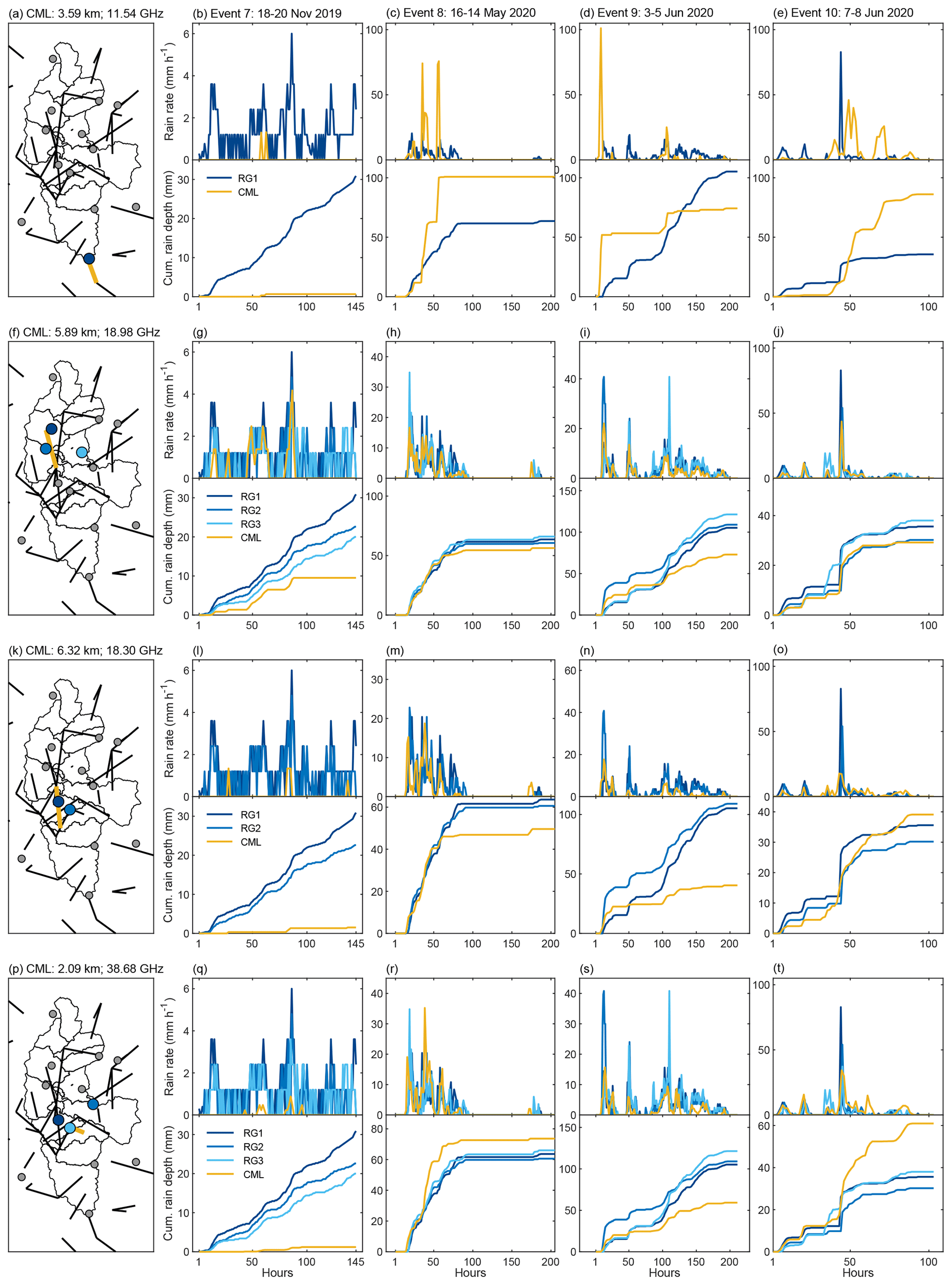
Figure A1Comparison between single CMLs and their nearby RGs. Each row shows (1) the location of the selected CML in the Lambro Basin and its nearby RGs, (2) the CML–RGs comparison with respect to the rain rate time series, and (3) the CML–RGs comparison with respect to the cumulated rainfall depths.
Meteorological and hydrological data from the Hydrographic Office of ARPA Lombardia are openly available at https://www.arpalombardia.it/Pages/Meteorologia/Richiesta-dati-misurati.aspx (Rete Regionale di Rilevamento Meteorologico di ARPA Lombardia, 2022). Commercial microwave link data are available from the authors with the permission of Vodafone Italia S.p.A.
CDM, RN, MDA, and AG conceptualized the study. RN handled the CML data. GC handled the gauge data. GC, CD, and CDM developed the hydrological model. GC carried out the model calibrations and validations. GC prepared Figs. 1–2, 5–13, and A1, and RN prepared Figs. 3 and 4. GC wrote the first draft of the paper, and all of the authors reviewed the paper.
At least one of the (co-)authors is a member of the editorial board of Hydrology and Earth System Sciences. The peer-review process was guided by an independent editor, and the authors also have no other competing interests to declare.
Publisher's note: Copernicus Publications remains neutral with regard to jurisdictional claims in published maps and institutional affiliations.
The authors wish to acknowledge support from the Fondazione Cariplo within the framework of the MOPRAM project (http://www.mopram.it, last access: 10 March 2022). We are also grateful to ARPA Lombardia for providing us with meteorological and hydrological data.
This research has been supported by the Fondazione Cariplo (grant no. 2016-0777).
This paper was edited by Matjaz Mikos and reviewed by Geoff Pegram and one anonymous referee.
Alberoni, P., Andersson, T., Mezzasalma, P., Michelson, D., and Nanni, S.: Use of the vertical reflectivity profile for identification of anomalous propagation, Meteorol. Appl., 8, 257–266, https://doi.org/10.1017/S1350482701003012, 2001. a
Arnaud, P., Lavabre, J., Fouchier, C., Diss, S., and Javelle, P.: Sensitivity of hydrological models to uncertainty in rainfall input, Hydrolog. Sci. J., 56, 397–410, https://doi.org/10.1080/02626667.2011.563742, 2011. a
Atlas, D. and Ulbrich, C. W.: Path-and area-integrated rainfall measurement by microwave attenuation in the 1–3 cm band, J. Appl. Meteorol. Clim., 16, 1322–1331, https://doi.org/10.1175/1520-0450(1977)016<1322:PAAIRM>2.0.CO;2, 1977. a
Bárdossy, A. and Das, T.: Influence of rainfall observation network on model calibration and application, Hydrol. Earth Syst. Sci., 12, 77–89, https://doi.org/10.5194/hess-12-77-2008, 2008. a
Bengtsson, L.: Daily and hourly rainfall distribution in space and time–conditions in southern Sweden, Hydrol. Res., 42, 86–94, https://doi.org/10.2166/nh.2011.080b, 2011. a
Bingner, R. L., Theurer, F. D., and Yuan, Y.: AnnAGNPS technical processes, Tech. rep., US Dept Agriculture, Agricultural Research Services, https://www.nrcs.usda.gov/wps/portal/nrcs/detailfull/national/water/quality/?&cid=stelprdb1043591 (last access: 26 April 2022), 2005. a
Biondi, D., Greco, A., and De Luca, D. L.: Fixed-area vs. storm-centered Areal Reduction factors: a Mediterranean case study, J. Hydrol., 595, 125654, https://doi.org/10.1016/j.jhydrol.2020.125654, 2021. a
Brauer, C. C., Overeem, A., Leijnse, H., and Uijlenhoet, R.: The effect of differences between rainfall measurement techniques on groundwater and discharge simulations in a lowland catchment, Hydrol. Process., 30, 3885–3900, https://doi.org/10.1002/hyp.10898, 2016. a
Brooks, R. H. and Corey, A. T.: Hydraulic properties of porous media, Fort Collins, Colorado State University, CO, USA, 1964. a
Chen, D., Ou, T., Gong, L., Xu, C.-Y., Li, W., Ho, C.-H., and Qian, W.: Spatial interpolation of daily precipitation in China: 1951–2005, Adv. Atmos. Sci., 27, 1221–1232, https://doi.org/10.1007/s00376-010-9151-y, 2010. a
Chen, J.-Y., Trömel, S., Ryzhkov, A., and Simmer, C.: Assessing the benefits of specific attenuation for quantitative precipitation estimation with a C-band radar network, J. Hydrometeorol., 22, 2617–2631, https://doi.org/10.1175/JHM-D-20-0299.1, 2021. a
Chwala, C. and Kunstmann, H.: Commercial microwave link networks for rainfall observation: Assessment of the current status and future challenges, WIRes Water, 6, e1337, https://doi.org/10.1002/wat2.1337, 2019. a
Cugerone, K. and De Michele, C.: Johnson SB as general functional form for raindrop size distribution, Water Resour. Res., 51, 6276–6289, https://doi.org/10.1002/2014WR016484, 2015. a
Dawdy, D. R. and Bergmann, J. M.: Effect of rainfall variability on streamflow simulation, Water Resour. Res., 5, 958–966, https://doi.org/10.1029/WR005i005p00958, 1969. a
De Michele, C., Kottegoda, N. T., and Rosso, R.: The derivation of areal reduction factor of storm rainfall from its scaling properties, Water Resour. Res., 37, 3247–3252, https://doi.org/10.1029/2001WR000346, 2001. a
de Simas, M. J. C.: Lag-time characteristics in small watersheds in the United States, UMI, Ann Arbor, MI, USA, 1996. a
Delhomme, J. P.: Kriging in the hydrosciences, Adv. Water Resour., 1, 251–266, https://doi.org/10.1016/0309-1708(78)90039-8, 1978. a
Dooge, J.: Linear theory of hydrologic systems, 1468, Agricultural Research Service, US Department of Agriculture, 1973. a
D'Amico, M., Manzoni, A., and Solazzi, G. L.: Use of operational microwave link measurements for the tomographic reconstruction of 2-D maps of accumulated rainfall, IEEE Geosci. Remote S., 13, 1827–1831, https://doi.org/10.1109/LGRS.2016.2614326, 2016. a, b
Eshel, A., Messer, H., Kunstmann, H., Alpert, P., and Chwala, C.: Quantitative analysis of the performance of spatial interpolation methods for rainfall estimation using commercial microwave links, J. Hydrometeorol., 22, 831–843, https://doi.org/10.1175/JHM-D-20-0164.1, 2021. a
EU Water Directors: Best Practices on flood prevention, protection and mitigation, Meetings, Budapest, 30 November and 1 December 2002, Bonn, 5 and 6 February 2003, http://ec.europa.eu/environment/water/flood_risk/pdf/flooding_bestpractice.pdf (last access: 10 March 2022), 2003. a
Fencl, M., Rieckermann, J., Schleiss, M., Stránskỳ, D., and Bareš, V.: Assessing the potential of using telecommunication microwave links in urban drainage modelling, Water Sci. Technol., 68, 1810–1818, https://doi.org/10.2166/wst.2013.429, 2013. a, b
Fenicia, F., Pfister, L., Kavetski, D., Matgen, P., Iffly, J.-F., Hoffmann, L., and Uijlenhoet, R.: Microwave links for rainfall estimation in an urban environment: Insights from an experimental setup in Luxembourg-City, J. Hydrol., 464–465, 69–78, https://doi.org/10.1016/j.jhydrol.2012.06.047, 2012. a
Ferro, V.: Riqualificazione ambientale dei corsi d'acqua, in: Quaderni di Idronomia Montana, Nuova Editoriale Bios, http://hdl.handle.net/10447/12539 (last access: 26 April 2022), 2006. a
Giuli, D., Toccafondi, A., Gentili, G. B., and Freni, A.: Tomographic reconstruction of rainfall fields through microwave attenuation measurements, J. Appl. Meteorol. Clim., 30, 1323–1340, https://doi.org/10.1175/1520-0450(1991)030<1323:TRORFT>2.0.CO;2, 1991. a
Graf, M., Chwala, C., Polz, J., and Kunstmann, H.: Rainfall estimation from a German-wide commercial microwave link network: optimized processing and validation for 1 year of data, Hydrol. Earth Syst. Sci., 24, 2931–2950, https://doi.org/10.5194/hess-24-2931-2020, 2020. a
Haese, B., Hörning, S., Chwala, C., Bárdossy, A., Schalge, B., and Kunstmann, H.: Stochastic reconstruction and interpolation of precipitation fields using combined information of commercial microwave links and rain gauges, Water Resour. Res., 53, 10740–10756, https://doi.org/10.1002/2017WR021015, 2017. a, b
Hargreaves, G. H. and Samani, Z. A.: Reference crop evapotranspiration from temperature, Appl. Eng. Agric., 1, 96–99, https://doi.org/10.13031/2013.26773, 1985. a
Ignaccolo, M. and De Michele, C.: One, No One, and One Hundred Thousand: The Paradigm of the Z–R Relationship, J. Hydrometeorol., 21, 1161–1169, https://doi.org/10.1175/JHM-D-19-0177.1, 2020. a
ITU-R P.838-3: Specific attenuation model for rain for use in prediction methods, Tech. rep., (Recommendation P.838-3), https://www.itu.int/rec/R-REC-P.838-3-200503-I/en (last access: 26 April 2022), 2005. a
Jaffrain, J., Studzinski, A., and Berne, A.: A network of disdrometers to quantify the small-scale variability of the raindrop size distribution, Water Resour. Res., 47, W00H06, https://doi.org/10.1029/2010WR009872, 2011. a
Jameson, A. R. and Kostinski, A.: Spurious power–law relations among rainfall and radar parameters, Q. J. Roy. Meteor. Soc., 128, 2045–2058, https://doi.org/10.1256/003590002320603520, 2002. a
Kidd, C. and Huffman, G.: Global precipitation measurement, Meteorol. Appl., 18, 334–353, https://doi.org/10.1002/met.284, 2011. a
Kim, J., Lee, J., Kim, D., and Kang, B.: The role of rainfall spatial variability in estimating areal reduction factors, J. Hydrol., 568, 416–426, https://doi.org/10.1016/j.jhydrol.2018.11.014, 2019. a
Köppen, W. P.: Die Klimate der Erde: Grundriss der Klimakunde, Geogr. J., 65, ISBN-13 978-3111125107, 1925. a
Lombardi, G., Ceppi, A., Ravazzani, G., Davolio, S., and Mancini, M.: From Deterministic to Probabilistic Forecasts: The “Shift-Target” Approach in the Milan Urban Area (Northern Italy), Geosciences, 8, 181, https://doi.org/10.3390/geosciences8050181, 2018. a
Luini, L., Roveda, G., Zaffaroni, M., Costa, M., and Riva, C.: The Impact of Rain on Short E-Band Radio Links for 5G Mobile Systems: Experimental Results and Prediction Models, IEEE T. Antenn. Propag., 68, 3124–3134, https://doi.org/10.1109/TAP.2019.2957116, 2020. a
Maidment, D.: Handbook of hydrology, McGraw-Hill, New York, NY, USA, ISBN-13: 978-0070397323, 1993. a, b
Marshall, J. S. and Palmer, W. M.: The distribution of raindrops with size, J. Meteorol., 5, 165–166, https://doi.org/10.1175/1520-0469(1948)005<0165:TDORWS>2.0.CO;2, 1948. a
Masseroni, D., Cislaghi, A., Camici, S., Massari, C., and Brocca, L.: A reliable rainfall–runoff model for flood forecasting: review and application to a semi-urbanized watershed at high flood risk in Italy, Hydrol. Res., 48, 726–740, https://doi.org/10.2166/nh.2016.037, 2017. a
Messer, H., Zinevich, A., and Alpert, P.: Environmental monitoring by wireless communication networks, Science, 312, 713, https://doi.org/10.1126/science.1120034, 2006. a
Met Office: Fact Sheet No. 3: Water in the Atmosphere, Tech. rep., https://www.metoffice.gov.uk/research/library-and-archive/publications/factsheets (last access: 26 April 2022), 2007. a
Mockus, V.: Use of storm and watershed characteristics in synthetic unit hydrograph analysis and application, US Soil Conservation Service, 1957. a
Moriasi, D. N., Arnold, J. G., Van Liew, M. W., Bingner, R. L., Harmel, R. D., and Veith, T. L.: Model evaluation guidelines for systematic quantification of accuracy in watershed simulations, T. ASABE, 50, 885–900, https://doi.org/10.13031/2013.23153, 2007. a
Myers, D. E.: Co-kriging–New developments, in: Geostatistics for natural resources characterization, Springer, 295–305, 1984. a
Nash, J. E. and Sutcliffe, J. V.: River flow forecasting through conceptual models part I – A discussion of principles, J. Hydrol., 10, 282–290, https://doi.org/10.1016/0022-1694(70)90255-6, 1970. a
Natural Environmental Research Council (NERC): Flood studies report, vol. II, Tech. rep., Meteorological studies, Swindon, England, 1975. a
Natural Resources Conservation Service (NRCS): National Engineering Handbook, Part 630 Hydrology, 210–VI–NEH, US Department of Agriculture, Washington, DC, USA, https://www.nrcs.usda.gov/wps/portal/nrcs/detailfull/national/water/manage/hydrology/?cid=stelprdb1043063 (last access: 26 April 2022), 1985. a
Nebuloni, R., D'Amico, M., Cazzaniga, G., and De Michele, C.: On the Use of Minimum and Maximum Attenuation for Retrieving Rainfall Intensity Through Commercial Microwave Links, URSI Radio Sci. Lett., 2, 1–4, https://www.ursi.org/Publications/RadioScienceLetters/Volume2/RSL20-0062-final.pdf (last access: 26 April 2022), 2020. a
New, M., Todd, M., Hulme, M., and Jones, P.: Precipitation measurements and trends in the twentieth century, Int. J. Climatol., 21, 1889–1922, https://doi.org/10.1002/joc.680, 2001. a
Obled, C., Wendling, J., and Beven, K.: The sensitivity of hydrological models to spatial rainfall patterns: an evaluation using observed data, J. Hydrol., 159, 305–333, https://doi.org/10.1016/0022-1694(94)90263-1, 1994. a
Overeem, A., Leijnse, H., and Uijlenhoet, R.: Country-wide rainfall maps from cellular communication networks, P. Natl. Acad. Sci. USA, 110, 2741–2745, https://doi.org/10.1073/pnas.1217961110, 2013. a
Overeem, A., Leijnse, H., and Uijlenhoet, R.: Retrieval algorithm for rainfall mapping from microwave links in a cellular communication network, Atmos. Meas. Tech., 9, 2425–2444, https://doi.org/10.5194/amt-9-2425-2016, 2016. a, b
Parkes, B., Wetterhall, F., Pappenberger, F., He, Y., Malamud, B., and Cloke, H.: Assessment of a 1 h gridded precipitation dataset to drive a hydrological model: a case study of the summer 2007 floods in the Upper Severn, UK, Hydrol. Res., 44, 89–105, https://doi.org/10.2166/nh.2011.025, 2013. a
Pastorek, J., Fencl, M., Rieckermann, J., and Bareš, V.: Commercial microwave links for urban drainage modelling: The effect of link characteristics and their position on runoff simulations, J. Environ. Manage., 251, 109522, https://doi.org/10.1016/j.jenvman.2019.109522, 2019. a
Raghavan, S.: Radar Meteorology, Springer, ISBN-13: 978-9048164165, 2013. a
Rahimi, A., Holt, A., Upton, G., and Cummings, R.: Use of dual-frequency microwave links for measuring path-averaged rainfall, J. Geophys. Res.-Atmos., 108, 4467, https://doi.org/10.1029/2002JD003202, 2003. a
Rauber, R. M. and Nesbitt, S. W.: Radar meteorology: A first course, John Wiley & Sons, Glasgow, UK, ISBN-13: 978-1118432624, 2018. a
Ravazzani, G., Mancini, M., Giudici, I., and Amadio, P.: Effects of soil moisture parameterization on a real-time flood forecasting system based on rainfall thresholds, in: Quantification and Reduction of Predictive Uncertainty for Sustainable Water Resources Management, in: Proc. Symposium HS 2004 at IUGG 2007, IAHS Publ., Perugia, 407–416, July 2007. a
Ravazzani, G., Bocchiola, D., Groppelli, B., Soncini, A., Rulli, M. C., Colombo, F., Mancini, M., and Rosso, R.: Continuous streamflow simulation for index flood estimation in an Alpine basin of northern Italy, Hydrolog. Sci. J., 60, 1013–1025, https://doi.org/10.1080/02626667.2014.916405, 2015. a
Ravazzani, G., Amengual, A., Ceppi, A., Homar, V., Romero, R., Lombardi, G., and Mancini, M.: Potentialities of ensemble strategies for flood forecasting over the Milano urban area, J. Hydrol., 539, 237–253, https://doi.org/10.1016/j.jhydrol.2016.05.023, 2016. a
Rete Regionale di Rilevamento Meteorologico di ARPA Lombardia: Archivio dati idro-nivo-meteorologici (hydro-nivo-meteorological data archive), https://www.arpalombardia.it/Pages/Meteorologia/Richiesta-dati-misurati.aspx, last access: 10 March 2022. a
Roversi, G., Alberoni, P. P., Fornasiero, A., and Porcù, F.: Commercial microwave links as a tool for operational rainfall monitoring in Northern Italy, Atmos. Meas. Tech., 13, 5779–5797, https://doi.org/10.5194/amt-13-5779-2020, 2020. a
Salvadori, G., De Michele, C., Kottegoda, N. T., and Rosso, R.: Extremes in nature: an approach using copulas, vol. 56, Springer, Dordrecht, the Netherlands, ISBN-13: 978-9401782753, 2007. a
Schleiss, M. and Berne, A.: Identification of dry and rainy periods using telecommunication microwave links, IEEE Geosci. Remote S., 7, 611–615, 2010. a
Schleiss, M., Rieckermann, J., and Berne, A.: Quantification and modeling of wet-antenna attenuation for commercial microwave links, IEEE Geosci. Remote S., 10, 1195–1199, 2013. a
Shepard, D.: A two-dimensional interpolation function for irregularly-spaced data, in: Proceedings of the 1968 23rd ACM national conference, ACM, New York, NY, USA, 517–524, https://doi.org/10.1145/800186.810616, January 1968. a, b
Smiatek, G., Keis, F., Chwala, C., Fersch, B., and Kunstmann, H.: Potential of commercial microwave link network derived rainfall for river runoff simulations, Environ. Res. Lett., 12, 034026, https://doi.org/10.1088/1748-9326/aa5f46, 2017. a
Stransky, D., Fencl, M., and Bares, V.: Runoff prediction using rainfall data from microwave links: Tabor case study, Water Sci. Technol., 2017, 351–359, https://doi.org/10.2166/wst.2018.149, 2018. a
Thiessen, A. H.: Precipitation averages for large areas, Mon. Weather Rev., 39, 1082–1089, https://doi.org/10.1175/1520-0493(1911)39<1082b:PAFLA>2.0.CO;2, 1911. a
Xie, P., Rudolf, B., Schneider, U., and Arkin, P. A.: Gauge-based monthly analysis of global land precipitation from 1971 to 1994, J. Geophys. Res.-Atmos., 101, 19023–19034, https://doi.org/10.1029/96JD01553, 1996. a
Xu, H., Xu, C.-Y., Chen, H., Zhang, Z., and Li, L.: Assessing the influence of rain gauge density and distribution on hydrological model performance in a humid region of China, J. Hydrol., 505, 1–12, https://doi.org/10.1016/j.jhydrol.2013.09.004, 2013. a, b
Younger, P. M., Freer, J. E., and Beven, K. J.: Detecting the effects of spatial variability of rainfall on hydrological modelling within an uncertainty analysis framework, Hydrol. Process., 23, 1988–2003, https://doi.org/10.1002/hyp.7341, 2009. a
Zhang, G., Mahale, V. N., Putnam, B. J., Qi, Y., Cao, Q., Byrd, A. D., Bukovcic, P., Zrnic, D. S., Gao, J., Xue, M., Jung, Y., Reeves, H. D., Heinselman, P. L., Ryzhkov, A., Palmer, R. D., Zhang, P., Weber, M., Mcfarquhar, G. M., Moore III, B., Zhang, Y., Zhang, J., Vivekanandan, J., Al-Rashid, Y., Ice, R. L., Berkowitz, D. S., Tong, C., Fulton, C., and Doviak, R. J.: Current status and future challenges of weather radar polarimetry: Bridging the gap between radar meteorology/hydrology/engineering and numerical weather prediction, Adv. Atmos. Sci., 36, 571–588, https://doi.org/10.1007/s00376-019-8172-4, 2019. a