Development and validation of a new MODIS snow-cover-extent product over China

Based on MOD09GA/MYD09GA surface reflectance data, a new MODIS snow-cover-extent (SCE) product from 2000 to 2020 over China has been produced by the Northwest Institute of Eco-Environment and Resources (NIEER), Chinese Academy of Sciences. The NIEER MODIS SCE product contains two preliminary clear-sky SCE datasets – Terra-MODIS and Aqua-MODIS SCE datasets and a final daily cloud-gap-filled (CGF) SCE dataset. The first two datasets are generated mainly through optimizing snow-cover discriminating rules over land-cover types, and the latter dataset is produced after a series of gap-filling processes such as aggregating the two preliminary datasets, reducing cloud gaps with adjacent information in space and time, and eliminating all gaps with auxiliary data. The validation against 362 China Meteorological Administration (CMA) stations shows that during snow seasons the overall accuracy (OA) values of the three datasets are larger than 93 %, all of the omission error (OE) values are constrained within 9 %, and all of the commission error (CE) values are constrained within 10 %. Bias values of 0.98, 1.02, and 1.03 demonstrate on a whole that there is no significant overestimation nor a significant underestimation. Based on the same ground reference data, we found that the new product accuracies are obviously higher than standard MODIS snow products, especially for Aqua-MODIS and CGF SCE. For example, compared with the CE of 23.78 % that the MYD10A1 product shows, the CE of the new Aqua-MODIS SCE dataset is 6.78 %; the OA of the new CGF SCE dataset is up to 93.15 % versus 89.54 % of MOD10A1F product and 84.36 % of MYD10A1F product. Besides, as expected, snow discrimination in forest areas is also improved significantly. An isolated validation at four forest CMA stations demonstrates that the OA has increased by 3–10 percentage points, the OE has dropped by 1–8 percentage points, and the CE has dropped by 4–21 percentage points. Therefore, our product has virtually provided more reliable snow knowledge over China; thereby, it can better serve for hydrological, climatic, environmental, and other related studies there.

1 Introduction

Snow is one of the most active elements on the land surface. Because of its unique properties of high shortwave reflectivity, low longwave emissivity, and high phase-change latent heat, its covering may significantly alter the surface radiation budget, exchanges of energy and moisture between the atmosphere and the surface, and thereby our climate and weather systems (Henderson et al., 2018; Huang et al., 2019; Warren, 1982). In addition, seasonal snow is an important supply source, providing precious freshwater for many arid and semiarid regions (Li et al., 2019). Snow-cover extent (SCE), therefore, is an indispensable parameter in climatic, weather, hydrological, environmental, and other related studies.

With the development and progress of space technology, satellite remote sensing has become a primary option to monitor snow-cover conditions on the Earth (Frei et al., 2012). In particular, as one of the most successful satellite missions, since it launched in 1999, the Moderate Resolution Imaging Spectroradiometer (MODIS) has been widely used to acquire SCE information from regional to global scales (Gafurov, et al., 2016; Hall and Riggs, 2007; Hall et al., 2002; Muhammad and Thapa, 2020). The reasons for this arise from the following: (1) MODIS is a multispectral sensor with a specific snow-detecting band around 1.64 µm; (2) features of nearly global coverage, double-satellite observations (Terra and Aqua), and suitable spatiotemporal resolutions also make it reasonable to acquire regional and global SCE.

The US National Snow and Ice Data Center (NSIDC) routinely produces and continually updates the standard MODIS snow products. Before the C6 version, there were only two sets of standard snow products – MOD10A1 and MYD10A1, which provide conventional SCE information only under clear skies. Since there are abundant cloud-induced gaps in the products, they in fact can not give the complete SCE knowledge. This is an obvious flaw for which reason the previous standard products were criticized most (Liang et al., 2008). As such, among the latest C6.1 version that was released very recently, another two sets of new cloud-gap-filled (CGF) products, MOD10A1F and MYD10A1F, are introduced and generated (Hall et al., 2019). But as of now, this update has not been completed yet, and these products are only available in some years.

In the standard MOD10A1 and MYD10A1 products, the core is datasets of the Normalized Difference Snow Index (NDSI) that is defined as

$$\begin{array}{}\text{(1)}& \text{NDSI}=(\text{b4}-\text{b6})/(\text{b4}+\text{b6}),\end{array}$$

where b4 and b6 represent the reflectance of MODIS band 4 (0.55 µm) and band 6 (1.6 µm), respectively. The versions before C5 adopted NDSI ≥0.4 as the threshold to discriminate snow-cover pixels and produced binary snow-cover datasets (Riggs et al., 2006), whereas the versions after C6 only provide NDSI datasets but indicate 0.1 as the new threshold (Riggs et al., 2016). For clear skies, such a simple strategy is generally effective to distinguish snow cover, because the snow has a distinct NDSI characteristic relative to other common land covers. But there are also several appreciable shortcomings. First, several studies (Hall and Riggs, 2007; Hao et al., 2019; Zhang et al., 2019) have shown that the optimal NDSI threshold may vary with land-cover types, and using a fixed value for global products, regardless of 0.4 or 0.1, may lead to considerable uncertainty. Second, standard MOD10A1 and MYD10A1 products often exhibit large errors in forest areas (Maurer et al., 2003; Parajka et al., 2012; Poon and Valeo, 2006). For example, an evaluation conducted by Chen et al. (2014) indicates that in many forest regions of Northeast China the omission error or commission error may be up to 40 %. Last but not the least, for snow discrimination, theoretically using surface reflectance is also more reasonable than using top-of-atmosphere (TOA) reflectance (which is what the standard products do), as the atmospheric contribution may virtually reduce the NDSI contrasts between snows and other land covers (Hall et al., 1995).

Although the new MOD10A1F and MYD10A1F products are already able to give the complete daily snow information and thus would promote standard product applications dramatically, there are still several deficiencies, as far as our experience. First, because of MODIS tradition, they are produced for Terra-MODIS and Aqua-MODIS separately, but many studies (Huang et al., 2014; Gao et al., 2010; Gafurov and Bárdossy, 2009) have revealed that their synergy may be a better way to mitigate cloud influence. Second, their CGF mapping algorithm virtually only replaces cloud gaps in the current day with the previous most-recent clear-sky observation (Hall et al., 2019). Implications indicated by the subsequent clear-sky observation or spatially adjacent observations are all neglected. Under many scenarios, this seems unreasonable. For example, the snowfalls often happen on cloudy days, and if only the previous clear-sky observation is used, these days would be very likely mistaken for snow-free days. More advanced algorithms appearing in these years often infer snow-cover conditions beneath clouds comprehensively considering all available adjacent implications both in time and space (Huang et al., 2018).

Therefore, we decided to produce a new MODIS SCE product over China based on the Google Earth Engine (GEE) platform (Gorelick et al., 2017). Compared with the standard snow products, the following improvements are reached: (1) varying NDSI thresholds with land-cover types are obtained by a volume of training data; (2) the approach that combines the Normalized Difference Vegetation Index (NDVI) and the Normalized Difference Forest Snow Index (NDFSI, Wang et al., 2015, 2020) is adopted to improve snow discrimination in forest areas; (3) NDSI is computed using surface reflectance instead of TOA reflectance; (4) a gap-filling technique based on a hidden Markov random field (HMRF) (Huang et al., 2018) is used to reduce cloud-induced gaps, which can assimilate temporally and spatially adjacent information simultaneously.

2 Data

2.1 MODIS products

The MODIS products we use as the input data to generate new SCE data include the following: MOD09GA, MYD09GA, and MCD12Q1. MOD09GA and MYD09GA are the standard land surface reflectance products that are derived from Terra-MODIS and Aqua-MODIS, respectively, after the so-called atmospheric correction. They provide the 500 m land surface reflectance from MODIS bands 1 to 7, as well as the mask information (e.g., cloud and water masks), and they are our main inputting data. MCD12Q1 is the Terra\Aqua composite land-cover-type product, providing the annual land-cover information that is generated according to the International Geosphere–Biosphere Programme (IGBP) land-cover classification system. In this study, it is another important input which is used to indicate the detailed land-cover types. For all three products, the newest C6.1 version is adopted.

2.2 Landsat-8 OLI snow maps and MOD09GA\MYD09GA training samples

To refine the decision rules (which will be elaborated on in Sect. 3), we must obtain the quality MOD09GA and MYD09GA training samples in advance. Toward this, two groups of Landsat-8 Operational Land Imager (OLI) snow maps across China during the 2013–2018 snow seasons (beginning on 1 November through 31 March of the next year) are produced here. The first group is derived from 1509 scenes of OLI images, which will be regarded as “true” values to acquire the Terra-MODIS training samples; the second group comes from 1648 scenes of OLI images, which will be used to acquire the Aqua-MODIS training samples. These snow maps are generated by the improved “SNOMAP” algorithm developed by Chen et al. (2020), and they have a spatial resolution of 30 m. In every OLI snow map, there are only three classes – snow, snow free, and cloud.

Then 30 m snow maps will be aggregated within the 500 m spatial window to indicate whether the corresponding MOD09GA and MYD09GA pixel is covered by snow or not. Within a spatially and temporally (in the same day) colocated MOD09GA/MYD09GA pixel, if no less than 50 % of OLI pixels are snow covered, then it is a snow sample. If over 50 % of OLI pixels are snow free, it is a snow-free sample. If most of the OLI pixels are the cloud class, then it will be deemed as an invalid sample and is subsequently discarded. Of course, all of these must be done under the condition that the colocated MOD09GA/MYD09GA pixel is a clear pixel.

Finally, for MOD09GA, totally 21.20 million snow samples and 17.66 million snow-free samples are obtained; for MYD09GA, 12.05 million snow samples and 12.65 million snow-free samples are obtained in total. Note that it is necessary to obtain the Terra-MODIS and Aqua-MODIS training samples separately, as MYD09GA band 6 is not the directly observing data (many sensor detectors of this band have broken since the Aqua launch) but the restored data using the algorithm by Wang et al. (2006).

2.3 Auxiliary data

The auxiliary data we used include a snow-depth product generated from passive microwave satellite observations, a reanalysis land surface temperature (LST) product, and a digital elevation model (DEM) product.

The snow-depth product is available at http://data.tpdc.ac.cn (last access: 14 April 2022), providing daily and 0.25^∘ snow-depth data over China from 1979 to 2020, which is generated by Che et al. (2008) and Dai et al. (2015) through a combination of multiple satellite passive-microwave observations. The reanalysis LST product is available on the GEE platform, providing daily and 0.25^∘ LST data over China derived from ERA-5 global reanalysis (Munoz, 2019). The DEM product is one of the Shuttle Radar Topography Mission (SRTM) DEM products with a resolution of 90 m and directly accessible on the GEE platform. To match with MODIS data, all three products have been resampled or aggregated into 500 m.

2.4 Ground snow-depth measurements

Daily ground snow-depth observations up to 362 stations from the China Meteorological Administration (CMA) since 2000 will be used to validate or assess all associated MODIS SCE products in this study. To ensure the quality of the measurements, most CMA stations obey the following observing specifications: (1) snow depth is measured manually in an open spot near the station using a professional ruler, (2) the measurements were conducted only when the fractional snow cover in the field of view is larger than 50 %, (3) all observations were done at 08:00 LT (local time in Beijing) every morning.

At each station, the surface true condition, snow cover or snow free, is determined by the criterion proposed by Klein and Barnett (2003). That is, if measured snow depth is ≥1 cm, it is covered by snow; otherwise, it will be snow free. Because ground measurements are not limited by weather conditions, they are a better choice to independently validate all satellite-based SCE products.

3 Algorithm

3.1 Snow discrimination algorithm under clear skies

Guided by the algorithm of MODIS standard snow products (Hall et al., 2002; Riggs et al., 2006, 2016) and our motivations that are mentioned in Sect. 1, we developed a new snow discrimination algorithm for clear skies which is shown in Fig. 1. Approximately, it is divided into three steps to determine snow-cover conditions under clear skies from MODIS surface reflectance data. The first step is the preliminary screening with the purpose of precluding the cases completely impossibly covered by snow. The second step provisionally determines snow-cover conditions over non-forest land-cover types using the optimized NDSI thresholds and those over forest land-cover types through importing a new decision rule. Step three is the postprocessing based on surface temperature and DEM, which is designed to reverse those false snow pixels determined by the previous step into snow-free pixels.

Figure 1 Flowchart of the new snow discrimination algorithm under clear skies.

3.1.1 Preliminary screening

As mentioned already, the purpose of the preliminary screening is to preclude the pixels that are impossibly covered by snow completely. Snow has a distinct spectral characteristic relative to other common land-cover types. Generally, its reflectance is high in the visible spectrum but rapidly drops in the infrared spectrum. As done by standard MODIS snow products (Riggs et al., 2006), we can use the combination of MODIS bands 2 and 4 within the visible spectrum and band 6 within the infrared spectrum to preliminary screen out the pixels that must be snow free but keep all possible snow pixels (even with a very low possibility) for a further discrimination.

For that purpose, we investigate all available snow samples and find for Terra-MODIS more than 99 % of the snow samples are constrained in the condition of band 2 ≥0.15, band 4 ≥0.05, and band 6 ≤0.45. Therefore, the preliminary screening rule of Terra-MODIS is adjusted for all possible snow pixels that must meet the conditions of band 2 ≥0.15, band 4 ≥0.05, and band 6 ≤0.45, and pixels that do not meet these conditions will be identified as snow free immediately. Similarly, for Aqua-MODIS 99 % of the snow samples are constrained in the conditions of band 2 ≥0.12, band 4 ≥0.07, and band 6 ≤0.40. The preliminary screening rule of Aqua-MODIS is set for all possible snow pixels that should meet these conditions, and pixels that do not meet these conditions will be deemed as snow free immediately.

3.1.2 Optimized NDSI thresholds over non-forest land-cover types

NDSI threshold usually plays a key role in snow discrimination under clear skies. Pixels whose NDSI value is greater than this threshold will be identified as snow cover; otherwise, snow-free pixels are assigned. Therefore, here the optimal NDSI threshold is crucial.

To obtain optimal NDSI thresholds for snow discrimination over different land-cover types, all of the training samples are first grouped according to their land-cover types that are indicated by the MCD12Q1 products. With the type of “barren or sparsely vegetated” as an example, the upper left of Fig. 2 presents the NDSI frequency distribution from Terra-MODIS training samples over this land cover, and the upper right presents the fluctuation of overall accuracy (OA; see Sect. 5 for details) with different NDSI thresholds. From the figure, one can see (around the crossing point of snows and barren lands) that the OA is highest (up to 98.34 %) when the NDSI threshold =0.08. Thus, 0.08 will be regarded as the optimal NDSI threshold for this land-cover type. Similarly, the bottom left and the bottom right of Fig. 2 present the NDSI frequency distribution and the fluctuation of OA derived from Aqua-MODIS training samples, respectively. It is apparent that for Aqua-MODIS the optimal NDSI threshold has changed to 0.06, and the highest OA is 95.20 %.

Figure 2 Optimal NDSI thresholds over the land-cover type of “barren or sparsely vegetated”.

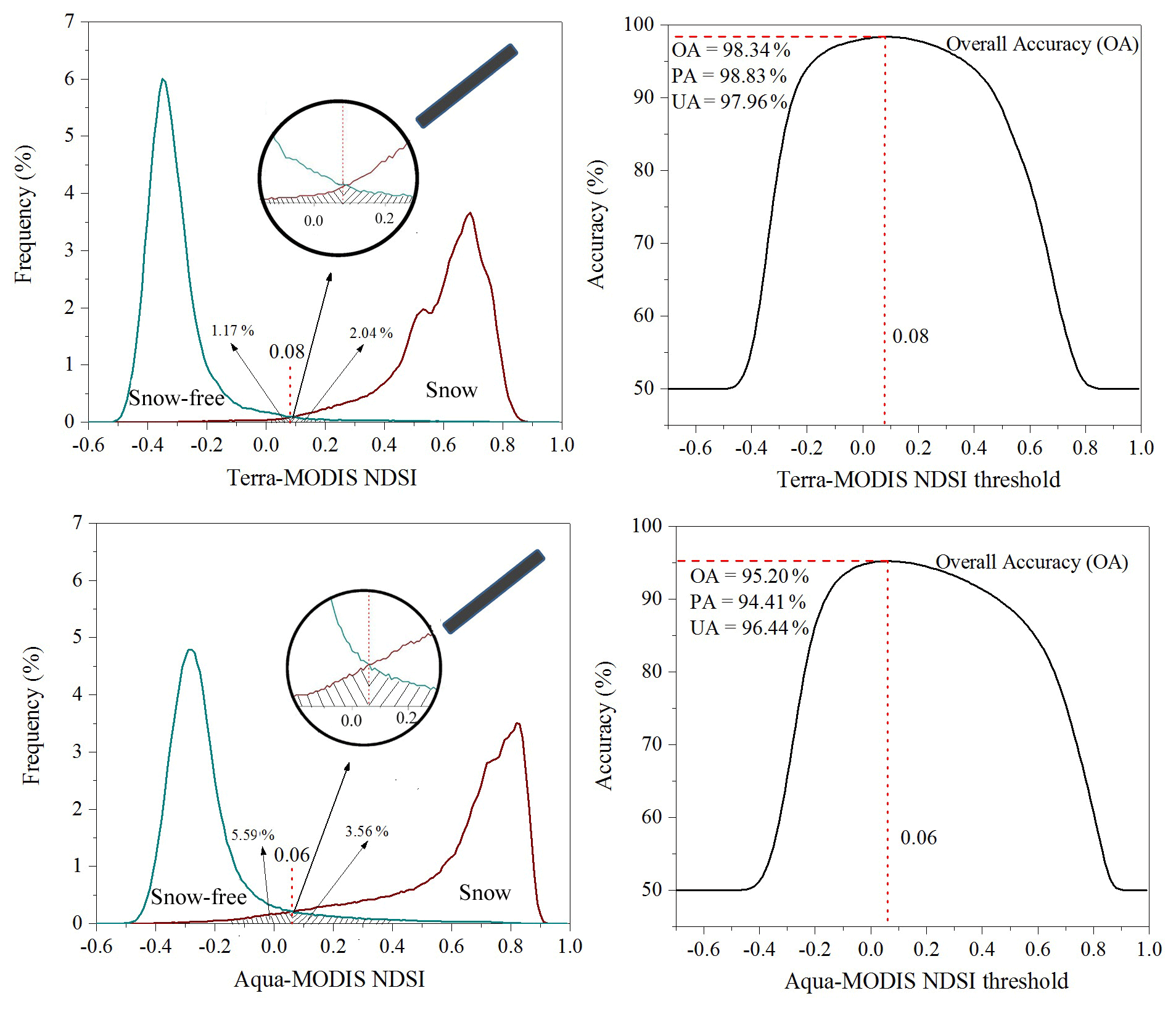
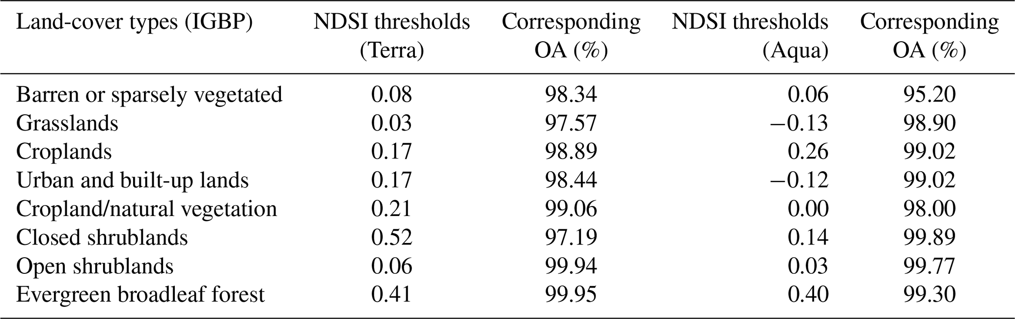
Following the same philosophy, the optimal NDSI thresholds for the other seven land-cover types, such as “grasslands”, “croplands”, “urban and built-up lands”, etc., are also obtained and listed in Table 1, together with their corresponding OAs. One can see that over these land-cover types the OAs are all larger than 95 %, which demonstrates the effectiveness of the new thresholds.

Table 1 Optimal NDSI thresholds over eight non-forest land-cover types.

However, as we expected, only using the NDSI criterion seems not accurate enough to discriminate snow cover over those forest land-cover types, except the “evergreen broadleaf forest” (due to its sparse distributions in China). For example, Fig. 3 gives the Terra-MODIS NDSI frequency distribution and the fluctuation of OAs over the “evergreen needleleaf forest”. Obviously, here the commission error (CE; see Sect. 5 for details) is very large (>35 %), and the OAs drop severely (<76 %). Therefore, for the remaining seven forest land-cover types, we will adopt a new decision rule as elaborated next.

Figure 3 Optimal NDSI thresholds over the land-cover type of “evergreen needleleaf forest”.

3.1.3 Optimized NDVI-NDFSI decision rules for forests

The study by Wang et al. (2015) had showed, compared with NDSI, that their so-called Normalized Difference Forest Snow Index (NDFSI, namely, using band 2 to substitute band 4 in Eq. 1) may be better for snow discrimination in forest areas. Our preliminary investigation reinforces this, and the improvement is, in particular, evident when using NDFSI in conjunction with NDVI (Wang et al., 2020).

Following their studies, NDVI in our study is divided into seven segments, and the optimal NDFSI at each NDVI segment will be computed with the highest OA as the object (similar to the acquirements of optimal NDSI thresholds). For a given pixel, if computed NDFSI is greater than the threshold in its corresponding NDVI segment, it will be regarded as a snow pixel; otherwise, it will be a snow-free pixel. With “deciduous broadleaf forest” as an example, Fig. 4 shows the NDVI-NDFSI number-density scatterplot that is derived from Terra-MODIS training samples over this land cover, as well as computed optimal NDFSI thresholds at every NDVI segment. Here the OA of the new NDVI-NDFSI decision rule is 99.91 % versus 88.77 % of the optimal NDSI threshold.

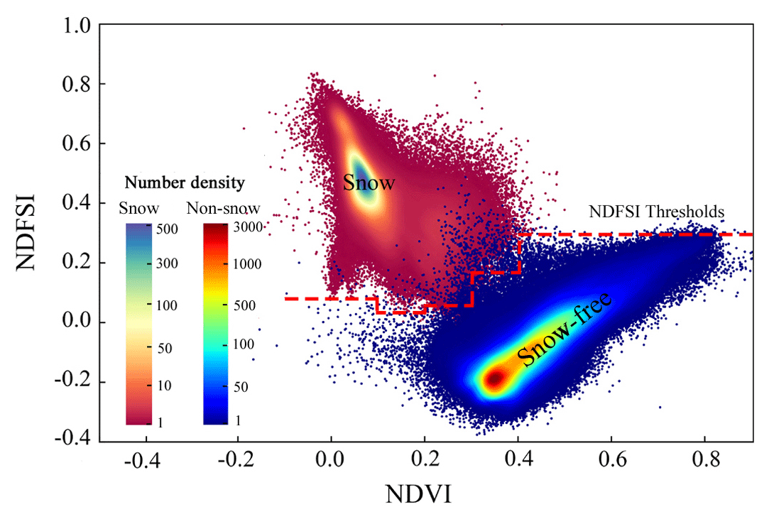
Figure 4 NDVI-NDFSI number-density scatterplot over “deciduous broadleaf forest” from Terra-MODIS training samples (colors represent the number density within a 0.01×0.01 bin).

Using this approach, optimized NDVI-NDFSI decision rules for the six left forest land-cover types are all determined. Tables 2 and 3 give the detailed NDVI-depending NDFSI thresholds for Terra-MODIS and Aqua-MODIS, respectively. Besides these thresholds, the tables also give the OAs of the optimized NDVI-NDFSI decision rules in the second last column and the OAs of the optimal NDSI thresholds in the last column. We can see that, compared with optimal NDSI thresholds, optimized NDVI-NDFSI decision rules increase OAs greatly. Using the optimal NDSI thresholds, most OAs are ≤90 %, whereas when using the optimized NDVI-NDFSI decision rules, most OAs are ≥96 %, in line with the accuracies of non-forest land-cover types in Table 1.

Table 2 Optimized Terra-MODIS NDVI-NDFSI decision rules for forest land-cover types (ENF: evergreen needleleaf forests; DNF: deciduous needleleaf forests; DBF: deciduous broadleaf forests; PWS: permanent wetland savannas).

^a refers to the OA of optimized NDVI-NDFSI decision rules. ^b refers to the OA of optimal NDSI thresholds.

Table 3 Optimized Aqua-MODIS NDVI-NDFSI decision rules for forest land-cover types.

3.1.4 Postprocessing based on surface temperature and DEM

Ice clouds have similar optical properties to snows. From time to time, pixels contaminated by broken ice clouds are mistaken for snow pixels, which will lead to some false snow existing even in the tropics. Like standard MODIS products (Riggs et al., 2006), we also use postprocessing based on surface temperature and DEM to reverse these snow pixels into snow-free pixels, but here ERA5 reanalysis LST (Munoz, 2019) is used rather than the brightness temperature from band 31.

According to our previous investigation (Hao et al., 2021), for lowlands of DEM <1300 m, snow at the surface basically impossibly exists when its temperature is ≥275 K (2 ^∘C), but for highlands of DEM ≥1300 m, a higher temperature threshold, 281 K (8 ^∘C), seems more appropriate due to the possible existence of warm snow on highlands (Riggs et al., 2016). Thereby, if snow is detected in a pixel when its height <1300 m and LST ≥275 K, this snow decision would be reversed to snow free. If snow is detected in a pixel when its height ≥1300 m and LST ≥281 K, this snow decision would also be reversed to snow free. Such a postprocessing is very effective to alleviate the problem of false snow detections, which are often seen in summers or over south China (when and where snow is impossible).

3.2 Cloud-gap-removing algorithm

Figure 5 describes the flow of the new cloud-gap-removing algorithm we developed in this study. It can be divided into three steps. The first step is preliminarily excluding some cloud gaps by the synergy of Terra-MODIS and Aqua-MODIS; the second step is further filling gaps according to the implication of the nearby clear-sky pixels using the hidden Markov random field (HMRF) technique; and in step three all left gaps will be filled using the auxiliary passive microwave product.

Figure 5 Flowchart of the new cloud-gap-removing algorithm.

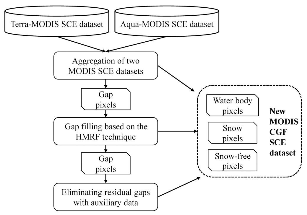
3.2.1 Aggregation of Terra-MODIS and Aqua-MODIS

There may be different weather conditions when Terra and Aqua pass in a day, and their synergy can reduce cloud gaps approximately by 10 %–30 % over China (Huang et al., 2016). Thus, in this study, we will first aggregate the Terra-MODIS SCE and Aqua-MODIS SCE under clear skies to preliminarily exclude some cloud gaps. The aggregating rule is as follows. In a day, if Terra-MODIS indicates a clear sky, its SCE information will be adopted; Otherwise, if Aqua-MODIS indicates a clear sky, Aqua-MODIS SCE information will be adopted. If both indicate a cloudy sky, the cloud gap is kept in that day.

3.2.2 Gap-filling based on the HMRF technique

For the aggregated SCE data, we will adopt the method based on the spatiotemporal hidden Markov random field (HMRF) proposed by Huang et al. (2018) to further fill gaps. The core of this method is computing the total spatiotemporal “energy” (probability) of belonging to snow pixels or snow-free pixels at one specific gap, using

$$\begin{array}{}\text{(2)}& {\displaystyle }U\left(\text{Snow}\right)=U_{\mathrm{st}}\left(\text{Snow}\left|N_{\mathrm{s}},N_{\mathrm{t}}\right.\right),\text{(3)}& {\displaystyle }U\left(\text{Snow-free}\right)=U_{\mathrm{st}}\left(\text{Snow-free}\left|N_{\mathrm{s}},N_{\mathrm{t}}\right.\right),\end{array}$$

where U_st is the spatiotemporal neighborhood energy function. N_s and N_t denote the spatial neighborhood and temporal neighborhood cantered with the gap, respectively.

Figure 6 illustrates our gap-filling process based on the HMRF technique. For a given gap, we will first calculate the U(Snow) and U(Snow-free) based on the 3 (row) ×3 (column) × 3 (day) spatiotemporal neighborhood. If the U(Snow) is greater than the U(Snow-free), the gap will be classified as snow pixels; otherwise, it will be classified as snow-free pixels. If there are not sufficient valid pixels for calculating the U(Snow) or U(Snow-free), we will extend the spatiotemporal neighborhood to 3 (row) × 3 (column) × 5 (day). If there are still not sufficient valid pixels, the spatiotemporal neighborhood will expand into 5 (row) × 5 (column) × 5 (day). If the above tries all fail, the gap will be kept still.

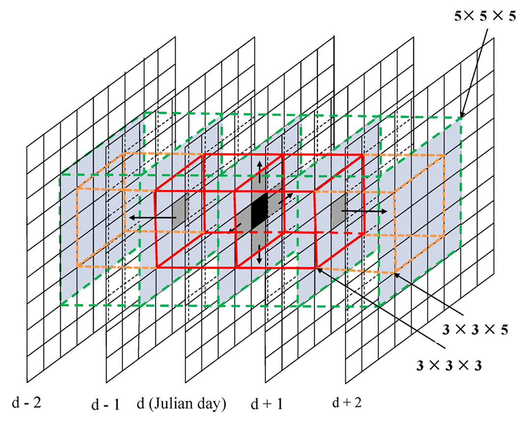
Figure 6 Diagram of the HMRF gap-filling process used in this study (dark grey represents high weight, and light grey represents low weight).

The gap-filling technique based on the HMRF provides a rigorous analytical framework for integrating spatial and temporal contexts in an optimal manner, which is accurate and highly efficient for MODIS cloud-gap filling (Huang et al., 2018). Our investigation shows that this method can remove approximately 80 % of the gaps in the aggregated data.

3.2.3 Eliminating residual gaps with auxiliary data

Although most cloud gaps have been filled after the two above processes, there are still a few exceptions. In this phase, we will use the auxiliary passive microwave snow-depth product provided by Che et al. (2008) to eliminate all remaining gaps. If colocated snow depth is ≥2 cm, then the gap will be assigned a snow pixel; otherwise, it will be a snow-free pixel (Hao et al., 2019).

4 Product

Using the new snow discrimination algorithm developed for clear skies in Sect. 3.1, we produce a new Terra-MODIS SCE dataset and a new Aqua-MODIS SCE dataset over China with MOD09GA and MYD09GA products as the main inputs. There are four classes of pixels in the new datasets, namely, snow, snow free, water body, and gap (see Fig. 7). Because optical remote sensing is affected by clouds severely, there are often abundant gaps (up to 70 %) in such clear-sky products, which limit their application to a very great extent.

Figure 7 NIEER MODIS SCE product on 4 January 2020: (a) Terra-MODIS SCE dataset; (b) Aqua-MODIS SCE dataset; (c) CGF-MODIS SCE dataset.

Next, based on the two clear-sky datasets above, we produce a new CGF SCE dataset using the new cloud-gap-removing algorithm developed in Sect. 3.2. In the new dataset, all gaps have been removed, and only three classes (snow, snow free, and water body) are included (see Fig. 7). Comparing with the first two datasets, this dataset undoubtedly has a wider application prospect.

The new Terra-MODIS, Aqua-MODIS, and CGF-MODIS SCE datasets together constitute the NIEER MODIS SCE product (Hao et al., 2021). It has a 500 m spatial resolution and a daily temporal resolution, providing the snow-cover condition in the past two decades over China. An instance of snow coverage revealed by the product is presented in Fig. 7.

5 Validation

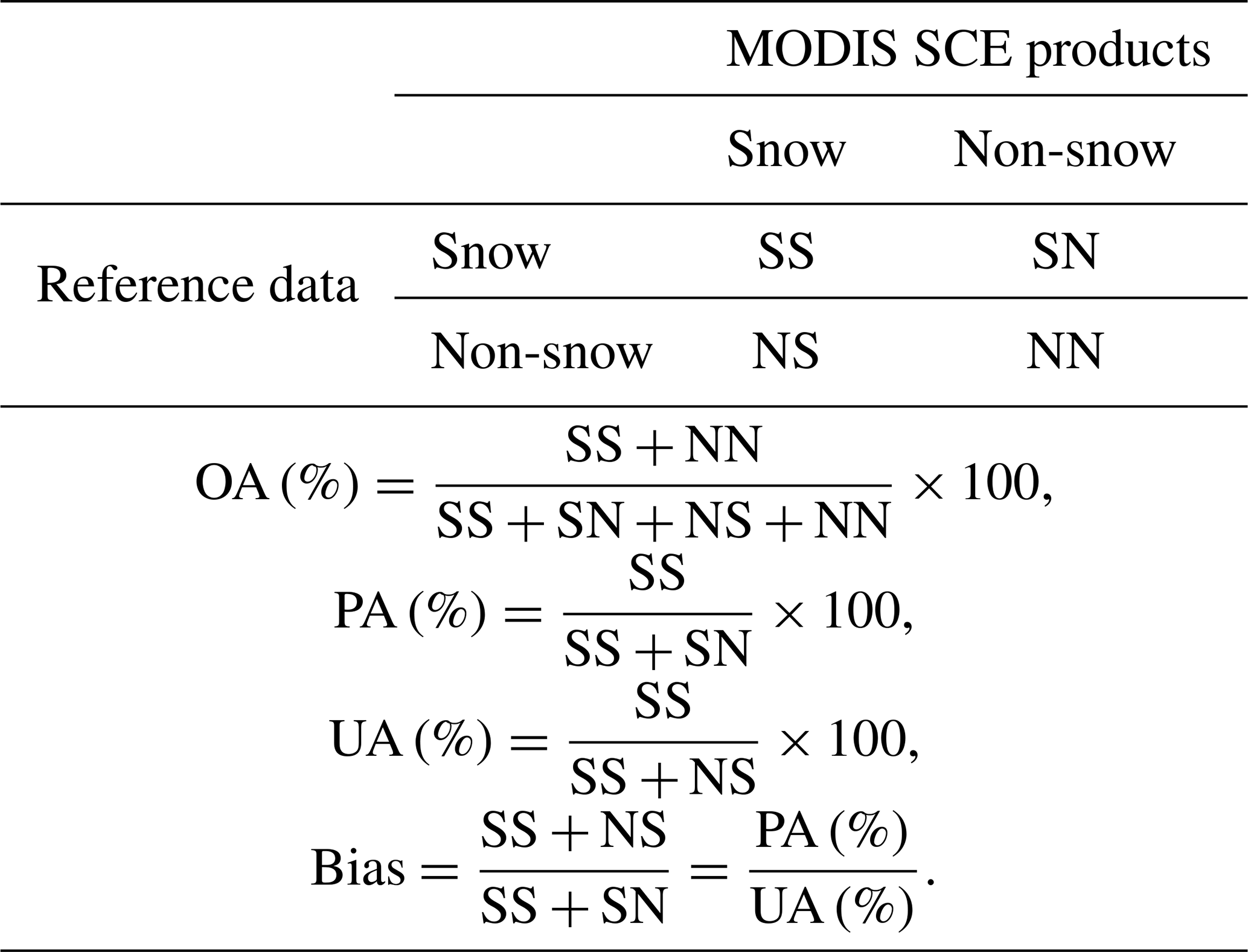
A confusion matrix similar to Table 4 is used to validate or assess all associated MODIS SCE data in this study. The overall accuracy (OA) represents the percentage that snow and snow-free pixels are correctly classified, the producer's accuracy (PA, corresponding to the omission error, $\text{OE}=\mathrm{1}-\text{PA}$) represents the percentage that real snow pixels are classified as such, and the user's accuracy (UA, corresponding to the commission error, $\text{CE}=\mathrm{1}-\text{UA}$) represents the percentage that pixels classified as snow are also snow in reality. Because the kappa coefficient has caused too much controversy recently (Pontius and Millones, 2011; Stehman and Foody, 2019), we no longer use it as an accuracy metric here. Meanwhile, to more directly show whether SCE is overestimated or underestimated and to what extent, a metric termed as “bias” is introduced. The bias, defined as the ratio of pixels classified as snow to real snow pixels (Hüsler et al., 2012; Wu et al., 2021), is a relative measure to detect overestimation (values >1) or underestimation of snow (values <1).

Table 4 Description of the confusion matrix used to validate or assess the associated SCE products (SS, SN, NS, and NN are the numbers in each case).

Note that nominally 20-year and 362-station snow-depth measurements will be used as reference data to validate our product, but in fact validations are conducted only during the snow seasons at one station when the snow-cover days are ≥20; otherwise, some accuracy metrics would become artificially high due to too many non-snow pixels in a mid-latitude region like China (Hao et al., 2008).

5.1 Overview of the new product's accuracies

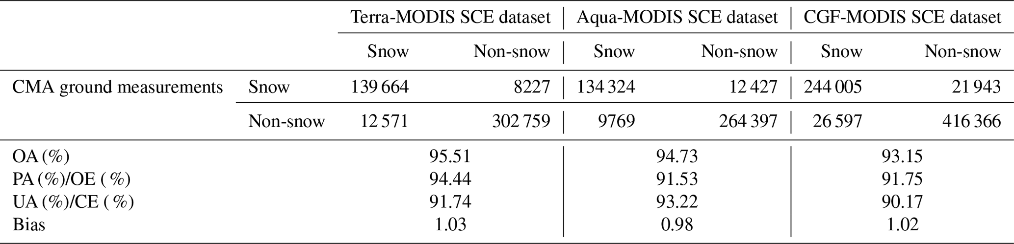
In Table 5, an overview is given of validation results for the new MODIS SCE product. We can see on a whole that the two new clear-sky datasets are very accurate. For the Terra-MODIS SCE dataset, the OA, OE, and CE are 95.51 %, 5.56 %, and 8.26 %, respectively; for the Aqua-MODIS SCE dataset, the OA, OE, and CE are 94.73 %, 8.47 %, and 6.78 %, respectively. The former has a lower omission error, while the latter has a lower commission error. From the bias point of view, the Terra-MODIS dataset slightly overestimates snow cover, and the Aqua-MODIS dataset slightly underestimates snow cover. But from the specific values (1.03 and 0.98), the overestimation and underestimation are marginal. Comparatively speaking, the Aqua-MODIS dataset is inferior to the Terra-MODIS dataset. This is not surprising considering the problem of the Aqua-MODIS band 6 and the fact that CMA snow-depth measurement is only conducted in the mornings.

Although the CGF-MODIS SCE dataset is slightly worse than the two clear-sky datasets, there is no significant difference no matter what accuracy metric is used. Here the OA, OE, and CE are 93.15 %, 8.25 %, and 9.83 %, respectively. Compared with the metrics shown above, the accuracy drops are basically within 1–2 percentage points. Moreover, the bias of 1.02 also demonstrates an inconspicuous overestimation. Therefore, our cloud-gap-removing processes are effective, and the accuracy may be sustained at a consistent level as the clear-sky datasets.

Table 5 Validation results of the new NIEER MODIS SCE product with reference to CMA ground measurements.

5.2 The stability in time

To assess the stability of the NIEER MODIS SCE product in time, the accuracy metrics in every snow season since 2000 are calculated separately. Figure 8 presents the interannual fluctuation of these accuracy metrics. From the figure, we can see that all three datasets have a similar fluctuation characteristic. They always perform a consistent high accuracy in one snow season, and a coincident low accuracy in another snow season. Such an accuracy fluctuation may be attributed to the different validation numbers available in different years caused by ground measurements.

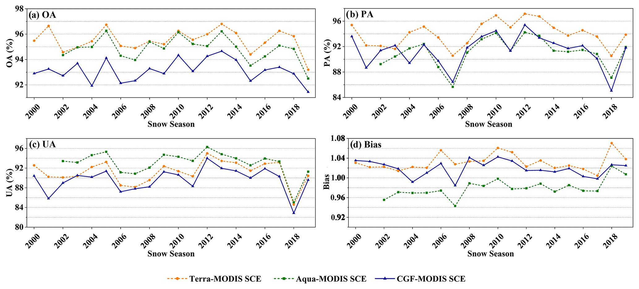
Figure 8 Annual accuracy metrics' fluctuation of the NIEER MODIS SCE product: (a) OA, (b) PA, (c) UA, and (d) Bias.

The highest accuracy happens in the snow season of 2012, where the OEs of the three datasets are 2.84 %, 5.76 %, and 4.60 %, and the CEs are 5.02 %, 3.72 %, and 6.01 %. Meanwhile, the worst accuracy happens in the snow season of 2018, where the OEs of the three datasets are 9.49 %, 12.91 %, and 14.95 %, and the CEs are 15.42 %, 14.96 %, and 17.15 %. But except this snow season, the OEs and CEs in other seasons are all less than 15 %. Relative to OE and CE (namely, PA and UA), OA fluctuations of the three datasets are smaller. The Terra-MODIS dataset fluctuates within 93 %–97 %, the Aqua-MODIS dataset fluctuates within 93 %–96 %, and the CGF-MODIS dataset fluctuates within 92 %–95 %.

In addition, from the bias point of view, the values ranging from 0.94 to 1.07 demonstrate that there are neither substantial overestimations nor substantial underestimations in all datasets and snow seasons. Therefore, on average the new product is stable in time and promising to better serve the climatic, hydrological, and other related studies in China (Huang et al., 2020).

5.3 The reliability in space

To clarify the new product's reliability in space, we calculate accuracies at each CMA station. With the Terra-MODIS SCE dataset as an example, Fig. 9 presents the detailed accuracies. From the figure, we find, in spite of a very high accuracy seen at most stations, the errors may be relatively larger in the southwest of Northeast China and the northeastern edges of Qinghai–Tibet Plateau. This can be attributed to their patchy snow-cover features and rugged terrains (Xiao et al., 2020), where Loess Plateau and Qinghai–Tibet Plateau rapidly transit toward Sichuan Basin and Northeast Plain, respectively. The Aqua-MODIS SCE dataset performs a very similar accuracy pattern like Fig. 9 but slightly worse.

Figure 9 Accuracies of the Terra-MODIS SCE dataset at each CMA station: (a) OA, (b) PA, (c) UA, and (d) Bias.

Figure 10 further details the accuracies of the CGF-MODIS SCE dataset at all stations. From the figure, we see that in North Xinjiang and the north of Northeast China, where the snowpack is stable, the accuracy is high, whereas in the northeast of Inner Mongolia Autonomous Region, the northwest of North China, and Qinghai–Tibet Plateau, where snow may melt rapidly even in winter, the accuracy is relatively lower. Besides the propagated errors from the two original clear-sky SCE datasets, it is supposed that an unstable snowpack in warmer areas would result in another large uncertainty.

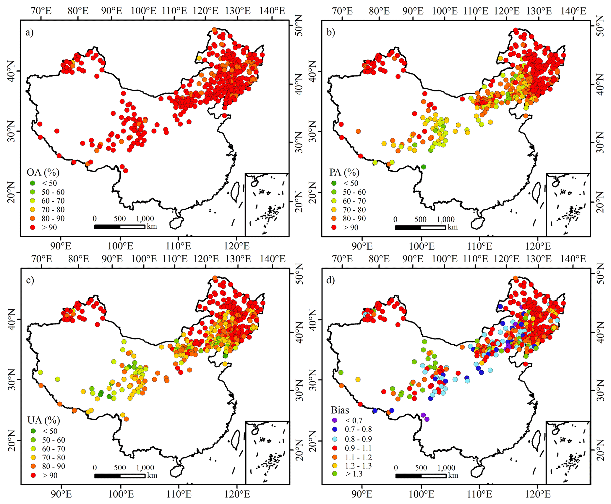
Figure 10 Accuracies of the CGF-MODIS SCE dataset at each CMA station: (a) OA, (b) PA, (c) UA, and (d) Bias.

6 Discussion

6.1 Comparisons with standard MODIS products

Using the same ground reference data, we also evaluate the standard SCE data derived from the newest C6.1 MOD10A1, MYD10A1, MOD10A1F, and MYD10A1F products (see Table 6). Comparing the accuracy metrics listed here and those in Table 5, we can see that these products' accuracies are significantly lower than our product's accuracy. If ground measurements are seen as true values, the MOD10A1 product's OE and CE values are 7.22 % and 12.97 %, respectively, versus 5.56 % and 8.26 % of our Terra-MODIS dataset; the MYD10A1 product's OE and CE values are 13.78 % and 23.78 %, respectively, versus 8.47 % and 6.78 % of our Aqua-MODIS dataset. Our improvement is particularly significant for Aqua-MODIS SCE, where the CE is improved by over 17 percentage points. Besides, from the bias point of view, there are appreciable overestimations to snow cover in standard MOD10A1 and MYD10A1 products.

Note that here factual improvement may be much more obvious than shown by the accuracy metric of OA, because there are a large number of non-snow pixels (far beyond snow pixels) in a mid-latitude region like China, which would pull it up dramatically. Although the new product's improvement in OA is within 1 % relative to MOD10A1 products, in fact the OE has decreased by 37 %, and the CE has decreased by 22 %.

Table 6 Accuracies of SCE products derived from MOD10A1, MYD10A1, MOD10A1F, and MYD10A1F using the same ground measurements.

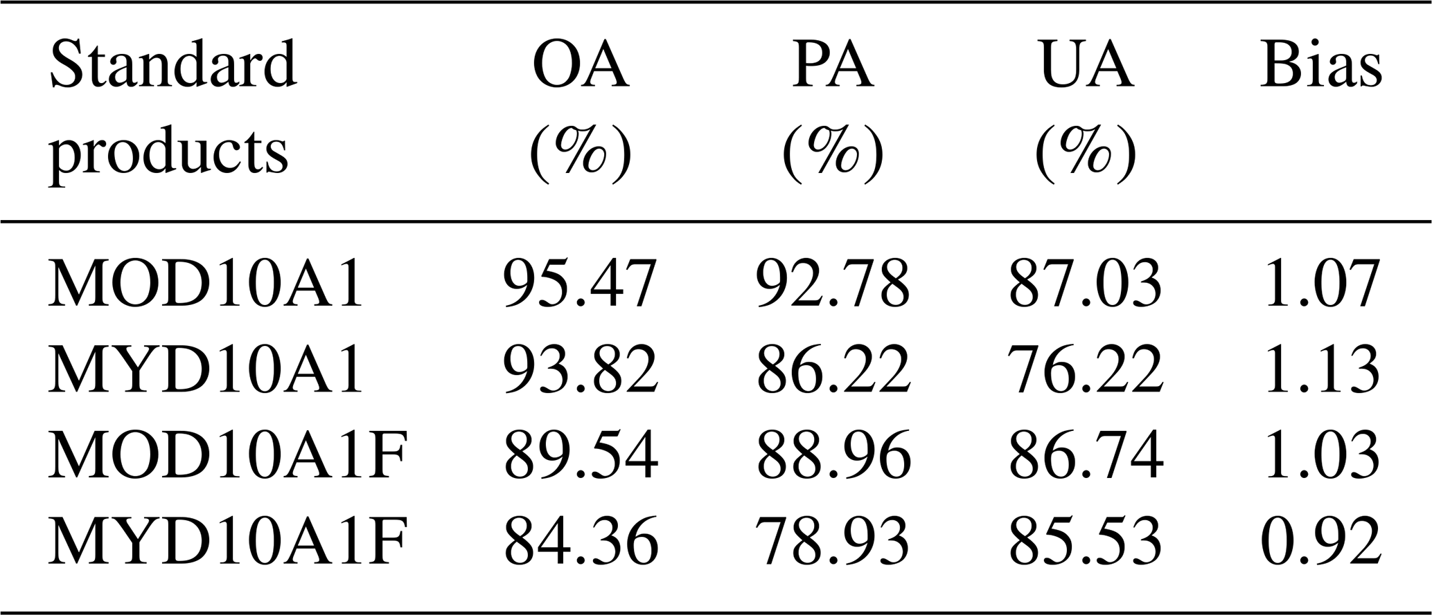
Due to possible wider application, the CGF product comparison is emphasized here. Relative to the better standard product (MOD10A1F), our product's OA increases by nearly 4 percentage points, the OE drops from 11.04 % to 8.43 %, and the CE drops from 13.26 % to 9.83 %; relative to the worse standard product (MYD10A1F), the OA even increases by nearly 9 percentage points, the OE drops from 21.07 % to 8.25 %, and the CE drops from 14.47 % to 9.83 %. It is clear for the standard CGF products that all of the OEs and CEs are larger than 10 %, while for our product the OE and CE are both within 10 %. Meanwhile, the two standard CGF products' biases are also further away from 1. Therefore, our improvement to CGF SCE is obvious, too. Besides, comparing the two standard clear-sky products with the two standard CGF products, we find their cloud-gap-removing strategy indeed lowers the accuracies dramatically.

6.2 Improvement in forest areas

To figure out the improvement in forest areas, the validations and comparisons at four forest CMA stations are isolated and listed in Table 7. From the table, one can see the OA increases by 3–10 percentage points, the OE drops by 1–8 percentage points, and the CE drops by 4–21 percentage points. As well, more significant improvements are seen for the Aqua-MODIS and the CGF SCE datasets. For example, the CE of the new Aqua-MODIS SCE dataset has already dropped to 9.62 %, comparing with 30.13 % of MYD10A1 product; the OA of the new CGF-MODIS dataset increases to 91.23 %, compared with 81.79 % of MOD10A1F product. Thus, the improvement of the new product in forest areas is also considerably significant, even more significant than in non-forest areas.

Table 7 Validation and comparison at four forest CMA stations.

Two more intuitional examples are shown in Fig. 11. One is a typical forest area in Northeast China on 1 January 2018; another comes from southeastern forest regions of Qinghai–Tibet Plateau on 1 February 2018. It is clear that the new CGF-MODIS SCE dataset agrees much better with the higher-resolution snow maps than the standard CGF product does. The standard MOD10A1F perceivably overestimates snow coverage in these forest areas.

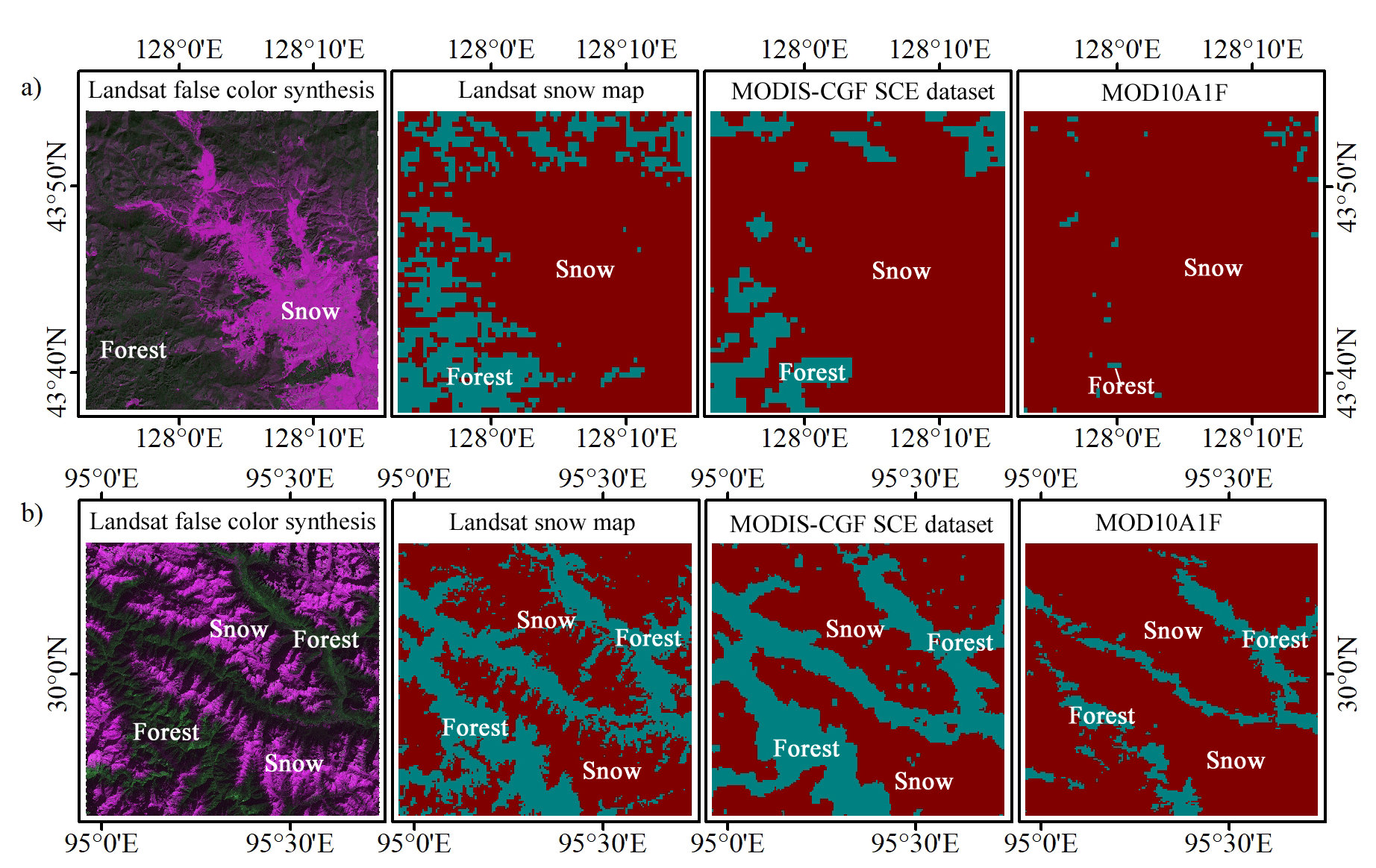
Figure 11 Intuitional improvements of CGF SCE in two representative forest areas: (a) an example in a Northeast China forest region; (b) an example in the Qinghai–Tibet Plateau forest region.

Of course, the new product is far from perfect. In particular, the product's performance is limited severely by the cloud mask provided by standard MOD09GA/MYD09GA products, which is virtually caused by the cloud/snow confusion problem. On the one hand, some broken ice clouds are susceptible to being mistaken for snow pixels because of their similar optical properties, which will result in some artificial snow pixels in South China (although it has been mitigated largely compared with the standard MODIS snow products). On the other hand, snow pixels are also possibly mistaken for clouds, which will result in some omitted snow covers. During our validations or comparisons, we found this phenomenon is somewhat common in the edges of snow-cover areas and the forest areas of Northeast China.

7 Summary and outlook

In this study, we produce a new MODIS SCE product over China, which is committed to addressing currently known problems of the standard snow products. Therefore, the optimal NDSI thresholds varying with land-cover types are extracted, and the NDVI-NDFSI decision rules proposed by Wang et al. (2015) specific for snow discrimination in forest areas are optimized by a number of training samples indicated by the higher-resolution snow maps from Landsat-8 OLI images. Meanwhile, to obtain a daily continuous cloud-free SCE dataset, the clear-sky snow SCE data from Terra-MODIS and Aqua-MODIS are aggregated first; an HMRF gap-filling technique, which can simultaneously assimilate temporally and spatially neighboring information, is imported second; finally, the residual gaps are all filled according to the implication given by an auxiliary passive microwave snow-depth dataset.

The new product is named the NIEER MODIS SCE product, which contains three individual datasets – the Terra-MODIS SCE dataset, the Aqua-MODIS SCE dataset, and the MODIS CGF SCE dataset. The first two provide the SCE knowledge under clear skies directly derived from the MODIS surface reflectance products, while the last provides daily and totally continuous SCE knowledge.

The comprehensive validations against 362 CMA stations across China have revealed that our product is not only very accurate but also considerably stable in time and reliable in space. On a whole, there are no significant overestimations nor any significant underestimations in all datasets, and the cloud-gap-removing processes do not lower the SCE accuracy severely. Compared with SCE indicated by the standard MODIS snow products, our product's accuracies are obviously higher, especially for the Aqua-MODIS and CGF SCE datasets. Relative to the MYD10A1 product, the CE drops 17 percentage points, from 23.78 % to 6.78 %. Relative to the better MOD10A1F CGF product, the OA increases by nearly 4 percentage points, from 89.54 % to 93.15 %. Meanwhile, as we expected, the improvement in forest areas is also evident. If validations at forest stations are isolated, OA increases by 3–15 percentage points. Therefore, the new product has provided more reliable knowledge on snow coverage over China and thereby will be a better choice for climatic, hydrological, and other related studies there.

The problem of cloud/snow confusion may contribute to the largest uncertainty in the new product. There are many cases when snow pixels are mistaken for cloudy pixels or the opposite case due to the inaccurate cloud mask provided by MOD09GA/MYD09GA products. In the future, we will consider further improving our product from this aspect.