Testing a maximum evaporation theory over saturated land: implications for potential evaporation estimation

State-of-the-art evaporation models usually assume net radiation (R_n) and surface temperature (T_s; or near-surface air temperature) to be independent forcings on evaporation. However, R_n depends directly on T_s via outgoing longwave radiation, and this creates a physical coupling between R_n and T_s that extends to evaporation. In this study, we test a maximum evaporation theory originally developed for the global ocean over saturated land surfaces, which explicitly acknowledges the interactions between radiation, T_s, and evaporation. Similar to the ocean surface, we find that a maximum evaporation (LE_max) emerges over saturated land that represents a generic trade-off between a lower R_n and a higher evaporation fraction as T_s increases. Compared with flux site observations at the daily scale, we show that LE_max corresponds well to observed evaporation under non-water-limited conditions and that the T_s value at which LE_max occurs also corresponds with the observed T_s. Our results suggest that saturated land surfaces behave essentially the same as ocean surfaces at timescales longer than a day and further imply that the maximum evaporation concept is a natural attribute of saturated land surfaces, which can be the basis of a new approach to estimating evaporation.

1 Introduction

Potential evaporation (E_P), defined as the rate of evaporation (E) that would occur under non-water-stressed conditions, determines the upper boundary of E over a specific land surface for a given meteorological forcing. Although E_P is more of a hypothetical variable and is generally very difficult to observe, it is often the starting point for partitioning rainfall between E, runoff, and soil moisture changes in hydrological, agricultural, ecological, and other related studies (Maes et al., 2019; Milly and Dunne, 2016; Scheff and Frierson, 2014; Schellekens et al., 2017; Sheffield et al., 2012; Vicente-Serrano et al., 2013; Wang and Dickinson, 2012). Over the years, numerous mathematical models have been proposed with varying structures and complexities to quantify E_P (e.g., Allen et al., 1998; Priestley and Taylor, 1972; Penman, 1948; Shuttleworth, 1993; Thornthwaite, 1948). Among them, the Penman–Monteith type models (e.g., either the Open Water Penman model; Shuttleworth, 1993; or the Food and Agriculture Organization Penman–Monteith model; Allen et al., 1998) are most widely used, given their explicit consideration of the radiative and aerodynamic components of E, and are hence generally considered as a physical-based and accurate approximation of the real E processes.

Nevertheless, recent empirical evidence shows that the Penman–Monteith type models perform unsatisfactorily in estimating E_P compared with eddy covariance observations (i.e., the observed E under non-water-stressed conditions; Maes et al., 2019). Instead, the energy balance-based approaches work better in reproducing E_P in both observations (Maes et al., 2019) and climate model simulations (Milly and Dunne, 2016). From an energy balance point of view, the magnitude of E (or in its energy form – latent heat flux or LE) is determined by the energy balance equation:

$$\begin{array}{}\text{(1)}& LE=\left(R_{\mathrm{n}}-G\right){\displaystyle \frac{\mathrm{1}}{\mathrm{1}+\mathit{\beta }}},\end{array}$$

with R_n the net radiation (W m⁻²) and G the ground heat flux (W m⁻²), which is often negligibly small over land for timescales longer than a day. In Eq. (1), β is the Bowen ratio and represents the ratio of sensible heat flux (H) over LE (Bowen, 1926). As a result, LE is determined by the available energy at an evaporating surface (i.e., R_n−G) and the ability of that evaporating surface to convert the available energy into LE, which is represented by the $\mathrm{1}/(\mathrm{1}+\mathit{\beta })$ term and is often known as the evaporative fraction. With no restriction on water supply, β is known to be a decreasing function of temperature at an evaporating surface (T_s; Aminzadeh et al., 2016; Andreas et al., 2013; Guo et al., 2015; Philip, 1987; Priestley and Taylor, 1972; Slatyer and McIlroy, 1961; Yang and Roderick, 2019). This implies that when water is not limiting, both T_s and the available energy determine the rate of E. Hence, with fixed available energy, a higher T_s corresponds to a lower β (or a higher evaporative fraction) and therefore a larger LE. This line of reasoning has directly led to the development of energy balance-based evaporation models, including the classic equilibrium evaporation approach (Slatyer and McIlroy, 1961) and the Priestley–Taylor evaporation model (Priestley and Taylor, 1972). Compared with Penman–Monteith type models, the energy balance-based approach simplifies the representation of the aerodynamic component of E and usually takes the aerodynamic component of E as a fixed fraction of its radiative counterpart (e.g., 0.26 in the Priestley–Taylor model).

However, a key issue in the above energy balance-based approach is that it takes R_n to be an independent forcing of E. A similar idea was also adopted in Penman–Monteith type models (Penman, 1948; Monteith, 1965). Nevertheless, it is clear that R_n cannot be physically independent of either E or T_s. On one hand, a higher T_s corresponds to higher outgoing longwave radiation and therefore a lower R_n. On the other hand, a higher E is associated with larger evaporative cooling, which lowers T_s and ultimately feed backs to R_n. This latter process confirms that T_s is not independent of E. Consequently, the intrinsic interdependence between R_n, E, and T_s has long been ignored in the state-of-the-art evaporation models that require R_n as model input (Yang and Roderick, 2019).

To deal with the above issue, a recent study by Yang and Roderick (2019) explicitly considered the interdependence between radiation, T_s, and evaporation and tested the new approach over global ocean surfaces. They found that with the increase of T_s, R_n decreases while evaporative fraction increases (since β decreases as T_s increases), in agreement with a number of previous studies (Aminzadeh et al., 2016; Andreas et al., 2013; Guo et al., 2015; Philip, 1987; Priestley and Taylor, 1972; Slatyer and McIlroy, 1961). This generic and explicit trade-off between a lower R_n and a higher evaporative fraction with the increase of T_s directly yields a maximum evaporation along the T_s gradient according to Eq. (1) (Yang and Roderick, 2019; also see Sect. 2.2). This maximum evaporation emerges naturally from the R_n–T_s–E interactions and does not require a priori knowledge of T_s thereby alleviating the need for the assumption that R_n and T_s are independent of E in traditional evaporation models. As a result, the maximum evaporation theory does not consider R_n to be an independent forcing of E. Instead, it only requires the incoming and reflected solar radiation and the assumption that β decreases with the increase of T_s (see Sect. 2.2). Compared with observations of ocean surface evaporation and temperature, Yang and Roderick (2019) demonstrated the validity of the maximum evaporation theory over global ocean surfaces. Here, we test this new maximum evaporation theory over land by asking and answering two questions: (i) does the theory recover the observed E and (ii) does it recover the observed T_s? By recovering, we mean that the maximum E as per theory corresponds to the observed E and that the T_s at which the maximum E occurs corresponds to the observed T_s under non-water-stressed conditions. Testing the maximum evaporation theory over land is important, as vegetation transpiration generally dominates the total evaporative flux over land (Jasechko et al., 2013; Lian et al., 2018), which is essentially different from ocean surfaces where the evaporative flux only consists of evaporation from open water surfaces. In addition, land surfaces usually have a larger surface roughness than ocean surfaces, which may result in different energy partitioning (into sensible heat and latent heat) between the ocean and the land. Therefore, it is crucial to test the maximum evaporation theory over land to determine whether saturated land behaves like the ocean surface and whether the maximum evaporation theory can be the basis of a new approach to estimating E_P over land.

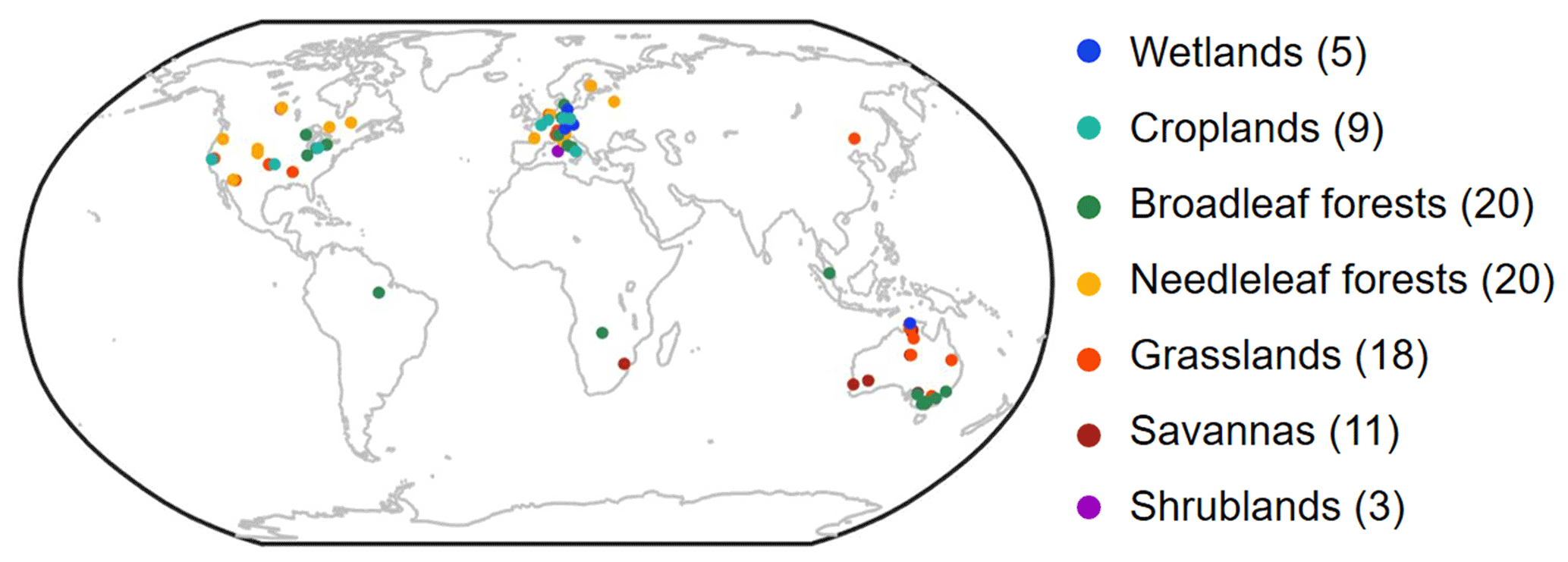
Figure 1 Location of the 86 flux sites used in this study. Numbers in the brackets indicate the number of sites for each biome type.

2 Materials and methods

2.1 Flux site observations

Observations of actual daily evaporation (or latent heat flux), sensible heat flux, and ground heat flux along with relevant meteorological variables, radiative fluxes and soil moisture were originally obtained from 212 flux sites collected in the FLUXNET2015 database (http://fluxnet.fluxdata.org/data/fluxnet2015-dataset/, last access: 2 November 2020). Only days with the data quality metric for LE and H higher than 0.9 (on a scale of 0–1) were used. The daily scale variables were obtained based on 15 min/30 min observations using the standard approach (Pastorello et al., 2020). The residual approach (i.e., assuming the observed H is correct and considering LE as the residual of the energy balance equation) was used to recalculate the fluxes based on a forced energy balance closure at each flux site (Ershadi et al., 2014). We also used the Bowen ratio approach (Twine et al., 2000) to force the flux-site energy balance closure and this resulted in similar model performance (Fig. S1 in the Supplement). The surface temperature for each site-day combination was calculated based on the observed longwave radiation following:

$$\begin{array}{}\text{(2)}& T_{\mathrm{s}}=\sqrt[\mathrm{4}]{{\displaystyle \frac{R_{\mathrm{lo}}-(\mathrm{1}-\mathit{\epsilon })R_{\mathrm{li}}}{\mathit{\epsilon }\mathit{\sigma }}}},\end{array}$$

where R_lo and R_li are, respectively, the outgoing and incoming longwave radiation, σ is the Stefan–Boltzmann constant ($\mathrm{5.67}\times {\mathrm{10}}^{-\mathrm{8}}$ W m⁻² K⁻⁴), and ε is the surface emissivity, which is acquired from the MODIS (Moderate Resolution Imaging Spectroradiometer) emissivity product (i.e., MOD11A1 Version 6; https://lpdaac.usgs.gov/products/mod11a1v006, last access: 2 January 2021). The MOD11A1 surface emissivity has a daily temporal resolution and a 1 km spatial resolution. To obtain the emissivity for each eddy covariance (EC) flux site, we center on the pixel where the site is located and take the mean value of the 81 neighboring pixels (9×9 pixels) as the emissivity value of the site. For conditions when the MOD11A1 emissivity are not available, we deleted these site-days.

To select a subset of observations at each flux site in which the actual evaporation is not limited by water availability, the energy balance criterion and the soil moisture criterion used by Maes et al. (2019) were adopted. Specifically, at each flux site, the evaporative fraction (EF; i.e., $\mathrm{EF}=LE/(LE+H))$ was first calculated and the unstressed measurements consisted of all days with EF exceeding the 95th percentile EF threshold at each site. Following that, we removed days with soil moisture (averaged over all measured depths) lower than 50 % of the maximum soil moisture (taken to be soil moisture at the 98th percentile) at each site. In addition, any remaining site-days with daily EF values lower than 0.6 were also removed. Finally, we removed days having a negative H value (accounting for ∼5 % of the total daily data) to avoid dealing with strongly advective conditions when accurate measurements are not guaranteed (Paw U et al., 2000; Wilson et al., 2002). As a result, a total of 1128 non-water-stressed site-days from 86 sites passed the above criteria and were used in this study (Fig. 1 and Table S1 in the Supplement).

2.2 Maximum evaporation model

2.2.1 Overview of the maximum evaporation model

The maximum evaporation model calculates evaporation from a wet surface based essentially on the surface energy balance (Eq. 1), with R_n and β both explicitly represented as functions of T_s (Yang and Roderick, 2019):

$$\begin{array}{}\text{(3)}& LE={\displaystyle \frac{\mathrm{1}}{\mathrm{1}+\mathit{\beta }\left(T_{\mathrm{s}}\right)}}\left[R_{\mathrm{n}}\left(T_{\mathrm{s}}\right)-G\right].\end{array}$$

In the above equation, the first term on the right-hand side (i.e., $\mathrm{1}/[\mathrm{1}+\mathit{\beta }(T_{\mathrm{s}}\left)\right]$) is the evaporative fraction, which is the ratio of the latent heat flux over the total available energy. Over wet surfaces, since the Bowen ratio decreases with T_s (Aminzadeh et al., 2016; Andreas et al., 2013; Guo et al., 2015; Philip, 1987; Priestley and Taylor, 1972; Slatyer and McIlroy, 1961; Yang and Roderick, 2019), evaporative fraction increases with T_s. On the other hand, the second term on the right-hand side of Eq. (3) is the total available energy, which decreases with the increase of T_s as a higher T_s directly leads to a higher outgoing longwave radiation and hence a lower R_n (Yang and Roderick, 2019). As a result, the trade-off between a higher evaporative fraction and a lower R_n with the increase of T_s would naturally lead to a maximum LE along the T_s gradient according to Eq. (3). A previous study by Yang and Roderick (2019) demonstrated that this naturally emergent maximum LE corresponds well to the actual LE over global ocean surfaces and the T_s at which the maximum LE occurs also corresponds to the observed sea surface temperature. Here we will test whether this maximum evaporation approach is also valid over land under non-water-stressed conditions.

2.2.2 Parameterization of R_n and β as a function of T_s

To explicitly acknowledge the dependence of R_n on T_s, R_n(T_s) is expressed as

$$\begin{array}{}\text{(4)}& R_{\mathrm{n}}\left(T_{\mathrm{s}}\right)=R_{\mathrm{sn}}+\mathit{\epsilon }\mathit{\sigma }{\left(T_{\mathrm{s}}-\mathrm{\Delta }T\right)}^{\mathrm{4}}-\mathit{\epsilon }\mathit{\sigma }{T}_{\mathrm{s}}^{\mathrm{4}},\end{array}$$

where R_sn is the net shortwave radiation (W m⁻²) and is taken to be unchanged with T_s. ΔT is the temperature difference between T_s and the effective radiating temperature of the atmosphere (T_rad; assuming blackbody radiation, $T_{\mathrm{rad}}=\sqrt[\mathrm{4}]{R_{\mathrm{li}}/\mathit{\sigma }})$, and is parameterized as a function of atmospheric transmissivity and geographic latitude (Yang and Roderick, 2019):

$$\begin{array}{}\text{(5)}& \mathrm{\Delta }T=n_{\mathrm{1}}\exp \left(n_{\mathrm{2}}\mathit{\tau }\right)+n_{\mathrm{3}}\left|\mathrm{lat}\right|,\end{array}$$

where τ is the atmospheric transmissivity for shortwave radiation (dimensionless) and is calculated as the ratio of incoming shortwave radiation at the Earth's surface to that at the top of the atmosphere. The parameter “lat” is the geographic latitude (in decimal degrees), which is considered here to account for a longer pathway of shortwave radiation going through the atmosphere in higher latitudes compared to lower latitudes. n₁, n₂, and n₃ are the fitting coefficients. Using extensive data over the global ocean (n=202 794), Yang and Roderick (2019) determined the values of these coefficients to be n₁=2.52, n₂=2.38, and n₃=0.035, respectively. Here, we directly adopt these same coefficient values over land for two reasons: (i) the key processes governing the interactions between incoming and outgoing longwave radiation are essentially the same for ocean and land (mainly greenhouse gases that affect the vertical temperature structure of the atmosphere, and water vapor and aerosols that affect the formation of clouds), and (ii) there were many more samples available for parameterizing Eq. (5) over the ocean than that over land. Validation against observations from all 1128 non-water-limited site-days demonstrates an overall good performance of Eq. (5) in estimating ΔT over land under saturated conditions (Fig. S2).

The Bowen ratio (β) is expressed as a function of T_s:

$$\begin{array}{}\text{(6)}& \mathit{\beta }\left(T_{\mathrm{s}}\right)=m{\displaystyle \frac{\mathit{\gamma }\left(T_{\mathrm{s}}\right)}{\mathrm{\Delta }\left(T_{\mathrm{s}}\right)}},\end{array}$$

where m is a fitting coefficient. γ is the psychrometric constant (kPa K⁻¹), and Δ is the slope of the saturation vapor pressure curve (kPa K⁻¹), both of which are functions of T_s:

$$\begin{array}{}\text{(7)}& {\displaystyle }& {\displaystyle }\mathit{\gamma }\left(T_{\mathrm{s}}\right)={\displaystyle \frac{C_{\mathrm{P}}{P}_{\mathrm{a}}}{\mathrm{0.622}L\left(T_{\mathrm{s}}\right)}},\text{(8)}& {\displaystyle }& {\displaystyle }\mathrm{\Delta }\left(T_{\mathrm{s}}\right)={\displaystyle \frac{\mathrm{4098}{e}_{\mathrm{s}}\left(T_{\mathrm{s}}\right)}{{\left(T_{\mathrm{s}}-\mathrm{35.8}\right)}^{\mathrm{2}}}},\end{array}$$

where C_P is the specific heat of air at constant pressure (1.01 kJ kg⁻¹ K⁻¹), P_a is the air pressure (kPa), and e_s is the saturated vapor pressure (kPa). L is the latent heat of vaporization (kJ kg⁻¹) and is calculated as a weak function of temperature:

$$\begin{array}{}\text{(9)}& L\left(T_{\mathrm{s}}\right)=\mathrm{2.51}\times {\mathrm{10}}^{\mathrm{3}}-\mathrm{2.32}\times \left(T_{\mathrm{s}}-\mathrm{273.15}\right).\end{array}$$

To apply the maximum evaporation model, an array of T_s (e.g., from 250 to 330 K at an interval of 0.1 K) is generated along with the observed R_sn and G; these are applied to Eqs. (4) and (6) and then Eq. (3) to estimate LE at each corresponding T_s. The maximum evaporation is then located in array as well as the surface temperature at which this maximum occurs (see Fig. 3 for an example).

3 Results

The maximum evaporation theory is tested at 86 flux sites globally, covering a wide range of bio-climates (Fig. 1 and Table S1). By pooling daily observations of H, LE, and T_s across all 1128 site-days, we first obtain a generic β–T_s relationship as $\mathit{\beta }=\mathrm{0.27}\mathit{\gamma }/\mathrm{\Delta }$. Similarly, we also obtained a β–T_s relationship for each separate biome type as shown in Fig. 2. By comparison, Yang and Roderick (2019) reported a β–T_s relationship over ocean of $\mathit{\beta }=\mathrm{0.24}\mathit{\gamma }/\mathrm{\Delta }$. This means that for the same T_s, β over land is generally larger than that over ocean. Interestingly, the ocean surface β–T_s relationship is identical to that in wetlands obtained here. These β–T_s relationships will be used in the following calculations of LE using the maximum evaporation approach.

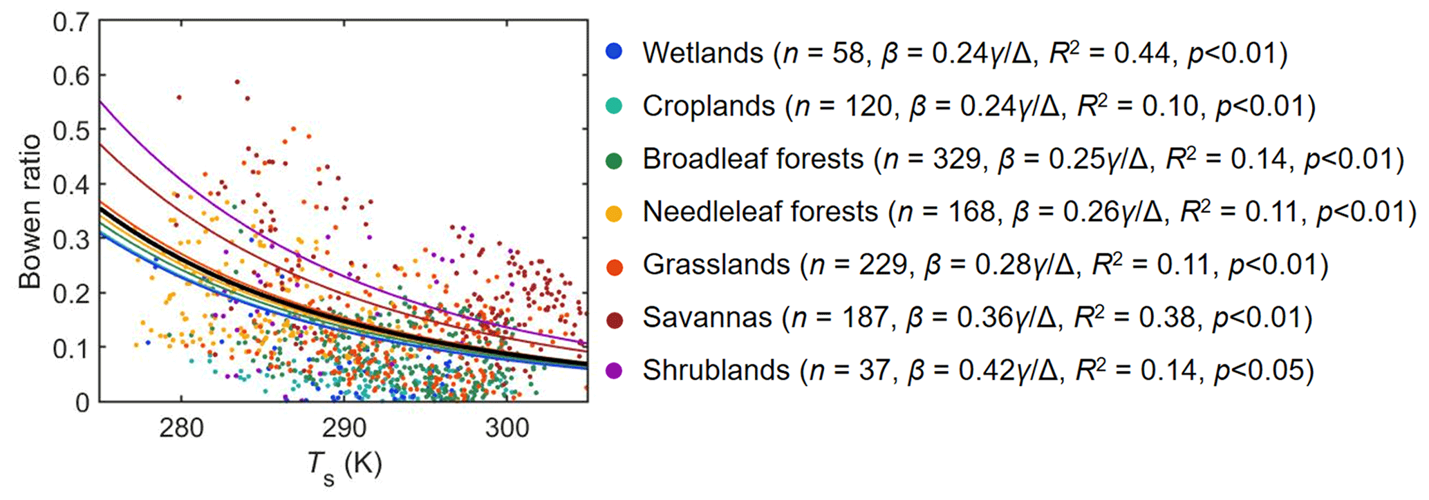
Figure 2 Relationship between Bowen ratio (β) and surface temperature (T_s) over saturated land surfaces. The thick black curve represents the fitted β–T_s relationship across all data points (i.e., n=1128, $\mathit{\beta }=\mathrm{0.27}\mathit{\gamma }/\mathrm{\Delta }$, R²=0.11, p<0.001), and the colored lines represent different biome types with the number of data points (n site-days) and fitted β–T_s relationship for each biome type shown in the legend.

To get an overview of how each of the energy fluxes varies with T_s, we first examine the maximum evaporation theory using the pooled data over all 1128 site-days (Fig. 3). Under this condition, the mean observed net shortwave radiation (R_sn) over all site-days is 176.6 W m⁻² and G is 1.0 W m⁻². Since R_sn is not directly dependent on T_s and G is negligibly small, the term R_sn minus G is held constant across the entire T_s range. With the increase of T_s, it is readily apparent that both outgoing and incoming longwave radiation (R_lo and R_li) steadily increase (see Sect. 2.2 for details about the coupling between R_lo and R_li), with R_lo increasing slightly faster than R_li, leading to a decreased net longwave radiation and thus a decreased R_n as T_s increases (Fig. 3). With this and the observed generic dependence of β on T_s ($\mathit{\beta }=\mathrm{0.27}\mathit{\gamma }/\mathrm{\Delta }$, Fig. 2), a maximum LE emerges along the T_s gradient that represents the interaction between decreasing R_n and increasing evaporative fraction as T_s increases. For the pooled dataset used here, the maximum LE (LE_max) is found to be 105.6 W m⁻² and the corresponding T_s is 294.7 K, both of which are very close to the averages computed from all daily flux site observations (i.e., LE_obs=102.4 W m⁻² and T_{s_obs}=292.3 K) (Fig. 3).

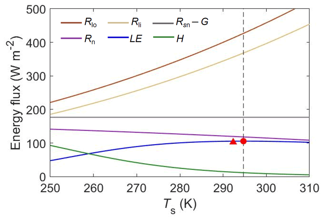
Figure 3 Variation of energy fluxes with T_s. Plot shows how the energy fluxes vary with T_s for a fixed value of R_sn−G at 176.6 W m⁻² (R_sn is the net shortwave radiation; see Eq. 4 in Sect. 2.2). The red dot indicates the maximum evaporation and the red triangle shows the observed evaporation. The T_s at which the maximum evaporation occurs is shown by the dashed vertical line.

Having demonstrated the overall concept, we next perform the detailed calculations using data for all individual site-days (Figs. 4–6). Using the same generic β dependence on T_s ($\mathit{\beta }=\mathrm{0.27}\mathit{\gamma }/\mathrm{\Delta }$), the LE_max estimated from the maximum evaporation model agrees very well with flux site observations, yielding an R² of 0.92, a root-mean-squared error (RMSE) of 14.6 W m⁻², and a mean bias of 1.6 W m⁻² (Fig. 4a). The performance of the maximum evaporation model improves slightly when the biome-specific model parameters are used (RMSE decreases to 14.1 W m⁻² and mean bias decreases to 1.4 W m⁻²; Fig. 4b). This result demonstrates that LE_max corresponds to the observed evaporation under well-watered conditions across a broad range of bio-climates. In fact, when the previously identified ocean surface β–T_s relationship is adopted, the maximum evaporation approach performs only slightly worse than those based on the calibrated β–T_s relationship over saturated lands, yielding an R² of 0.91, an RMSE of 14.8 W m⁻², and a mean bias of 2.8 W m⁻² (Fig. 4c).

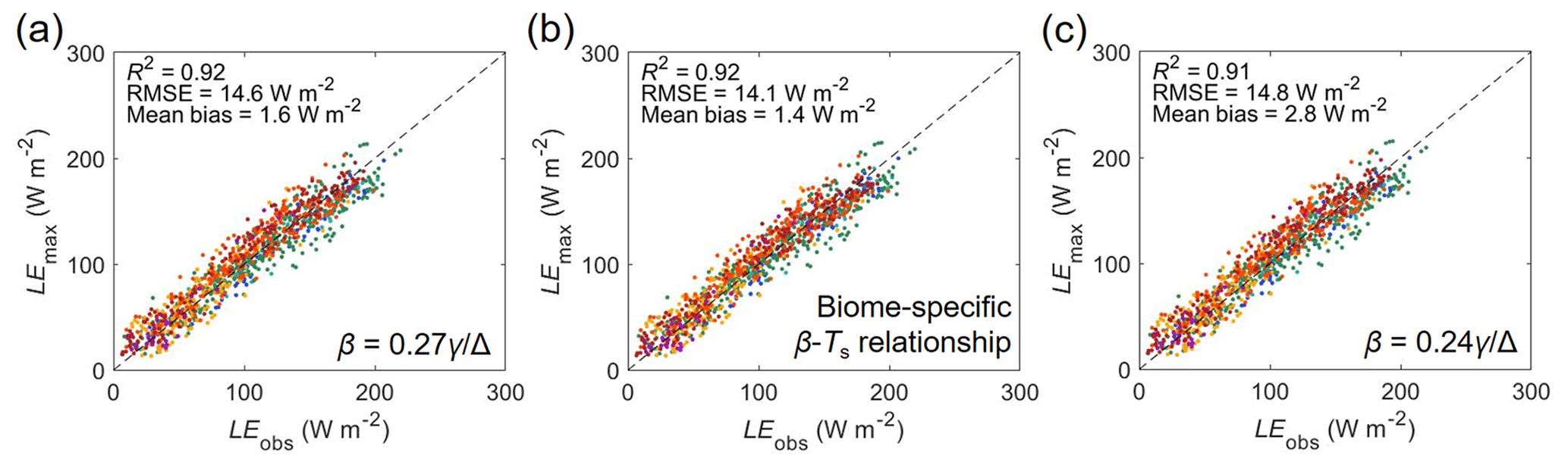
Figure 4 Comparison of the maximum evaporation and observed evaporation over saturated land surfaces using three different β–T_s relationships. (a) Generic land β–T_s relationship ($\mathit{\beta }=\mathrm{0.27}\mathit{\gamma }/\mathrm{\Delta }$, n=1128). (b) Biome-specific β–T_s relationships (per Fig. 2). (c) Ocean surface β–T_s relationship ($\mathit{\beta }=\mathrm{0.24}\mathit{\gamma }/\mathrm{\Delta }$, Yang and Roderick, 2019). The colors indicate different biome types (as provided in Fig. 1). The dashed black line indicates the 1:1 line.

We next test whether the maximum evaporation approach could recover T_s over the same saturated land surfaces. Similar to the test of LE, the three β–T_s relationships are respectively used. Results show that when the generic β–T_s relationship over land is used (i.e., $\mathit{\beta }=\mathrm{0.27}\mathit{\gamma }/\mathrm{\Delta }$), the T_s at which LE_max occurs corresponds reasonably well to the observed T_s, with an R² of 0.62, an RMSE of 4.3 K, and a mean bias of 0.3 K (Fig. 5a), indicating that the maximum evaporation approach is also able to recover T_s under saturated conditions. Again, the model's performance in recovering T_s increases slightly when the biome-specific β–T_s relationships are used (Fig. 5b). When the ocean surface β–T_s relationship is used, the model performs similarly in estimating the variability of T_s to that of the generic land β–T_s relationship (Fig. 5c). However, the ocean surface β–T_s relationship (Fig. 5c) results in a higher T_s mean bias compared to the β–T_s relationships obtained over land (Fig. 5a).

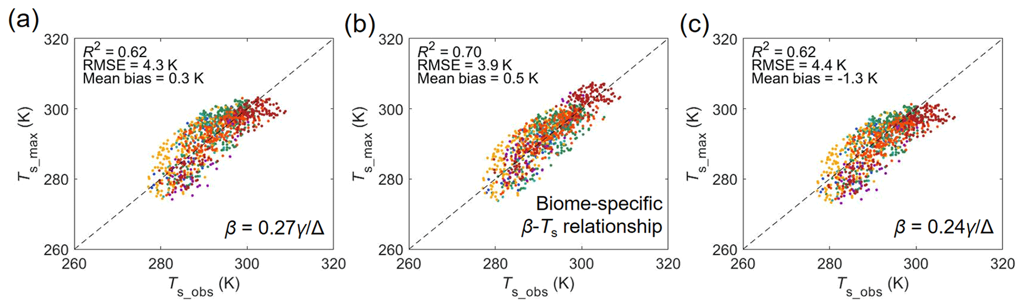
Figure 5 Comparison of the estimated and observed surface temperature over saturated land surfaces using three different β–T_s relationships. Comparison of estimated surface temperature (T_{s_max}) with flux site observations (T_{s_obs}). (a) Generic land β–T_s relationship ($\mathit{\beta }=\mathrm{0.27}\mathit{\gamma }/\mathrm{\Delta }$, n=1128). (b) Biome-specific β–T_s relationships (per Fig. 2). (c) Ocean surface β–T_s relationship ($\mathit{\beta }=\mathrm{0.24}\mathit{\gamma }/\mathrm{\Delta }$, Yang and Roderick, 2019). The colors indicate different biome types (as provided in Fig. 1). The dashed black line indicates the 1:1 line.

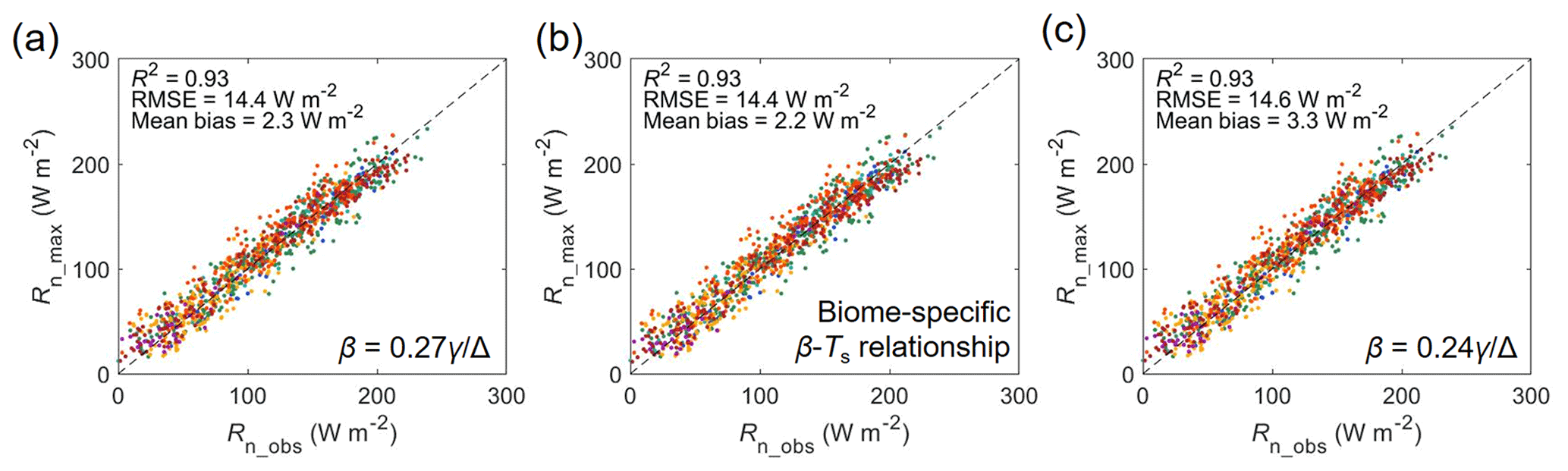
Figure 6 Comparison of the estimated and observed net radiation over saturated land surfaces using three different β–T_s relationships. Comparison of estimated net radiation (R_{n_max}) with flux site observations (R_{n_obs}). (a) Generic land β–T_s relationship ($\mathit{\beta }=\mathrm{0.27}\mathit{\gamma }/\mathrm{\Delta }$, n=1128). (b) Biome-specific β–T_s relationships (per Fig. 2). (c) Ocean surface β–T_s relationship ($\mathit{\beta }=\mathrm{0.24}\mathit{\gamma }/\mathrm{\Delta }$, Yang and Roderick, 2019). The colors indicate different biome types (as provided in Fig. 1). The dashed black line indicates the 1:1 line.

Different from most state-of-the-art evaporation models, the maximum evaporation approach does not rely on observed R_n (or independent R_n estimates) as model input but estimates R_n as a result of the R_n–T_s–E interaction. Here, we also test the estimated R_n calculated using the maximum evaporation approach as the discrepancy between LE_max and LE_obs is mainly caused by the slight difference between T_{s_max} and T_{s_obs} that leads to different R_lo and R_li (and thus a different R_n) being used in the calculation of LE_max. It should be noted that since the observed shortwave radiation is used in the maximum evaporation model, validation of R_n is essentially the same as the validation of net longwave radiation. We find that the maximum evaporation model could satisfactorily reproduce the observed R_n when the generic land β–T_s relationship is used, as indicated by an R² of 0.93, an RMSE of 14.4 W m⁻², and a mean bias of 2.3 W m⁻² (Fig. 6a). Using biome-specific β–T_s relationships or the ocean surface β–T_s relationship does not considerably increase or decrease the model's performance in estimating R_n (Fig. 6b and c).

4 Discussion

Taking R_n and/or T_s (or near-surface air temperature) to be independent forcings has long been identified as a scientific concern in the use of evaporation models (Milly, 1991; Monteith and Unsworth, 2013; Philip, 1987). Here, we test a maximum evaporation theory developed over the global ocean surface that addresses this concern by explicitly acknowledging the interdependence between radiation, surface temperature, and evaporation (Yang and Roderick, 2019). Our new results show that there exists a maximum evaporation along the T_s gradient that corresponds to the observed evaporation under saturated conditions over land (Figs. 3 and 4). In addition, the T_s at which LE_max occurs also corresponds reasonably well to the observed T_s (Figs. 3 and 5). These results mirror those found previously over the global ocean (Yang and Roderick, 2019). This is not a surprise since the basic principles are the same for a wet land surface and the ocean surface. These results suggest that saturated land surfaces behave essentially the same as ocean surfaces and imply that LE_max is a natural attribute of the land surface when water availability does not limit evaporation.

A key assumption involved in the maximum evaporation model is that β decreases with the increase of T_s under saturated conditions. Nevertheless, this key assumption that β decreases with the increase of T_s under saturated conditions has been extensively validated in previous studies based on theoretical relationships (Philip, 1987; Priestley and Taylor, 1972; Slatyer and McIlroy, 1961; Lhomme, 1997) and in situ observations (Andreas et al., 2013; Guo et al., 2015; Yang and Roderick, 2019; also see Fig. S3). Moreover, our results also found this held over saturated lands (Fig. 2). The original maximum evaporation study reported that $\mathit{\beta }=\mathrm{0.24}\mathit{\gamma }/\mathrm{\Delta }$ over global ocean surfaces (Yang and Roderick, 2019). Here, we find the generic land surface coefficient increases to 0.27 (i.e., $\mathit{\beta }=\mathrm{0.27}\mathit{\gamma }/\mathrm{\Delta }$, Fig. 2), which indicates a slightly higher β over wet vegetated land than that over the ocean surface for the same T_s. This is biophysically reasonable, as the stoma of plant leaves represents an additional resistance to vapor transfer between the land and the atmosphere (Swann et al., 2016; Yang et al., 2019), which lowers the ability of a generic vegetated surface to convert available energy into LE for a given T_s, compared to open water surfaces. In addition, different surface roughness can also lead to different β–T_s relationships between the land and the ocean. Compared with the ocean surface that shows a tight β–T_s relationship (Yang and Roderick, 2019), the β–T_s relationships over saturated vegetated land are relatively weak with considerable scatter (Fig. 2). This data scatter could be caused by several reasons. First, the observations by EC towers can be a source of uncertainty. This is threefold, including (i) the quality of the observations, (ii) the footprint within each EC tower (possibly) being heterogeneous (Lee et al., 2004; Paw et al., 2000), and (iii) whether or not the selected days are truly non-water-limited (however, see Fig. S4). Second, as is seen in Fig. 2, different biome types exhibit different β–T_s relationships. This can be caused by different surface resistance and roughness between biome types and even between sites. Nevertheless, these data-based limitations only have limited impacts on the model performance, as similar performance is obtained using both the generic β–T_s relationship (i.e., $\mathit{\beta }=\mathrm{0.27}\mathit{\gamma }/\mathrm{\Delta }$) and biome-specific β–T_s relationships (Fig. 4). Third, wind speed could be another factor that leads to the scatter. For the same surface roughness, a different wind speed will lead to a different aerodynamic resistance and therefore a different β. However, this effect is usually very small, as demonstrated by the long-standing similarity theory (the transfer of mass and heat share the same aerodynamic process in the lower atmospheric boundary layer; Monin and Obukhov, 1954). In fact, our findings that one can make a reasonable estimate of LE using a generic land or ocean β–T_s relationship instead of a site-specific relationship (Fig. 4) imply that R_n is the primary determinant of LE over saturated surfaces. As evaporation tends to operate at its maximum strength, sensible heat (and β) are usually very small over warm saturated land surfaces. As a result, once R_n can be accurately determined, any reasonable β–T_s relationship (Fig. 2) would result in a satisfactory LE estimate (Figs. 4 and S5). Our result highlighted in Fig. 3 shows that R_n (and hence LE) is only a weak function of T_s and this explains why one can obtain an accurate estimate of LE using a generic β–T_s relation. However, the same logic also leads to the conclusion that an accurate β–T_srelationship will be necessary to estimate T_s, since T_s is very sensitive to changes in LE (Fig. 3). In this regard, using the land β–T_s relationships (preferably site-specific relations) is preferable to a generic ocean surface relation (Fig. 5). To further demonstrate the above points, we conduct an uncertainty test by varying the coefficient m in the β–T_s relationship in Fig. S6. We find that when m ranges from 0.18 to 0.36 (all other forcings as per Fig. 3), the change in estimated LE_max is only 9 W m⁻² (101.7–110.7 W m⁻²), whereas the change in estimated T_{s_max} is as high as 11.6 K (287.9–299.5 K).

Besides the data scattering that leads to an uncertainty in the β–T_s relationships, there are also uncertainties associated with (i) parameterization of the longwave coupling and (ii) selection of non-water-stressed observations in the current study. In the maximum evaporation approach, the coupling between outgoing and incoming longwave radiation is calculated using the temperature difference between the surface and an effective radiating height in the atmosphere (ΔT) and is parameterized as a function of shortwave atmospheric transmissivity and geographic latitude. However, the shortwave atmospheric transmissivity is primarily affected by aerosols, while the longwave transmissivity is mainly affected by the concentration of greenhouse gases. Nevertheless, here we only deal with wet conditions, under which the vapor concentration of the atmosphere is also relatively high and more aerosols would favor the development of more clouds that simultaneously affect both shortwave and longwave radiation. We suspect that this underlies the excellent performance of Eq. (5) in estimating ΔTat the flux sites (Fig. S2). To further evaluate that conclusion, we additionally evaluate the estimated longwave radiation against four global products (i.e., ERA5, Hersbach et al., 2020; CERES, Kato et al., 2018; the Princeton global forcing data, Sheffield et al., 2006; the GLDAS global forcing data, Rodell et al., 2004) and compare our longwave estimates with other two semi-empirical models (i.e., Brutsaert, 1975; Shakespeare and Roderick, 2021). The results show our ΔT-based approach to be the best performer across a wide range of conditions when the surface is wet (Fig. S7). In addition, we further note that our maximum evaporation model is only tested at the daily timescale (Figs. 4–6) and longer (Fig. 3). In particular, for timescales shorter than that (e.g., hourly), the diurnal cycle of E can be very different for ocean and land surfaces (Kleidon and Renner, 2017). In addition, the parameterization of the coupling between incoming and outgoing longwave radiation via Eq. (5) requires a timescale that is long enough to allow the surface heat fluxes to be fully redistributed through the atmospheric column (Yang and Roderick, 2019). At sub-daily scales, Eq. (5) is likely invalid because R_lo usually exhibits a larger diurnal range than R_li during a typical cloudless day (Monteith and Unsworth, 2013). For even longer periods, especially for assessing the impacts of climate change, the relationship between shortwave and longwave radiation used herein may also be invalid, as we expect this relationship to evolve with anthropogenic climate change.

As for the selection of non-water-stressed evaporation observations from global EC towers, we rely largely on the same selection criteria used in a previous study (Maes et al., 2019). However, these selection criteria are somewhat subjective and represent a compromise between better data quality and more data samples. As a result, the selected site-days are not necessarily non-water-limited. Nevertheless, varying the selection criteria (changing the thresholds) of non-water-stressed evaporation only resulted in minor changes in the overall model performance (Fig. S4), which suggests that the uncertainties in the selection of non-water-stressed evaporation observations would not materially change our conclusion.

The ability of the maximum evaporation model to recover LE and T_s over vegetated lands under saturated conditions has an important implication for the estimation of potential evaporation, which is a central concept in hydrology and agriculture (and especially in irrigation). The underlying idea of E_P is straightforward – it is the evaporation that would occur with an unlimited supply of water. However, the formal physical definition of E_P has been widely debated in the literature (Brutsaert, 2005; Donohue et al., 2010; Granger, 1989; Nash, 1989) and the calculation of E_P using conventional evaporation models is problematic (Aminzadeh et al., 2016; Roderick et al., 2015). The key scientific issue is that the meteorological forcing variables observed over actual surfaces are generally not equivalent to the meteorological variables that would be measured over a hypothetical surface with an unlimited water supply. Compared with existing evaporation models, the maximum evaporation model presented here requires fewer meteorological variables than existing approaches (but performs similarly with existing approaches under wet conditions; see Fig. S8 for details). This new approach only requires the incoming and reflected solar radiation, a relationship that describes a decreasing dependence of β on T_s, and a relation for the coupling of the incoming and outgoing longwave radiation. With these modest requirements, LE_max naturally follows from the physical interdependence between radiation, surface temperature, and evaporation. These features suggest that the maximum evaporation model can be used to make a strictly independent estimate of E_P. In fact, the maximum evaporation formulation directly maps to one particular definition of E_P that was proposed by Brutsaert (2015) as “the maximum evaporation that would occur over real surfaces with the actual solar forcing and a prescribed Bowen ratio”.

5 Conclusions

In this study, we test a maximum evaporation theory that explicitly acknowledges the interdependence between radiation, surface temperature, and evaporation over saturated land surfaces. Validated against flux site observations, we show that the maximum evaporation approach could recover the observed evaporation across a broad range of bio-climates. In comparison, although the model is also able to reasonably recover the observed T_s, the model's performance in recovering T_s is not as good as that for LE. Nevertheless, this does not materially lead to larger errors in LE estimates, as we additionally demonstrate that LE is not sensitive to T_s changes. The overall good performance of the maximum evaporation approach over saturated surfaces implies the method's great potential for use in estimating potential evaporation. To calculate E_P in practice using the maximum evaporation approach, a detailed site-specific (or biome-specific) β–T_s relationship (e.g., Fig. 2) would be favorable; otherwise, a generic default β–T_s relationship ($\mathit{\beta }=\mathrm{0.27}\mathit{\gamma }/\mathrm{\Delta }$ or even $\mathit{\beta }=\mathrm{0.24}\mathit{\gamma }/\mathrm{\Delta }$) can also lead to a reasonable E_P estimate that remains consistent with the E_P definition by Brutsaert (2015). Table S2 gives a working example of applying the maximum evaporation model for E_P estimation.