Modelling the artificial forest (Robinia pseudoacacia L.) root–soil water interactions in the Loess Plateau, China

Plant root–soil water interactions are fundamental to vegetation–water relationships. Soil water availability and distribution impact the temporal–spatial dynamics of roots and vice versa. In the Loess Plateau (LP) of China, where semi-arid and arid climates prevail and deep loess soil dominates, drying soil layers (DSLs) have been extensively reported in artificial forestland. While the underlying mechanisms that cause DSLs remain unclear, they hypothetically involve root–soil water interactions. Although available root growth models are weak with respect to simulating the rooting depth, this study addresses the hypothesis of the involvement of root–soil water interactions in DSLs using a root growth model that simulates both the dynamic rooting depth and fine-root distribution, coupled with soil water, based on cost–benefit optimization. Evaluation of field data from an artificial black locust (Robinia pseudoacacia L.) forest site in the southern LP positively proves the model's performance. Further, a long-term simulation, forced by a 50-year climatic data series with varying precipitation, was performed to examine the DSLs. The results demonstrate that incorporating the dynamic rooting depth into the current root growth models is necessary to reproduce soil drying processes. The simulations revealed that the upper boundary of the DSLs fluctuates strongly with infiltration events, whereas the lower boundary extends successively with increasing rooting depth. Most infiltration was intercepted by the top 2.0 m layer, which was the most active zone of infiltration and root water uptake. Below this, the percentages of fine roots (5.0 %) and water uptake (6.2 %) were small but caused a persistently negative water balance and consequent DSLs. Therefore, the proposed root–water interaction approach succeeded in revealing the intrinsic properties of DSLs; their persistent extension and the lack of an opportunity for recovery from the drying state may adversely affect the implementation of artificial afforestation in this region as well as in other regions with similar climates and soils.

1 Introduction

Plant roots are a significant pathway in the soil–plant–atmosphere continuum (SPAC), which connects the above-ground parts of the plant and the soil environment (Feddes et al., 2001; Mencuccini et al., 2019) by extracting water from the soil to meet the evaporation demand of the canopy. This soil water uptake process is regulated by root profile properties, which are highly dynamic in response to variable soil water conditions (Schenk and Jackson, 2002; Fan et al., 2017). In particular, forest root structures are rather complex (e.g. have woody coarse roots for anchoring and non-woody fine roots for absorption) and enable diverse water exploration strategies for adaptation to changing environments (Mulia and Dupraz, 2006; Ivanov et al., 2012; Sivandran and Bras, 2013; Brunner et al., 2015). For example, in order to increase water uptake, forests tend to grow more roots in the wetter soil layers (i.e. root hydrotropism) or develop deep roots to extract deeper water resources (including deep soil water and groundwater) (Maeght et al., 2013; Bardgett et al., 2014; Phillips et al., 2016). The investigation also indicated that forest stands develop a complicated morphological distribution of roots and diverse root water uptake strategies to adapt to the diverse soil water status conditions (Germon et al., 2020; Knighton et al., 2020). Therefore, plant root–soil water interaction is a key issue for understanding the forest–water relationship, which is inevitably an important part of ecohydrological models, fundamentally for plant water uptake (Smithwick et al., 2014).

Plant water uptake is usually taken as a sink term in water movement equations (Feddes et al., 2001; Clark et al., 2015). The sink term is expressed as a function of the morphological and hydrological traits of the roots and soils. Morphologically, the root profile contains two primary features, rooting depth and vertical distribution (Warren et al., 2015), which are commonly included in most current root uptake models. These features are usually considered static in most of the available hydrological and terrestrial biospheric models (Luo et al., 2003; Warren et al., 2015). The maximum rooting depths are generally assumed to be static values which may differ from the plant functional types (Ostle et al., 2009). Meanwhile, the vertical root distribution is represented as an empirical function of root length density to soil depth over the root domain (Jackson et al., 1996; Zuo et al., 2004; Sivandran and Bras, 2012), which describes the morphological features of roots statically. These simplifications of the root features allow for ease in practical applications to simulate the root uptake process. However, it is increasingly recognized that efforts should be made to account for root dynamics, especially when the coupling effects between plant growth and water availability are considered (Warren et al., 2015).

The dynamic roots indicate that the hydrological or terrestrial biospheric models simulate growing roots under changing environmental conditions, for example, soil water status. This is further incorporated into the root water uptake models. In these process models, the dynamic root profiles may be accounted for by either the changing rooting depth (Gayler et al., 2014; Hashemian et al., 2015; Christina et al., 2017; Liu et al., 2020) or the root density distribution (Schymanski et al., 2008; Wang et al., 2016; P. Wang et al., 2018; Drewniak, 2019; Niu et al., 2020), which is not sufficient to describe the dynamic root adaptation to changing environmental conditions (Rudd et al., 2014). The rooting depth, root density distribution, soil water quantity, and soil water spatial distribution are interrelated, and their coupling should be reflected in the root water uptake modelling (Warren et al., 2015). Sakschewski et al. (2021) reviewed the root growth approaches in the current Earth system models and concluded that “none of those studies have acknowledged resource investment, timing and physical constraints of tree rooting depth within a competitive environment”. Therefore, they implemented variable rooting strategies and dynamic root growth into the LPJmL4.0 model. Their results indicated that “variable tree rooting strategies are key for modelling the distribution, productivity and evapotranspiration of tropical evergreen forests” in tropical South America. In their model, the maximum rooting depth is estimated by the tree height through a logistic growth function, and the vertical distribution of the fine roots follows a shape function. Notably, the interactions between plant roots and soil water were not considered.

To meet their water requirement, plants tend to develop more roots in water-rich zones (Germon et al., 2020). Within the root system, soil water is conveyed up to the above-ground parts through fine roots (<2 mm in diameter) and coarse roots (>2 mm diameter), the former for water uptake and the latter for water transport (Jackson et al., 1997; Smithwick et al., 2014). Fine roots are developed on coarse roots, together constituting a hydraulic architecture, creating structural relationships for water transport (Smithwick et al., 2014; Chen et al., 2019). According to the pipe model theory (Lehnebach et al., 2018), for denser fine roots to take up more soil water, coarser roots are required to maintain the hydraulic transport capacity, especially for deeper extension. Balancing the cost of biomass allocation to coarse or fine roots and the benefit of the water taken up is a great ability of plants which live under water-stressed conditions (Guswa, 2008). Mathematical optimization methods have been widely implemented in previous studies to estimate the optimal root profiles (Kleidon and Heimann, 1998; Collins and Bras, 2007; Guswa, 2008; Schymanski et al., 2008, 2009; Yang et al., 2016). Nonetheless, optimization efforts for root dynamic processes remain limited. The coupled effects of root growth and soil water should be the fundamentals in the optimization approach. An optimization method will be surely beneficial for simultaneously estimating the dynamics of rooting depth and fine-root distribution.

A drying soil layer is defined as a soil layer with a soil water content between stable field capacity and permanent wilting point (Wang et al., 2011). This is a phenomenon of concerned and has been widely studied in the Loess Plateau of Northwest China. Huang and Shao (2019) reviewed the studies on drying soil layers in the Loess Plateau over the past decades; this review indicated that drying soil layers prevail in the artificial forestlands in the region and develop as the stand ages. It is generally believed that drying soil layers are caused by limited rainfall infiltration and improper afforestation; however, the underlying mechanisms remain unclear and require exploration (Shao et al., 2018). Although rainfall is insufficient in the semi-arid and arid climates in the Loess Plateau, the thick loess soils store significant quantities of water for potential plant use. When water stress occurs in the upper soil layer due to insufficient infiltration, high atmospheric demand due to the aridity may cause plants to develop roots for the use of deeper soil water (Pierret et al., 2016). Thus, root–water interactions may play a key role in the occurrence and development of drying soil layers.

Many in situ investigations have reported that a drying soil layer has developed extensively in forests of black locust (Robinia pseudoacacia L.), which is the most popular and deep-rooted afforestation species in Loess Plateau (Deng et al., 2016; Jia et al., 2017b; Liang et al., 2018; Wu et al., 2021). Thus, the occurrence and evolution of a drying soil layer in this forestland are worthy of discussion. Hence, this study aimed to (1) develop a coupled soil water–root growth model based on the cost–benefit theory, which can simultaneously adjust root distribution and rooting depth in the root water uptake model, and (2) reveal the black locust root–soil water interactions throughout the soil profile, based on a long-term simulation, to address the drying soil layer issues in this region.

2 Materials and methods

2.1 Model development

2.1.1 General description of the ecohydrological model

Fundamentally, this ecohydrological model is an integration of different components from the Soil and Water Assessment Tool (SWAT) (Neitsch et al., 2011; Arnold et al., 2012) and the Community Land Model version 4.5 (CLM4.5) (Oleson et al., 2013) (Fig. 1). On this basis, root growth and root uptake modules were modified. Furthermore, an optimization approach was introduced to simulate the coupled effects of root growth and soil water dynamics.

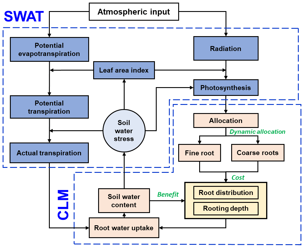
Figure 1 The model structure integrated from the SWAT (blue boxes) and CLM (light orange boxes) components. The root growth module is highlighted in yellow, and the descriptions of the dynamic fine-root distribution and rooting depth approach are illustrated using green text.

Hydrologically, surface process modules, for example, simulating evaporation, transpiration, canopy interception, and runoff, follow the SWAT model, which is detailed in its theoretical document (Neitsch et al., 2011). The subsurface hydrological modules, primarily the soil water movement, adopted the 1-D Richards' equation. It is solved numerically following the finite difference scheme used in CLM4.5 (Oleson et al., 2013).

Biologically, modules for the above-ground parts, for example, plant phenology, leaf area index (LAI) development, and biomass accumulation, are adopted from SWAT (Neitsch et al., 2011) and CLM4.5 (Oleson et al., 2013). The module for the below-ground part, the root growth model, simulates root growth following CLM4.5 which, in turn, adopts the approaches from process simulation directly from the implementation in the Biome-BGC (Biome BioGeochemical Cycles) model (Thornton et al., 2002). See the Supplement for more information on the detailed model descriptions. In CLM4.5, the roots are categorized into coarse and fine. The rooting depth is presented as a static value, and the fine-root distribution follows a static shape function which defines the root density over the soil profile.

The root–water interaction is integrated into the root uptake model, which uses the rooting depth and fine-root distribution as input and acts as a sink term in the Richards' equation. Soil water imposes water stress on the root growth. The cost of biomass invested in coarse and fine roots and the benefit of water uptake were optimized through a cost–benefit function.

The following sections will describe three root growth approaches in a stepwise manner: (1) the static root distribution approach implemented in CLM4.5, which assumes a static rooting depth of the coarse roots and a static distribution of fine roots (Oleson et al., 2013); (2) the approach that assumes a dynamic distribution of fine roots but a static rooting depth (Drewniak, 2019); and (3) the approach proposed in this study that assumes a dynamic distribution of fine roots and a dynamic rooting depth of coarse roots. These three root growth modelling approaches are incorporated into the ecohydrological model mentioned above for a comparison of their performances.

2.1.2 Static distributions of coarse and fine roots

In this approach, a static exponential function expresses the root fractions in different soil layers (Zeng, 2001):

$$\begin{array}{}\text{(1)}& {\mathrm{fr}}_i=\left\{\begin{array}{ll}\mathrm{0.5}\left[\exp \left(-r_a{z}_{h,i-\mathrm{1}}\right)+\exp \left(-r_b{z}_{h,i-\mathrm{1}}\right)\right.& \\ \left.-\exp \left(-r_a{z}_{h,i}\right)-\exp \left(-r_b{z}_{h,i}\right)\right]& \mathrm{1}\le i<n\\ \mathrm{0.5}\left[\exp \left(-r_a{z}_{h,i-\mathrm{1}}\right)+\exp \left(-r_b{z}_{h,i-\mathrm{1}}\right)\right]& i=n\end{array}\right.,\end{array}$$

where i is the sequential number of soil layers, n is the total number of soil layers in the rooting zone, z_h,i is the depth of soil layer i, and r_a and r_b are two shape parameters. The shape parameters can be obtained by fitting to the observations for different plant types and are set as 4.8 and 0.8 according to fine-root sampling in this study (see Sect. 2.2.4) respectively (Oleson et al., 2013).

2.1.3 Dynamic distribution of fine roots

This approach assumes that newly assimilated biomass to the below-ground parts is allocated to develop fine and coarse roots with a static ratio. In general, there is a linear relationship between the carbon mass and biomass (Niu et al., 2020). Therefore, the term “carbon” will be used in the following text to refer to the biomass of different plant components. Within the present rooting depth (which is static over the simulation period), the fine roots are distributed over the soil depth according to the soil water content. In each soil layer i, the fine-root carbon increment is updated at each time step, as follows:

$$\begin{array}{}\text{(2)}& {\mathrm{FR}}_{i,t}={\mathrm{FR}}_{i,t-\mathrm{1}}+\mathrm{\Delta }{\mathrm{FR}}_{i,t},\end{array}$$

where ${\mathrm{FR}}_{i,t-\mathrm{1}}$ (g m⁻² d⁻¹) is the fine-root carbon of soil layer i during the previous time step, and ΔFR_i,t (g m⁻² d⁻¹) is the newly allocated carbon to fine roots of soil layer i at time t. ΔFR_i,t is modified by the soil water content as follows:

$$\begin{array}{}\text{(3)}& \mathrm{\Delta }{\mathrm{FR}}_{i,t}=\mathrm{\Delta }\mathrm{FR}\cdot {\displaystyle \frac{{\mathrm{THK}}_i{\mathrm{REW}}_i}{\sum _{i=\mathrm{1}}^n\left({\mathrm{THK}}_i{\mathrm{REW}}_i\right)}},\end{array}$$

where ΔFR is the newly assimilated carbon allocated to total fine roots (g m⁻² d⁻¹), n is the total number of soil layers in the rooting zone, THK_i is the soil layer thickness of soil layer i (cm), and REW_i is the relatively effective soil water content (i.e. soil water availability). REW_i is calculated as follows:

$$\begin{array}{}\text{(4)}& {\mathrm{REW}}_i={\displaystyle \frac{\mathit{\theta }-{\mathit{\theta }}_{\mathrm{wp}}}{{\mathit{\theta }}_{\mathrm{fc}}-{\mathit{\theta }}_{\mathrm{wp}}}},\end{array}$$

where θ is the soil water content (cm³ cm⁻³), and the subscripts “wp” and “fc” indicate the soil water content at the wilting point and field capacity respectively.

The fine-root fraction in each soil layer i is then calculated:

$$\begin{array}{}\text{(5)}& {\mathrm{fr}}_i={\displaystyle \frac{{\mathrm{FR}}_{i,t}}{\sum _{i=\mathrm{1}}^n{\mathrm{FR}}_{i,t}}}.\end{array}$$

2.1.4 Dynamic distributions of coarse and fine roots

This approach assumes that both the rooting depth of coarse roots and the distribution of fine roots change with soil water. In formulating the growth of the coarse and fine roots, the newly allocated biomass/carbon for the below-ground part is optimally allocated to the roots based on a cost–benefit function that will be described in detail.

(1) Carbon allocation between the coarse and fine roots

The cost is defined as the amount of carbon invested to grow coarse/fine roots. In constructing the coarse-root and fine-root systems, the pipe model theory (PMT; Shinozaki et al., 1964) was adopted. Lehnebach et al. (2018) summarized “the essence of the PMT concept” as “a unit amount of leaves is provided with a pipe whose thickness or cross-sectional area is constant. The pipe serves both as the vascular passage and as the mechanical support and runs from the leaves to the stem through all intervening strata.” The relationship between the leaf and stem can be established quantitatively based on the PMT and can be extended to the below-ground parts of the plants (Chen et al., 2019). For roots, the relationships have been established in analogue form and validated against some databases (Carlson and Harrington, 1987; Richardson and Dohna, 2003).

Delineating the soil profile into adjacent soil layers which correspond to the numerical solution of the Richards' equation, the equations for modelling the root growth are also written regarding the discrete soil layers (Fig. 2c).

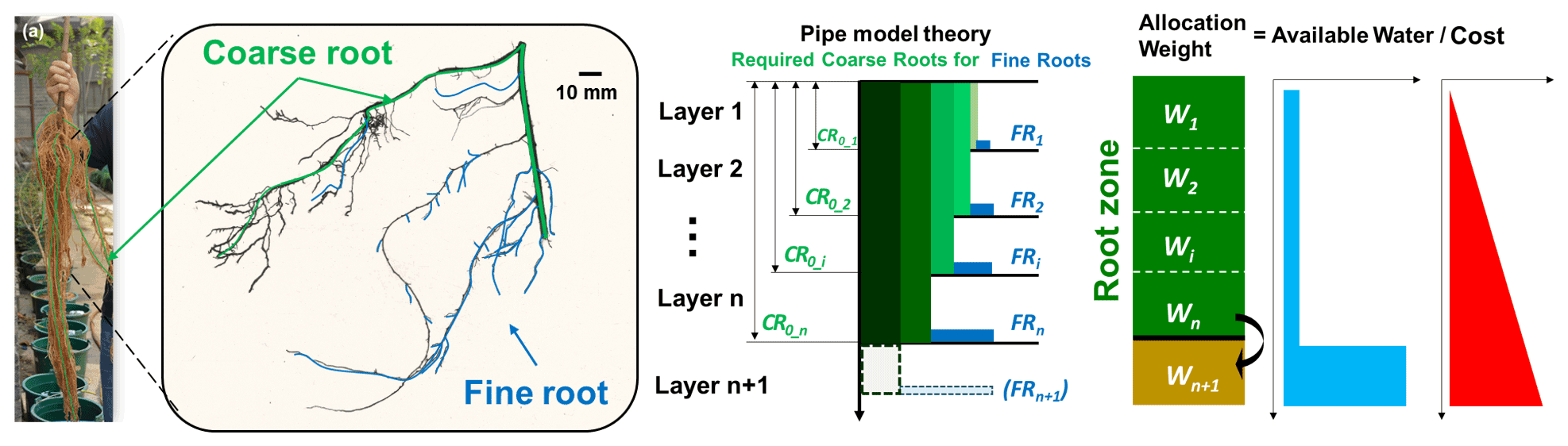
Figure 2 (a) Black locust root system obtained from an experimental pot; (b) scanned image of one root segment consisting of coarse and fine roots; (c) schematic description of pipe model theory adopted for coarse and fine roots; (d) weighting factors for carbon allocation and conceptualized benefit (available soil water for uptake) and cost (carbon investment).

The carbon amount for coarse and fine roots should be maintained as

$$\begin{array}{}\text{(6)}& {\mathrm{CR}}_{{\mathrm{0}}_i}=\mathit{\rho }\cdot Z_i\cdot k_A\cdot {\mathrm{FR}}_i,\end{array}$$

where ${\mathrm{CR}}_{{\mathrm{0}}_i}$ is the equivalent carbon for coarse roots in the zone between the ground surface and bottom of soil layer i, FR_i is the carbon for fine roots within soil layer i, ρ is the mass density of coarse roots (g cm⁻³), Z_i is the depth from the surface to the bottom of soil layer i (cm), and k_A is a constant which can be determined from field observations (see Sect. 2.3.2).

For an increment of carbon for fine roots within soil layer i, a corresponding increment of carbon for coarse roots is needed and can be derived from Eq. (6):

$$\begin{array}{}\text{(7)}& \mathrm{\Delta }{\mathrm{CR}}_{{\mathrm{0}}_i}=\mathit{\rho }\cdot Z_i\cdot k_A\cdot \mathrm{\Delta }{\mathrm{FR}}_i.\end{array}$$

Notably, there is no increment of carbon for coarse roots if the available coarse roots are sufficient to support the new fine roots, as discussed later.

The increments of carbon for fine and coarse roots were then summed over the root profile:

$$\begin{array}{}\text{(8)}& {\displaystyle }& {\displaystyle }\mathrm{\Delta }\mathrm{CR}=\sum _{\mathrm{1}}^n\mathrm{\Delta }{\mathrm{CR}}_{{\mathrm{0}}_i},\text{(9)}& {\displaystyle }& {\displaystyle }\mathrm{\Delta }\mathrm{FR}=\sum _{\mathrm{1}}^n\mathrm{\Delta }{\mathrm{FR}}_i.\end{array}$$

The sum of the newly allocated carbon for fine and coarse roots is equal to that allocated to the below-ground part ΔTR:

$$\begin{array}{}\text{(10)}& \mathrm{\Delta }\mathrm{FR}+\mathrm{\Delta }\mathrm{CR}=\mathrm{\Delta }\mathrm{TR}.\end{array}$$

Two respective ratios are defined for fine and coarse roots as follows:

$$\begin{array}{}\text{(11)}& K_{\mathrm{FR}}={\displaystyle \frac{\mathrm{\Delta }\mathrm{FR}}{\mathrm{\Delta }\mathrm{CR}+\mathrm{\Delta }\mathrm{FR}}},K_{CR}={\displaystyle \frac{\mathrm{\Delta }\mathrm{CR}}{\mathrm{\Delta }\mathrm{CR}+\mathrm{\Delta }\mathrm{FR}}}.\end{array}$$

(2) Spatial distribution of new fine and coarse roots

Potentially, more fine roots develop in wetter soil zones in order to gain more water and to reduce water stress as much as possible. It is fundamentally recognized that penetration into deeper soil requires carbon for the fine roots, as well as the corresponding coarse roots; the potential benefit can be more water uptake from the deeper soil. The basic principle for the distribution of the roots, either fine only or both coarse and fine, is that an optimal distribution of new roots helps to gain as much water as possible (Fig. 2d).

Thus, the distribution of fine roots is influenced by a cost–benefit ratio, which is defined as follows:

$$\begin{array}{}\text{(12)}& W_i={\displaystyle \frac{{\mathrm{REW}}_i}{{\mathrm{CFR}}_i}},\end{array}$$

where W_i is the cost–benefit ratio in soil layer i, and the benefit is presented by REW_i, as defined previously. CFR_i is defined as the marginal carbon cost of fine roots:

$$\begin{array}{}\text{(13)}& {\mathrm{CFR}}_i={\displaystyle \frac{\partial \left(\mathrm{\Delta }{\mathrm{CR}}_{{\mathrm{0}}_i}+\mathrm{\Delta }{\mathrm{FR}}_i\right)}{\partial \mathrm{\Delta }{\mathrm{FR}}_i}}=\mathit{\rho }\cdot Z_i\cdot k_A+\mathrm{1}.\end{array}$$

Combining Eqs. (13) and (12),

$$\begin{array}{}\text{(14)}& W_i={\displaystyle \frac{{\mathrm{REW}}_i}{\mathit{\rho }\cdot Z_i\cdot k_A+\mathrm{1}}}.\end{array}$$

Replacing REW_i with W_i in Eq. (3), the fraction of new fine roots in the soil layer i becomes

$$\begin{array}{}\text{(15)}& \mathrm{\Delta }{\mathrm{FR}}_i=\mathrm{\Delta }\mathrm{FR}\cdot {\displaystyle \frac{{\mathrm{THK}}_i{W}_i}{\sum _{i=\mathrm{1}}^m\left({\mathrm{THK}}_i{W}_i\right)}}.\end{array}$$

Updating the fine-root fractions using Eq. (7), the demand for coarse roots that can meet the hydraulic transport demand for the fine roots within and below soil layer i is

$$\begin{array}{}\text{(16)}& {\mathrm{CRP}}_i=\sum _{j=i}^n{\mathrm{CR}}_{{\mathrm{0}}_i,\mathrm{NEW}}=\sum _{j=i}^n\mathit{\rho }\cdot Z_i\cdot k_A\cdot \left({\mathrm{FR}}_i+\mathrm{\Delta }{\mathrm{FR}}_i\right).\end{array}$$

Comparing the demand for and current storage of coarse roots, the coefficient of the coarse-root carbon increment regarding the soil layer i is calculated as

$$\begin{array}{}\text{(17)}& {\mathit{\beta }}_i={\displaystyle \frac{\max \left({\mathrm{CRP}}_i-{\mathrm{CR}}_i,\mathrm{0}\right)}{\sum _{i=\mathrm{0}}^n\max \left({\mathrm{CRP}}_i-{\mathrm{CR}}_i,\mathrm{0}\right)}}.\end{array}$$

According to Eq. (11), the increment of carbon for the coarse roots with respect to each soil layer is then calculated as

$$\begin{array}{}\text{(18)}& \mathrm{\Delta }{\mathrm{CR}}_i=\mathrm{\Delta }\mathrm{TR}\cdot K_{\mathrm{CR}}\cdot {\mathit{\beta }}_{C_i}.\end{array}$$

(3) Rooting depth extension

To calculate the rooting depth extension via optimization, the target function S_m is defined as follows:

$$\begin{array}{}\text{(19)}& S_m=\sum _{i=\mathrm{1}}^m\left({\mathrm{THK}}_i\cdot {\mathrm{fr}}_i\cdot {\mathrm{REW}}_i\right).\end{array}$$

When S_m reaches its maximum, the optimum distribution of new roots over the soil profile is obtained. If S_m reaches its maximum when m is equal to n, the length of the coarse root remains unchanged; however, when m is equal to n+1, the coarse root penetrates the next soil layer.

Figure 3 (a) Location of the study site (Yeheshan) in the Loess Plateau, China; (b) top view from the black locust plantation canopy in July 2018; (c) meteorological observation tower, soil moisture observation, and excavation root profile; (d) installation of the soil moisture sensors.

2.2 Data

2.2.1 Site description

The study site is located in the Yeheshan Provincial Nature Forest Reserve (34^∘31.76^′ N, 107^∘54.67^′ E; 1090 m elevation) in the southern part of the Loess Plateau in China (Fig. 3). The climate is semi-humid with an annual average temperature of 11.3 ^∘C and precipitation of 570 mm (from Yongshou station; see Sect. 2.2.2). It is hot in summer and cold in winter, and precipitation occurs predominantly from May to October with significant inter-annual variation. Artificially afforested black locust (Robinia pseudoacacia L.) dominates the vegetation species with an average height of 10 m (planted in 2000) and a density of 2450 trees ha⁻² (Ma et al., 2017). The experimental plots were situated within a black locust forestland on an average slope of 8^∘. Instruments for the microclimate and soil water observations were installed. The thickness of the loess soil is estimated to be more than 50 m, and the buried depth of groundwater is beyond that depth (Liu et al., 2010).

2.2.2 Meteorology

A meteorological observation system was established on a flux tower in 2014. The tower was 16 m above the ground, higher than the tree canopy (Fig. 3). This system consists of HMP155A probes (Campbell Scientific, Inc., Logan, UT, USA) for temperature and humidity, a CSAT3 3-D ultrasonic anemometer (Campbell Scientific, Inc., Logan, UT, USA) for wind speed, and a CNR4 net radiometer (Campbell Scientific, Inc., Logan, UT, USA) for solar radiation. A T-200B precipitation gauge (Geonor Inc., Oslo, Norway) was installed near the forest opening to measure throughfall. A CR3000 data logger (Campbell Scientific, Inc., Logan, UT, USA) was used to collect data from the sensors at 10 min intervals.

In addition, daily meteorological data for 1971 to 2020 from the National Metrological Station in Yongshou County, 26 km from the field experiment site, were downloaded from the China Meteorological Data Service Centre (http://data.cma.cn, last access: 23 March 2021) for the long-term simulation. The data series include daily precipitation, mean air temperature, maximum air temperature, minimum air temperature, relative humidity, wind speed, and sunshine hours.

It is believed that the data series, spanning 50 years, covers the inter-annual variations in climatic factors, especially the alternating wet and dry periods (Fig. 4). The annual average precipitation is 570 mm, with a standard deviation (SD) of 122 mm.

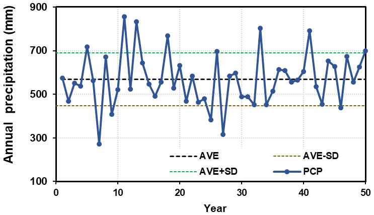
Figure 4 Time series of annual precipitation (mm). The dashed coloured lines represent the average values (AVE) and ±1 standard deviation (SD).

2.2.3 Soil and water

The soil properties were investigated by sampling over a profile 5.0 m below the ground at the study site. The dry bulk density (ρ_b, g cm⁻³) was obtained by drying volumetric soil samples (100 cm³) at 105 ^∘C for 48 h, and the soil particle size distribution and organic matter content were measured in the laboratory. Silt loam dominated the profile, with moderate variations among the soil layers. On average, the silt loam consisted of 5.8 % sand, 73.4 % silt, and 20.9 % clay (Ma et al., 2017).

The saturated hydraulic conductivity (K_s, cm h⁻¹) was measured in the undisturbed soil samples using a constant-head method (Ramos et al., 2017). The field capacity (θ_fc) and wilting point (θ_wp) were derived from the power function (Campbell, 1974; Clapp and Hornberger, 1978), corresponding to the soil potentials of −33 and −1500 kPa respectively.

Volumetric soil moisture sensors were installed in 14 layers within a depth of 500 cm from the surface: at 5, 15, 30, 45, 60, 90, 120, 150, 200, 250, 300, 350, 400, and 500 cm respectively (Fig. 3). The sensors, CS-655 soil water content reflectometers (Campbell Scientific, Inc., Logan, UT, USA), have been in operation since June 2014. A CR1000 data logger (Campbell Scientific, Inc., Logan, UT, USA) records the data every 10 min.

The soil properties below 5.0 m were adopted from previous studies (Li et al., 2008; Jia et al., 2017a; Wu et al., 2021) on black locust plantations in the Loess Plateau.

The soil desiccation index (SDI) was used to evaluate the degree of soil desiccation for the comparison between the observation and simulation results; this index was calculated as follows:

$$\begin{array}{}\text{(20)}& \mathrm{SDI}={\displaystyle \frac{\mathit{\theta }-{\mathit{\theta }}_{\mathrm{wp}}}{{\mathit{\theta }}_{\mathrm{sfc}}-{\mathit{\theta }}_{\mathrm{wp}}}},\end{array}$$

where θ_sfc is the soil water content at a stable field capacity. In practice, a soil water content at 60 % of field capacity (θ_fc) can be assumed to be the stable field capacity of loess in the Loess Plateau (Wang et al., 2011). Soil layers with an SDI < 1 were regarded as drying soil layers.

2.2.4 Plants

The leaf area index (LAI, m² m⁻²) of the black locust canopy was measured using an optical method (Jonckheere et al., 2004), biweekly or triweekly during the growing seasons of 2014, 2015, and 2016. An 8 mm fisheye lens (Sigma F3.5 EX DG circular fisheye, Sigma Corporation) mounted on a Canon EOS 5D digital SLR camera (http://www.canon.com, last access: 20 December 2020) took hemispherical photographs of the canopy on cloudy days. The photographs were analysed using the CAN_EYE software to derive the LAI values (Demarez et al., 2008). Within each plot, photographs were taken at five different positions each time. The LAI value for the plot is the average of the five positions.

The measured LAI values were compared to those of the Moderate Resolution Imaging Spectroradiometer (MODIS) MYD15A2H product, which has a spatial resolution of 500 m and a temporal resolution of 8 d. Furthermore, the 8 d MODIS LAI series were downscaled to a daily series using the Savitzky–Golay filtering technique (Tie et al., 2017).

The root profiles were investigated in August 2015. A 150 cm wide trench, which was located between two neighbouring rows and perpendicular to the row direction, was excavated 500 cm below the ground (Fig. 3). During the excavation, soil samples, 20 cm in the horizontal dimension and 40 cm in vertical thickness, were taken along the trench and over the profile. It is assumed that the roots develop homogeneously along the horizontal row but unevenly along the trench. Finally, seven samples were collected from each soil layer across the trench. The soil samples were rinsed, and the weight and length of fine roots (less than 2 mm in diameter) were measured for each sample.

To estimate the parameters of the black locust root system, a pot experiment was carried out in 2016 (planted in April and sampled in October), the details of which are given in Fig. S1 in the Supplement.

In addition to the measurements mentioned above, data on black locust roots, including the density profile and rooting depth were compiled from the published literature (see Supplement).

2.3 Model set-up

2.3.1 Initial and boundary conditions for the Richards' equation

In solving the Richards' equation numerically, the vertical domain extends from the surface to 20 m below the ground. The domain was discretized into adjoining layers with a thickness of 5 cm each.

The upper boundary condition was set as the flux of the rainfall rate with the canopy interception removed or the soil evaporation rate. As the soil water content in deep soil (20–100 m) is relatively stable around the field capacity (Qiao et al., 2018), the lower boundary was set to a constant soil water content at the field capacity.

During the calibration and validation stages, the initial soil water profile was determined using the measurements. The initial soil water profile was set at the field capacity when the model was applied to the long-term simulation.

2.3.2 Numerical simulations

The soil hydraulic parameters, saturated hydraulic conductivity K_s and constant B in the soil water retention curve, were initialized by the measured values. They were further tuned to match the simulated soil water content to the observations.

The vegetation growth parameters were adapted from Zhang et al. (2015), who simulated the black locust growth in the Loess Plateau using the Biome-BGC model. Other vegetation parameters were obtained from the SWAT model (Neitsch et al., 2011; Sun et al., 2011).

All the relevant parameters are summarized in Table S1 in the Supplement.

2.3.3 Numerical simulations

The numerical simulations consist of two parts, the short-term (5 years) simulation for model calibration and validation, and the long-term simulation (50 years) for investigation:

1. The model calibration and validation were performed for the observation period (2014–2018). The model was calibrated from 1 June 2014 to 31 December 2016 and validated through 1 January 2017 to 31 December 2018. The measured LAI, soil water content, and root profiles were used for the evaluation. The rooting depth was assumed to be 5.0 m below the ground for three approaches, considering the relatively short period of the field experiment.

2. A long-term simulation was performed to explore the forest root–soil water interactions over a period of 50 years, with the aim of investigating the drying soil layer evolution over the long term considering inter-annual variation in precipitation. The long-term simulation adopted the data from Yongshou Station for 1971–2020 without any sense of a specific historical period. In the long-term simulation, a value of 5.0 m was set for the rooting depth of the static approaches; an initial value of 50 cm was set for the dynamic rooting depth approach. Plants start to grow at the beginning of the simulation.

2.3.4 Evaluation indices

Statistical indices, the coefficient of determination (R²), the Nash–Sutcliffe efficiency (NSE), and the percent bias (PBIAS), were used to evaluate model performance and are given as follows:

$$\begin{array}{}\text{(21)}& {\displaystyle }& {\displaystyle }{R}^{\mathrm{2}}={\displaystyle \frac{\sum _{i=\mathrm{1}}^n\left(S_i-\stackrel{\mathrm{‾}}{S}\right)\left(O_i-\stackrel{\mathrm{‾}}{O}\right)}{\sqrt{\sum _{i=\mathrm{1}}^n\left(S_i-\stackrel{\mathrm{‾}}{S}\right)\sum _{i=\mathrm{1}}^n\left(O_i-\stackrel{\mathrm{‾}}{O}\right)}}};\text{(22)}& {\displaystyle }& {\displaystyle }\mathrm{NSE}=\mathrm{1}-{\displaystyle \frac{\sum _{i=\mathrm{1}}^n{\left(O_i-S_i\right)}^{\mathrm{2}}}{\sum _{i=\mathrm{1}}^n{\left(O_i-\stackrel{\mathrm{‾}}{O}\right)}^{\mathrm{2}}}};\end{array}$$

$$\begin{array}{}\text{(23)}& \mathrm{PBIAS}={\displaystyle \frac{\sum _{i=\mathrm{1}}^n\left(S_i-O_i\right)}{\sum _{i=\mathrm{1}}^n{O}_i}}\times \mathrm{100}\mathit{\%}.\end{array}$$

Here, S_i is the simulated value at time step i, $\stackrel{\mathrm{‾}}{S}$ is the mean of the simulated value, O_i is the observed value at time step i, $\stackrel{\mathrm{‾}}{O}$ is the mean of the observed value, and n is the number of time steps. R² and NSE were dimensionless. The dimension of the PBIAS was percent (%).

R² describes the proportion of the variance in the measured data explained by the model, ranging from 0 to 1, with higher values indicating less error variance. The NSE indicates the consistency between the plot of the observed vs. simulated data and the 1:1 line, ranging between −∞ and 1.0 (1 inclusive) and optimized at the value of 1. The PBIAS measures the average tendency of the simulated data to be larger or smaller than the observation, and a lower value implies a more accurate model simulation, with optimization at 0.0. Positive values indicate a model underestimation bias, and negative values indicate a model overestimation bias. Moriasi et al. (2007) proposed a widely used rating system, which judged the modelling performance as “very good”, “good”, “satisfactory”, or “unsatisfactory” using PBIAS < ±10 %, ±10 % ≤ PBIAS < ±15 %, ±15 % ≤ PBIAS < ±25 %, or PBIAS ≥ ±25 % respectively or using 0.75 < NSE ≤ 1.0, 0.65 < NSE ≤ 0.75, 0, 0.50 < NSE ≤ 0.65, or NSE ≤ 0.50 respectively.

3 Results

3.1 Model calibration and validation

The model parameters, maximum LAI (LAI_max), saturated hydraulic conductivities (K_s), and exponent of the soil–water characteristic curve (B), were calibrated and validated using the field measurements. The initial value of the LAI_max was assigned a default of 5.0 in the SWAT model; the initial values for K_s and B were based on measurements in the laboratory of the samples taken from the field site. The soil hydraulic parameters varied for the different soil layers. The calibration was performed manually using the observed LAI and soil water content as the target. The performance was evaluated using the indices mentioned in the previous section, and the calibrated values are listed in Table S1.

The simulated LAI values were plotted against the field measurements for 2014–2016 for calibration and 2017–2018 for validation (Fig. 5). Further, the MODIS-derived LAI values were used for evaluating the simulation over the entire period as well, especially for the validation period of 2017–2018, for which the field measurements were not available.

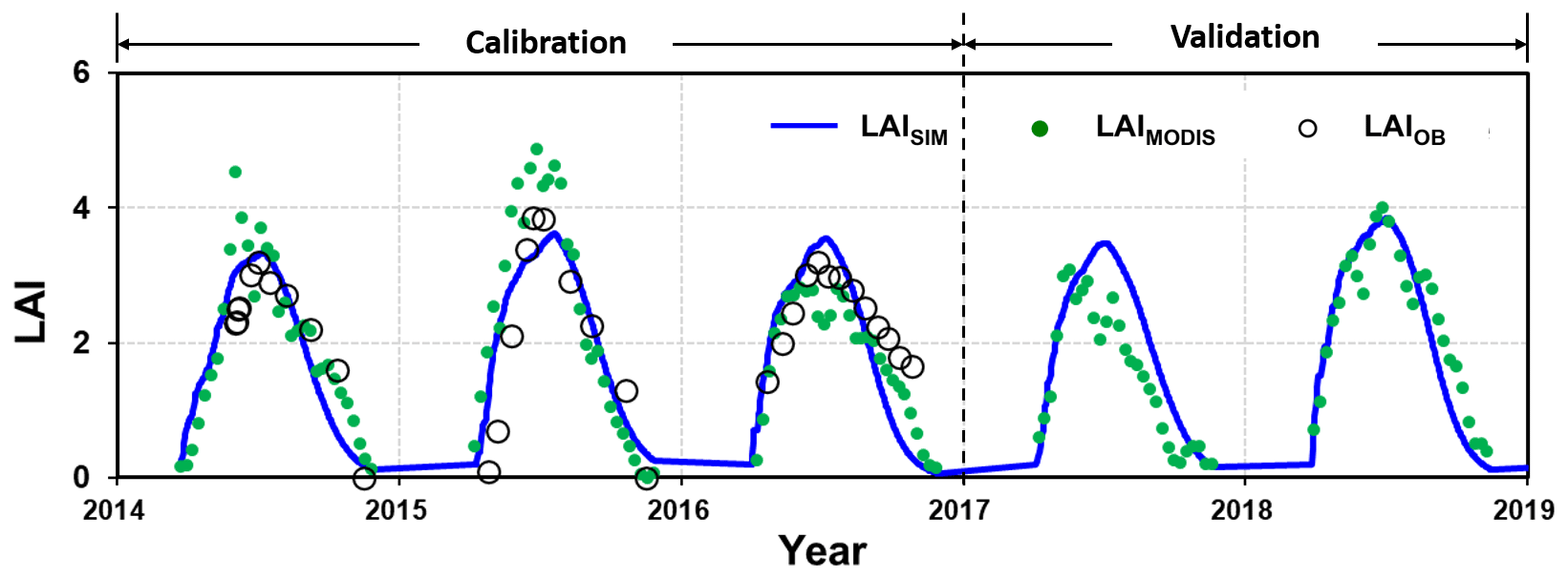
Figure 5 Comparison of the leaf area index (LAI) from simulation (LAI_SIM), MODIS-derived data (LAI_MODIS), and plot observation (LAI_OB) for the calibration (2014–2016) and validation (2017–2018) periods.

During the calibration period, the simulated LAI values fit the measurements with a classification of “very good” (Moriasi et al., 2007), with an NSE of 0.60 and a PBIAS of 5.2 %. Validation with the MODIS-derived LAI indicated a “very good” performance (Moriasi et al., 2007), with an NSE of 0.80 and a PBIAS of 17.5 %.

The MODIS-derived LAI exhibited remarkably similar seasonal patterns to the field measurements. Over- or underestimation was also noticed, for example, in 2014–2016 and 2017 respectively (Fig. 5). Other studies have reported that overestimation may specifically occur for the LAI during the wet season when compared with the field experiments (Yang et al., 2006; Naithani et al., 2013) or when cross-evaluated against other remote-sensing-based products (Garrigues et al., 2008). The simulation demonstrated an overestimation of the LAI when compared with the MODIS-derived LAI in 2017. Although it is also argued that the MODIS-derived LAI may underestimate reality (Fang et al., 2012), it is not sure which one (or both) is responsible for the discrepancy between the simulated and observed values in 2017 due to the unavailability of field measurements. The point-pixel comparison issue might also be a reason for the quantitative difference between the MODIS-derived and field-measured LAI. Nevertheless, the evaluation indices indicate the acceptance of the LAI_max by the model performance in both the calibration and validation stages.

Figure 6 shows a simplified comparison of the average soil water content (SWC) over the 5.0 m profile, which illustrates the differences among the root growth simulations. The simulations reproduced the patterns in the SWC throughout the seasons and between rainfall events exceptionally well in both the calibration and validation stages. The dynamic fine-root distribution approaches (S–D and D–D, which refer to the static rooting depth and dynamic fine-root distribution approach and the dynamic rooting depth and dynamic distribution of fine-roots approach respectively) reproduced the variations in SWC remarkably well; however, the static rooting depth and static fine-root distribution (S–S) approach deviated significantly. Therefore, the results of this approach will no longer be discussed in the following sections.

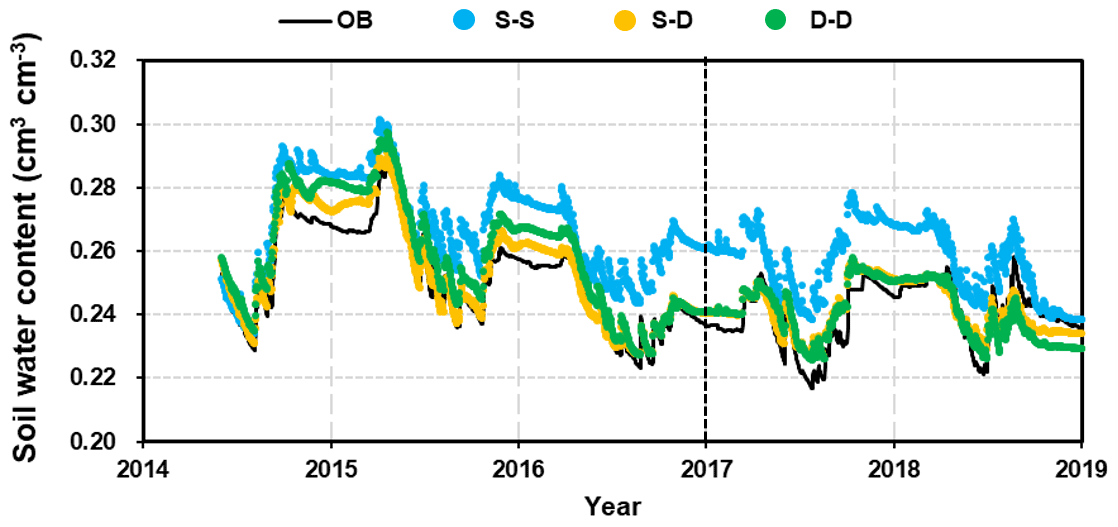
Figure 6 Comparison of the 5 m profile-averaged soil water content (SWC) from observations (OB) and the three root simulation approaches during the calibration (2014–2016) and validation (2017–2018) periods. The abbreviations used in the figure are as follows: S–S – static rooting depth and static fine-root distribution; S–D – static rooting depth and dynamic fine-root distribution; D–D – dynamic rooting depth and dynamic distribution of fine roots.

The evaluation indices R² values for the static and dynamic rooting depth approaches were 0.96 and 0.96, the NSE values were 0.91 and 0.71, and PBIAS values were 1.2 % and 2.9 % respectively at the calibration stage; at the validation stage, the R² values were 0.66 and 0.64, the NSE values were 0.66 and 0.58, and the PBIAS values were 7.0 % and 0.4 % respectively. This model performance can be categorized as “good” or “very good” following the rating system by Moriasi et al. (2007).

The fine-root density profiles produced during the calibration and validation stages were compared with the sampled values obtained in August 2015 (Fig. 7). The measured fine-root densities varied significantly among the seven sampled profiles, and the variations decreased with soil depth. The simulated fine-root densities exhibited an even wider range of variations, which covered the growth seasons from 2014 to 2018. On average, the root distribution of the dynamic rooting depth approach was closer to the measurements than that of the static rooting depth approach.

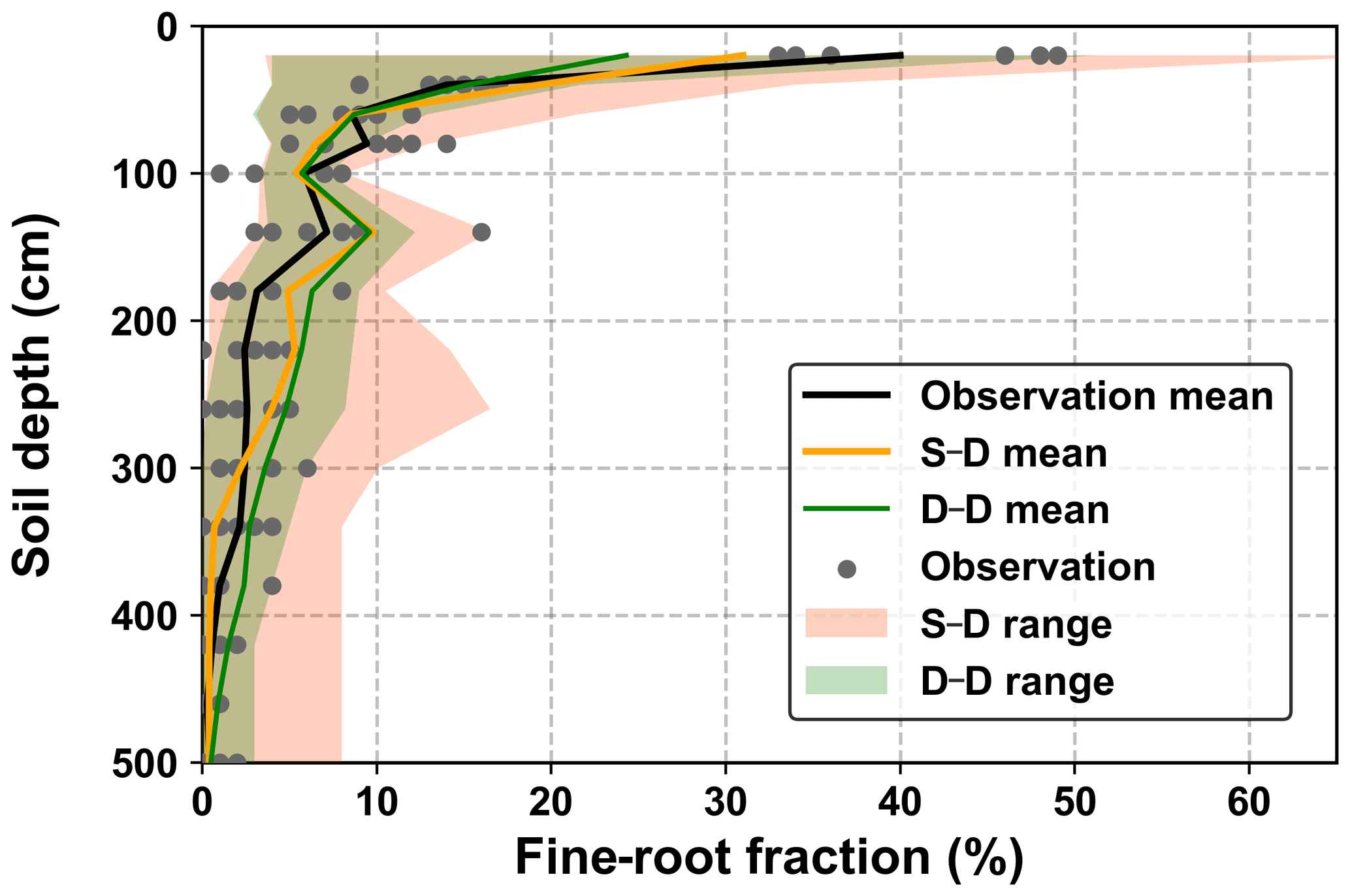
Figure 7 Comparison of the 5 m profile-averaged soil water content (SWC) from observations (OB) and the two root simulation approaches during the calibration (2014–2016) and validation (2017–2018) periods. The abbreviations used in the figure are as follows: S–D – static rooting depth and dynamic fine-root distribution; D–D – dynamic rooting depth and dynamic distribution of fine roots.

Variations in fine-root distribution simulated by the static and dynamic rooting depth resulted from strategies for simulating the root–soil water interactions. In the static rooting depth approach, the growth of fine roots was purely determined by soil water availability and its distribution within the rooting domain, for example, 5.0 m in this study (see Eqs. 3 and 5 in Sect. 2.1.4). In contrast, in the dynamic rooting depth approach, growth of the fine roots may demand an increment of coarse roots that will cost more carbon and is finally determined by the optimization of the cost–benefit functions, as described by Eqs. (12) and (18). Thus, the dynamic root depth approach resulted in a narrower variation range than the static rooting depth approach. Averaged over the simulation period, the dynamic rooting depth approach achieved a more homogeneous fine-root distribution profile than the static rooting depth approach, implying that the former approach utilized more soil water from the deeper soil layers. This point will be further addressed in the discussion regarding the drying soil layer evolution over the long term.

3.2 Long-term simulation

3.2.1 Rooting depth and soil water

Simulations forced by the long-term climatic data series revealed root development using the static and dynamic rooting depth approaches (Fig. 8a). Instead of assigning a fixed root depth of 5.0 m in the static rooting depth approach, the dynamic rooting depth approach simulated the root depth extension, which is consistent with the data from the literature. It was found that the rooting depth may be as deep as 11.0 m below the ground. The simulated rooting depth extension rate slowed as the stand age increased, which was also consistent with the observations in artificial forests (see in Fig. S4; Christina et al., 2011; Wang et al., 2015). Furthermore, the simulated root profiles by the two approaches within a 2.0 m soil depth were also evaluated against the data collected from the literature (Fig. 8b, c). The simulated results varied within the range provided by the data in the literature. Regressions between the mean fine-root fractions by the static and dynamic rooting depth approaches and that of the literature data provided R² values of 0.34 and 0.64 respectively, indicating that the dynamic approach performed better than the static approach.

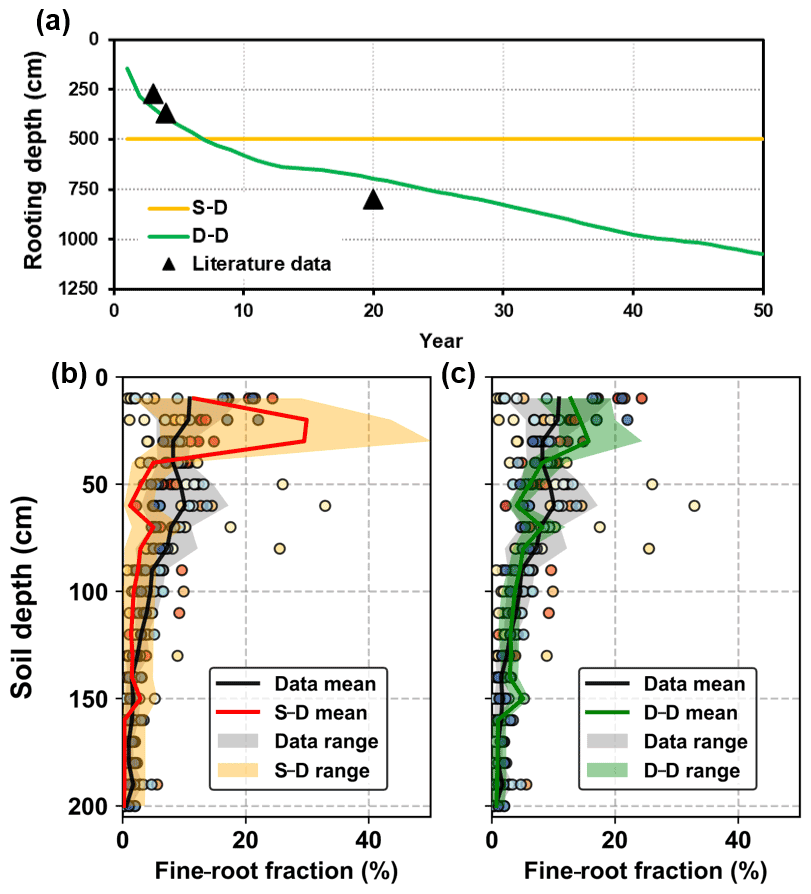
Figure 8 Evaluation of the simulated root distribution against the literature data: (a) rooting depth, (b) fine-root distribution in the top 2.0 m soil layer for the static rooting depth approach (S–D), and (c) fine-root distribution in the top 2.0 m soil layer for the dynamic rooting depth approach (D–D). The scatters with different colours illustrate the observational data from different literature sources, and the shaded areas illustrate the range of the mean ± standard deviation of simulation.

The evolution of root growth and soil water over the long term is depicted in Fig. 9. Visually, wetting and drying processes over the soil profiles were commonly found from simulations of both root growth modelling approaches. However, the difference in the simulated soil water distribution was also significant (Fig. 9d).

Figure 9 Time series of (a) monthly precipitation (mm per month), (b) soil water content (SWC) along the 20 m soil profile simulated by the static rooting depth (S–D) approach, (c) soil water content along the 20 m soil profile simulated by the dynamic rooting depth (D–D) approach, and (d) the difference in the SWC between the S–D and D–D approaches. The dashed black horizontal line in panel (b) and the curve in panel (c) indicate the rooting depth.

These two approaches resulted in substantially different spatial distributions of roots and soil water and, thus, a significant difference in root–water interactions. The soil water varied significantly with precipitation during the entire period. In most years, the maximum infiltration depth was less than 2.0 m. Meanwhile, precipitation could infiltrate down to 5.0 m in consecutive wet years, for example, the period from the 10th to 15th years. Notably, a time lag effect existed between the peak precipitation and the maximum infiltration depth: the peak precipitation occurred around August, while the maximum infiltration depth was reached around March in the following year.

3.2.2 Infiltration

Precipitation replenishes soil water through infiltration. The amount and depth of the infiltrated water impact the growth and water use of the root systems. The infiltration is associated with the a priori soil water content and its distribution over the profile, the amount and duration of an individual precipitation event, and the effects of the randomly sequential events. Establishing a relationship between the infiltration depth and precipitation on the basis of a single event is complicated and difficult to achieve. Instead, analyses were performed on an annual basis; that is, the maximum infiltration depth vs. the annual precipitation amount were regressed for the two root growth modelling approaches, as shown in Fig. 10. During the simulation period of 50 years, the annual precipitation varied from 250 to 850 mm. It was found that the annual infiltration amounts from these two approaches were exceptionally close to each other. The dynamic rooting depth approach was 4.0 % lower than that of the static rooting depth approach, which is an insignificant difference, as discussed in a later section. The maximum infiltration depth was positively correlated with the annual precipitation, which is not uncommon. The results also indicated that the maximum infiltration depth may reach 6.0 m below the ground in very wet years. Interestingly, the regression lines of these two root growth modelling approaches crossed at approximately 500 mm of annual precipitation. When annual precipitation was less than 500 mm, the infiltration reached deeper soil for the static rooting depth approach, and the inverse was found when the annual precipitation was more than 500 mm.

Figure 10 Comparisons of (a) infiltration amounts and (b) maximum infiltration depths between the static rooting depth (S–D) and dynamic rooting depth (D–D) approaches.

3.2.3 Fine-root distribution and water uptake

The fine-root distributions simulated by these two approaches showed exceptionally similar patterns in the soil profile (Fig. 11a). However, a quantitative difference between them was also noticeable. For the static rooting depth approach, roots grow only within the soil layer with a present 5.0 m thickness. For the dynamic rooting depth approach, the coarse roots reach 11.0 m below the ground. Within the top 2.0 m soil layer, the fractions of fine roots for the static and dynamic rooting depth approaches were 90.0 % and 80.3 % respectively, and within the 2.0–5.0 m soil layer, these values were 10.0 % and 14.7 % respectively. For the dynamic rooting depth approach, only 5.0 % of fine roots were in the soil below 5.0 m.

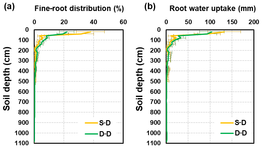
Figure 11 Profile of (a) fine-root density distributions (%) and (b) root water uptake distributions (mm) resulting from different approaches (the S–D and D–D approaches). The error bars represent the standard error (SE) of the mean of different years.

The distribution of root water uptake over the soil profile was similar to that of the fine-root density (Fig. 11b). The static rooting depth approach resulted in an annual water uptake of 338 mm (SD = 84 mm), whereas the dynamic rooting depth approached 381 mm (SD = 84 mm). In the top 2.0 m soil layer, the root uptake was 298 and 318 mm for the static and dynamic rooting depth approaches respectively. In the 2.0–5.0 m layer, the values for the static and dynamic rooting depth approaches were 40 and 40 mm respectively. Below 5.0 m, the dynamic approach resulted in a root uptake of 24 mm, which accounted for 6.2 % of the uptake from the entire profile.

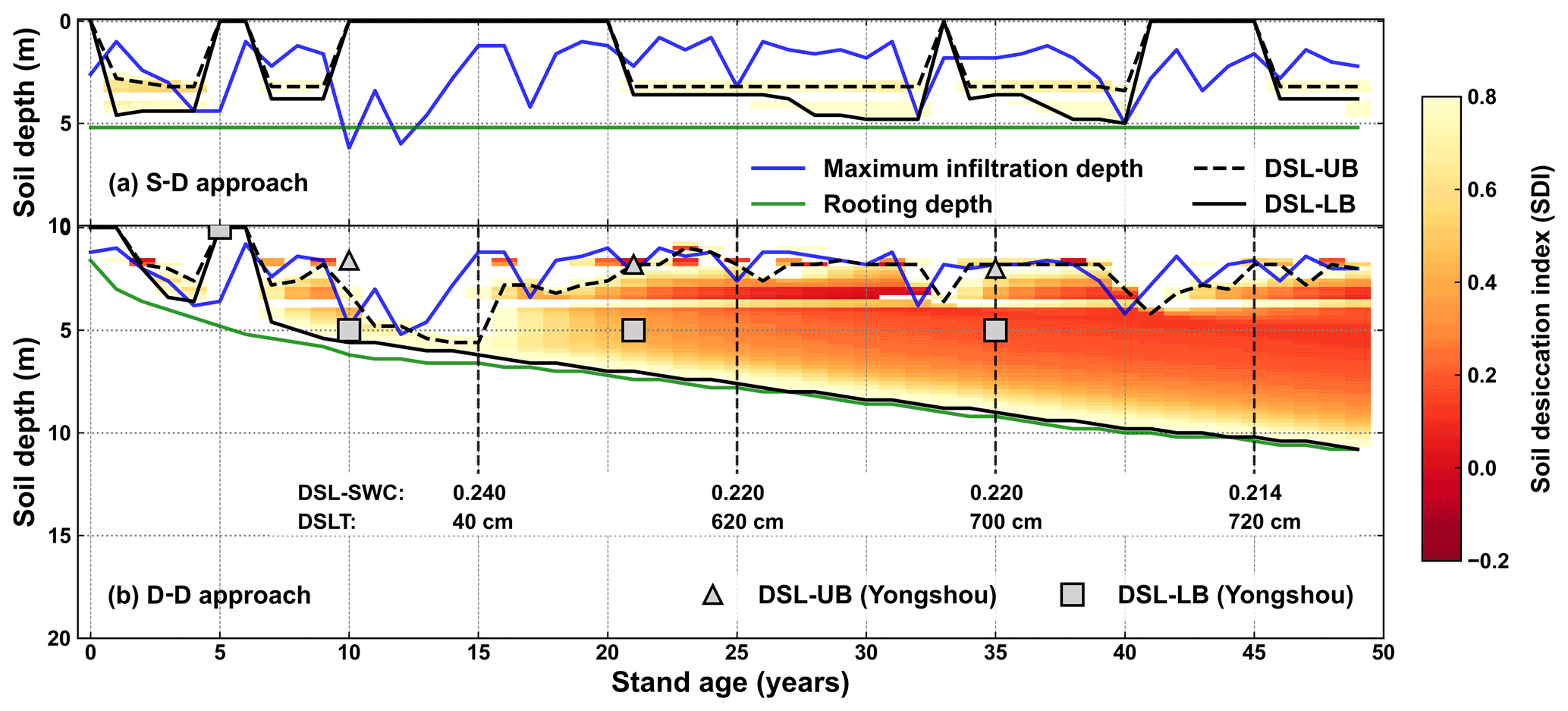
Figure 12 Evolution of the drying soil layers with stand age simulated by (a) the static rooting depth (S–D) and (b) the dynamic rooting depth (D–D) approaches over a 50-year period at Yongshou, Loess Plateau. The triangles and squares are the respective observed upper and lower boundaries adopted from Jia et al. (2017a). The abbreviations used in the figure are as follows: DSL-UB – the upper boundary of the drying soil layer; DSL-LB – the lower boundary of the drying soil layer; DSL-SWC – the mean soil water content within the drying soil layer; DSLT – the thickness of the drying soil layer.

3.2.4 Evolution of drying soil layers

The long-term soil water evolution is illustrated in Fig. 9. Vertically, the most active soil water zone was within the top 2.0 m (statistically based on the simulation results). This was confirmed by root development and water uptake in this study (Fig. 11) and by field observations in this region (Suo et al., 2020). In the top 2.0 m soil layer, infiltration events replenish and plant roots deplete the soil water alternately. The two root growth modelling approaches resulted in remarkably similar soil water enrichment and depletion patterns in the top 2.0 m layer, especially during the infiltration period (Fig. 9d). Below the top 2.0 m, soil water was continuously in a negative state, and the dynamic rooting depth approach resulted in more soil water depletion than the static rooting depth approach.

Drying soil layers have been frequently reported in previous studies in the Loess Plateau (Y. Wang et al., 2018). The upper and lower boundaries of the drying soil layers were defined according to the soil desiccation index (Wang et al., 2011), as shown in Fig. 12. The static rooting depth approach did not demonstrate the sustainable existence of drying soil layers. This is because it pre-sets a fixed rooting depth over the simulation period, which does not capture the hydraulic traits of roots that may develop to use water from the wetter zone beneath the pre-set rooting depth.

For the dynamic rooting depth approach, the drying soil layers started to develop at a stand age of approximately 8 years and became deeper and thicker sustainably with increasing stand age. Its lower boundary extended gradually to deeper soil, while its upper boundary fluctuated significantly. The strong fluctuations were associated with the infiltration, whereas the continuous extension of the lower boundary was due to sustained plant root uptake and rare recharge. With stand ageing, the soil water content in the drying soil layer decreased continuously, and the thickness increased gradually.

The simulated evolution of the drying soil layers was partially confirmed by field observations (Jia et al., 2017a), as shown in Fig. 12. The simulation produced a progressive course of the lower boundary, which was far deeper below the ground than the observations. The observations were limited to the top 5.0 m only. A deeper sampling might have resulted in a thicker drying soil. In Changwu, which is 80 km from the study site in the Loess Plateau, it was reported that the thickness of the drying soil layer reached 7.0 m, with its lower boundary as deep as 8.0 m below the ground in the black locust plantation (Li et al., 2008). It should also be noted that the sampling depth was limited to 8.0 m. Deep sampling has indicated that drying soil layers reach a depth of 19.0 m in the Loess Plateau (Wu et al., 2021).

4 Discussion

4.1 Root–water interactions and drying soil layers

As indicated in Sect. 1, this study attempted to develop a root growth model that can simulate coarse-root extension dynamically instead of the static rooting depth approach currently adopted in most available models (Sivandran and Bras, 2013; Wang et al., 2016; P. Wang et al., 2018; Drewniak, 2019; Niu et al., 2020). In formulating the dynamic rooting depth, the study proposed a cost–benefit algorithm based on ecophysiological principles (Chen et al., 2019). The evaluation of the simulated results against the field observations from this study and from the literature proved its effectiveness for the Loess Plateau.

The static rooting depth approach is widely used in ecological and hydrological models, which have been employed to simulate soil water variations in field crops, shrubs, and forests in the Loess Plateau (Zhang et al., 2015; Tian et al., 2017; B. Li et al., 2019; Bai et al., 2020). Short-term model calibration and validation, ranging from months to 5 years, have usually shown acceptable performance, whereas long-term evaluation has rarely been undertaken. When used to address the long-term issue in this study, comparisons between the static and dynamic rooting depth approaches indicated that the former did not reproduce the occurrence and evolution of the drying soil layers due to its pre-set rooting depth (Fig. 12). The drying soil layers simulated by the static approach were discontinuous along the soil profile (Fig. S5), due to sufficient precipitation infiltration recharging the soil moisture during the humid period. Meanwhile, the lower boundary of the drying soil layers was less than 5.0 m, which was constrained by the fixed tree rooting depth. These results are inconsistent with the actual conditions observed by deep sampling in this region, which indicated a deeper, continuous drying soil layer (Wang et al., 2013; Zhao et al., 2019). Therefore, the static rooting depth approach reflected neither the change in soil moisture in the deeper layer (>5.0 m) nor the evolution of the drying soil layers, as it did not allow for the deeper water uptake by roots.

Notably, the development of drying soil layers is predominantly due to water utilization by the deep fine roots, which accounts for only approximately 5 % of the total profile uptake (Fig. 11). Although minor compared with the total, it caused a sustained negative soil water balance in the deep soil due to difficulties in receiving recharge, as described in the results section. The continuous development of the lower boundary of the drying soil layer implies that its recovery is critically difficult. This is because of the large thickness and vast storage capacity of loess soil (Huang and Shao, 2019). Plants tend to develop more fine roots in the topsoil and use more soil water due to lower costs but higher benefits, resulting in a more profitable adaptation strategy when experiencing water stress. Exploration of water from wetter but deeper soil is also an adaption strategy when it is more profitable, but deep roots might be more expensive to construct and maintain (Pierret et al., 2016; Germon et al., 2020). This explains why the top 2.0 m soil was the most active zone of water uptake in this study. Depletion of topsoil always vacates the storage for infiltration, making it difficult for the rainfall to replenish the deeper dried soil layer or groundwater (Turkeltaub et al., 2018).

The occurrence and development of a drying soil layer significantly impact the plant–water relationship and the local hydrological cycling in the Loess Plateau, where the combination of deep loess soil and the semi-arid and arid climate prevails (Zhao et al., 2019). This might also be an issue in other regions with similar soil and climate conditions (Shao et al., 2018); in fact, this phenomenon has also been reported elsewhere, such as in the Amazonia forest (Jipp et al., 1998) and southern Australia dryland (Robinson et al., 2006), due to artificial afforestation. The occurrence of a persistent drying soil layer not only degrades soil and vegetation but also negatively impacts ecosystem functions and services (Huang and Shao, 2019), such as the degeneration of the artificially planted trees (Jia et al., 2017a). The drying soil layer and the degraded artificial afforestation are believed to be mutually causative. The long-term simulation results also affirm the importance of monitoring both the long-term vegetation and soil water dynamics of artificial forests for ecosystem restoration practices in the Loess Plateau, for example, the “Grain for Green” project implemented in 1999.

4.2 Outlooks of future work

Roots develop beneath the ground, which is widely accepted to be critically difficult to monitor; the deeper the soil depth, the harder it is to sample (Maeght et al., 2013; Warren et al., 2015; Fan et al., 2017). Observations of the rooting depths are rarely available for ready use, especially knowledge of the maximum rooting depth for vegetation in a region. Occasionally, the limited data may provide a rough estimate; for example, H. Li et al. (2019) and Wu et al. (2021) reported some maximum rooting depths of apple trees and black locust of approximately 25.0 m (H. Li et al., 2019; Wu et al., 2021). Mathematical simulation is a beneficial compensation for field observations and can go far beyond its limitations, although its effectiveness relies on the actual data. The simulation can reproduce the dynamics of roots at very fine temporal and spatial resolutions, while in situ data are usually extremely rare. This study adopted in situ data at only a single moment, as shown in Fig. 3. Fortunately, it was found that the measurements fell within the variation range of the simulations over some time periods, which is understandable from a statistical point of view. In situ data are believed to remain an issue in the development and evaluation of root approaches in the long term (Pierret et al., 2016).

The simulation results indicated that the annual infiltration amount from the static rooting depth approach was 4.0 % higher than that of the dynamic rooting depth approach (Fig. 10). In the field, no surface runoff was found during the years of observation at the study site at Yeheshan. The minor difference in the infiltration amount between these two rooting depth approaches was due to canopy interception. The static rooting depth approach limits the roots to develop and use water within the top 5.0 m soil layer, whereas the dynamic rooting depth approach permits the root to grow into deep wetter soil for uptake, which can release more soil water stress. The lower the soil water stress, the greater the leaf area and canopy storage. This small difference in the infiltration amount between these two approaches highlights the internal relationship between the above- and below-ground parts of the plants. The allocation of biomass between the above- and below-ground parts changes with climate, soil water, and nutrients over time and varies among vegetation types (Poorter et al., 2012; Qi et al., 2019). These mechanisms were involved in the model of this study. However, this study adopted a fixed allocation factor in order to focus on investigating the temporal and spatial changes in the rooting depth, fine-root distribution, and their impacts on soil water evolution over the long term. Further attempts will be made to investigate the systematic behaviour of the plants with respect to their adaptation strategies in order to obtain the maximum cost–benefit ratio by optimizing the biomass allocation between the above- and below-ground parts via a trade-off strategy (Trugman et al., 2019; Sakschewski et al., 2021) and the spatial distribution of roots over the soil profile.

5 Summary

Root–soil water interaction is currently a frontier topic, and several publications have reported the recent progress in root uptake modelling approaches. The key issue involved is the root growth modelling approach, simulating the spatial distribution of fine and coarse roots over the soil profile. The modelling approaches of rooting depth, for example variable rooting depth that is empirically formulated as a function of tree height in the humid Amazon region where soil water is usually not a limiting factor of tree growth (Sakschewski et al., 2021), are one of the most recent achievements in this field. We developed an approach for simulating variable rooting depth coupled with soil water dynamics and optimized by a cost–benefit function in a semi-arid and arid climate region where plants experience soil water stress. An evaluation of the different types of root uptake models against field data indicated that the new approach does not stand out among the previous models during a short period of time. However, long-term application to the drying soil layer in the Loess Plateau indicated that incorporating dynamic rooting depth into the currently available root growth model is a necessary step for attaining an in-depth understanding of the occurrence and evolution of the widely reported drying soil layer phenomenon in this region.

The long-term simulations of the evolution of a drying soil layer indicated that the top 2.0 m of the soil layer is always the most active zone of soil water variation and root uptake. The percentages of fine roots and water uptake below the 2.0 m soil layer account for only 5.0 % and 6.2 % of the total over the soil profile respectively. However, although these are relatively small, they cause a persistently negative water balance and a consequent drying soil layer. The rooting depth increases to utilize deeper soil water when soil water stress occurs in the upper soil layer, driving the lower boundary of the drying soil layer downward. As the upper 2.0 m soil layer intercepts most of the infiltration of rainfall events, replenishment of the deeper soil by infiltration is very unlikely. Continuous thickening of the drying soil layer and the associated difficulties in recovery may have strong implications for forest–water management in this region as well as in other regions with similar climates and soils.