the Creative Commons Attribution 4.0 License.
the Creative Commons Attribution 4.0 License.
 | 16 Mar 2022
Combining passive and active distributed temperature sensing measurements to locate and quantify groundwater discharge variability into a headwater stream
Olivier Bour
Mikaël Faucheux
Nicolas Lavenant
Hugo Le Lay
Ophélie Fovet
Zahra Thomas
Laurent Longuevergne
Exchanges between groundwater and surface water play a key role for ecosystem preservation, especially in headwater catchments where groundwater discharge into streams highly contributes to streamflow generation and maintenance. Despite several decades of research, investigating the spatial variability in groundwater discharge into streams still remains challenging mainly because groundwater/surface water interactions are controlled by multi-scale processes. In this context, we evaluated the potential of using FO-DTS (fibre optic distributed temperature sensing) technology to locate and quantify groundwater discharge at a high resolution. To do so, we propose to combine, for the first time, long-term passive DTS measurements and active DTS measurements by deploying FO cables in the streambed sediments of a first- and second-order stream in gaining conditions. The passive DTS experiment provided 8 months of monitoring of streambed temperature fluctuations along more than 530 m of cable, while the active DTS experiment, performed during a few days, allowed a detailed and accurate investigation of groundwater discharge variability over a 60 m length heated section. Long-term passive DTS measurements turn out to be an efficient method to detect and locate groundwater discharge along several hundreds of metres. The continuous 8 months of monitoring allowed the highlighting of changes in the groundwater discharge dynamic in response to the hydrological dynamic of the headwater catchment. However, the quantification of fluxes with this approach remains limited given the high uncertainties on estimates, due to uncertainties on thermal properties and boundary conditions. On the contrary, active DTS measurements, which have seldom been performed in streambed sediments and never applied to quantify water fluxes, allow for the estimation of the spatial distribution of both thermal conductivities and the groundwater fluxes at high resolution all along the 60 m heated section of the FO cable. The method allows for the description of the variability in streambed properties at an unprecedented scale and reveals the variability in groundwater inflows at small scales. In the end, this study shows the potential and the interest of the complementary use of passive and active DTS experiments to quantify groundwater discharge at different spatial and temporal scales. Thus, results show that groundwater discharges are mainly concentrated in the upstream part of the watershed, where steepest slopes are observed, confirming the importance of the topography in the stream generation in headwater catchments. However, through the high spatial resolution of measurements, it was also possible to highlight the presence of local and highly contributive groundwater inflows, probably driven by local heterogeneities. The possibility to quantify groundwater discharge at a high spatial resolution through active DTS offers promising perspectives for the characterization of distributed responses times but also for studying biogeochemical hotspots and hot moments.
- Article
(5822 KB) - Full-text XML
-
Supplement
(1679 KB) - BibTeX
- EndNote


Understanding groundwater and stream water interactions as integral components of a stream catchment continuum is crucial for the efficient development and management of water resources (Bencala, 1993; Brunke and Gonser, 1997; Sophocleous, 2002). Particularly essential for the preservation of groundwater-dependent ecosystems and riparian habitats (Kalbus et al., 2006), these interactions play a major role in physical, geochemical, and biological processes occurring in the stream or in the hyporheic zone (Frei et al., 2019; Jones and Mulholland, 2000). More specifically, these exchanges control water quality affecting river ecohydrology and hydrochemistry, particularly during dry periods when groundwater is the principal contribution to stream discharge (Brunke and Gonser, 1997). This is particularly true in headwater catchments, where groundwater discharge highly contributes to streamflow generation (Winter, 2007). However, localizing and quantifying exchanges between groundwater and stream water is often difficult, as these exchange are controlled by multi-scale processes and are, therefore, highly variable in time and in space (Brunke and Gonser, 1997; Fleckenstein et al., 2006; Flipo et al., 2014; Harvey and Bencala, 1993; Kalbus et al., 2009; Varli and Yilmaz, 2018; Woessner, 2000).
A wide range of methods exists to estimate water fluxes between stream- and groundwater, including solute tracer concentrations (Brandt et al., 2017; Liao et al., 2021), seepage meter measurements (Rosenberry et al., 2020), or the use of heat as a groundwater tracer (Anderson, 2005; Constantz, 2008), which is particularly efficient in identifying patterns of focused discharge. The approach relies on the detection of temperature anomalies observed at the sediment–water interface (Tyler et al., 2009; Sebok et al., 2013; Westhoff et al., 2011) or into the streambed (Krause et al., 2012; Lowry et al., 2007) when significant differences exist between groundwater and stream water temperatures. Then, the comparison of temperature variations monitored at different depths in the streambed provides information on groundwater discharge (Anderson, 2005; Constantz, 2008; Hatch et al., 2006; Keery et al., 2007; Lapham, 1989; Stallman, 1965; Webb et al., 2008; Winter et al., 1998). Indeed, the diurnal or seasonal water temperature variations propagate deeper for losing streams (downward conditions) than for gaining streams (upward conditions), since heat transfer is either attenuated or enhanced by groundwater discharge (Constantz, 2008; Goto et al., 2005). Thus, the use of vertical thermal profiles (VTPs) is widely applied for determining flow directions, quantifying groundwater discharge (Hatch et al., 2006; Lapham, 1989; Keery et al., 2007) and estimating hydraulic parameters (Constantz and Thomas, 1996). Nevertheless, only point measurements of the stream–aquifer interactions are achievable with this approach. Considering the spatial variability and the complexity of flow at the groundwater (GW)/stream water interface, extensive information on spatial and temporal temperature patterns are required to gain a more complete understanding of flows at reach scale and even more at watershed scale.
This was made possible by the development and the use of the fibre optic distributed temperature sensing (FO-DTS) technology for environmental applications (Selker et al., 2006a, b; Shanafield et al., 2018; Tyler et al., 2009). FO-DTS provides continuous temperature data through space and time along fibre optic cables at a high spatial resolution (Habel et al., 2009; SEAFOM, 2010; Ukil et al., 2012). By deploying FO cables at the bottom of the stream, the DTS technology allows temperature monitoring of the longitudinal linear stream/sediments interface, allowing the detection of thermal anomalies induced by groundwater discharge into the stream (Briggs et al., 2012; Gilmore et al., 2019; Koruk et al., 2020; Moridnejad et al., 2020; Rosenberry et al., 2016; Selker et al., 2006a, b; Westhoff et al., 2007, 2011). This approach was also used to study seasonal and temporal fluctuations in groundwater discharge into streams (Matheswaran et al., 2014; Slater et al., 2010) and into a lake (Sebok et al., 2013). Energy balance models have been efficiently applied to interpret passive DTS measurements and quantify GW/stream water exchanges (Selker et al., 2006b; Westhoff et al., 2011). However, their use remains limited because it requires monitoring significant temperature changes over time, limiting the application of the method to large groundwater inflows or small headwater streams. To overcome such limitations, some studies proposed to detect thermal anomalies in the streambed by burying the FO cable into the streambed sediments in the hyporheic zone (Krause et al., 2012; Le Lay et al., 2019b; Lowry et al., 2007) to improve the possibility of localizing GW inflows.
Despite that, the quantification of fluxes from passive DTS measurements remains challenging. In theory, the implementation of three FO cables buried at different depths, as proposed by Mamer and Lowry (2013), would be ideal to measure the attenuation of the stream temperature variations into the sediments in order to obtain high-resolution fluxes estimates. Unfortunately, such an approach is technically very difficult to apply in the field. Considering this difficulty, Le Lay et al. (2019a) proposed coupling FO-DTS data collected along a single fibre optic cable at a given depth with point temperature measurements from thermal lances. In the approach, it is assumed that temperature boundary conditions can be characterized from the temperature measurements collected with the thermal lances and extrapolated all along the stream to be combined with FO-DTS measured at a given depth. Moreover, the question of sediments thermal properties and their spatial variability remained unexplored, even though thermal conductivity highly impacts flux estimates (Sebok and Müller, 2019). Based on these assumptions, they showed the temporal variability in exchanges associated to the annual hydrological cycle and the possibility of estimating diffuse groundwater inflows (Le Lay et al., 2019a).
Alternatively, active DTS methods, consisting of heating the FO cable, have been recently developed to improve the capabilities of FO-DTS methods for estimating fluxes in different environmental conditions (Bense et al., 2016; Simon et al., 2021a). In particular, it was demonstrated that the difference in temperature between an electrically heated and a non-heated FO cable is directly dependent on water fluxes, offering the possibility to estimate fluxes (Bense et al., 2016; Read et al., 2014; Sayde et al., 2015). Thus, active DTS methods have been used to estimate wind speed in the low atmosphere (Lapo et al., 2020; Sayde et al., 2015; van Ramshorst et al., 2020), in dam monitoring (Ghafoori et al., 2020; Perzlmaier et al., 2004; Su et al., 2017), for groundwater fluxes measurements in open (Banks et al., 2014; Klepikova et al., 2018; Read et al., 2014, 2015) and sealed boreholes (Munn et al., 2020; Selker and Selker, 2018) or else in direct contact within sedimentary aquifers (del Val et al., 2021; des Tombe et al., 2019). Despite promising developments, active DTS methods have seldom been used in hydrology to estimate groundwater/surface water interactions. Kurth et al. (2015) coupled passive and active DTS measurements and highlighted areas with lower and higher flow rates over the cable, but the quantification of fluxes remained unexplored. Briggs et al. (2016) developed a novel probe to quantify vertical fluxes at a high resolution using active DTS measurements, but the probe only permits a local-scale characterization of the stream–aquifer dynamic.
In this study, we propose to use, for the first time, active DTS measurements to quantify groundwater discharge in the stream of a headwater catchment. The application of active DTS methods in such a context is particularly promising since the interpretation of active DTS measurements in saturated porous media provides estimates of both sediments thermal conductivities and groundwater fluxes over a large range and with an excellent accuracy (Simon et al., 2021a). This method should allow the quantifying of groundwater discharge and characterizing of the streambed thermal properties at an unprecedented spatial scale. To complement active DTS measurements, which were limited in space and time, an 8-month passive DTS experiment was conducted at the catchment scale in order to infer the temporal and spatial patterns of groundwater discharges over the investigated period. Therefore, this study also investigates how these two experiments could be compared and combined to characterize both the spatial and the temporal dynamics of groundwater discharge. To do so, FO cables were deployed in the streambed sediments of a headwater stream within a small agricultural watershed. In the following, we first present the headwater catchment and the experimental set-up before presenting the methods used to interpret both passive and active DTS measurements. Fluxes estimates obtained with both passive and active DTS measurements are then compared, and the advantages and limitations of each method are finally discussed.
2.1 The experimental set-up on the Kerrien watershed
2.1.1 The Kerrien watershed
The experiment has been conducted in the Kerrien watershed located in southwestern Brittany (4∘7′24.87′′ W, 47∘56′26.97′′ N). It is part of the AgrHys Environmental Research Observatory, whose principal aim is to understand and characterize transit times in small agricultural catchments (ORE AgrHys, 2021). The site is a part of the French network of critical zone observatories (Gaillardet et al., 2018) and supports extensive hydrological and geochemical research. This site was selected because it presents the advantage of readily installed equipment and instruments (Fovet et al., 2018).
As shown in Fig. 1, the watershed is a headwater watershed with a second-order stream, subdivided into three first-order sub-watersheds, namely the Kerrien, the Kerbernez, and the Gerveur sub-watersheds. The Kerrien sub-watershed is a small agricultural watershed (9.5 ha), with steeper slopes in the upper parts (14 % slopes) than in the bottom lands (5 % slopes), characterized by a large wetland (Ruiz et al., 2002). As pointed out in Fig. 1, downstream the wetland, the fields were converted into a golf course. In this artificial environment, the stream has been completely restored and dammed to facilitate maintenance. Drainage pipes contribute to drain precipitation from the watershed area directly into the stream, limiting the potential groundwater recharge by draining precipitation from the watershed area into the stream. Further downstream, the stream reaches a natural wood plain.
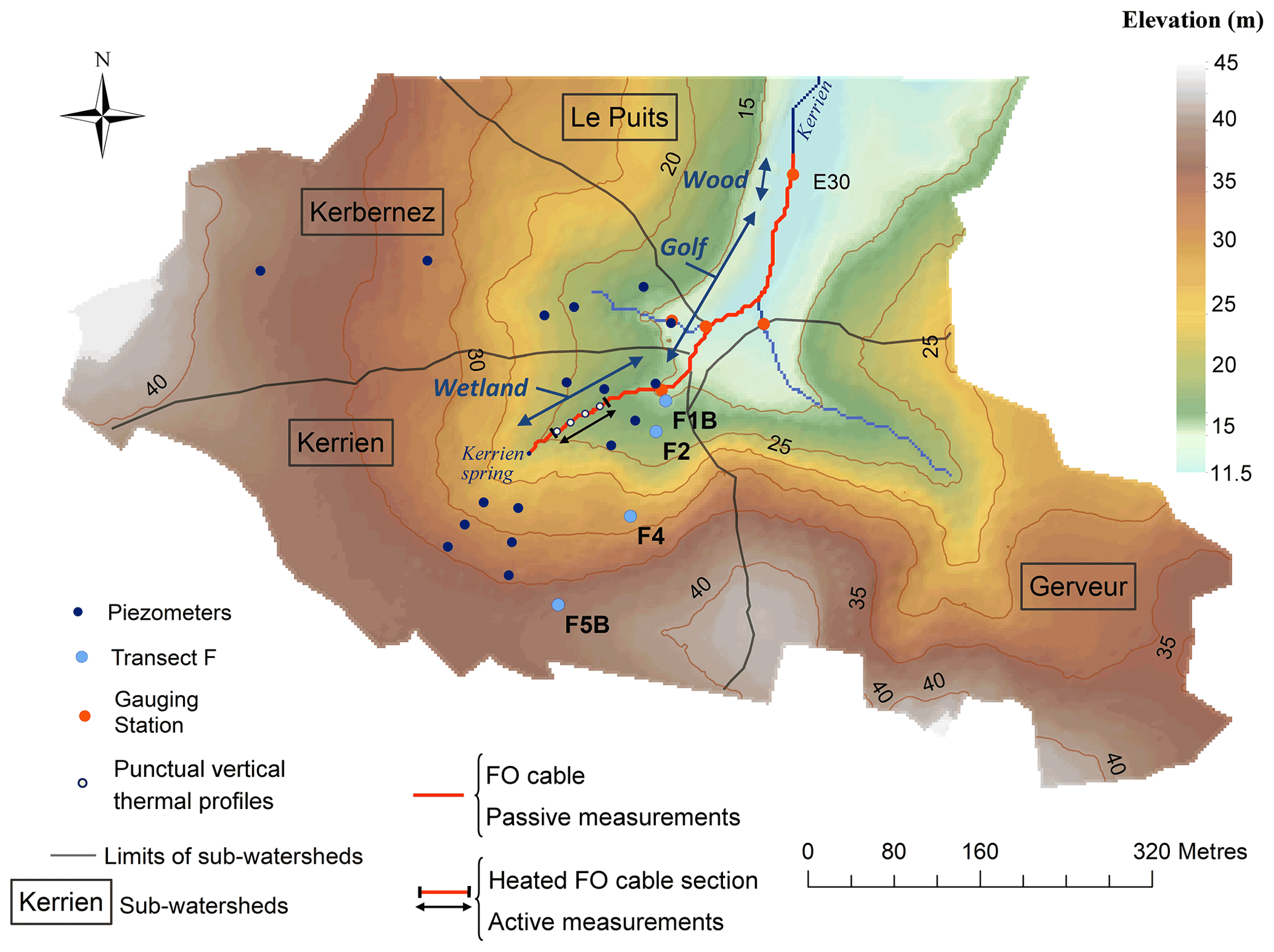
Figure 1Description of the watershed with the location of piezometers, gauging station, and fibre optic cables.
2.1.2 Hydrological dynamics of the study site
The Kerrien watershed has been particularly studied and instrumented for estimating transit times in a small agricultural watershed (Fovet et al., 2015a; Martin, 2003), as shown in Fig. 1. For this study, we are using the data from the piezometer transfect F (Fig. 1), including the hillslope piezometer F5b (20 m depth) and the mid-slope piezometer F4 (15 m depth), as markers for the deep groundwater storage dynamics, and the riparian piezometers F2 (2 m depth) and F1b (5 m depth), as markers for the riparian groundwater storage dynamics. The gauging station E30 provides stream flow rate.
Runoff is insignificant, so that most of the effective precipitation is infiltrating in this headwater watershed. The annual rainfall (1114 mm on average) is well distributed over the year, but recharge mainly occurs in autumn and winter. Therefore, the contribution of groundwater to the stream flow reaches 80 %–90 % (Fovet et al., 2015b; Martin et al., 2006; Ruiz et al., 2002), with the stream discharge during high water periods being highly correlated with hillslope head gradient (Martin, 2003). As shown in Fig. 2a, piezometric levels show clear seasonal fluctuations with high levels during winter and spring and low levels during summer and autumn. The hydraulic gradient between the aquifer and the stream, as well as the evolution of the stream discharge, suggests that groundwater discharge into the stream should be particularly expected during the high water level period (from December to June).
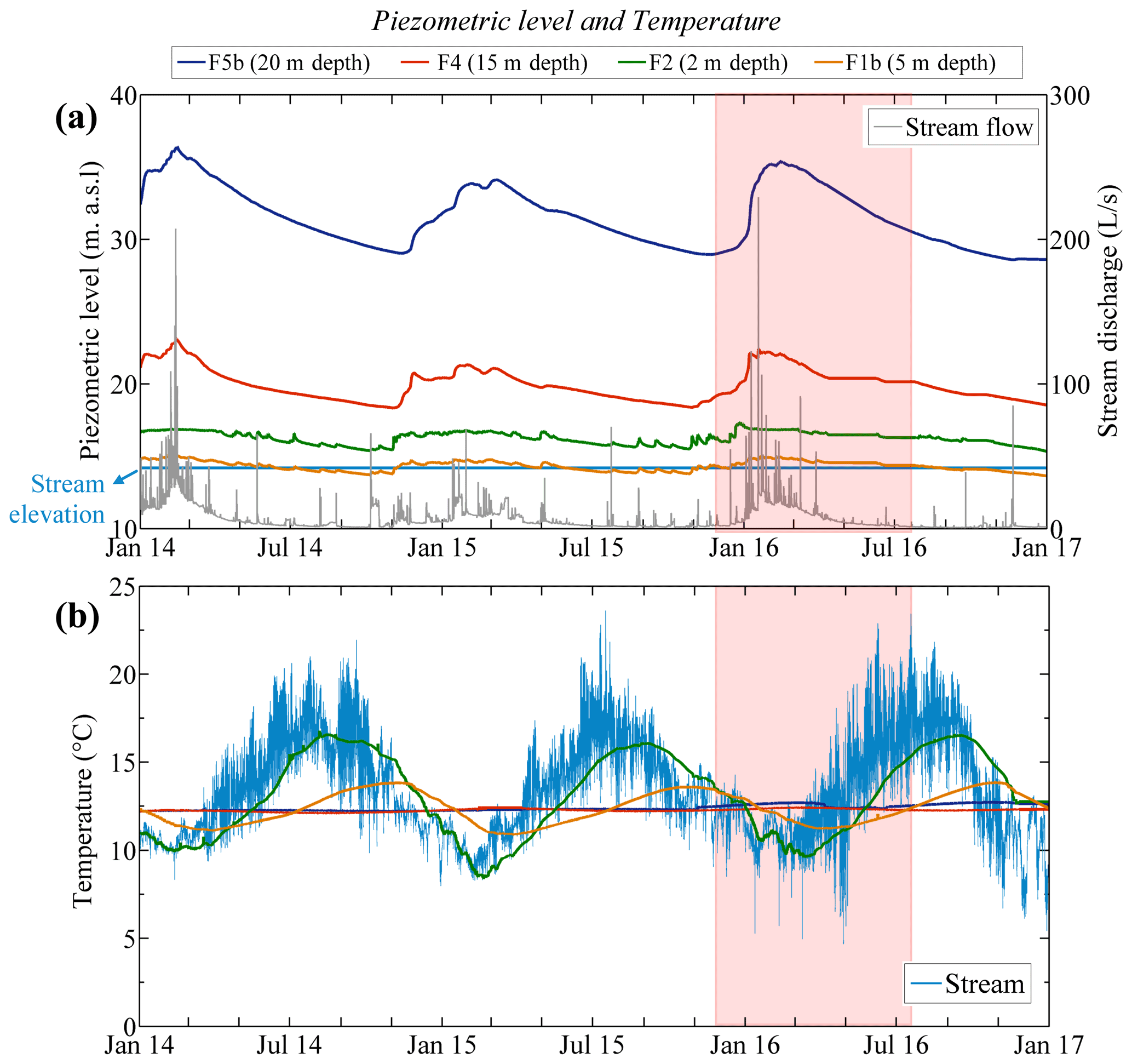
Figure 2(a) Changes in stream flow and in piezometric levels along the transect F over 3 years. (b) Stream- and groundwater temperature fluctuations over time along the transect F. The red-coloured area corresponds to the period of passive DTS measurements conducted from December 2015 to 15 July 2016.
Figure 2b shows temperature fluctuations in the stream and in piezometers over a time period from July 2013 to May 2017. While the groundwater temperature is almost constant in the upslope domain (piezometers F5b and F4), temperature variations recorded in the stream and in the downslope domain (F2 and F1b) show larger variations following daily and seasonal temperature variations. It can easily be shown that temperature variations recorded in F2 and F1b result from the diffusion of air temperature variations through the water columns of piezometers. The detection in the stream of thermal anomalies induced by groundwater discharge requires a significant contrast of temperature between stream and groundwater, as well as a significant groundwater discharge compared to the stream flow. Here, considering the relatively small difference in temperature between groundwater and stream water and in order to detect potential diffusive inflows, the choice was made to bury the FO cable within the sediments, which should facilitate the detection of potential temperature anomalies as marker of groundwater discharge (Krause et al., 2012; Le Lay et al., 2019b; Lowry et al., 2007). Otherwise, active DTS measurements should highlight advective heat transfer controlled by groundwater discharge.
2.2 Passive DTS measurements and data interpretation
2.2.1 FO cable deployment and data acquisition
To investigate the temporal and spatial dynamics of groundwater discharge, a FO cable has been deployed in the streambed sediments in the southern part of the study site, as shown in Fig. 1. Streambed temperature variations were recorded along this cable using the DTS technology from December 2015 to July 2016. The FO cable has been deployed downstream from the Kerrien spring. In total, more than 530 m of a BruSens FO cable have been buried directly into the streambed. Due to some obstacles (coarse gravels, cobbles, gauging stations, etc.), it was not possible to bury the FO cable in few places. Everywhere else, the average burial depth was estimated to be 8 cm. The first 165 m of the FO cable have been deployed in the Kerrien sub-watershed, where the stream is surrounded by a wetland. The streambed is formed by sand and sludge, whose thickness is low but large enough to bury the cable properly. Then, besides a harder substrate, the FO cable was deployed in the golf course area. In few local places, the burying was not possible, and the FO cable was set on the streambed. The last 70 m of the FO cable have been deployed in a wood plain, a natural environment, where a deeper sandy riverbed facilitates cable burying. As highlighted in Fig. 2a, the 8-month experiment ensured the monitoring of streambed temperature during both high and low water tables. The highest levels were recorded from January to mid-April, the period over which the wetland is saturated up to the surface.
The FO cable has been connected to a FO-DTS control unit, a Silixa XT-DTS instrument (5 km range). The DTS unit was configured in a double-ended configuration (van de Giesen et al., 2012) to collect data at 25 cm and 10 min sampling interval. The use of two calibration baths (one at the ambient temperature and a fridge) and PT100 probes (0.1 ∘C) and RBRsolo T probes (0.002 ∘C accuracy) allowed for the calibration of the data. To assess the accuracy of temperature measurements, a RBRsolo T probe was set up at the gauging station E30 located at the entrance of the wood. A comparison between DTS measurements and RBRsolo T probes validated the temperature measurements, with a relative uncertainty of measurements (standard error) estimated at 0.05 ∘C and an absolute uncertainty of measurement that can reach, at maximum, 0.2 ∘C, depending on the period of measurement.
In complement, four vertical temperature profiles (VTPs) were installed in the streambed in the wetland area by deploying temperature sensors (HOBO U12-015-02 sensors – ±0.25 ∘C precision) at 12.5 and 22 cm depth in the streambed sediments. The position of these sensors in the stream is shown in Fig. 1 and was chosen at locations where groundwater discharge has been observed using preliminary results obtained from FO-DTS monitoring. From upstream to downstream, the VTPs are numbered from 1 to 4. For each location, the evolution of temperature was recorded from 7 April 2016 to 3 May 2017. These VTPs will be used to quantify local groundwater discharge, and the results will be compared with estimates from FO-DTS measurements.
2.2.2 Data interpretation
Groundwater inflows can be detected by localizing temperature anomalies. Those can be easily identified by plotting the evolution of the temperature over time and space, especially for a long time series. Thermal anomalies can also be identified using an analysis of the standard deviation (SD) of temperature for a given period (Sebok et al., 2015), since the calculation of the standard deviation provides insights about amplitudes of temperature variations. In case of groundwater discharge, the value of the SD of streambed temperature is expected to be much lower than the value of the SD of the stream temperature. Therefore, relative variations in fluxes along the cable could be determined from relative variations of SD.
Then, to quantify vertical fluxes, we use the FLUX-BOT model, a code proposed by Munz and Schmidt (2017), using a numerical heat transport model to solve the 1D heat transport equation (Carslaw and Jaeger, 1959; Domenico and Schwartz, 1998). This 1D model allows the calculation of the specific discharge in the z direction (i.e. the vertical Darcy flux) by inverting the measured time series observed at least at three different depths. Temperature variations are simulated according to the optimized fluxes. The quality criteria calculated between the simulated temperatures and the measured one (Nash–Sutcliffe efficiency, NSE, R2, and root mean square error, RMSE) allow the discussion of the quality of flux estimates. Thus, the model estimates the direction and the intensity of the flow and may highlight the temporal variability in exchanges.
To apply the model, the stream temperature and the groundwater temperature were chosen as upper and lower boundary conditions, respectively. The stream temperature was measured for the wetland area at the Kerrien spring with a temperature sensor and at the gauging station E30 (RBRsolo T) for the wood plain area. The temperature signal recorded at 15 m depth in the piezometer F4 (Fig. 2b) was used to set the groundwater temperature. The FLUX-BOT model was first used for interpreting the temperature measurements of the four VTPs installed in the streambed. Considering the upper and lower boundary conditions previously defined, the numerical model reproduces the temperature evolution collected at 12.5 and 22 cm depth and provides an estimate of vertical fluxes for each profile. Details about the interpretation of VTPs using the FLUX-BOT model are provided in the Supplement (Figs. S1 and S2). The results are compared in Sect. 3.3, with estimated fluxes from passive and active DTS measurements. Identically, the FLUX-BOT model is used to reproduce and interpret passive DTS measurements collected at various spots along the cable. A loop was added in the initial code, allowing the interpretation of data collected for each measurement point. For both applications, the vertical mesh size of the model was set at 0.01 m, as recommended by Munz and Schmidt (2017). Concerning the thermal properties of the saturated sediments, the volumetric heat capacity was set at 3×10⁶ J m−3 K−1. The streambed sediments being composed of saturated clay, silt, sand, and gravel, the thermal conductivity may typically range between 0.9 and 4 W m−1 K−1 (Stauffer et al., 2013). Thus, considering the importance of the sediment thermal conductivity on groundwater fluxes estimates (Sebok and Müller, 2019), the model was applied for three values of thermal conductivity (1, 2.5, and 4 W m−1 K−1).
2.3 Active DTS measurements
Active DTS measurements were conducted in April 2016, concurrently with passive DTS measurements, by deploying an additional FO cable within the streambed in the wetland, as shown in Fig. 1. While the active DTS experiment was conducted, passive DTS measurements had already been collected for 3 months, which allowed the highlighting of clear and significant temperature anomalies along the cable deployed in the wetland area (see Sect. 3). Assuming that these temperature anomalies could be associated to potential groundwater exfiltration zones, the choice was made to conduct the active DTS experiment in this area.
Figure 3 presents the experimental set-up of the active experiment. A FO cable is electrically heated through its steel armouring, and the elevation in temperature, associated to the heat injection, is continuously monitored all along the heated section using the FO inside the cable. Without any flow, heat transfers occur through the porous media only by conduction and a gradual and continuous increase of temperature is therefore expected (Simon et al., 2021a). If water flows through the porous medium, advection partly controls the thermal response by dissipating a part of the heat produced by the heat source. The higher the water flow, the lower the temperature increase should be (Simon et al., 2021a). Contrary to passive DTS measurements, one of a main advantage of the method is the possibility of investigating groundwater fluxes in any conditions, independently of natural temperature gradients. However, similarly to most thermal-based methods (Constantz, 2008), it is assumed that groundwater flows are perpendicular to FO cables (Simon et al., 2021a).
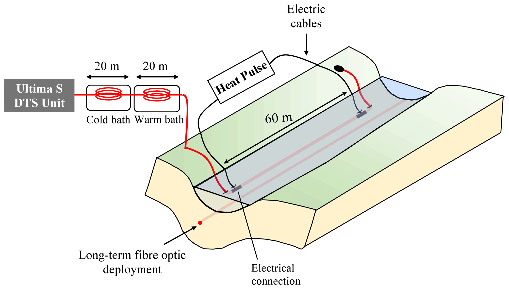
Figure 3Experimental set-up of the active experiment. A 60 m section of a heatable cable has been electrically isolated, buried in the sediments, and then heated by connecting to a power controller.
For the active DTS experiment, 150 m of a BruSens FO cable have been connected to a FO-DTS control unit, a Silixa ULTIMA S instrument. The unit was configured in double-ended configuration to collect data at 12.5 cm sampling and 60 s time interval. The effective spatial resolution of DTS measurements with this unit was estimated, varying between 66 and 90 cm, following the methodology proposed in Simon et al. (2020). The calibration process applied was almost similar to the one applied for calibrating passive DTS measurements. The only difference is that a warm calibration bath was used as reference section during the active DTS experiment, while a bath at ambient temperature was used for the passive DTS experiment. To do so, heating resistors were set in the bath, and air pumps were used to homogenize the temperature within. Considering the important temperature rise expected during the active experiment, using a warmed calibration bath is essential because the bath temperatures must preferably bracket the full range of temperatures expected to occur along the cable (van de Giesen et al., 2012).
Note that, while passive DTS measurements have been monitored all along the stream, a much shorter section of FO cable has been used for the active DTS experiment, due to the power limitations (3300 W) of the generator used for power supply. A 60 m section of the 150 m FO cable has been buried in the streambed in parallel with the FO cable previously installed for the passive experiment. As the heating experiment induces a very localized thermal perturbation within the streambed, the non-heated cable was not affected by the heat injection. Thus, natural streambed temperature fluctuations were monitored during the experiment using the non-heated cable. It should be noted that, during the FO cable deployment in the streambed, local heterogeneities led to the impossibility of deploying the whole FO heating section in the streambed. Thanks to cable numbering, these non-buried sections were accurately located. For buried sections, the burial depth was measured in situ and estimated to be around 8 to 10 cm. This 60 m section has been electrically isolated and heated using a power controller (provided by CTEMP; DTS and Accessory Systems, 2021) supplying a constant and uniform heating rate power of 35 W m−1 along the heated FO cable. The heated cable was energized continuously during 4 h, and the recovery was also monitored for an additional 3 h after turning off the power controller.
Before interpreting the data, data were processed to remove the measurement points corresponding to sections where the cable was not buried in the streambed but laid at the bottom of the stream. These sections were precisely marked during the cable installation. Moreover, since the temperature increase is mainly controlled by convection in the stream, thermal responses measured during the heating phase in the non-buried sections of the cable are different from thermal responses observed in buried section and are easily identifiable with temperature rises reaching steady-state in 1 or 2 min (Read et al., 2014). Then, the data processing method developed in Simon et al. (2020), which consists of calculating the derivative of the temperature with respect to distance, was applied. It allows highlighting areas where the temperature changes occur at a scale smaller than the spatial resolution of measurements, which leads to identifying measurements that are representative of the effective temperature.
Finally, among all the section used for active DTS measurements, 172 measurements points are thought to be significant. Note that the raw data of active DTS measurements, the data processing (sorting and quality check), and the definition of significant points are presented in detail in the Supplement. The data were further interpreted using the ADTS toolbox, proposed by Simon and Bour (2022), for automatically interpreting active DTS measurements. The ADTS toolbox contains several MATLAB codes that allow the estimation of the thermal conductivities and the groundwater fluxes (specific discharge) and their respective spatial distribution all along the heated section. The method is based on an analytical approach proposed and validated by Simon et al. (2021a), which consists of defining, for each measurement point along the heated section, the optimized values of thermal conductivity and flux that allow the reproduction of, at best, the associated temperature increase measured over the heating period. The use of the ADTS toolbox also provides an estimate of the associated uncertainties (Simon and Bour, 2022).
In the following, we first focus on the interpretation of passive DTS measurements with the aim of locating groundwater discharges and characterizing the temporal dynamics. Then, we present and analyse the results of the active DTS experiment, which are performed during a few days. Both results are further compared.
3.1 Passive DTS measurements
3.1.1 Spatial variability of temperature signals
Figure 4a synthesizes the results of the passive DTS experiment and shows temperature signals monitored all along the FO cable deployed in the streambed sediments. The x axis indicates the distance between the Kerrien spring (located at 0 m) and each measurement point in the streambed. Temperature variations are presented from December 2015 to July 2016 (y axis). In June and July, despite very low flows, the stream never dried up. There are two different behaviours highlighted in the figure. On the one hand, vertical yellow lines can be observed near the Kerrien spring in the first 150 m of the cable. These lines emphasize that the temperature recorded in these areas is relatively constant over time (few temperature variations are recorded). On the other hand, away from the spring, beyond 300 m, clear and large differences in temperature are observed between colder periods (from December to mid-April) and warmer periods (from mid-April to July).
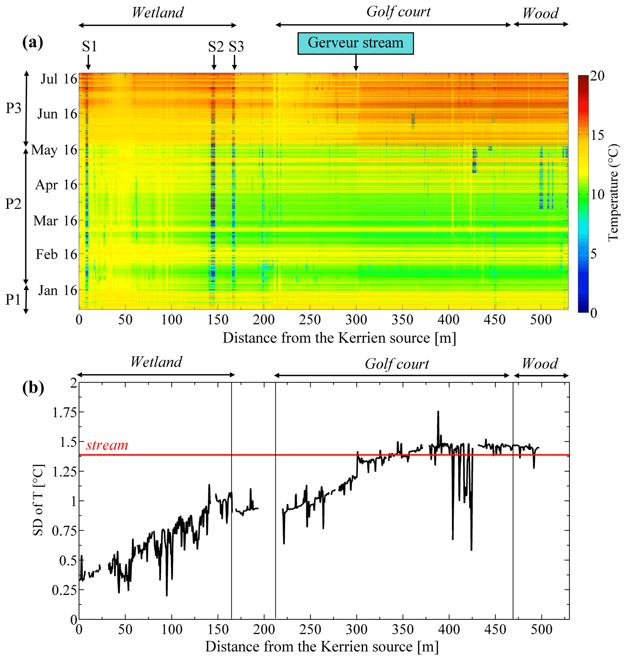
Figure 4(a) Long-term monitoring of streambed temperature along the river using DTS. Sections S1, S2, and S3 match with spots where the cable lies on the bank because of obstacles in the stream (gauging stations). Temporary thermal anomalies located, for instance, in 425 m and around 500 m correspond to air-exposed periods during which the cable was not held at the sediment/water interface. (b) Standard deviation (SD) of the temperature calculated over the experiment duration for each measurement point along the FO cable. Sections where the cable was outside the stream or punctually unburied were removed. The red line represents the SD of the stream temperature (1.38 ∘C) measured at the gauging station E30.
To highlight the spatial variability in the temperature signal, the standard deviation (SD) in the temperature was calculated for each measurement point over the whole duration of the experiment, as presented in Fig. 4b. The value of the SD of stream temperature (≈ 1.375 ∘C) directly reflects the amplitude of daily temperature fluctuations. Concerning the SD of streambed temperature, its value is relatively stable and very low (around 0.37 ∘C) in the first 50 m of measurements near the spring. Then, it progressively increases from upstream to downstream and stabilizes around the value of the SD of the stream temperature at around 300 m (in the middle of the golf course area).
The lowest SD values are recorded in the upstream wetland (d < 160 m in Fig. 4b). In this area, as illustrated in Fig. 5a by the red curve (94.56 m, σ= 0.2 ∘C), the temperature is relatively stable over time (around 12.5 ∘C), and the daily stream temperature fluctuations are widely attenuated (the SD varies between 0.19 and 0.93 ∘C, while the SD of the stream temperature is 1.38 ∘C). However, significant differences are observed between temperature measurements from upstream to downstream, as highlighted by the progressive increase in SD measured from the spring to 160 m. This increase reflects the increase in the amplitudes of daily temperature fluctuations collected from upstream (orange line in Fig. 5b; σ= 0.36 ∘C) to downstream (grey line in Fig. 5b; σ= 0.95 ∘C). In addition, the profile of SD (Fig. 4b) also shows isolated spikes associated with very low SD values, which is in agreement with the yellow lines observed in Fig. 4a. These spikes can be associated with spots where the amplitude of temperature is low all over the period of measurements, as illustrated by blue curve in Fig. 5b (53.38 m), where the value of the SD is equal to 0.24 ∘C. As we shall see in the next few sections, the relative temperature stability suggests that these spikes or hotspots may be associated with local groundwater discharges.
Further downstream (from 220 up to 300 m in the first part of the golf course area), while the value of the SD progressively increases (Fig. 4b), higher amplitudes of daily temperature variations are monitored, as illustrated in the Fig. 5a by the blue curve (227.5 m, σ= 0.93 ∘C). In this area, SD values are lower than the one calculated in the stream (1.3 ∘C; Fig. 4b), meaning that the daily temperature fluctuations are slightly attenuated. Once again, the progressive increase in the value of the SD highlights differences in temperature amplitude (the further the distance, the higher the amplitudes of temperature). Finally, in the second part of the golf course area and in the wood (starting from approximately 300 m), SD values tend towards the value of the SD of the stream (1.3 ∘C; Fig. 4b). The associated streambed temperature variations are almost identical to the stream variations, as illustrated in the Fig. 5a by the yellow line (357.91 m, σ= 1.42 ∘C). Note here that the SD evolution shows a well-marked step at 300 m, from 1.2 to 1.4 ∘C, which is exactly at the confluence between the Kerrien and the Gerveur streams (see Fig. 1). Moreover, very isolated decreases in SDs can be observed between 402 and 425 m, where significant thermal anomalies are monitored from mid-February to mid-April.
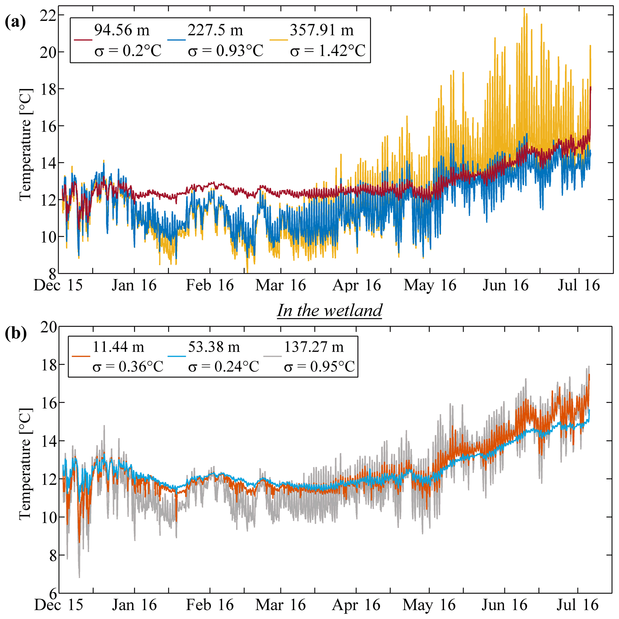
Figure 5Examples of streambed temperature variations measured with the FO-DTS (a) at 94.56, 227.5, and 357.91 m from upstream, with respective SD values equal to 0.2, 0.93, and 1.42 ∘C. (b) In the wetland area at 11.44, 53.38, and 137.27 m from upstream, with respective SD values equal to 0.36, 0.24, and 0.95 ∘C.
Streambed temperature measurements clearly show a general trend, with an increase in the amplitudes of temperature variations measured from upstream (the spring) to downstream, up to around 300 m. In the first 300 m, temperature fluctuations appear attenuated compared to the daily temperature fluctuations and the streambed temperature variations measured more downstream (beyond 300 m). Thus, lower temperature amplitude variations suggest groundwater inflows, especially for the measurement points where the lowest values of SD are recorded (minimal spikes of SD digressing from the general trend, as illustrated by the blue line in Fig. 5b). Indeed, for these hotspots, thermal anomalies are clearly recorded, and the temperature is relatively stable over time, according to the stable groundwater temperature (around 12.5–13 ∘C). The general increase in SD from the spring up to 300 m may be associated to a global decrease in groundwater inflows from upstream to downstream in the first 300 m of the watershed. Higher and very localized inflows would be located in spots where the value of the SD is clearly lower than the general trend. Nevertheless, the gradual increase of the SD could also be alternatively explained by the fact that the stream water temperature, equal to the groundwater temperature at the spring, may progressively equilibrate with the air temperature when travelling along the stream.
To summarize, hotspots associated to minimal spikes of SD are certainly associated to local groundwater discharges, but the general evolution of temperature SD may be due to different factors.
3.1.2 Quantifying groundwater/stream water exchanges
To go further into the interpretation of streambed temperature variations, the FLUX-BOT model was applied for each measurement point. A detailed example of the application of the FLUX-BOT model on a single measurement point (d= 5.08 m), including the quality criteria associated to the fluxes estimates, is presented in Fig. S3. Although the model was applied for each measurement point, simulated temperature variations are consistent only with DTS measurements located in the first 150 m of the temperature profile (SD < 1 ∘C), with NSEs > 0.74, R2 > 0.85 and RMSEs < 0.9 ∘C. Beyond 150 m, the quality of the results decreases considerably, with NSEs < 0.6, R2 < 0.65 and RMSEs > 1.8 ∘C. Thus, the uncertainties on fluxes estimates are too large in this lower part of the watershed (for d > 150 m) to estimate groundwater discharge. Consequently, the model is found not applicable for interpreting temperature measurements, and the results are not provided here.
Figure 6 shows the results of the application of the FLUX-BOT model on passive DTS measurements collected along the cable deployed in streambed sediments in the wetland area, for d < 150 m, where the model is applicable. The model predicts negative values of fluxes all along the interpreted section, indicating upward water flow, which strengthens the assumption of groundwater discharge into the stream. However, as shown in Fig. 6b, groundwater flux estimates are strongly dependent on the value of thermal conductivity of the sediments used in the model. By varying the thermal conductivity from 1 W m−1 K−1 (blue line) to 4 W m−1 K−1 (green line), the estimated discharge is around 4 times higher. For instance, at d= 75 m, the mean flux is estimated m s−1 for λ= 1 W m−1 K−1 against m s−1 for λ= 4 W m−1 K−1. Note, however, that the results are more sensitive to the value of the thermal conductivity when groundwater inflows are higher (see Fig. S3 for more details).
Regardless of the uncertainties, the model also predicts a general decrease in groundwater discharge from upstream to downstream. Higher groundwater inflows are estimated upstream at the head of the catchment and close to the spring (Fig. 6b). The inflows are estimated as twice as high near the spring than downstream. Hence, assuming a thermal conductivity of the sediments λ= 2.5 W m−1 K−1 (orange line in Fig. 6b), the mean flux is estimated m s−1 near the spring (d= 0 m), while it only reaches m s−1 for d= 150 m. The comparison with the SD profile (Fig. 6a) tends to confirm the correlation between the value of the SD of streambed temperature and the importance of groundwater discharge. Results also suggest that local spikes of SD (at 95 or 100 m, for instance) can be associated to preferential pathways, where groundwater discharge is locally estimated four times higher than elsewhere.
Finally, Fig. 6c shows the evolution in time of groundwater discharges estimated for six different measurement points, assuming thermal conductivity λ= 2.5 W m−1 K−1. The variability in fluxes is greater from January to May, with groundwater inflows varying between and m s−1. Lower groundwater inflows are detected during the first month of the experiment ( m s−1) and at the end of the experiment ( m s−1), which seems consistent with stream gauging evolution. The same temporal dynamic is observed for all data collected in the wetland area.
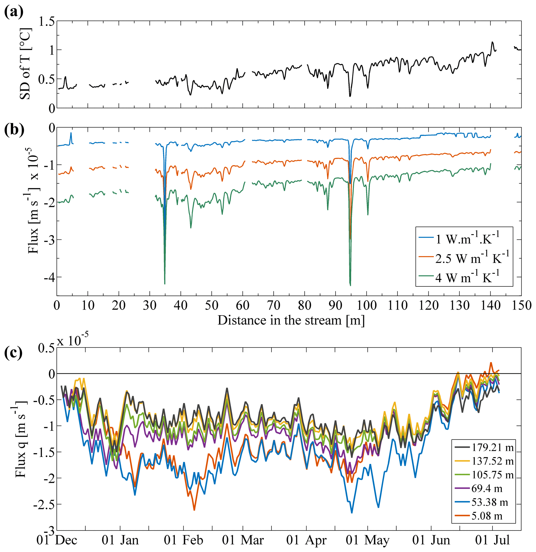
Figure 6(a) Profile of the SD of the streambed temperature calculated over the experiment duration for each measurement point located along the FO cable and deployed in the wetland area. (b) Profiles of mean fluxes estimated over the experiment duration using the FLUX-BOT model from DTS measurements collected in streambed sediments in the wetland area, considering three values of thermal conductivity (negative values indicate an upward water flux). (c) Temporal evolution of the estimated flow considering λ= 2.5 W m−1 K−1.
3.2 Active DTS measurements
3.2.1 Data interpretation
As explained in Sect. 2.3, some measurements points were excluded from the analysis either because the heated FO cable could not have been correctly buried or because temperature measurements were not representative of the effective temperature signal. The data interpretation was thus focused on the selected significant data points as shown in Fig. 7a. This figure presents the increase in temperature ΔT measured 3.45 h after the start of the heat experiment. We recall that the temperature rise ΔT(t) measured during active DTS experiments depends on the thermal conductivity of the sediments which controls the rate of increase through time and on groundwater flow, which limits the temperature rise (Simon et al., 2021a). Despite some areas without data, the values of ΔT measured 3.45 h after the start of the heat experiment are distributed over less than 55 m, offering a large view of the variability in thermal responses. The value of ΔT is particularly variable and ranges between 19.42 ∘C (at 11.2 m) and 36 ∘C (at 132.5 m). However, despite the variability observed, adjacent points present, in general, a similar dynamic with similar values of ΔT, suggesting similar behaviours over a certain range or scale.
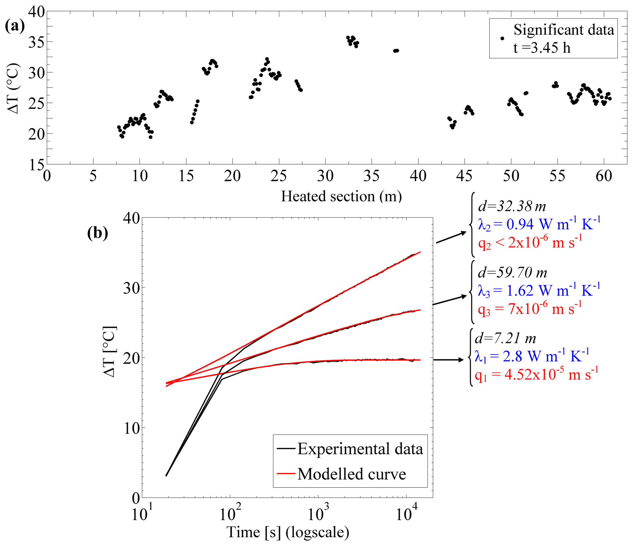
Figure 7(a) Significant ΔT values measured 3.45 h after the start of the heating period measured along the buried FO section. (b) Examples of data interpretation on three thermal response curves observed in the data (black lines). The MILS model was used to reproduce the temperature increase during both the conduction- and advection-dominant periods (red lines).
Each data point was interpreted using the ADTS toolbox to estimate thermal conductivities and fluxes. Figure 7b shows three examples of thermal response curves observed in the data collected along the heated FO section (black lines) and their respective interpretation with the ADTS toolbox (red lines). The data interpretation focuses on the interpretation of the second part of the temperature increase (for t > 90 s) corresponding to the temperature increase controlled by heat conduction and advection in the sediments (Simon et al., 2021a). As illustrated in Fig. 7b, the thermal conductivity highly controls the thermal response and the variability in ΔT. For instance, at d= 32.38 m, the temperature rise reaches 34.7 ∘C after 3.45 h of heating, which is in concordance with the very low thermal conductivity estimated (0.94 W m−1 K−1). On the contrary, at d= 7.21 m, where the temperature rise is much lower and reaches only 19.7 ∘C, λ is estimated at 2.8 W m−1 K−1. The fluxes are then estimated using the temperature at later times, as the intensity of the flux controls temperature stabilization (Simon et al., 2021a). Thus, for instance, the following fluxes values of and m s−1 are estimated at d= 59.70 and d= 7.21 m, respectively. However, for some points, as illustrated by the temperature evolution measured at d= 32.38 m, the temperature does not stabilize for later times and keeps increasing with no inflexion over the whole heating period. This implies either no-flow conditions (q= 0 m s−1) or very low-flow conditions which imply that the heat duration was not long enough to reach temperature stabilization (Simon et al., 2021a). In these cases, only an estimate of qlim can be provided, which corresponds to the highest value of flow that would induce such temperature increase. For instance, at d= 32.38 m, the flux is estimated to be lower than m s−1.
3.2.2 Spatial variability in thermal conductivities and water fluxes estimates
Figure 8 shows the estimation of both the thermal conductivities (Fig. 8a) and the fluxes (Fig. 8b) obtained from active DTS measurements using the ADTS toolbox. It provides an estimate of their respective spatial distribution at a very small scale. As shown in Fig. 8a, the thermal conductivities estimated along the heated section vary between 0.8 and 3.14 W m−1 K−1, with a median value at 1.65 W m−1 K−1. The RMSE calculated between observed data and the best fit model was systematically lower than 0.05 ∘C. Seeing the data noise (< 0.1 ∘C), the maximal uncertainty of these estimates is estimated to be ±0.2 W m−1 K−1.
As shown in Fig. 8b, estimated groundwater fluxes vary between and m s−1, with a mean value at m s−1 and a SD of m s−1. For nine locations (blue points), only the value of qlim was evaluated since the departure of the conduction regime towards temperature stabilization was not reached at the end of the heating period. Note that the data interpretation does not provide the flow direction, as the temperature increase is identical for upward and downward conditions. Although significant measurements are not available all along the sections, results show a decrease in the flux from upstream to downstream, particularly in the first 20 m of the measurements. At greater distances, fluxes are more diffuse in space, except at few locations, for instance at 43, 50, and 52 m from the start of the heated section where higher values are observed. Interestingly, very local and high fluxes values, spreading on less than 2 m, can be observed, as, for instance, at d= 10 m.
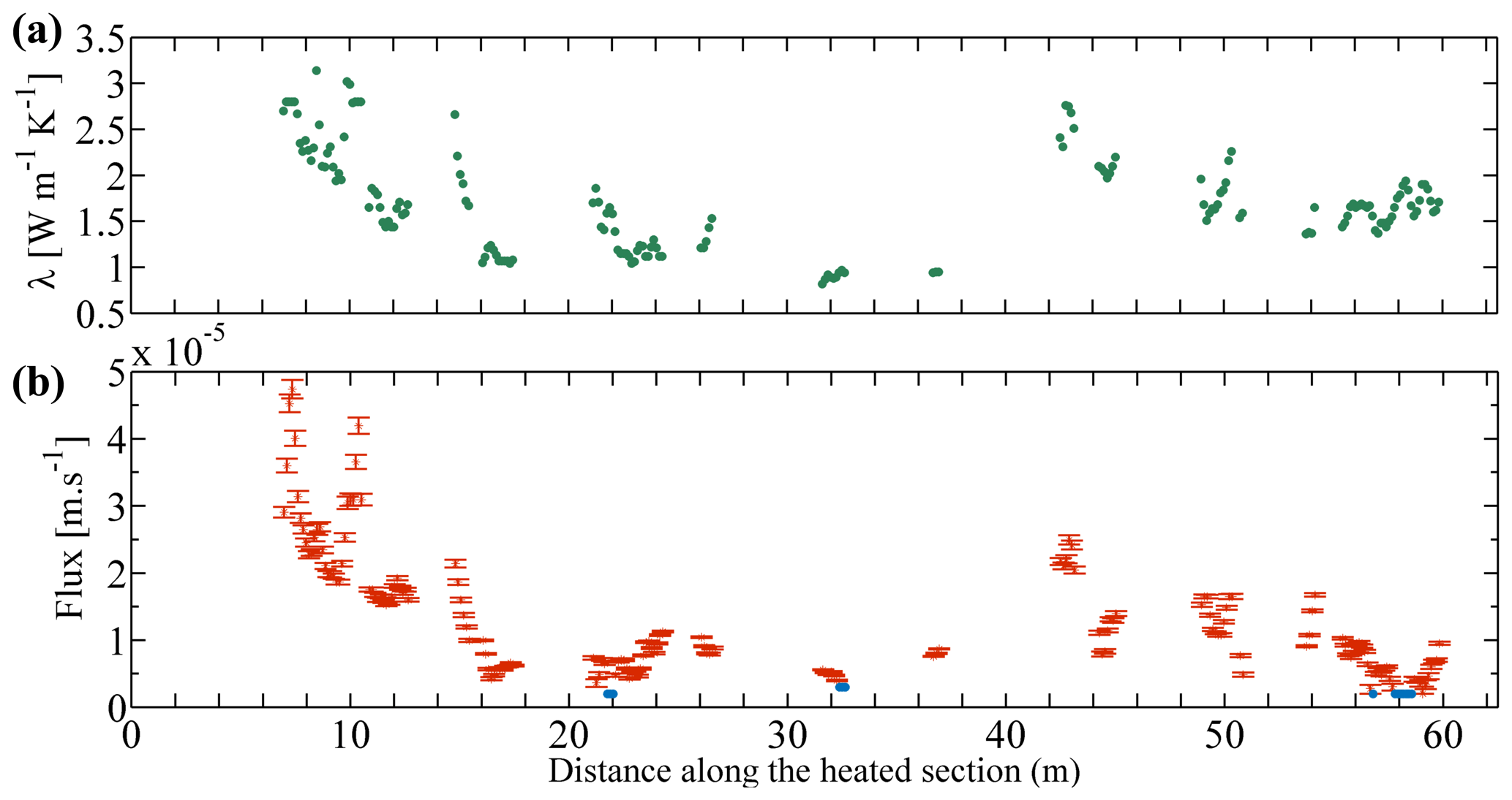
Figure 8The interpretation of active DTS measurements along the heated section of FO cable leads to the estimation of the spatial distribution of both (a) the thermal conductivity (uncertainty = ±0.2 W m−1 K−1) and (b) the water fluxes and their associated errors (error bars). Blue points mark locations where the temperature stabilization is not reached and where an estimate of qlim is provided. Errors bars corresponding to uncertainties on flow estimates calculated with respect to data noise for each measurement points are shown.
3.3 Comparison between passive and active DTS measurements
Figure 9 compares estimated values of groundwater fluxes for 7 April 2016. The flow direction is assumed upward in agreement with passive DTS measurements (Fig. 6b).
For passive DTS measurements, the two light grey curves correspond to flux estimates considering λ= 1 and λ= 4 W m−1 K−1, assuming that the effective values of fluxes should range between these two estimates. The estimation of groundwater discharges clearly remains highly uncertain because of the lack of knowledge about thermal conductivity variations. Results nevertheless show a slight decrease in groundwater discharge from upstream to downstream, but the high uncertainty probably blurs the actual trend.
On the contrary, flux estimates from active DTS measurements (pink points) present a much smaller uncertainty (Fig. 9), confirming the interest of using a heat source to improve fluxes measurements. Flux estimates from both passive and active DTS measurements roughly agree, but active DTS measurements reveal a larger spatial variability regarding groundwater discharge. Interestingly, flux estimates from active DTS measurements can be qualitatively compared with the evolution of the SD of temperature (green line). The lowest SD values are located in the first 55 m of the stream, which is in good agreement with the active DTS measurements that highlighted highest groundwater discharges between 47 and 53 m (between and m s−1). Between approximately 55 and 60 m, the value of the SD increases rapidly (from 1.25 ∘C at 54 m to 2 ∘C at 60 m), while the fluxes estimated from active DTS measurements decrease linearly (from at 56.8 m to m s−1 at 58.5 m). From 60 m, the SD increases and the associated values of fluxes estimated from active DTS are particularly low, varying, for instance, between and m s−1. Interestingly, the locations of the local increases in groundwater discharge detected with the active experiment at 87.5, 95, and 100 m (black arrows) match well with isolated decreases in SD values. Note also that flux estimates from active DTS measurements are in very good agreement with the results of VTPs (blue line). The estimated flux based on passive DTS measurements at 53.4 m is also in good agreement with active DTS results, despite the large uncertainty.

Figure 9Comparison of flow estimated the 7 April 2016 using the vertical temperature profiles (VTPs), the passive DTS measurements, and the active DTS measurements. Results are compared with the evolution of SD of the temperature calculated from passive DTS measurements. The black arrows highlight localized groundwater discharge.
Theoretically, considering the effective value of thermal conductivity in the model, this should highly improve the results obtained from passive DTS measurements. Thus, the thermal conductivity estimates provided from active DTS measurements were used to fully re-interpret the passive DTS measurements using the FLUX-BOT model. As a result, the estimated range of fluxes was highly reduced and was found to be in much better agreement with other estimates, as shown by dark grey lines in Fig. 9. For instance, between 63 and 72 m, the thermal conductivity was evaluated from active DTS measurements between 1 and 1.9 W m−1 K−1, depending on measurement points (Fig. 8a). Using such values, the fluxes estimated from passive DTS measurements in this area vary between and m s−1 (dark grey lines), whereas they were initially estimated between and m s−1, considering λ between 1 and 4 W m−1 K−1 (light grey lines). As shown in Fig. 9, except between 48 and 52 m where small discrepancies remain, this approach significantly reduces the range of fluxes estimated and shows that passive DTS results are in good agreement with active DTS results when an independent and more precise estimate of the thermal conductivity is considered.
In the following, we discuss the advantages and limitations of applying either passive or active DTS experiments, depending on the objectives of the study and on technical limitations. Thus, we first focus on the possibilities of detecting and localizing groundwater inflows and their spatial and temporal dynamics before discussing the ability of quantify groundwater discharges. Besides comparing both approaches, we show the interest of combining both methods to infer the spatial and temporal variability in groundwater discharge at the catchment scale.
4.1 Detecting, localizing, and monitoring groundwater discharge
Results show that long-term passive DTS measurements turn out to be an efficient method to detect, locate, and monitor thermal anomalies that can be further interpreted as marker of groundwater discharge. The approaches consisted of burying a FO cable in the streambed along several hundreds of metres in order to record streambed temperature variations at high resolution during several months. The high spatial and temporal resolution of measurements is clearly the main advantage of the passive DTS experiment, since such an achievement would not have been possible with individual temperature probes. Moreover, although the FO installation in the streambed can be difficult, depending on the streambed nature, the long-term recording of temperature is relatively easy and autonomous.
Streambed temperature measurements recorded with the FO cable allow the first assumptions about the spatial and temporal dynamics occurring in the watershed, if used over a several-months-long monitoring period, to be made. To do so, the calculation of the standard deviation (SD) of streambed temperature over time appears to be a reliable proxy for locating inflows (Figs. 4 and 5), since lower SD values reflect a larger attenuation of daily temperature amplitudes. Here, the SD of temperature increases progressively from upstream to downstream, until reaching the SD of stream temperature at around d= 300 m (Fig. 4b). Very localized and low values of SD, described previously as minimal spikes of SD digressing from the general trend, also appear along the profile. Theoretically, temperature variations recorded in the streambed depend on the stream temperature variations and on the intensity of stream water/groundwater exchanges (Constantz, 2008). Interpreting the data without measuring stream temperature variations along the stream requires the assumption that the stream temperature is uniform along the investigated section. In this case, the value of SD of the stream temperature can be assumed to be uniform as well along the investigated section, and any value of SD measured in the streambed lower than the SD of the stream temperature could actually be interpreted as the result of groundwater inflows. Here, this assumption seems reasonable, since shade and lighting conditions, as well as water depths, are very similar along the investigated section. Moreover, the transit time from the spring to the gauging station is relatively rapid due to the short distances. The river slopes and the low water depths imply a fast balance between the air temperature and the stream temperature. This assumption is partly confirmed with the stream temperature recorded near the spring with the DTS in an area where the FO cable is not buried but lies at the bottom of the stream. At this location, the SD of the temperature equals 1.03 ∘C, which is a little less than 1.375 ∘C, which is the value recorded in the stream at the gauging station E30, located at around 490 m in the spring. However, this suggests that the SD of the stream temperature signal should be relatively high, greater than 1 ∘C all along the stream and, consequently, much larger than the SD recorded within the streambed, especially in the upstream section of the stream (first 300 m).
Consequently, results suggest a decrease in groundwater inflows from upstream to downstream in the first 300 m of the watershed, with higher and localized inflows in spots characterized by SD values clearly lower than the general trend. This is strengthened by the fact that the lowest values of SD (minimal spikes of SD illustrated by the blue line in Fig. 5b) correspond to clear thermal anomalies for which the temperature appears relatively stable over time. Beyond 300 m, the values of the SD are almost equal to the SD of the stream temperature, and the recorded temperature variations are approximately similar to the stream temperature variations. Concerning the second part of the golf course area (from 300 to around 470 m), the data interpretation remains difficult because of the hard substrate that limited the burying of the FO cable. However, in the last 70 m of the FO cable (wood plain), the cable was easily buried in a thick, sandy riverbed. Thus, values of SDs in this area are equal to the one recorded in the stream and would suggest the absence of groundwater inflows, which would remain limited to the wetland and, therefore, to the upper part of the watershed with highest topographic changes, as we shall discuss below.
Active DTS measurements could also be used for localizing inflows, since the approach allows for the accurate quantification of groundwater fluxes. However, contrary to passive DTS measurements that can be easily used to provide groundwater discharge areas, their identification from active DTS measurements requires going through flux quantification, which can be more constraining. Moreover, this method requires more instrumentation, and the length of the heated section is limited depending on the power supply available (Simon et al., 2021a). Thus, flow investigation at the watershed scale is way more difficult to achieve unless multiplying the installation of heated sections in the streambed. Furthermore, active DTS measurements provide a punctual estimate of fluxes. To characterize the temporal dynamics of flow, these experiments must be repeated often, which is clearly more constraining than conducting long-term passive DTS measurements because active DTS experiments require more instrumentation (heat pulse system, electrical cables, etc.). However, the repetition of active DTS measurements offers very promising perspectives for environmental monitoring, as recently shown by Abesser et al. (2020), who repeated surveys under different meteorological or hydrological conditions in order to monitor the evolution of thermal and hydraulic properties of the soil subsurface.
4.2 Quantification of groundwater discharge
4.2.1 About the large uncertainties associated to the interpretation of passive DTS measurements
The inverse numerical FLUX-BOT model was used to quantify the vertical fluxes from passive DTS measurements in the first 150 m of the temperature profile, which represents 545 measurements points. Although this approach provided fluxes estimates, their relevance can clearly be discussed. Indeed, the estimates are highly uncertain, which demonstrates the difficulty of quantifying groundwater fluxes using passive DTS measurements recorded along a single FO cable. The large uncertainties on estimates are due to several sources of uncertainties. First, the model relies on the comparison of temperature variations recorded at three different depths. Ideally, the approach would require deploying at least three FO cables in the field (Mamer and Lowry, 2013) in order to continuously measure temperature conditions at high resolution at upper and lower boundaries, which was technically impossible in the field. Thus, as discussed above, the stream temperature variations were assumed to be uniform along the studied section, which seems consistent here. Moreover, the temperature signal recorded in the piezometer F4 was used to set the lower boundary condition of the model. This piezometer seems to be a good proxy for groundwater temperature, since the temperature signal measured at 20 m depth in the piezometer F5b is similar to the one measured at 15 m depth in the piezometer F4. This also suggests that the temperature of groundwater discharging into the stream is uniform along the investigated portion of the catchment. However, although the assumptions about stream and groundwater temperatures seem reasonable, it considerably increases the uncertainties on fluxes estimates. Second, the model requires defining the burial depth of the cable to calculate vertical fluxes while results are very sensitive to this parameter. Complementary tests (not shown here), conducted by varying the depth of the FO cable in the model, suggest that varying the burial depth by ±2 cm induces, on average, a difference of ±50 % on fluxes estimates, showing the high uncertainty associated to the uncertainty on burial depth. Last but not least, results showed that thermal conductivity values have a very strong impact on fluxes estimates, which is consistent with the results of Briggs et al. (2014), Duque et al. (2016), Lapham (1989), and Sebok and Müller (2019). The lack of knowledge and assumptions on thermal conductivities values lead to high uncertainties on fluxes estimates using both VTP and passive DTS measurements (Fig. 6b). In situ estimates of thermal conductivities using thermal conductivity probes could considerably improve the fluxes estimates, as demonstrated by Duque et al. (2016), who reported an up to 89 % increase in flux estimates when using in situ measured sediment thermal conductivities. However, on seeing the high spatial variability in the thermal conductivity highlighted through the active DTS experiment, it would certainly require a tremendous effort in the field to characterize such a variability with single probes. Moreover, it will not remove others sources of uncertainties associated to the burial depth of the FO cable or the lack of temperature measurements at different depths all along the section.
Consequently, uncertainties on fluxes estimates are so large that a passive DTS experiment does not appear to be a reliable and accurate method for estimating seepage rates. However, in the first 150 m, the model allows the determination of the flow direction (upwelling fluxes), demonstrating that thermal anomalies can definitely be associated to groundwater inflows confirming the spatial and temporal dynamics of exchanges occurring in the wetland. Note that the model was not even applicable in the lower part of the watershed (for d > 150 m) to estimate flow direction. Thus, despite the values of the SD recorded between d= 150 and d=300 m, suggesting potential groundwater inflows, groundwater inflows are probably too low or diffuse in this part of the watershed to apply the model and validate even the flow direction.
To summarize, fluxes quantification from passive DTS measurements depends on several assumptions about thermal properties and boundary conditions, which induces high uncertainties on fluxes estimates. Burying a single FO cable in the streambed, although very promising and interesting, is limited to fully characterizing and quantifying groundwater/surface water interactions, even in a headwater watershed. For further applications, results suggest the necessity for deploying an additional FO cable at the bottom of the stream in order to also measure stream temperature variations at high resolution all along the studied section. This seems to be the only way to fully and efficiently extend the thermal-based classical methods (Constantz, 2008; Hatch et al., 2006) at a high spatial resolution. A third buried FO cable would be the optimal configuration to estimate distributed vertical fluxes (Mamer and Lowry, 2013) and reduce the uncertainties on fluxes estimations based on passive DTS measurements.
4.2.2 Accuracy of fluxes estimated with active DTS measurements
Contrary to passive DTS measurements, the active DTS measurements turn out to be an efficient method to estimate fluxes. From only 4 h of measurements, the approach provides an estimate of both the thermal conductivities and the fluxes along the heated cable, confirming the high variability in these two parameters in space (Fig. 8). Despite some difficulties with installing the heated FO cable, fluxes were nevertheless estimated for 172 measurements points along a 60 m section of cable, which is an excellent performance. This high resolution is particularly interesting for the characterization of spatial variabilities at a small scale. Such results cannot be achieved with any other methods commonly used in this context. Note that the installation of the heated FO cable was entirely manual and rapid, which probably partly explains the relatively large number of measurement points removed from data processing. Nevertheless, the use of tools like ploughs should improve the burying of the cable, limit the alteration of the riverbed, and allow for a much better control of the burial depth.
Results show that streambed thermal conductivities are relatively variable in space, typically between 0.9 and 3.1 W m−1 K−1 (Fig. 8a), which is consistent with streambed sediments composed of saturated clay and silt and saturated sand and gravel, whose thermal conductivity values commonly range respectively between 0.9 and 4 W m−1 K−1 (Stauffer et al., 2013). The large range of thermal conductivities observed in this relatively small section of streambed (less than 60 m) demonstrates the interest in distributed measurements for characterizing streambed heterogeneity. No other method could provide an estimate of the thermal properties at this spatial resolution.
Groundwater fluxes were estimated between and m s−1, which is in very good agreement with the results of the VTPs (Fig. 9). The results suggest a decrease in the groundwater discharge from upstream to downstream, with the most significant inflows located in the first 20 m of the heated section. Elsewhere, groundwater discharge is more diffuse in space, although significant groundwater discharge areas can be locally observed. These local increases in groundwater discharge match with isolated decreases in streambed temperature SD values, calculated from passive DTS measurements (Fig. 9). This confirms the possibility of investigating very local groundwater inflows and the capability of investigating the spatial evolution of fluxes at a very small scale.
The magnitude of groundwater flux is also in good agreement with the measured stream flow. Considering the width and the length of the investigated stream where groundwater inflows have been estimated, the contribution to the stream can be roughly evaluated at around 4 L s−1. This means that 57 % of the stream flow at the time of the experiment was contributed by groundwater, knowing that the average flow measured at the downstream gauging station was 7 L s−1 for this period.
It clearly appears that the main advantages of the approach are (i) the low uncertainty on fluxes estimates and (ii) the associated estimates of thermal conductivities. The use of the ADTS toolbox that automatically interprets active DTS measurements (Simon and Bour, 2022) highly facilitates the data interpretation, which is finally much easier than the interpretation of passive DTS measurements. Contrary to passive DTS measurements, the interpretation of active DTS measurements provides estimates of thermal conductivities with a very good accuracy. Thus, the approach does not require the assumption of thermal conductivity values, which considerably reduce the uncertainties in the fluxes estimates. However, the burial depth of the heated cable might potentially affect the thermal response if the cable is too close to the stream. In this case, the stream temperature could limit the temperature elevation by dissipating the heat produced, and further investigations should be done to quantify the effect of the nearby stream on estimates. However, here, the active DTS experiment was conducted straight after the installation of the cable, ensuring that the burial depth was sufficient to limit the effect of the nearby stream (results from modelling showed that the heating is particularly localized around the heated cable). Finally, in gaining streams, active DTS measurements are independent of temperature boundary conditions, as long as the groundwater temperature is constant over time. Indeed, in gaining conditions, with no groundwater temperature variations, the temperature evolution measured along the FO cable is exclusively due to heat injection, streambed sediment properties, and groundwater flow intensity. Here, over the heating experiment, an average temperature of 12.1 ∘C, with a standard deviation of 0.12 ∘C, has been recorded in sediments along the non-heated buried sections of the cable, demonstrating that the streambed temperature was not affected by potential air/stream variations and that the temperature variations recorded along the heated section are exclusively due to the heat experiment. In losing conditions, since diurnal water temperature variations propagate deeper, it could be necessary to separate the temperature evolution induced by the heat injection from the one depending on stream temperature variations.
4.2.3 About the complementary use of both approaches
Finally, the complementary use of both approaches should be noted. First, the data interpretation of active DTS measurements does not provide the flow direction, contrary to the interpretation of passive DTS measurements. Note that the temperature variations recorded before the heating period and after the end of the recovery can be used to determine the flow direction as soon as the stream temperature variations are assumed to be uniform along the heated section. Of course, results of active DTS measurements are useful for validating the general behaviour/trend highlighted through passive DTS measurements, which is a baseline of groundwater discharge associated to local and important spikes of discharge. They do not fully allow the validation of the different hypothesis made to interpret passive DTS measurements, but they permit checking the consistency of the results obtained. Results also show (Fig. 9) that the interpretation of active DTS measurements can be directly used to improve the interpretation of passive DTS measurements. Indeed, the values of thermal conductivities, estimated from active DTS measurements, can be used to calibrate the inverse model and, therefore, to reduce the uncertainties on fluxes estimates from passive DTS measurements. This is a very promising result, since it highly facilitates the interpretation of passive DTS measurements. Once thermal conductivity distribution is known along the section, passive DTS experiments could, therefore, be considered as an independent and full tool to quantify GW discharge at high resolution through long-term monitoring (although the assumption on the stream temperature remains an issue).
Moreover, note also that, for the interpretation of both passive and active DTS measurements, the flow is assumed to be vertical and perpendicular to the FO cable. Although flow is generally assumed to be vertical when using heat as a tracer for studying groundwater/stream interactions (Constantz, 2008; Hatch et al., 2006; Lapham, 1989), nonvertical fluxes can affect natural temperature profiles and associated fluxes estimates (Bartolino and Niswonger, 1999; Cranswick et al., 2014; Cuthbert and Mackay, 2013; Lautz, 2010; Reeves and Hatch, 2016). Obviously, like for most thermal-based methods, this is a main limitation when using passive DTS measurements to detect and quantify groundwater discharge. Likewise, nonvertical fluxes could also affect the interpretation of active DTS measurements. Thus, some studies suggest that the impact of the angle of the flow against the cable is significant as soon as it differs by more than ± 30∘ from being perpendicular (Aufleger et al., 2007; Chen et al., 2019; Perzlmaier et al., 2004).
4.3 Characterizing groundwater discharge dynamics
The complementary use of these two DTS approaches allows the characterization of spatial and temporal patterns of groundwater discharge in this headwater catchment. Results and associated flux estimates are consistent with previous studies that predicted that 80 %–90 % of the stream flow was induced by groundwater discharge (Fovet et al., 2015b; Martin, 2003). Interestingly, the two approaches allow the characterization of the groundwater discharge dynamic at two different scales. This is a particularly promising and exciting achievement, since groundwater/surface water interactions are generally controlled by multi-scale processes, making their characterization particularly challenging in the field (Brunke and Gonser, 1997; Fleckenstein et al., 2006; Flipo et al., 2014; Harvey and Bencala, 1993; Kalbus et al., 2009).
First, conducting measurements over more than 530 m allow for the description of the groundwater discharge dynamic at the catchment scale. Thus, results suggest that the groundwater contribution is localized at the very head of the catchment, which is in the upstream near the spring where the steepest slopes can be observed. Further downstream, beyond 60 m from the spring, the groundwater discharge decreases progressively and rapidly. This confirms the importance of the topography in the stream generation in headwater area (Harvey and Bencala, 1993; Sophocleous, 2002; Tóth, 1963; Winter, 2007) and the role of local topography variations in groundwater discharge (Baxter and Hauer, 2000; Flipo et al., 2014; Frei et al., 2010; Jencso et al., 2009; Stonedahl et al., 2010; Tonina and Buffington, 2011; Unland et al., 2013).
Second, the high resolution of DTS measurements allows us to study the groundwater discharge dynamic at a very small scale, and thus highlight local heterogeneities, which would not have been possible with more integrative methods. Therefore, beyond the role of topography, which acts as the main driver of groundwater inflows, variations in hydraulic conductivity could also explain the presence of local hotspots with high groundwater inflows, as highlighted by both methods in the wetland area, which is upstream near the spring. Indeed, these hotspots or spikes that would highly contribute to the stream flow may be driven by local changes in the hydraulic gradient, induced by the successive streambed topography changes but are more likely due to hydraulic properties changes, given the amplitude and scale of the variations. Such hydraulic conductivity variations could come from uneven bedrock weathering or the presence of fractures, which is very common in such bedrock geology (Buss et al., 2008; Guihéneuf et al., 2014). Such heterogeneities may control flow in the subsurface but can also influence the nature of the streambed. This would also explain why the values of the fluxes seem correlated, at least at some places, with the values of thermal conductivities (Fig. 8). Indeed, our results suggest that local hotspots with high groundwater inflows are also associated to higher values of thermal conductivities. This is consistent with a change in streambed properties. Indeed, clay and silt have much lower hydraulic conductivities than sand but also lower thermal conductivities (Stauffer et al., 2013). Although cross-correlation analysis would be useful to take the interpretation further, such correlation would not be surprising, since the nature of the streambed affects both its hydraulic conductivity and its thermal properties.
Concerning temporal variations, three different time periods were clearly identified from the passive DTS measurements according to the behaviour of the streambed temperature evolution over time (Figs. 4 and 5). The increase in precipitations in winter certainly leads to a gradual increase in the hydraulic gradient, which induces groundwater exfiltration into the stream once the elevation of the groundwater table becomes higher than the elevation of the stream stage. In spring, the groundwater table decreases progressively, and so does the groundwater contribution to stream flow. Since changes in the piezometric levels are periodic, with alternating periods of high and low water table levels, we can assume that exchanges have a similar temporal dynamic from year to year, which can help in managing the water resources. These results are consistent with the temporal dynamic of exchanges observed under a temperate climate, where the intensity of groundwater/surface water exchanges fluctuates according to seasonal patterns (Brunke and Gonser, 1997; Sophocleous, 2002). More importantly, these results highlight the interest of the long-term monitoring of streambed temperature with DTS. Here, with only 8 months of measurements, the experiment allowed us to continuously monitoring hydrological conditions changes and clearly identify hotspots corresponding to groundwater discharge periods. In headwater catchments, these tools should allow, in the near future, for the investigation of the distribution of response times of groundwater discharges to some specific events, which is very promising.
Passive and active DTS measurements were conducted concurrently at the same experimental site in order to characterize the spatial and temporal patterns of groundwater discharge into a first- and second-order stream. Long-term passive DTS monitoring can easily be used to assess the spatial and the temporal dynamics of groundwater discharge. The analysis of the streambed temperature recordings allows us to identify the thermal anomalies that can be interpreted as markers of groundwater inflows into the stream. Here, results suggest that groundwater discharge is localized in the upper part of the watershed where topographic gradients are the highest.
However, this study also demonstrates the limitations of passive DTS measurements for quantifying groundwater discharges. When a single FO cable is buried in the streambed, the data interpretation requires making strong assumptions about the thermal conductivity of sediments and about the stream temperature. Uncertainties may be reduced if previous and independent measurements of the variability in streambed thermal conductivities are conducted through active DTS measurements. Nevertheless, the interpretation of passive DTS measurements would still rely on the assumption that the stream temperature is uniform along the studied section. In practice, the proper estimation of passive DTS measurements conducted in streambeds would require measuring the stream temperature with the same spatial resolution and, thus, deploying a second FO cable at the bottom of the stream.
Active DTS measurements allowed further characterization of the groundwater inflows through estimating the fluxes and their spatial distribution with a very low uncertainty in comparison with passive DTS measurements and in situ thermal methods. The quantification of groundwater fluxes through the active DTS measurements clearly shows the co-existence of both local hotspots, characterized by very localized and high groundwater inflows, and more diffuse groundwater inflows elsewhere along the heated section. This allowed us to confirm the role of topography on the large-scale variations in groundwater discharge but also the role of heterogeneities at small scales. Such small-scale variability in groundwater discharge is certainly associated to hydraulic conductivity variations. Moreover, the active DTS experiment allowed us to describe the high variability in thermal conductivity in space
Finally, it should be noted that passive DTS measurements permitted us to locate the spatial and temporal patterns of groundwater inflows on relatively large distances, while active DTS measurements allowed a much more precise and robust estimate of both thermal conductivities and fluxes which can highly contribute to improve passive DTS methods interpretation. Hence, the combination of active and passive DTS methods provided an imaging of the spatial variability in groundwater inflows. It allowed us to better infer the role of topography, which acts as the main driver of groundwater inflows in the upper part of the watershed, and also the impact of hydraulic conductivity variations, which may explain the presence of very localized and high groundwater inflows.
Thus, these methods, and especially active DTS measurements, conducted in the streambed open very promising perspectives for a novel characterization of the groundwater/stream interfaces, especially if surveys are repeated under different meteorological or hydrological conditions. Being able to continuously monitor the temporal dynamic of exchanges is a very promising achievement that could be useful for understanding the hydrological behaviour in the watershed but also for characterizing the distribution of response times of groundwater discharge. This can be particularly useful for studying biogeochemical hotspots and hot moments (Krause et al., 2017; Singh et al., 2019; Trauth and Fleckenstein, 2017) or to couple this approach with natural tracers to assess the residence times in the hyporheic zone (Biehler et al., 2020; Liao et al., 2021).
The data presented in this study are available online. The data related to the active DTS experiment are available at http://geowww.agrocampus-ouest.fr/geonetwork/apps/georchestra/?uuid=535a3738-0ed7-4376-99f1-9a7a652b893d (Simon et al., 2021b). The data related to the passive DTS experiment are available at http://geowww.agrocampus-ouest.fr/geonetwork/apps/georchestra/?uuid=a5f2a68f-bf63-469c-839b-1e1edf1f8624 (Simon et al., 2021c).
The supplement related to this article is available online at: https://doi.org/10.5194/hess-26-1459-2022-supplement.
NS, OB, LL, OF, and ZT conceptualized the paper. NS curated the data, conducted the formal analysis, developed the methodology and software, visualized the paper, and wrote and prepared the original draft. OB acquired the funding and supervised the project. The investigation was led by NS, OB, NL, MF, OF, HLL, and ZT, while OB, OF, and ZT administered the project. The resources were collected by NL and MF. NS and OB validated the work. NS, OB, OF, ZT, and LL reviewed and edited the paper.
The contact author has declared that neither they nor their co-authors have any competing interests.
Publisher's note: Copernicus Publications remains neutral with regard to jurisdictional claims in published maps and institutional affiliations.
This research has been funded by the Agence de l'Eau Loire Bretagne and by the ANR project EQUIPEX CRITEX (grant no. ANR-11-EQPX-0011).
This research has been supported by the Agence Nationale de la Recherche (grant no. ANR-11-EQPX-0011) and the Agence de l'eau Loire-Bretagne.
This paper was edited by Miriam Coenders-Gerrits and reviewed by Bas F. des Tombe and Stefan Ploum.
Abesser, C., Ciocca, F., Findlay, J., Hannah, D., Blaen, P., Chalari, A., Mondanos, M., and Krause, S.: A distributed heat pulse sensor network for thermo-hydraulic monitoring of the soil subsurface, Q. J. Eng. Geol. Hydroge., 53, 352–365, https://doi.org/10.1144/qjegh2018-147, 2020.
Anderson, M. P.: Heat as a ground water tracer, Ground Water, 43, 951–968, https://doi.org/10.1111/j.1745-6584.2005.00052.x, 2005.
Aufleger, M., Conrad, M., Goltz, M., Perzlmaier, S., and Porras, P.: Innovative dam monitoring tools based on distributed temperature measurement, Jordan Journal of Civil Engineering, 1, 29–37, 2007.
Banks, E., Shanafield, M., and Cook, P.: Induced Temperature Gradients to Examine Groundwater Flowpaths in Open Boreholes, Ground Water, 52, 943–951, https://doi.org/10.1111/gwat.12157, 2014.
Bartolino, J. R. and Niswonger, R. G.: Numerical simulation of vertical ground-water flux of the Rio Grande from ground-water temperature profiles, central New Mexico, U.S. Geological Survey Water-Resources, Investigations Report 99–4212, 39 pp., https://doi.org/10.3133/wri994212, 1999.
Baxter, C. and Hauer, F.: Geomorphology, Hyporheic Exchange, and Selection of Spawning Habitat by Bull Trout (Salvelinus Confluentus), Canadian Journal of Fisheries and Aquatic Sciences, Can. J. Fish. Aquat. Sci., 57, 1470–1481, https://doi.org/10.1139/cjfas-57-7-1470, 2000.
Bencala, K.: A Perspective on Stream-Catchment Connections, J. N. Am. Benthol. Soc., 12, 44–47, https://doi.org/10.2307/1467684, 1993.
Bense, V. F., Read, T., Bour, O., Le Borgne, T., Coleman, T., Krause, S., Chalari, A., Mondanos, M., Ciocca, F., and Selker, J. S.: Distributed Temperature Sensing as a downhole tool in hydrogeology, Water Resour. Res., 52, 9259–9273, https://doi.org/10.1002/2016WR018869, 2016.
Biehler, A., Chaillou, G., Buffin-Bélanger, T., and Baudron, P.: Hydrological connectivity in the aquifer–river continuum: Impact of river stages on the geochemistry of groundwater floodplains, J. Hydrol., 590, 125379, https://doi.org/10.1016/j.jhydrol.2020.125379, 2020.
Brandt, T., Vieweg, M., Laube, G., Schima, R., Goblirsch, T., Fleckenstein, J. H., and Schmidt, C.: Automated in Situ Oxygen Profiling at Aquatic–Terrestrial Interfaces, Environ. Sci. Technol., 51, 9970–9978, https://doi.org/10.1021/acs.est.7b01482, 2017.
Briggs, M. A., Lautz, L. K., and McKenzie, J. M.: A comparison of fibre-optic distributed temperature sensing to traditional methods of evaluating groundwater inflow to streams, Hydrol. Process., 26, 1277–1290, https://doi.org/10.1002/hyp.8200, 2012.
Briggs, M. A., Lautz, L. K., Buckley, S. F., and Lane, J. W.: Practical limitations on the use of diurnal temperature signals to quantify groundwater upwelling, J. Hydrol., 519, 1739–1751, https://doi.org/10.1016/j.jhydrol.2014.09.030, 2014.
Briggs, M. A., Buckley, S. F., Bagtzoglou, A. C., Werkema, D. D., and Lane, J. W.: Actively heated high-resolution fiber-optic-distributed temperature sensing to quantify streambed flow dynamics in zones of strong groundwater upwelling, Water Resour. Res., 52, 5179–5194, https://doi.org/10.1002/2015WR018219, 2016.
Brunke, M. and Gonser, T.: The ecological significance of exchange processes between rivers and groundwater, Freshwater Biol., 37, 1–33, https://doi.org/10.1046/j.1365-2427.1997.00143.x, 1997.
Buss, H. L., Sak, P. B., Webb, S. M., and Brantley, S. L.: Weathering of the Rio Blanco quartz diorite, Luquillo Mountains, Puerto Rico: Coupling oxidation, dissolution, and fracturing, Geochim. Cosmochim. Ac., 72, 4488–4507, https://doi.org/10.1016/j.gca.2008.06.020, 2008.
Carslaw, H. S. and Jaeger, J. C.: Conduction of heat in solids, Second Edition, Oxford University Press, Oxford Science Publication, ISBN 9780198533689, 1959.
Chen, J., Xiong, F., Zheng, J., Ge, Q., and Cheng, F.: The influence of infiltration angle on the identification effect of seepage with linear heat source method, Measurement, 148, 106974, https://doi.org/10.1016/j.measurement.2019.106974, 2019.
Constantz, J.: Heat as a tracer to determine streambed water exchanges, Water Resour. Res., 44, W00D10, https://doi.org/10.1029/2008WR006996, 2008.
Constantz, J. and Thomas, C. L.: The use of streambed temperature profiles to estimate the depth, duration, and rate of percolation beneath arroyos, Water Resour. Res., 32, 3597–3602, https://doi.org/10.1029/96WR03014, 1996.
Cranswick, R. H., Cook, P. G., Shanafield, M., and Lamontagne, S.: The vertical variability of hyporheic fluxes inferred from riverbed temperature data, Water Resour. Res., 50, 3994–4010, https://doi.org/10.1002/2013WR014410, 2014.
Cuthbert, M. O. and Mackay, R.: Impacts of nonuniform flow on estimates of vertical streambed flux, Water Resour. Res., 49, 19–28, https://doi.org/10.1029/2011WR011587, 2013.
del Val, L., Carrera, J., Pool, M., Martínez, L., Casanovas, C., Bour, O., and Folch, A.: Heat Dissipation Test With Fiber-Optic Distributed Temperature Sensing to Estimate Groundwater Flux, Water Resour. Res., 57, e2020WR027228, https://doi.org/10.1029/2020WR027228, 2021.
des Tombe, B. F., Bakker, M., Smits, F., Schaars, F., and van der Made, K.-J.: Estimation of the Variation in Specific Discharge Over Large Depth Using Distributed Temperature Sensing (DTS) Measurements of the Heat Pulse Response, Water Resour. Res., 55, 811–826, https://doi.org/10.1029/2018WR024171, 2019.
Domenico, P. A. and Schwartz, F. W.: Physical and chemical hydrogeology, Second edition, John Wiley & Sons Inc., New York, ISBN 978-0-471-59762-9, 1998
DTS and Accessory Systems: DTS and Accessory Systems, https://ctemps.org/instruments, last access: 31 May 2021.
Duque, C., Müller, S., Sebok, E., Haider, K., and Engesgaard, P.: Estimating groundwater discharge to surface waters using heat as a tracer in low flux environments: the role of thermal conductivity, Hydrol. Process., 30, 383–395, https://doi.org/10.1002/hyp.10568, 2016.
Fleckenstein, J. H., Niswonger, R. G., and Fogg, G. E.: River-aquifer interactions, geologic heterogeneity, and low-flow management, Ground Water, 44, 837–852, https://doi.org/10.1111/j.1745-6584.2006.00190.x, 2006.
Flipo, N., Mouhri, A., Labarthe, B., Biancamaria, S., Rivière, A., and Weill, P.: Continental hydrosystem modelling: the concept of nested stream–aquifer interfaces, Hydrol. Earth Syst. Sci., 18, 3121–3149, https://doi.org/10.5194/hess-18-3121-2014, 2014.
Fovet, O., Ruiz, L., Hrachowitz, M., Faucheux, M., and Gascuel-Odoux, C.: Hydrological hysteresis and its value for assessing process consistency in catchment conceptual models, Hydrol. Earth Syst. Sci., 19, 105–123, https://doi.org/10.5194/hess-19-105-2015, 2015a.
Fovet, O., Ruiz, L., Faucheux, M., Molénat, J., Sekhar, M., Vertès, F., Aquilina, L., Gascuel-Odoux, C., and Durand, P.: Using long time series of agricultural-derived nitrates for estimating catchment transit times, J. Hydrol., 522, 603–617, https://doi.org/10.1016/j.jhydrol.2015.01.030, 2015b.
Fovet, O., Ruiz, L., Gruau, G., Akkal, N., Aquilina, L., Busnot, S., Dupas, R., Durand, P., Faucheux, M., Fauvel, Y., Flechard, C., Gilliet, N., Grimaldi, C., Hamon, Y., Jaffrezic, A., Jeanneau, L., Labasque, T., Henaff, G., Mérot, P., and Gascuel-Odoux, C.: AgrHyS: An Observatory of Response Times in Agro-Hydro Systems, Vadose Zone J., 17, 180066, https://doi.org/10.2136/vzj2018.04.0066, 2018.
Frei, S., Lischeid, G., and Fleckenstein, J. H.: Effects of micro-topography on surface–subsurface exchange and runoff generation in a virtual riparian wetland – A modeling study, Adv. Water Resour., 33, 1388–1401, https://doi.org/10.1016/j.advwatres.2010.07.006, 2010.
Frei, S., Durejka, S., Le Lay, H., Thomas, Z., and Gilfedder, B. S.: Quantification of Hyporheic Nitrate Removal at the Reach Scale: Exposure Times Versus Residence Times, Water Resour. Res., 55, 9808–9825, https://doi.org/10.1029/2019WR025540, 2019.
Gaillardet, J., Braud, I., Hankard, F., Anquetin, S., Bour, O., Dörfliger, N., de Dreuzy, J.-R., Galle, S., Galy, C., Gogo, S., Gourcy, L., Habets, F., Laggoun, F., Longuevergne, L., Borgne, T., Naaim-Bouvet, F., Nord, G., Simonneaux, V., Six, D., and Zitouna, R.: OZCAR: The French network of critical zone observatories, Vadose Zone J., 17, 1–24, https://doi.org/10.2136/vzj2018.04.0067, 2018.
Ghafoori, Y., Vidmar, A., Říha, J., and Kryžanowski, A.: A Review of Measurement Calibration and Interpretation for Seepage Monitoring by Optical Fiber Distributed Temperature Sensors, 20, 5696, https://doi.org/10.3390/s20195696, 2020.
Gilmore, T., Johnson, M., Korus, J., Mittelstet, A., Briggs, M., Zlotnik, V., and Corcoran, S.: Streambed Flux Measurement Informed by Distributed Temperature Sensing Leads to a Significantly Different Characterization of Groundwater Discharge, Water, 11, 2312, https://doi.org/10.3390/w11112312, 2019.
Goto, S., Yamano, M., and Kinoshita, M.: Thermal response of sediment with vertical fluid flow to periodic temperature variation at the surface, J. Geophys. Res.-Sol. Ea., 110, B01106, https://doi.org/10.1029/2004JB003419, 2005.
Guihéneuf, N., Boisson, A., Bour, O., Dewandel, B., Perrin, J., Amélie, D., Viossanges, M., Chandra, S., Ahmed, S., and Maréchal, J.-C.: Groundwater flows in weathered crystalline rocks: Impact of piezometric variations and depth-dependent fracture connectivity, J. Hydrol., 511, 320–334, https://doi.org/10.1016/j.jhydrol.2014.01.061, 2014.
Habel, W., Baumann, I., Berghmans, F., Borzycki, K., Chojetzki, C., Haase, K.-H., Jaroszewicz, L., Kleckers, T., Nikles, M., Schluter, V., Thévenaz, L., Tur, M., and Wuilpart, M.: Guideline for Use of Fibre Optic Sensors, COST Action 299 “FIDES” Document, https://infoscience.epfl.ch/record/143489 (last access: 31 May 2021), 2009.
Harvey, J. and Bencala, K.: The Effect of Streambed Topography on Surface-Subsurface Water Exchange, Water Resour. Res., 29, 89–98, https://doi.org/10.1029/92WR01960, 1993.
Hatch, C. E., Fisher, A. T., Revenaugh, J. S., Constantz, J., and Ruehl, C.: Quantifying surface water-groundwater interactions using time series analysis of streambed thermal records: Method development, Water Resour. Res., 42, W10410, https://doi.org/10.1029/2005WR004787, 2006.
Jencso, K. G., McGlynn, B. L., Gooseff, M. N., Wondzell, S. M., Bencala, K. E., and Marshall, L. A.: Hydrologic connectivity between landscapes and streams: Transferring reach- and plot-scale understanding to the catchment scale, Water Resour. Res., 45, W04428, https://doi.org/10.1029/2008WR007225, 2009.
Jones, J. B. and Mulholland, P. J. (Eds.): AQUATIC ECOLOGY Series, in: Streams and Ground Waters, Academic Press, San Diego, ii, https://doi.org/10.1016/B978-0-12-389845-6.50020-X, 2000.
Kalbus, E., Reinstorf, F., and Schirmer, M.: Measuring methods for groundwater – surface water interactions: a review, Hydrol. Earth Syst. Sci., 10, 873–887, https://doi.org/10.5194/hess-10-873-2006, 2006.
Kalbus, E., Schmidt, C., Molson, J. W., Reinstorf, F., and Schirmer, M.: Influence of aquifer and streambed heterogeneity on the distribution of groundwater discharge, Hydrol. Earth Syst. Sci., 13, 69–77, https://doi.org/10.5194/hess-13-69-2009, 2009.
Keery, J., Binley, A., Crook, N., and Smith, J. W. N.: Temporal and spatial variability of groundwater-surface water fluxes: Development and application of an analytical method using temperature time series, J. Hydrol., 336, 1–16, https://doi.org/10.1016/j.jhydrol.2006.12.003, 2007.
Klepikova, M., Roques, C., Loew, S., and Selker, J.: Improved Characterization of Groundwater Flow in Heterogeneous Aquifers Using Granular Polyacrylamide (PAM) Gel as Temporary Grout, Water Resour. Res., 54, 1410–1419, https://doi.org/10.1002/2017WR022259, 2018.
Koruk, K., Yilmaz, K. K., Akyurek, Z., and Binley, A.: A multi-technique approach to determine temporal and spatial variability of groundwater–stream water exchange, Hydrol. Process., 34, 2612–2627, https://doi.org/10.1002/hyp.13754, 2020.
Krause, S., Blume, T., and Cassidy, N. J.: Investigating patterns and controls of groundwater up-welling in a lowland river by combining Fibre-optic Distributed Temperature Sensing with observations of vertical hydraulic gradients, Hydrol. Earth Syst. Sci., 16, 1775–1792, https://doi.org/10.5194/hess-16-1775-2012, 2012.
Krause, S., Lewandowski, J., Grimm, N. B., Hannah, D. M., Pinay, G., McDonald, K., Martí, E., Argerich, A., Pfister, L., Klaus, J., Battin, T., Larned, S. T., Schelker, J., Fleckenstein, J., Schmidt, C., Rivett, M. O., Watts, G., Sabater, F., Sorolla, A., and Turk, V.: Ecohydrological interfaces as hot spots of ecosystem processes, Water Resour. Res., 53, 6359–6376, https://doi.org/10.1002/2016WR019516, 2017.
Kurth, A.-M., Weber, C., and Schirmer, M.: How effective is river restoration in re-establishing groundwater–surface water interactions? – A case study, Hydrol. Earth Syst. Sci., 19, 2663–2672, https://doi.org/10.5194/hess-19-2663-2015, 2015.
Lapham, W. W.: Use of temperature profiles beneath streams to determine rates of vertical ground-water flow and vertical hydraulic conductivity, USGC Water Supply Paper, Denver, Colorado, USGS, 2337, 35 pp., https://doi.org/10.3133/wsp2337, 1989.
Lapo, K., Freundorfer, A., Pfister, L., Schneider, J., Selker, J., and Thomas, C.: Distributed observations of wind direction using microstructures attached to actively heated fiber-optic cables, Atmos. Meas. Tech., 13, 1563–1573, https://doi.org/10.5194/amt-13-1563-2020, 2020.
Lautz, L. K.: Impacts of nonideal field conditions on vertical water velocity estimates from streambed temperature time series, Water Resour. Res., 46, W01509, https://doi.org/10.1029/2009WR007917, 2010.
Le Lay, H., Thomas, Z., Rouault, F., Pichelin, P., and Moatar, F.: Characterization of Diffuse Groundwater Inflows into Stream Water (Part II: Quantifying Groundwater Inflows by Coupling FO-DTS and Vertical Flow Velocities), Water, 11, 2430, https://doi.org/10.3390/w11122430, 2019a.
Le Lay, H., Thomas, Z., Rouault, F., Pichelin, P., and Moatar, F.: Characterization of Diffuse Groundwater Inflows into Streamwater (Part I: Spatial and Temporal Mapping Framework Based on Fiber Optic Distributed Temperature Sensing), Water, 11, 2389, https://doi.org/10.3390/w11112389, 2019b.
Liao, F., Cardenas, M. B., Ferencz, S. B., Chen, X., and Wang, G.: Tracing Bank Storage and Hyporheic Exchange Dynamics Using 222Rn: Virtual and Field Tests and Comparison With Other Tracers, Water Resour. Res., 57, e2020WR028960, https://doi.org/10.1029/2020WR028960, 2021.
Lowry, C. S., Walker, J. F., Hunt, R. J., and Anderson, M. P.: Identifying spatial variability of groundwater discharge in a wetland stream using a distributed temperature sensor, Water Resour. Res., 43, W10408, https://doi.org/10.1029/2007WR006145, 2007.
Mamer, E. A. and Lowry, C. S.: Locating and quantifying spatially distributed groundwater/surface water interactions using temperature signals with paired fiber-optic cables, Water Resour. Res., 49, 7670–7680, https://doi.org/10.1002/2013WR014235, 2013.
Martin, C.: Mécanismes hydrologiques et hydrochimiques impliqués dans les variations saisonnières des teneurs en nitrate dans les bassins versants agricoles, Approche expérimentale et modélisation, PhD thesis, Université Rennes 1, https://tel.archives-ouvertes.fr/tel-00003939v2 (last access: 31 May 2021), 2003.
Martin, C., Molénat, J., Gascuel-Odoux, C., Vouillamoz, J.-M., Robain, H., Ruiz, L., Faucheux, M., and Aquilina, L.: Modelling the effect of physical and chemical characteristics of shallow aquifers on water and nitrate transport in small agricultural catchments, J. Hydrol., 326, 25–42, https://doi.org/10.1016/j.jhydrol.2005.10.040, 2006.
Matheswaran, K., Blemmer, M., Rosbjerg, D., and Boegh, E.: Seasonal variations in groundwater upwelling zones in a Danish lowland stream analyzed using Distributed Temperature Sensing (DTS), Hydrol. Process., 28, 1422–1435, https://doi.org/10.1002/hyp.9690, 2014.
Moridnejad, M., Cameron, S., Shamseldin, A. Y., Verhagen, F., Moore, C., Melville, B. W., and Ward, N. D.: Stream Temperature Modeling and Fiber Optic Temperature Sensing to Characterize Groundwater Discharge, Groundwater, 58, 661–673, https://doi.org/10.1111/gwat.12938, 2020.
Munn, J. D., Maldaner, C. H., Coleman, T. I., and Parker, B. L.: Measuring Fracture Flow Changes in a Bedrock Aquifer Due to Open Hole and Pumped Conditions Using Active Distributed Temperature Sensing, Water Resour. Res., 56, e2020WR027229, https://doi.org/10.1029/2020WR027229, 2020.
Munz, M. and Schmidt, C.: Estimation of vertical water fluxes from temperature time series by the inverse numerical computer program FLUX-BOT, Hydrol. Process., 31, 2713–2724, https://doi.org/10.1002/hyp.11198, 2017.
ORE AgrHys: ORE AgrHys, Temps de réponse dans les Agro-HydroSystèmes, https://www6.inrae.fr/ore_agrhys, last access: 31 May 2021.
Perzlmaier, S., Aufleger, M., and Conrad, M.: Distributed fiber optic temperature measurements in hydraulic engineering: Prospects of the heat-up method, in: Proceedings of a Workshop on Dam Safety Problems and Solutions, 72nd ICOLD Annual Meeting, Seoul, South Korea, 16–22 May 2004, 2004.
Read, T., Bour, O., Selker, J. S., Bense, V. F., Borgne, T. L., Hochreutener, R., and Lavenant, N.: Active-distributed temperature sensing to continuously quantify vertical flow in boreholes, Water Resour. Res., 50, 3706–3713, https://doi.org/10.1002/2014WR015273, 2014.
Read, T., Bense, V. F., Hochreutener, R., Bour, O., Le Borgne, T., Lavenant, N., and Selker, J. S.: Thermal-plume fibre optic tracking (T-POT) test for flow velocity measurement in groundwater boreholes, Geosci. Instrum. Method. Data Syst., 4, 197–202, https://doi.org/10.5194/gi-4-197-2015, 2015.
Reeves, J. and Hatch, C. E.: Impacts of three-dimensional nonuniform flow on quantification of groundwater-surface water interactions using heat as a tracer, Water Resour. Res., 52, 6851–6866, https://doi.org/10.1002/2016WR018841, 2016.
Rosenberry, D. O., Briggs, M. A., Delin, G., and Hare, D. K.: Combined use of thermal methods and seepage meters to efficiently locate, quantify, and monitor focused groundwater discharge to a sand-bed stream, Water Resour. Res., 52, 4486–4503, https://doi.org/10.1002/2016WR018808, 2016.
Rosenberry, D. O., Duque, C., and Lee, D. R.: History and evolution of seepage meters for quantifying flow between groundwater and surface water: Part 1 – Freshwater settings, Earth-Sci. Rev., 204, 103167, https://doi.org/10.1016/j.earscirev.2020.103167, 2020.
Ruiz, L., Abiven, S., Durand, P., Martin, C., Vertès, F., and Beaujouan, V.: Effect on nitrate concentration in stream water of agricultural practices in small catchments in Brittany: I. Annual nitrogen budgets, Hydrol. Earth Syst. Sci., 6, 497–506, https://doi.org/10.5194/hess-6-497-2002, 2002.
Sayde, C., Thomas, C. K., Wagner, J., and Selker, J.: High-resolution wind speed measurements using actively heated fiber optics, Geophys. Res. Lett., 42, 10064–10073, https://doi.org/10.1002/2015GL066729, 2015.
SEAFOM: Measurement Specification for Distributed Temperature Sensing (SEAFOM-MSP-01), http://www.seafom.com/ (last access: 31 May 2021), 2010.
Sebok, E. and Müller, S.: The effect of sediment thermal conductivity on vertical groundwater flux estimates, Hydrol. Earth Syst. Sci., 23, 3305–3317, https://doi.org/10.5194/hess-23-3305-2019, 2019.
Sebok, E., Duque, C., Kazmierczak, J., Engesgaard, P., Nilsson, B., Karan, S., and Frandsen, M.: High-resolution distributed temperature sensing to detect seasonal groundwater discharge into Lake Vaeng, Denmark, Water Resour. Res., 49, 5355–5368, https://doi.org/10.1002/wrcr.20436, 2013.
Sebok, E., Duque, C., Engesgaard, P., and Boegh, E.: Application of Distributed Temperature Sensing for coupled mapping of sedimentation processes and spatio-temporal variability of groundwater discharge in soft-bedded streams, Hydrol. Process., 29, 3408–3422, https://doi.org/10.1002/hyp.10455, 2015.
Selker, F. and Selker, J. S.: Investigating Water Movement Within and Near Wells Using Active Point Heating and Fiber Optic Distributed Temperature Sensing, Sensors, 18, 1023, https://doi.org/10.3390/s18041023, 2018.
Selker, J. S., Thevenaz, L., Huwald, H., Mallet, A., Luxemburg, W., de Giesen, N. van, Stejskal, M., Zeman, J., Westhoff, M., and Parlange, M. B.: Distributed fiber-optic temperature sensing for hydrologic systems, Water Resour. Res., 42, W12202, https://doi.org/10.1029/2006WR005326, 2006a.
Selker, J. S., van de Giesen, N., Westhoff, M., Luxemburg, W., and Parlange, M. B.: Fiber optics opens window on stream dynamics, Geophys. Res. Lett., 33, L24401, https://doi.org/10.1029/2006GL027979, 2006b.
Shanafield, M., Banks, E. W., Arkwright, J. W., and Hausner, M. B.: Fiber-Optic Sensing for Environmental Applications: Where We Have Come From and What Is Possible, Water Resour. Res., 54, 8552–8557, https://doi.org/10.1029/2018WR022768, 2018.
Simon, N. and Bour, O.: An ADTS Toolbox for Automatically Interpreting Active Distributed Temperature Sensing Measurements, Groundwater, https://doi.org/10.1111/gwat.13172, 2022.
Simon, N., Bour, O., Lavenant, N., Porel, G., Nauleau, B., Pouladi, B., and Longuevergne, L.: A Comparison of Different Methods to Estimate the Effective Spatial Resolution of FO-DTS Measurements Achieved during Sandbox Experiments, Sensors, 20, 570, https://doi.org/10.3390/s20020570, 2020.
Simon, N., Bour, O., Lavenant, N., Porel, G., Nauleau, B., Pouladi, B., Longuevergne, L., and Crave, A.: Numerical and Experimental Validation of the Applicability of Active-DTS Experiments to Estimate Thermal Conductivity and Groundwater Flux in Porous Media, Water Resour. Res., 57, e2020WR028078, https://doi.org/10.1029/2020WR028078, 2021a.
Simon, N., Faucheux, M., and Bour, O.: Kerbernez: Active-Distributed Temperature Sensing (DTS) measurements – April 6th, 2016, GéoSAS [data set], http://geowww.agrocampus-ouest.fr/geonetwork/apps/georchestra/?uuid=535a3738-0ed7-4376-99f1-9a7a652b893d, 2021b.
Simon, N., Faucheux, M., and Bour, O.: Kerbernez: Long-term monitoring of streambed temperature through Passive-Distributed Temperature Sensing (DTS) measurements – From December 2nd, 2015 to July 05th, 2016, GéoSAS [data set], http://geowww.agrocampus-ouest.fr/geonetwork/apps/georchestra/?uuid=a5f2a68f-bf63-469c-839b-1e1edf1f8624, 2021c.
Singh, T., Wu, L., Gomez-Velez, J. D., Lewandowski, J., Hannah, D. M., and Krause, S.: Dynamic Hyporheic Zones: Exploring the Role of Peak Flow Events on Bedform-Induced Hyporheic Exchange, Water Resour. Res., 55, 218–235, https://doi.org/10.1029/2018WR022993, 2019.
Slater, L. D., Ntarlagiannis, D., Day-Lewis, F. D., Mwakanyamale, K., Versteeg, R. J., Ward, A., Strickland, C., Johnson, C. D., and Lane, J. W.: Use of electrical imaging and distributed temperature sensing methods to characterize surface water-groundwater exchange regulating uranium transport at the Hanford 300 Area, Washington, Water Resour. Res., 46, W10533, https://doi.org/10.1029/2010WR009110, 2010.
Sophocleous, M.: Interactions between groundwater and surface water: the state of the science, Hydrogeol. J., 10, 52–67, https://doi.org/10.1007/s10040-001-0170-8, 2002.
Stallman, W.: Steady One-Dimensional Fluid Flow in a Semi-Infinite Porous Medium With Sinusoidal Surface Temperature, J. Geophys. Res., 70, 2821–2827, https://doi.org/10.1029/JZ070i012p02821, 1965.
Stauffer, F., Bayer, P., Blum, P., Molina Giraldo, N., and Kinzelbach, W.: Thermal Use of Shallow Groundwater, 1st Edition, CRC Press, https://doi.org/10.1201/b16239, 2013.
Stonedahl, S. H., Harvey, J. W., Wörman, A., Salehin, M., and Packman, A. I.: A multiscale model for integrating hyporheic exchange from ripples to meanders, Water Resour. Res., 46, W12539, https://doi.org/10.1029/2009WR008865, 2010.
Su, H., Tian, S., Kang, Y., Xie, W., and Chen, J.: Monitoring water seepage velocity in dikes using distributed optical fiber temperature sensors, Automat. Constr., 76, 71–84, https://doi.org/10.1016/j.autcon.2017.01.013, 2017.
Tonina, D. and Buffington, J. M.: Effects of stream discharge, alluvial depth and bar amplitude on hyporheic flow in pool-riffle channels, Water Resour. Res., 47, W08508, https://doi.org/10.1029/2010WR009140, 2011.
Tóth, J.: A theoretical analysis of groundwater flow in small drainage basins, J. Geophys. Res., 68, 4795–4812, https://doi.org/10.1029/JZ068i016p04795, 1963.
Trauth, N. and Fleckenstein, J. H.: Single discharge events increase reactive efficiency of the hyporheic zone, Water Resour. Res., 53, 779–798, https://doi.org/10.1002/2016WR019488, 2017.
Tyler, S. W., Selker, J. S., Hausner, M. B., Hatch, C. E., Torgersen, T., Thodal, C. E., and Schladow, S. G.: Environmental temperature sensing using Raman spectra DTS fiber-optic methods, Water Resour. Res., 45, W00D23, https://doi.org/10.1029/2008WR007052, 2009.
Ukil, A., Braendle, H., and Krippner, P.: Distributed Temperature Sensing: Review of Technology and Applications, IEEE Sens. J., 12, 885–892, https://doi.org/10.1109/JSEN.2011.2162060, 2012.
Unland, N. P., Cartwright, I., Andersen, M. S., Rau, G. C., Reed, J., Gilfedder, B. S., Atkinson, A. P., and Hofmann, H.: Investigating the spatio-temporal variability in groundwater and surface water interactions: a multi-technique approach, Hydrol. Earth Syst. Sci., 17, 3437–3453, https://doi.org/10.5194/hess-17-3437-2013, 2013.
van de Giesen, N., Steele-Dunne, S. C., Jansen, J., Hoes, O., Hausner, M. B., Tyler, S., and Selker, J.: Double-Ended Calibration of Fiber-Optic Raman Spectra Distributed Temperature Sensing Data, Sensors, 12, 5471–5485, https://doi.org/10.3390/s120505471, 2012.
van Ramshorst, J. G. V., Coenders-Gerrits, M., Schilperoort, B., van de Wiel, B. J. H., Izett, J. G., Selker, J. S., Higgins, C. W., Savenije, H. H. G., and van de Giesen, N. C.: Revisiting wind speed measurements using actively heated fiber optics: a wind tunnel study, Atmos. Meas. Tech., 13, 5423–5439, https://doi.org/10.5194/amt-13-5423-2020, 2020.
Varli, D. and Yilmaz, K.: A Multi-Scale Approach for Improved Characterization of Surface Water–Groundwater Interactions: Integrating Thermal Remote Sensing and in-Stream Measurements, Water, 10, 854, https://doi.org/10.3390/w10070854, 2018.
Webb, B. W., Hannah, D. M., Moore, R. D., Brown, L. E., and Nobilis, F.: Recent advances in stream and river temperature research, Hydrol. Process., 22, 902–918, https://doi.org/10.1002/hyp.6994, 2008.
Westhoff, M. C., Savenije, H. H. G., Luxemburg, W. M. J., Stelling, G. S., van de Giesen, N. C., Selker, J. S., Pfister, L., and Uhlenbrook, S.: A distributed stream temperature model using high resolution temperature observations, Hydrol. Earth Syst. Sci., 11, 1469–1480, https://doi.org/10.5194/hess-11-1469-2007, 2007.
Westhoff, M. C., Gooseff, M. N., Bogaard, T. A., and Savenije, H. H. G.: Quantifying hyporheic exchange at high spatial resolution using natural temperature variations along a first-order stream, Water Resour. Res., 47, W10508, https://doi.org/10.1029/2010WR009767, 2011.
Winter, T., Harvey, J., Franke, O., and Alley, W.: Ground water and surface water a single resource, U.S. Geol. Surv. Circ., 1139, https://doi.org/10.3133/cir1139, 1998.
Winter, T. C.: The Role of Ground Water in Generating Streamflow in Headwater Areas and in Maintaining Base Flow1, J. Am. Water Resour. As., 43, 15–25, https://doi.org/10.1111/j.1752-1688.2007.00003.x, 2007.
Woessner, W. W.: Stream and fluvial plain ground water interactions: Rescaling hydrogeologic thought, Ground Water, 38, 423–429, https://doi.org/10.1111/j.1745-6584.2000.tb00228.x, 2000.