Combined impacts of uncertainty in precipitation and air temperature on simulated mountain system recharge from an integrated hydrologic model

Mountainous regions act as the water towers of the world by producing streamflow and groundwater recharge, a function that is particularly important in semiarid regions. Quantifying rates of mountain system recharge is difficult, and hydrologic models offer a method to estimate recharge over large scales. These recharge estimates are prone to uncertainty from various sources including model structure and parameters. The quality of meteorological forcing datasets, particularly in mountainous regions, is a large source of uncertainty that is often neglected in groundwater investigations. In this contribution, we quantify the impact of uncertainty in both precipitation and air temperature forcing datasets on the simulated groundwater recharge in the mountainous watershed of the Kaweah River in California, USA. We make use of the integrated surface water–groundwater model, ParFlow.CLM, and several gridded datasets commonly used in hydrologic studies, downscaled NLDAS-2, PRISM, Daymet, Gridmet, and TopoWx. Simulations indicate that, across all forcing datasets, mountain front recharge is an important component of the water budget in the mountainous watershed, accounting for 9 %–72 % of the annual precipitation and ∼90 % of the total mountain system recharge to the adjacent Central Valley aquifer. The uncertainty in gridded air temperature or precipitation datasets, when assessed individually, results in similar ranges of uncertainty in the simulated water budget. Variations in simulated recharge to changes in precipitation (elasticities) and air temperature (sensitivities) are larger than 1 % change in recharge per 1 % change in precipitation or 1 ^∘C change in temperature. The total volume of snowmelt is the primary factor creating the high water budget sensitivity, and snowmelt volume is influenced by both precipitation and air temperature forcings. The combined effect of uncertainty in air temperature and precipitation on recharge is additive and results in uncertainty levels roughly equal to the sum of the individual uncertainties depending on the hydroclimatic condition of the watershed. Mountain system recharge pathways including mountain block recharge, mountain aquifer recharge, and mountain front recharge are less sensitive to changes in air temperature than changes in precipitation. Mountain front and mountain block recharge are more sensitive to changes in precipitation than other recharge pathways. The magnitude of uncertainty in the simulated water budget reflects the importance of developing high-quality meteorological forcing datasets in mountainous regions.

1 Introduction

Mountainous catchments are known to be important sources of water in semiarid and seasonally dry ecosystems (Viviroli et al., 2007). While it is well understood that mountain systems provide the majority of freshwater resources via streamflow (Viviroli and Weingartner, 2004), the contribution of mountain systems to groundwater resources remains highly uncertain (Ajami et al., 2011). As meteorological conditions are the primary drivers of the hydrologic cycle, understanding how groundwater recharge in mountain systems reacts to different meteorological forcings is important. Since mountain recharge processes have been defined in various ways, we define three distinct recharge pathways in mountain catchments. Mountain bedrock aquifer recharge (MAR) consists of snowmelt- or rainfall-derived infiltration into the bedrock system of the mountain block, which either discharges to streams or may eventually reach an alluvial aquifer in an adjacent valley as mountain block recharge (MBR). MBR consists of lateral subsurface flow from the mountains to an adjacent valley aquifer. Finally, mountain front recharge (MFR) consists of direct infiltration of streamflow that originated in the mountains along the piedmont zone. Various efforts have been made to estimate the relative importance of each recharge pathway (Ajami et al., 2011; Mailloux et al., 1999; Manning and Solomon, 2003; Schreiner-McGraw and Vivoni, 2017; Newman et al., 2006), but an analysis of how they respond to uncertainty in atmospheric drivers, such as precipitation or air temperature, is lacking.

Hydrologic models are important tools to quantify recharge rate as a function of precipitation because recharge rates are difficult to measure, especially over large spatial extents (Bridget et al., 2002). Physically based, integrated hydrologic models that simulate land surface–subsurface hydrologic processes have high computational requirements but are the best modeling tools to study connections between meteorological variability and hydrologic function. Furthermore, they are not limited by empirical relationships or calibrated parameters to a set of historical conditions (Fatichi et al., 2016). Hydrologic models, however, are prone to uncertainty that can arise from many sources, including the model structure and the selection of equations to represent processes, parameterization, and uncertainty in the model forcing data (Woldemeskel et al., 2012; Beven, 2006). The impact of the uncertainty in forcing data upon model performance is particularly important when models are used to assess the impact of climate change or drought on groundwater processes.

The hydrologic system response to changes in precipitation and air temperature has been studied in depth. The impact of meteorological changes on groundwater, however, has received comparably less attention. It has been shown that the physiographic features of a watershed, particularly those that control the depth to the water table (DTWT), impact the groundwater system response to climate variability, but the depths at which these sensitivities are highest is highly uncertain. Some authors suggest higher groundwater sensitivity to meteorological variability at regions with a high DTWT, while others find higher sensitivity for shallow water table regions (Maxwell and Kollet, 2008; Erler et al., 2019). In a recent review, the direct impacts of climate on groundwater are explained by describing processes that control the water surplus (precipitation–evaporation). While precipitation and air temperature impact the magnitude of water surplus, subsurface geology controls the translation of water surplus (potential recharge) to groundwater head variability (Taylor et al., 2013). The precise impacts of meteorological variability on groundwater recharge, particularly in mountainous catchments that supply the majority of water in semiarid regions, remain important unknowns (Meixner et al., 2016). Several studies have used hydrologic models to examine how meteorological forcings impact mountain recharge processes, but none has considered the importance of meteorological forcing uncertainty for recharge estimates (Schreiner-Mcgraw et al., 2019; Crosbie et al., 2011; Hartmann et al., 2017; Ajami et al., 2012). This is particularly important in mountainous regions, where observational datasets (e.g., forcings, subsurface structure, and parameters) are scarce.

The water budgets in mountainous watersheds are typically dominated by snow processes. As a result, the two most important meteorological variables for controlling the hydrologic response are precipitation amount and air temperature. Datasets of both variables are highly uncertain, particularly in regions with high relief, and it is difficult to determine which variable is more uncertain, as they have different units (Lundquist et al., 2015; Henn et al., 2018; Daly et al., 2008). From a hydrologic standpoint, the more important question is whether the level of uncertainty contained in precipitation or air temperature has larger impacts on the simulated hydrologic budget. Recent work in the Colorado River basin has demonstrated the importance of air temperature for simulated hydrologic processes, particularly in regions with snow (Udall and Overpeck, 2017). Climate change is expected to alter both precipitation and air temperature, but their relative changes are unknown, especially for precipitation. It is therefore important to understand how air temperature and precipitation uncertainty might combine, over a range of conditions, to impact simulated subsurface hydrologic response.

Gridded precipitation and air temperature datasets are especially uncertain in mountainous regions due to a lack of gauges and sharp topographic gradients that alter meteorological conditions over relatively small scales. Previous efforts to test the accuracy of gridded precipitation datasets in mountainous regions have found that datasets are particularly uncertain at the highest elevations (Henn et al., 2018; Lundquist et al., 2015). These uncertainties have been attributed to poor representation of snow (Rasmussen et al., 2012) and the lack of gauges due to poor infrastructure (Lundquist et al., 2003). The lack of gauges requires extrapolation of meteorological values from gauges in different locations. Gridded datasets vary in their extrapolation techniques of gauge-based observations, their use of different input gauges, and their consideration of snow measurements (Daly et al., 1994; Thornton et al., 1997). As a result, there is considerable uncertainty in both precipitation and air temperature gridded datasets that has the potential to alter hydrologic simulations.

In this study, we utilize an integrated surface water–groundwater hydrologic model to study the propagation of uncertainty in precipitation and air temperature into the groundwater system of a mountainous watershed. The model domain encompasses the Kaweah River watershed in California, USA. This domain covers a wide range of climate and topographic conditions and is prone to high interannual variability in climate conditions and strong prevalence of drought. We focus on understanding the physical properties that affect the propagation of uncertainty from the atmosphere to the groundwater, and our discussion aims to answer the three following questions. (1) Which mountain recharge pathway is most impacted by meteorological uncertainty? (2) Is uncertainty in precipitation or air temperature forcing more impactful on the simulated water budget of a mountain system, especially with regards to groundwater processes? (3) How does uncertainty in precipitation combine with uncertainty in air temperature to impact simulated groundwater recharge?

Figure 1 The location of the model domain within the state of California, USA. A 30 m digital elevation model is used to delineate the Kaweah Terminus watershed and Kaweah River watershed boundaries. The model extent is larger than the watershed boundary to reduce the impact of boundary conditions on simulated groundwater flow. The dashed line indicates the boundary between the mountain block and Central Valley aquifer system defined by using a geologic map of the region.

2 Methods

2.1 Study site

Model simulations are carried out in the Kaweah River watershed, located in the southern Sierra Nevada in California, USA (Fig. 1). This location was selected for the study because of the presence of large topographic gradients (elevation ranges from 57 to 4354 m), steep slopes, and locations with both high and low uncertainty in air temperature and precipitation datasets (Schreiner-McGraw and Ajami, 2020). We identify the Kaweah Terminus sub-watershed, which encompasses the mountainous portion of the Kaweah River watershed upstream of the Terminus dam to investigate the mountain system recharge processes. Furthermore, this undisturbed portion of the domain makes streamflow validation possible. In the Kaweah River watershed, the regional topography is dominated by the Sierra Nevada mountain block, which is largely composed of granitic rocks (Jennings, 1977). The eastern Sierra Nevada contains the tallest peaks in the continental United States and is located in the eastern portion of the study domain. A complex assemblage of landforms comprises the piedmont slope of sediments eroding off of the western portion of the mountain range, where our study is focused (Olmsted and Davis, 1961). The elevation decreases to the west of the study domain until reaching the flat Central Valley region. The Central Valley region (Fig. 1) is composed of interbedded sand and silt layers and is a highly productive groundwater aquifer (Faunt, 2009). The climate in the region is a Mediterranean climate with cool, wet winter seasons and hot dry summers. The precipitation in the study domain ranges from ∼140 to 1400 mm yr⁻¹, roughly following the elevation gradient. As a result, the vegetation also ranges from desert grasslands (and irrigated agriculture) in the lowlands to oak savannahs and pine forest in the mountain regions.

2.2 Model description

In this study, we use the ParFlow.CLM integrated hydrologic model code (Kollet and Maxwell, 2006; Maxwell and Miller, 2005; Maxwell, 2013) for hydrologic simulations. The ParFlow.CLM model simulates variably saturated subsurface flow that is fully integrated with overland flow and that is coupled to the land surface model CLM 3.0 (Dai et al., 2003). The ParFlow model solves the Richards' equation in three dimensions to simulate variably saturated subsurface flow and simultaneously solves the kinematic wave approximation to simulate overland flow. Channel networks are not predefined in the model; rather, they develop naturally in response to the hydrologic conditions and the uniform application of the kinematic wave approximation to every cell in the model domain. ParFlow has been coupled with the Common Land Model 3.0 (Dai et al., 2003) to simulate the land surface water and energy budgets. The CLM portion of the code interacts with ParFlow over the top soil layers, where ParFlow simulates water movement and feeds the soil water state into the CLM. We apply the terrain-following grid formulation of ParFlow that is best suited to simulate domains with high topographic relief (Maxwell, 2013).

Prior efforts parameterized the model using estimates of topography, land cover type, drill core data, and geologic maps of the study region (Schreiner-McGraw and Ajami, 2020). A detailed description of the model construction and validation can be found in Schreiner-McGraw and Ajami (2020). Here, we present the conceptual framework relevant to this study. We conceptualize the study domain in two primary physiographic regions, the Sierra Nevada mountain block and the Central Valley, which contain a highly productive aquifer. We apply a 1 km horizontal grid resolution to the 12 276 km² study domain, resulting in a horizontal model grid of 99×124. We focus on the groundwater system that is likely to interact with the surface water and therefore simulate the domain to a depth of 622 m. This depth is consistent with a conceptual model that includes 2 m-thick surface soils consisting of six layers (0.05, 0.1, 0.15, 0.3, 0.4, and 1.0 m thick) that overlay a 620 m-thick aquifer system consistent with observations from drill cores (Faunt, 2009). Surface soil parameters, including the saturated hydraulic conductivity, porosity, and van Genuchten parameters, are derived from the POLARIS dataset (Chaney et al., 2016). The alluvial aquifer of the Central Valley is conceptualized as nine rock layers of variable thickness and parameterized following drill core data compiled by Faunt (2009). The mountain block subsurface is conceptualized as a fractured bedrock aquifer system with three geological layers, saprolite (15 m thick), fractured bedrock (145 m thick), and less fractured bedrock (460 m thick). The mountain bedrock is characterized by low porosity and hydraulic conductivity values that are derived from a geologic map and reference tables (Jennings, 1977; Welch and Allen, 2014). The land surface requires Manning's n values and slope values. Manning's n parameters are based on reference table values (Chow, 2009), and slopes are derived from a 30 m digital elevation model obtained from the National Elevation Dataset (Gesch et al., 2018). Vegetation types are based on the USDA CropScape data and are aggregated to the IGBP classification system.

For our primary analysis, the hydrologic model is run at an hourly time step over the water year (WY) 2016 simulation period. We chose WY2016 because remote sensing products were available for model validation, and the meteorological conditions were approximately representative of the average conditions in the study watershed. The hourly meteorological datasets required as model forcing include precipitation, air temperature, air pressure, specific humidity, downward short- and long-wave radiation, and wind speed in the x and y directions. We obtain all meteorological forcings, except precipitation (P) and air temperature (T_air), from the Princeton CONUS Forcing dataset, which provides hourly forcings at 3 km spatial resolution based on the NLDAS-2 dataset (Pan et al., 2016). This dataset downscales the NLDAS-2 precipitation dataset using Stage IV and Stage II radar products (Pan et al., 2016) and has been validated and compared with several other gridded datasets, showing good performance (Beck et al., 2019). Additional precipitation and air temperature forcings are derived from several publicly available gridded datasets, Daymet (Thornton et al., 1997), Gridmet (Abatzoglou, 2013), PRISM (Daly et al., 1994), and TopoWx, which only includes daily minimum and maximum air temperature (Oyler et al., 2015) (Fig. 2). The Daymet, Gridmet, and PRISM datasets provide daily total precipitation as well as the daily minimum and maximum temperature. These daily precipitation datasets are downscaled to hourly resolution by applying the temporal downscaling method of NLDAS-2 precipitation.

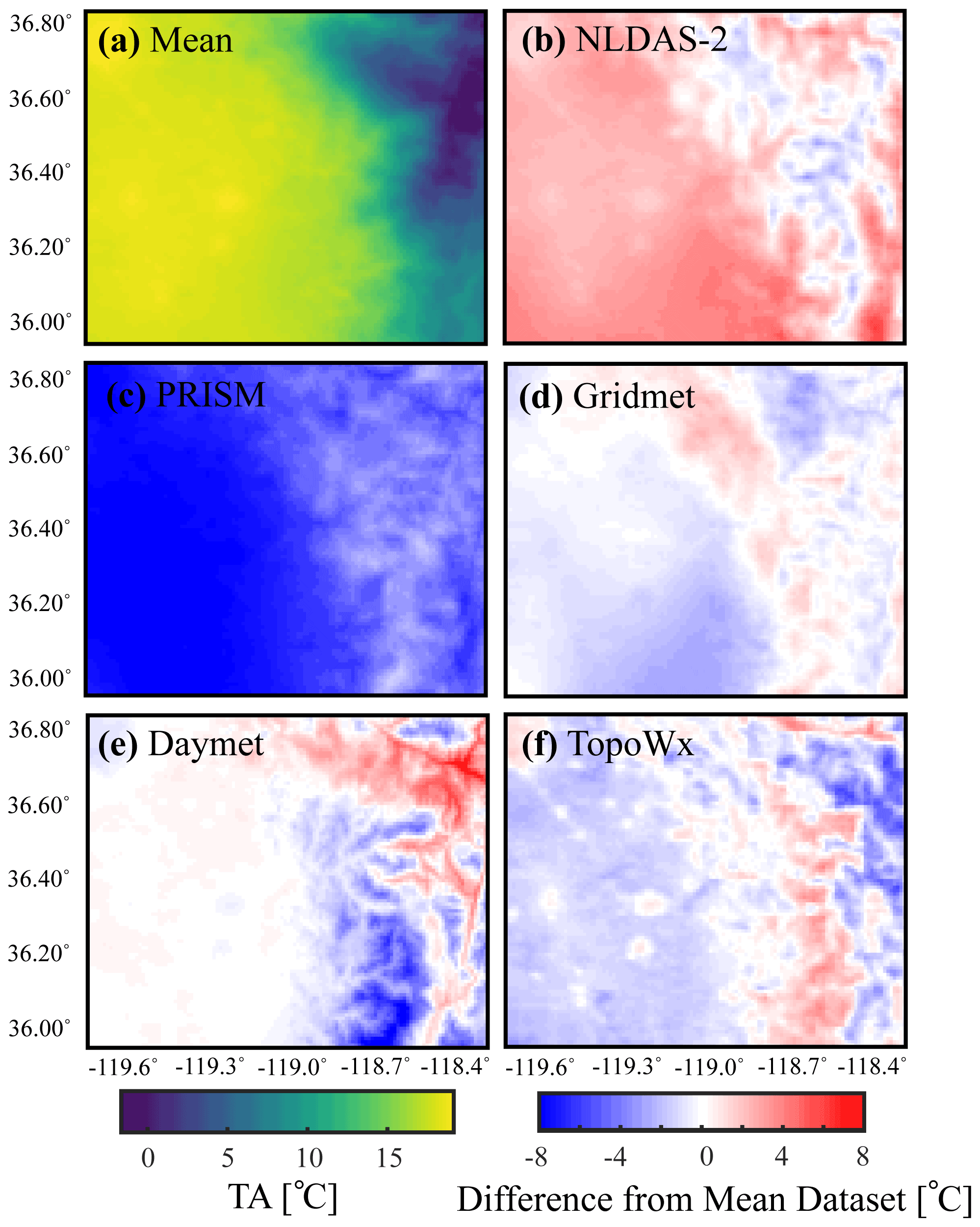
Figure 2 (a) Mean daily air temperature from five air temperature datasets used within this study for WY2016. Spatial maps represent differences in mean annual daily temperature from the mean dataset (calculated as dataset–mean) in (b) downscaled NLDAS-2, (c) PRISM, (d) Gridmet, (e) Daymet, and (f) TopoWx forcing datasets.

Model initialization consists of a two-step spin-up process to bring the subsurface water storage into dynamic equilibrium with the meteorological conditions. In the first step of the initialization, we start from a initially dry system and run the ParFlow code without the CLM by applying a constant-in-time net precipitation flux (P–ET) (Livneh et al., 2013) to fill up the groundwater storage and create a rough approximation of the flow network. From this point, each model scenario is run recursively using the ParFlow.CLM code and the WY2016 forcing data applied in that scenario (see scenario descriptions in Sect. 2.3). Recursive simulations are continued until the total subsurface storage reaches dynamic equilibrium (Ajami et al., 2014). We define dynamic equilibrium as the point at which the absolute change in total subsurface storage becomes less than 0.01 % in recursive simulations (Ajami et al., 2015). In addition to WY2016, we run simulations for WY2011 and WY2014 representing wet and dry conditions in the watershed, respectively (see Sect. 2.3). The model initialization process is repeated for each of these years using their respective meteorological forcings until the model reached dynamic equilibrium with respect to these forcings.

Model performance is extensively validated in Schreiner-McGraw and Ajami (2020). As we are focused on quantifying the impact of air temperature, we present a limited validation, using WY2016, primarily related to the energy budget. An important component of the land surface energy balance in mountainous terrain is the role of snow. We validate model performance using a reanalysis gridded product that contains estimates of snow water equivalent (SWE) and snow-covered area (SCA) for the majority of the Sierra Nevada (Margulis et al., 2016). This 90 m resolution dataset is generated using a Bayesian data assimilation technique with remotely sensed estimates of snow-covered area (Margulis et al., 2016). The dataset is clipped to 1500 m elevation to remove uncertainty related to the infrequent snow below this elevation. When making comparisons between this reanalysis dataset and our simulated datasets, we also set SWE and SCA below 1500 m elevation to 0. Additionally, we use remote sensing estimates of evapotranspiration (MOD16A2 product) at 1 km resolution from the MODIS Terra satellite to compare with simulated ET and test the performance of the simulated energy budget.

2.3 Model experiments

In this study, we are interested in quantifying how the uncertainty in air temperature and precipitation forcings impact the simulated water budget. To simplify the system and reduce the impact of uncertainty in anthropogenic management practices, we treat the system as a quasi-pre-development state that is not impacted by groundwater pumping, irrigation, or stream diversions. As a result, all of our model scenarios use consistent parameterizations for the subsurface and the land surface, and the only difference is in the air temperature and precipitation forcings from different gridded meteorological products. We perform a “base case” simulation where we use the mean precipitation from the four available datasets (Daymet, Gridmet, downscaled NLDAS-2, and PRISM) and the mean air temperature from the same four datasets plus the TopoWx dataset. Prior efforts have demonstrated that using the mean of the precipitation datasets results in the best model performance compared with simulations with each product individually (Schreiner-McGraw and Ajami, 2020). This base case scenario is used for comparison purposes. In addition to the base case scenario, we run three different numerical experiments: (1) variable precipitation and constant air temperature (VarPConstTA), (2) constant precipitation and variable air temperature (ConstPVarTA), and (3) variable precipitation and variable air temperature (VarPVarTA). In experiment 1, VarPConstTA, we run four scenarios each using the mean air temperature and one of the four precipitation datasets. Experiment 2 is the opposite with five scenarios, where each scenario is forced with the mean precipitation and one of the five air temperature datasets. Finally, experiment 3 consists of four scenarios, and each scenario is forced with the precipitation and air temperature from one of the four available gridded products. To assess how results are impacted by the choice of a single year of forcing data, we perform three numerical experiments for 3 different years, WY2011, WY2014, and WY2016, with above-average, below-average, and average precipitation totals, respectively. We focus our analysis on the year with near-average meteorological conditions (WY2016) and use the additional years to examine the variability and propagation of meteorological uncertainty introduced by unusually wet or dry conditions.

2.4 Analysis techniques

2.4.1 Relative importance of uncertainty in precipitation and air temperature for the simulated water budget

We first assess the uncertainty in the precipitation and air temperature datasets by calculating the mean absolute difference (MAD) between each pair of datasets at a daily scale for each grid cell in the domain (Henn et al., 2018). We calculate the MAD between a pair of datasets at a single grid cell as

$$\begin{array}{}\text{(1)}& {\text{MAD}}_{i,j}={\displaystyle \frac{\mathrm{1}}{d}}\sum _{k=\mathrm{1}}^d\mathrm{abs}\left(P_{i,k}-P_{j,k}\right),\end{array}$$

where i,j represents the difference between dataset i and dataset j, k represents the day, and d is the number of days in the year. We calculate the MAD for each pair of datasets and take the mean value of all MADs to represent the mean uncertainty in total precipitation for each year of forcing data. For presentation purposes, we also calculate the overall mean MAD using the 3 water years used in our simulations (WY2011, WY2014, and WY2016). The same approach is applied to air temperature. We acknowledge that this is not a true measure of uncertainty in precipitation or air temperature as ground truth data from weather stations are not available.

Next, we assess the relative importance of uncertainty in the precipitation and air temperature forcing datasets for the annual water budget partitioning from each simulation scenario. We perform this calculation for the Kaweah Terminus watershed, upstream of the Terminus dam (Fig. 1), to focus on the mountain groundwater system. The Terminus dam is not represented in the model, and streamflow evaluation downstream of this point is difficult. We calculate the groundwater flux (GW) out of the Kaweah Terminus watershed as a residual of the annual water balance, $\text{GW}=P-\text{ET}-Q-\mathrm{d}S$, where P is the precipitation, ET is the evapotranspiration, Q is the streamflow, and dS is the change in subsurface storage. This groundwater flux is equivalent to the mountain block recharge (MBR) that is generated within the Kaweah Terminus watershed. We additionally calculate the precipitation partitioning into rain and snow components. The version of the CLM in the model uses a threshold air temperature of 2.5 ^∘C to partition precipitation, so we apply the same threshold to the precipitation data to determine snowfall and rainfall.

Given the seasonality of the water balance in the study watershed, we also calculate the monthly relative range of hydrologic fluxes from the Kaweah Terminus watershed to determine months with the highest uncertainty in simulated fluxes. The relative range (R_r) is defined as the range in monthly simulated hydrologic fluxes for each experiment divided by the monthly value from the base case scenario.

2.4.2 Relative elasticity and sensitivity metrics to changes in precipitation and air temperature

To determine the relative sensitivity of the simulated annual hydrologic budget to precipitation and air temperature forcings, we calculate the sensitivity and elasticity of multiple hydrologic variables relative to the baseline simulation for the Kaweah River watershed (Fig. 1). We perform these calculations using the catchment-averaged values from experiment 1 (P elasticity) and experiment 2 (T_air sensitivity) simulations where P and T_air are modified individually. The precipitation elasticity (ε) is the fractional change in a hydrologic variable v from dataset i divided by the fractional change in P from dataset i, both relative to our base case scenario.

$$\begin{array}{}\text{(2)}& \mathit{\epsilon }={\displaystyle \frac{\frac{v_i-v_{\text{base}}}{v_{\text{base}}}}{\frac{P_i-P_{\text{base}}}{P_{\text{base}}}}}\end{array}$$

Following the reasoning from Vano et al. (2012), we also calculate the temperature sensitivity (S) in a similar manner. We define S as the percent change in a hydrologic variable v, caused by a change in T_air.

$$\begin{array}{}\text{(3)}& S={\displaystyle \frac{\frac{v_i-v_{\text{base}}}{v_{\text{base}}}}{T_{{\text{air}}_i}-T_{{\text{air}}_{\text{base}}}}}\end{array}$$

While we cannot directly compare whether T_air or P uncertainty adds more variability to hydrologic simulations, by comparing the ε and S, we can determine whether the range of uncertainty in T_air or P contained in common gridded datasets adds more uncertainty to the simulated hydrologic budget. We recognize that the ε and S are overestimated in this analysis because the datasets have different spatial patterns in T_air and P, and the basin average differences in simulated hydrology are not solely caused by the basin average differences in T_air and P. We contend, however, that this is a reliable approach to estimate the relative importance of model forcing dataset selection. We also assess spatial variability of precipitation elasticities and temperature sensitives by applying Eqs. (2) and (3) at the pixel scale.

2.4.3 Impact of combined uncertainty in precipitation and air temperature on the simulated water budget

As a result of climate change, both P and T_air are expected to change simultaneously. In the analysis described above, we only alter P or T_air individually in experiments 1 and 2, respectively. We make use of the scenarios from experiments 1, 2, and 3 to examine the combination effects of uncertainty in both P and T_air on simulated hydrologic response in the Kaweah River watershed for each simulated water year. We calculate the relative change in a hydrologic variable, v, relative to our “base case” scenario forced with the mean of both the air temperature and precipitation datasets. For each forcing dataset (Daymet, Gridmet, etc.), we calculate the individual relative difference in simulated hydrologic fluxes or states caused by changing the precipitation dataset (v_ΔP) and the temperature dataset ($v_{\mathrm{\Delta }{T}_{\text{air}}}$) from the base case using catchment-averaged values. We then estimate the total relative differences in simulated hydrology caused by the combined changes in P and T_air by summing the relative differences of P and T_air as if there were no interaction effects ($v_{\mathrm{\Delta }P\mathrm{\Delta }{T}_{{\text{air}}_{\text{est}}}})$ (Vano et al., 2012):

$$\begin{array}{}\text{(4)}& v_{\mathrm{\Delta }P\mathrm{\Delta }{T}_{{\text{air}}_{\text{est}}}}={\displaystyle \frac{\left(v_{\mathrm{\Delta }P}-v_{\text{base}}\right)}{v_{\text{base}}}}+{\displaystyle \frac{\left(v_{\mathrm{\Delta }{T}_{\text{air}}}-v_{\text{base}}\right)}{v_{\text{base}}}}.\end{array}$$

The estimated combined impact of P and T_air changes on the variable, v, are then compared with the simulated values of a given variable when both P and T_air are simultaneously altered in model simulations ($v_{\mathrm{\Delta }P\mathrm{\Delta }{T}_{\text{air}}}$) to determine the degree of interaction effects for both variables in the Kaweah River watershed.

2.4.4 Sensitivity of recharge pathways to meteorological forcings

We make use of the integrated hydrologic model to examine the sensitivity of different recharge pathways to changes in P and T_air forcing. We calculate recharge via three primary pathways, MAR (derived from rain or snow), MBR, and MFR. We calculate each of these fluxes using the simulated pressure head and saturation values and the Richards equation (Maxwell and Miller, 2005) for specific regions of the model domain. MAR is defined as the vertical flux of water leaving the 2 m-deep soil zone (potential recharge) within the Kaweah Terminus watershed, located upstream of the Terminus dam in the Sierra Nevada (Fig. 1). We separate MAR derived from snowmelt as MAR that occurs in the same model time step that snowmelt occurs (i.e., changes in daily SWE is negative), and otherwise we assume that MAR is sourced from rainfall. We estimate the MBR sourced from the mountainous region of the Kaweah Terminus watershed as a residual of the water balance that is equivalent to the GW flux out of the watershed. We recognize that this is not explicitly MBR because the Kaweah Terminus boundary does not exactly trace the boundary between the mountain block and the valley aquifer. However, the regional flow pathways ensure that groundwater leaving the Terminus watershed will reach the Central Valley aquifer. Finally, MFR is calculated as the volume of streamflow that infiltrates into the channel bottom as the Kaweah River flows across the piedmont slope, defined as the area adjacent to the mountain block where topographic slope is greater than 2 % (11 km of the Kaweah River reach).

Previous efforts have shown the role of topography in the propagation of uncertainty in precipitation to groundwater (Schreiner-McGraw and Ajami, 2020). To examine how this propagation impacts MAR under the combined P and T_air uncertainty versus individual uncertainty in P or T_air, we make use of the relationship between the topographic wetness index (TWI) and uncertainty in simulated MAR, where the TWI is calculated as

$$\begin{array}{}\text{(5)}& \text{TWI}=\ln \left({\displaystyle \frac{A_{\text{C}}}{\tan \mathit{\alpha }}}\right),\end{array}$$

where A_C is the contributing drainage area and α is the slope (Beven and Kirkby, 1979). As the TWI is meant to be applied in climatically similar regions, we apply the analysis only to the Kaweah Terminus watershed where land cover and subsurface geology are constant, and climate is relatively similar (mean annual precipitation ranges from 435 to 960 mm yr⁻¹ and mean annual T_air ranges from 0 to 15 ^∘C). We estimate the uncertainty in the simulated MAR as the standard deviation of MAR values from the multiple scenarios in each TWI bin.

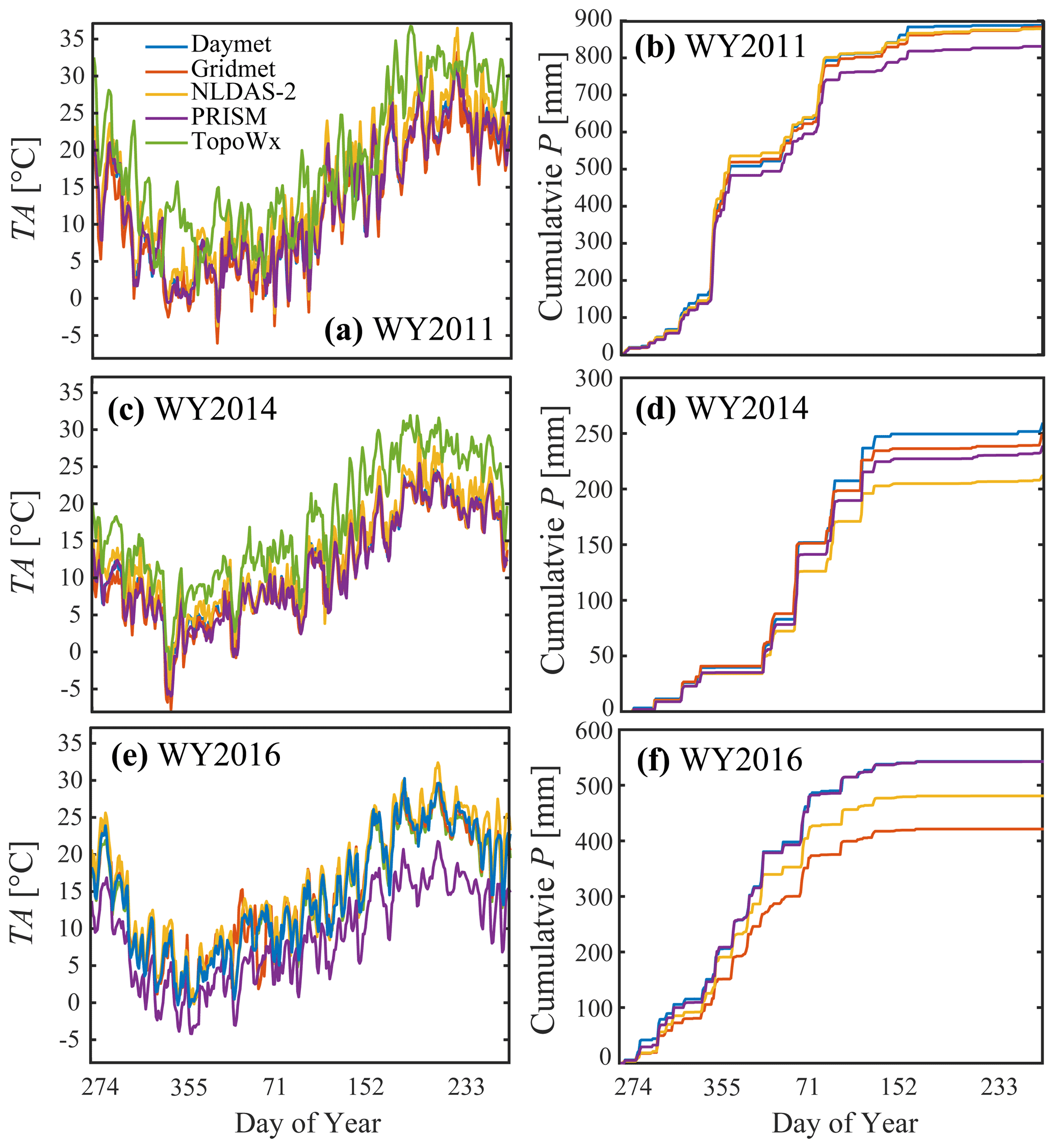
Figure 3 (a, c, e) Daily domain-averaged values of air temperature for five temperature datasets and (b, d, f) the cumulative sum of domain-averaged precipitation for each of the four gridded datasets in (a, b) WY2011, (c, d) WY2014, and (e, f) WY2016.

3 Results and discussion

3.1 Air temperature and precipitation uncertainty

Differences in mean annual daily temperature from the mean temperature dataset range between −8 and 8 ^∘C (Fig. 2b–f). Differences in mean daily temperature among different forcing datasets exist irrespective of the wetness condition (wet vs. dry or average year), and the ranges are larger for WY2011 (Fig. 3a, c, e). Considerable uncertainty exists in the daily and annual totals of precipitation from the different gridded datasets as well (Fig. 3b, d, f). The differences between the gridded products in our study are surprising, especially considering that Gridmet is based on the NLDAS-2 and PRISM datasets. We believe that the differences among products are caused by contrasting spatial resolutions. For example, Abatzoglou (2013) used the 800 m PRISM data to generate the Gridmet dataset, while we used the freely available PRISM data at 4 km resolution. Additionally, we used a downscaled version of the NLDAS-2 dataset called the Princeton CONUS Forcing dataset at ∼3 km resolution with the updated precipitation data using the Stage IV and Stage II radar products. We believe that the differences in the resolution of the datasets and interpolation approaches have caused the differences in precipitation and air temperature forcing datasets.

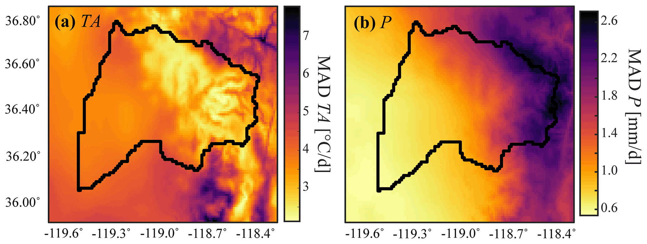
Figure 4 Uncertainty in the daily air temperature (a) and precipitation (b) datasets represented by the mean absolute difference (MAD) for the 3 water years (2011, 2014, and 2016) used in this study.

We analyze the uncertainty in the forcing datasets by presenting the average MAD between the datasets available for T_air (Fig. 4a) and P (Fig. 4b) for 3 water years. Figure 4a presents the annual mean daily MAD averaged across the five temperature datasets and 3 water years. Overall, the uncertainty in air temperature is high, with large portions of the model domain expressing an average MAD of greater than 5^∘ d⁻¹. The MAD in the topographically flat portion of the domain in the Central Valley is relatively consistent, with values of approximately 4^∘ d⁻¹. The mountainous region of the study domain has more variability in temperature-based MAD estimates. Coincidentally, the majority of the mountainous portion of the Kaweah River watershed has a relatively low MAD in T_air, and mountainous regions outside the watershed boundary have a much higher uncertainty in T_air that in places exceeds 7^∘ d⁻¹. Uncertainty in P follows a more consistent pattern than uncertainty in T_air, where the MAD in P increases consistently with elevation (Fig. 4b). This pattern is partially attributable to the annual total precipitation increases in the high-elevation regions, but the lack of meteorological gauges at high elevations also increases the uncertainty in these regions. The spatial patterns of the MAD for both P and T_air remain relatively constant between years, suggesting that the differences are related to the interpolation algorithms rather than different observed data. These findings are consistent with previous efforts to quantify uncertainty in gridded precipitation datasets that found uncertainty between 150 and 200 mm yr⁻¹ in this region (Henn et al., 2018; Lundquist et al., 2015).

Figure 5 Monthly ET in WY2016 from the MODIS remote sensing product (solid lines) as well as the range of simulated ET from each of the three experiments (a) VarPConstTA, (b) ConstPVarTA, and (c) VarPVarTA (dashed lines) in the Kaweah River watershed. Croplands are removed from this comparison as irrigation is not included in simulations.

3.2 Model validation

A comprehensive validation of model performance is presented in Schreiner-McGraw and Ajami (2020). In this study we present a validation of model performance in simulating two components of the energy balance, ET and SWE, using WY2016 simulations. Figure 5 presents a comparison between the simulated ET from each of the experiments 1, 2, and 3 and remote sensing values from the 8 d MODIS product. The values presented are watershed average values for the Kaweah River watershed with irrigated croplands removed due to the lack of irrigation in the simulations. Generally, the range of simulated monthly ET encompasses the remote sensing values. The peak value of monthly ET of 40 mm month⁻¹ is replicated by the model simulations. The timing of the peak value, however, is inconsistent between the simulations and the remote sensing product. At the monthly scale, both the peak ET and the minimum ET throughout the year are delayed by 1 month. This result is partially attributable to the coarse temporal resolution of the remote sensing data composited at 8 d intervals as well as the monthly aggregation of these data. In addition, we believe that some of the discrepancy arises from restricting the plant rooting depth in the simulations to the top 2 m of soil in ParFlow.CLM simulations, limiting their ability to draw on water stored in the saprolite layer. As saprolite storage is recharged by spring snowmelt (Thayer et al., 2018), this model specification creates temporal discrepancy in ET. Because the simulated energy budget captures ET quantities, however, we are satisfied with the model performance considering the study objectives. The patterns observed during WY2016 are replicated in WY2011 and WY2014, but the peak simulated ET is delayed relative to the remote sensing product. For the rest of the year, the remotely sensed values are generally bracketed by the range of simulated ET values.

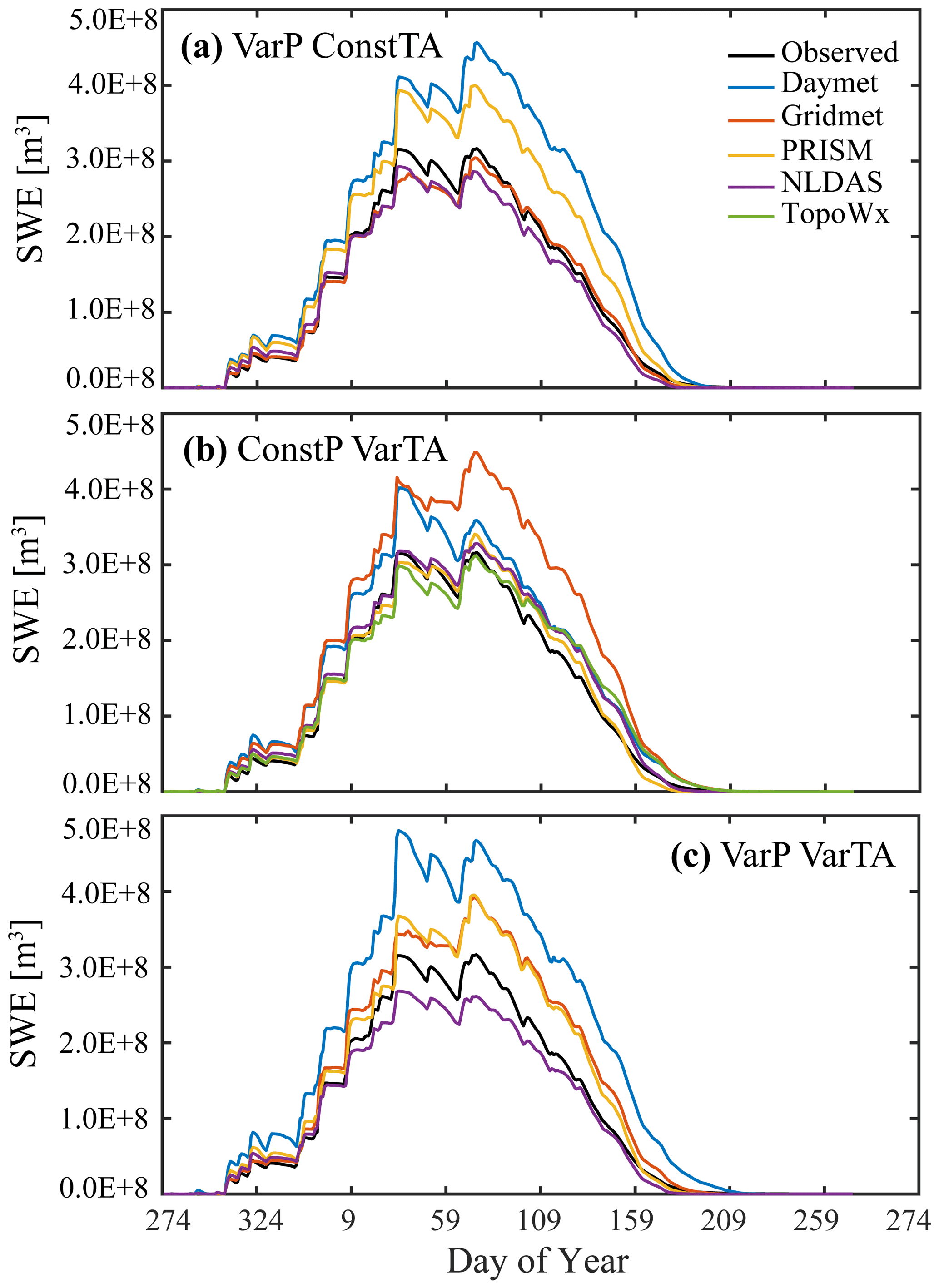
Figure 6 Daily SWE from the reanalysis product (black lines) as well as the range of simulated SWE from each of the three experiments (a) VarPConstTA, (b) ConstPVarTA, and (c) VarPVarTA (color lines) in WY2016.

We also assess the performance of the energy budget simulations by comparing the simulated SWE with a reanalysis product developed for the Sierra Nevada region (Margulis et al., 2016) using the WY2016 simulations. Figure 6 presents the annual cycle of snowpack accumulation and melting as simulated SWE from each of the three experiments. We present the total volume of SWE for each day in the Kaweah River watershed. For all the experiments, the simulated annual pattern of daily SWE encompasses the observed values. The only exception is the period from DOY 65 to 150 from the ConstPVarTA scenarios, where the simulated SWE is larger than the reanalysis product values (Fig. 6b). In the ConstPVarTA scenarios, significant variability within the simulated SWE exists, especially for the peak SWE values. The peak SWE of the Daymet scenario is 27 % higher than that observed, and SWE from the Gridmet scenario is 42 % higher than that observed. The Daymet and Gridmet datasets have lower air temperatures in the mid-elevation zone, where temperatures fluctuate between below and above freezing (Fig. 2). In terms of timing, the peak SWE occurs on DOY 74 for all ConstPVarTA scenarios, except in the Daymet forcing scenario, where the peak SWE occurs on DOY 34. The timing of full snowmelt is more variable and is delayed for the scenarios with higher peak SWE. Full snowmelt occurs on DOY 216 for Daymet, DOY 221 for Gridmet, DOY 211 for downscaled NLDAS-2, and DOY 194 for the PRISM scenario. The simulated SWE from each of the VarPConstTA scenarios (Fig. 5a) has similar temporal patterns, but there is considerable spread in the SWE values that reflects the spread in precipitation volumes from the different forcing datasets. The VarPVarTA scenarios have the largest variability in SWE across the forcing datasets, with downscaled NLDAS-2 forcing underestimating the peak SWE and other forcings overestimating it relative to the observations (Fig. 6c). In WY2011 and WY2014, as in WY2016, the observed SWE is bracketed by the range of simulated values.

3.3 Recharge pathway sensitivity to meteorological variability

Mountain system recharge to the Central Valley is a key unknown for water management in this highly productive agricultural system. During WY2016, with roughly average meteorological conditions, the total mountain system recharge from the mountainous portion of the Kaweah River watershed, the Kaweah Terminus sub-watershed, to the valley aquifer (MBR + MFR) ranges from 186 to 504 mm yr⁻¹, depending on which meteorological forcing scenario is used. In our simulations, the majority of this recharge comes from the MFR pathway, and the ratio of MFR $/$ (MBR + MFR) ranges from 0.85 to 0.99 across all simulations performed. Our results are consistent with observational studies (Visser et al., 2018), but there is considerable uncertainty related to characterizing the source of mountain system recharge.

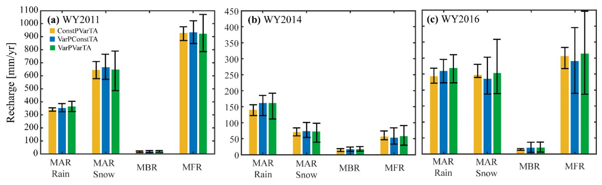
Figure 7 Mean and standard deviation of simulated mean MAR from rain and snow, mountain block recharge (MBR), and mountain front recharge (MFR) from scenarios in three simulation experiments: ConstPVarTA, VarPConstTA, and VarPVarTA in the Kaweah Terminus watershed. Results are presented for WY2011 (a), WY2014 (b), and WY2016 (c).

Across all simulations, the total MAR (MAR from rain + MAR from snow) is dramatically larger than the MBR. This is expected as the MAR is calculated as the potential recharge, and most of it may flow via local flow paths to topographically convergent zones, where it could be subsequently transpired or discharged as baseflow, while the remainder becomes MBR. Figure 7 presents the range of simulated annual recharge from each of the mountain system recharge pathways for each year of equilibrium simulations. For all recharge pathways, the simulated value is impacted by the choice of temperature and precipitation datasets. Using the average conditions in WY2016 as an example, the temperature datasets used in the ConstPVarTA scenarios result in a range of simulated recharge that is 16 %, 24 %, 3 %, and 24 % of the mean value from the five scenarios for the MAR from rain, MAR from snow, MBR, and MFR pathways, respectively. The corresponding precipitation datasets included in the VarPConstTA scenarios result in a larger range in simulated recharge for all recharge pathways. The range of simulated recharge for the VarPConstTA scenarios is 26 %, 52 %, 240 %, and 76 % of the mean of the four scenarios for the MAR from the rain, MAR from snow, MBR, and MFR pathways, respectively. When variability in T_air is added to P variability in the VarPVarTA scenarios, the range of simulated recharge for each pathway increases to 33 %, 70 %, 238 %, and 91 % of the mean of the four VarPVarTA scenarios, for the MAR from rain, MAR from snow, MBR, and MFR pathways, respectively. While the magnitudes of various recharge pathways are different during the wet (WY2011) and dry (WY2014) years compared with WY2016 simulations, the WY2016 patterns are replicated in all 3 simulation years (Fig. 7).

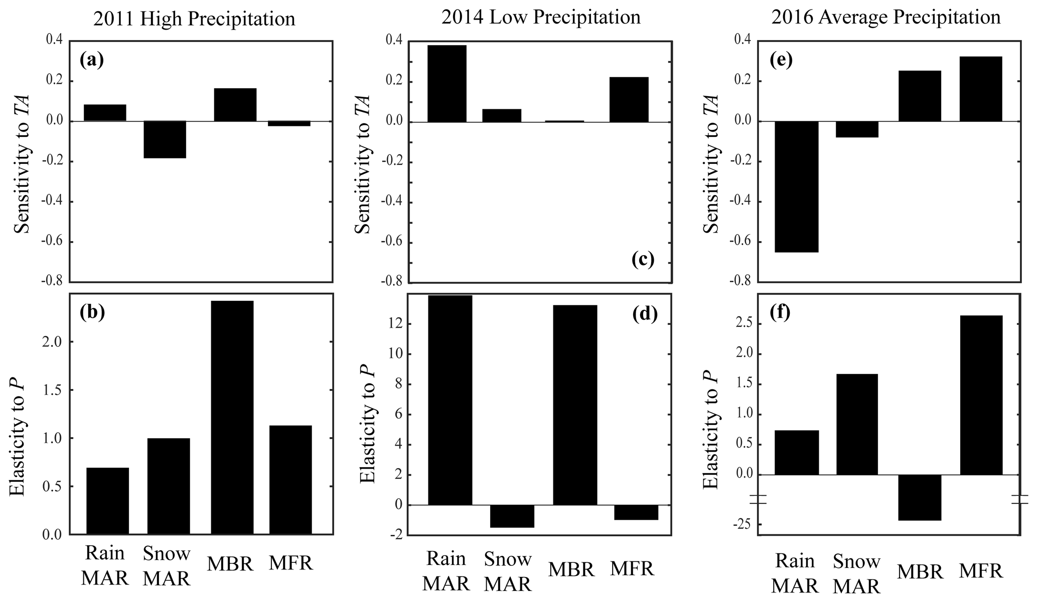
Figure 8 Sensitivity to T_air and elasticity to P of different mountain system recharge pathways for WY2011 (a, b), WY2014 (c, d), and WY2016 (e, f). Each bar represents the mean value for the scenarios in the ConstPVarTA (a, c, e) and VarPConstTA (b, d, f) experiments in the Kaweah Terminus watershed.

To compare the sensitivity of each mountain recharge pathway with changes in meteorological forcings, we calculate the ε and S for different recharge pathways in the Kaweah Terminus watershed. Figure 8 displays the average ε and S across the four forcing datasets for each of the four mountain recharge pathways in each year of equilibrium simulation. During the average conditions in WY2016 and the wet year of WY2011, MBR and MFR are more sensitive to the precipitation datasets than the MAR components. While the rain MAR is the most sensitive pathway to changes in T_air datasets under average conditions, the sensitivity of snow MAR is highest under wet conditions. During low-precipitation conditions (WY2014), the rain MAR is highly sensitive to changes in both T_air and P compared with other recharge pathways due to extreme water limitation and the small magnitude of recharge from soils. For all 3 simulated years, the snow MAR expresses low sensitivity to the T_air datasets ($\left|S\right|<\mathrm{0.2}$). This result in part is a reflection of the higher mean snow MAR values that make changes relative to the mean value smaller. Additionally, most of the precipitation uncertainty is in the high-elevation zone where temperatures are low across all forcing datasets and snow is dominant. As a result, although we might expect snow MAR to be highly sensitive to changes in T_air, it is more sensitive to changes in P. Following the same logic, each of the three recharge pathways that is controlled by SWE (snow-derived MAR, MBR, and MFR) is more sensitive to changes in P than changes in T_air (Fig. 8). Much higher ε values than the S values during the dry and wet years indicate that the recharge pathways are more sensitive to changes in the P dataset than the T_air dataset even during the high-precipitation year (WY2011), which is a result of the water-limited conditions in California.

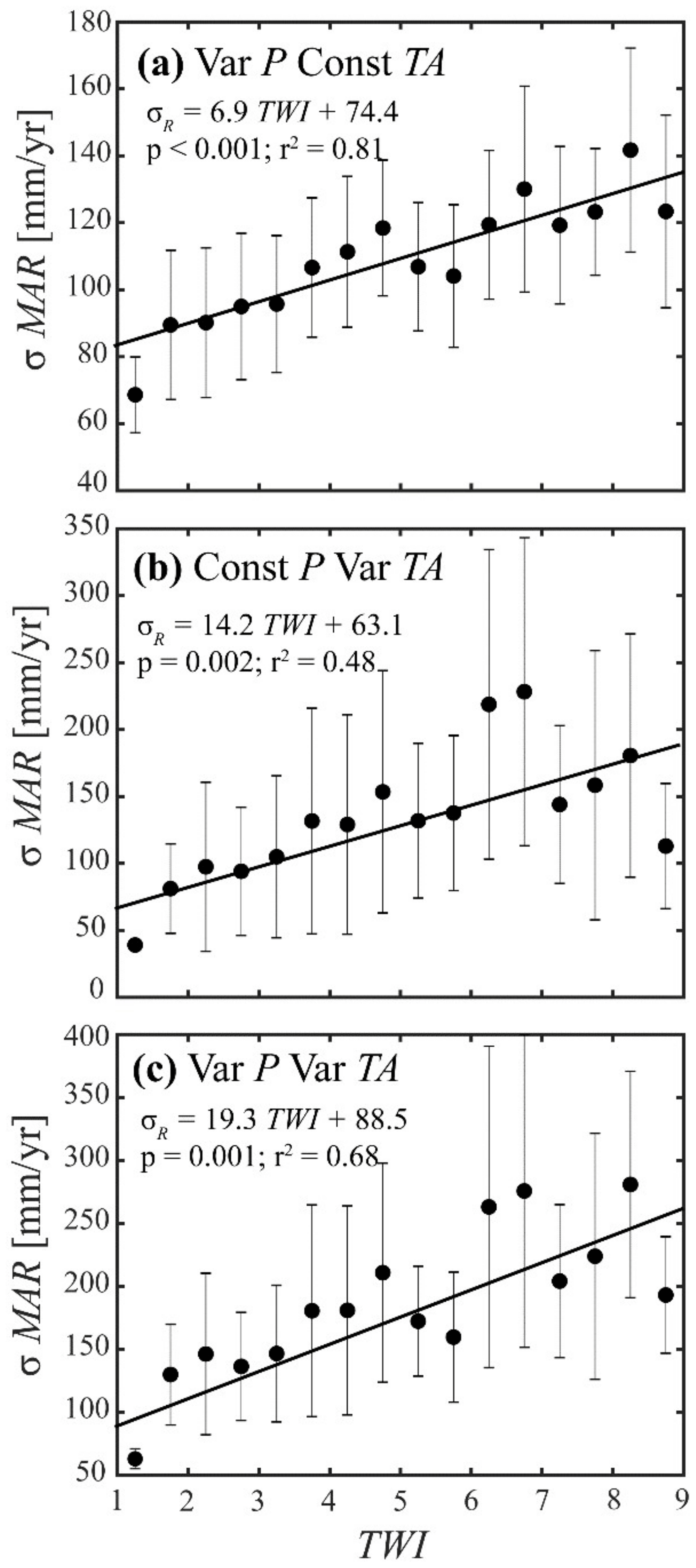
Figure 9 Scatterplots between the binned values of TWI and the standard deviation of MAR from each of the scenarios included in the WY2016 VarPConstTA experiment (a), the ConstPVarTA experiment (b), and the VarPVarTA experiment (c) in the Kaweah Terminus watershed. Circles represent the bin average, and the bars represent the bin's standard deviation. Solid lines present statistically significant (p<0.05) linear regressions.

Prior efforts have demonstrated that topography-driven subsurface flow is an important process that redistributes uncertainty in P forcing throughout the watershed (Schreiner-McGraw and Ajami, 2020). Figure 9 presents the relations between TWI and the uncertainty in simulated MAR (σMAR – defined as the standard deviation of recharge across the scenarios in each experiment) for the Kaweah Terminus watershed in WY2016. We limit this analysis to the Kaweah Terminus watershed because it has the same vegetation type (evergreen forest) and relatively consistent climate conditions to make the TWI a valid expression of the topographic effect on soil water movement. By limiting the analysis to the mountainous region, the potential recharge is equivalent to our definition of MAR. Across all the experiments, the uncertainty in MAR increases with TWI because topography-driven flow moves water into convergent zones via lateral soil and shallow groundwater fluxes. An ANCOVA test reveals that the strength of the topographic control in MAR uncertainty is higher for the ConstPVarTA scenarios than the VarPConstTA scenarios, as represented by the statistically significant higher slope (Fig. 9a and b). This result, along with higher soil moisture values (data not shown), suggests that the ET in convergent zones is more energy limited than water limited throughout the year, so T_air uncertainty creates larger variability in ET than P uncertainty. Supporting this idea, the patterns are replicated in the WY2011 and WY2014 datasets as well. Due to the link between ET and potential recharge via soil wetness, the variability in ET is reflected in increases in MAR variability. When uncertainty in both T_air and P is considered, the slope of the TWI and σMAR relation increases, but according to an ANCOVA test, the slope is not significantly different (p<0.05) than the ConstPVarTA scenarios. The relations between TWI and σMAR are consistent in WY2011 and WY2014 with WY2016, and the VarPVarTA scenarios have a higher slope, but it is not significantly different (p<0.05). Because topography-driven subsurface flow concentrates soil water in convergent zones, the individual spatial patterns of P and T_air uncertainty become less important, and their uncertainties cancel each other out, creating consistently negative interaction effects in the VarPVarTA scenarios. This impact is more pronounced with MAR compared with other variables because MAR is the most dependent variable on topography-driven flow.

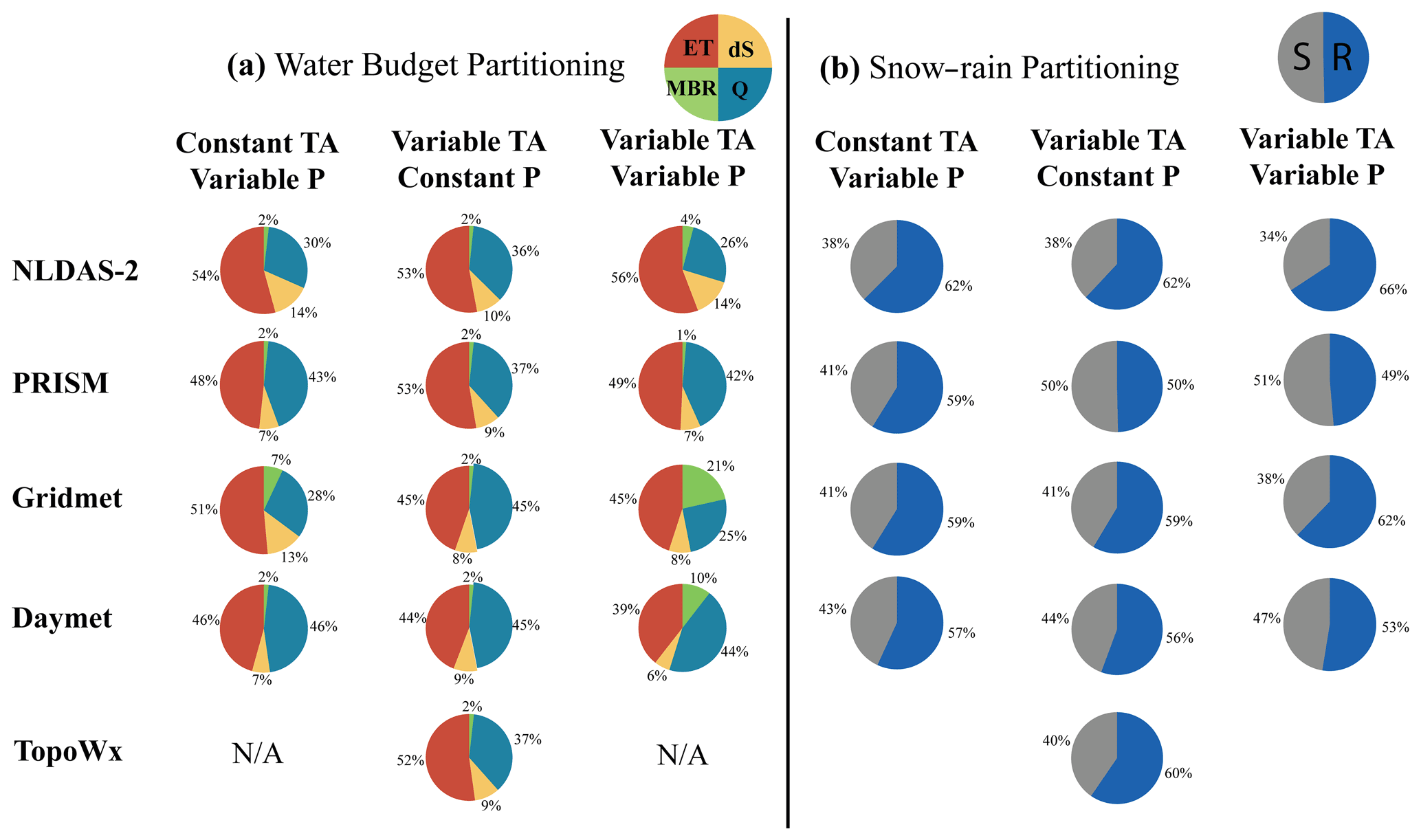
Figure 10 (a) Water budget partitioning shown as a fraction of the incoming annual precipitation for the Kaweah Terminus watershed during WY2016 and (b) rain–snow partitioning in the Kaweah Terminus watershed for each of the scenarios in the three simulation experiments during WY2016. Fractions are rounded to the nearest 1 %.

3.4 Relative importance of precipitation and air temperature uncertainty for the simulated water budget

To address research question 2, whether uncertainty in P or T_air data impacts the simulated hydrology of a mountain watershed, we plot the annual water budget partitioning for WY2016 with average meteorological conditions. Figure 10a presents the simulated annual water budget partitioning for the mountainous Kaweah Terminus watershed for all of the scenarios in experiments 1, 2, and 3 for WY2016. The Kaweah Terminus watershed is used because it is the largest sub-watershed in the domain where accurate streamflow simulations can be ensured through model validation. Variable precipitation forcing applied in experiment 1 (VarPConstTA) results in significant changes to the water budget partitioning. For all P forcing datasets (ConstTAVarP scenarios), MBR remains the smallest portion of the water budget, while ET comprises the largest portion of the water budget. The largest changes in the water budget partitioning occur in the simulated Q that ranges from 28 % to 46 % of the precipitation. Changes to the T_air forcing dataset when the precipitation is constant (ConstPVarTA scenarios) result in similar patterns to changes to the P forcing when the temperature is constant. For all T_air datasets, ET is the largest component of the water budget and MBR is the smallest. The variable T_air scenarios result in a smaller range of simulated Q (36 %–45 %) than the variable P datasets (28 %–46 %) but a larger range in simulated ET (46 %–54 % for VarPConstTA and 44 %–53 % for ConstPVarTA). The right-most column in Fig. 10a presents the water budget partitioning when both T_air and P forcing datasets are varied. There is considerable uncertainty in the major water budget components, and when both Daymet P and T_air are used, the water budget shifts so that ET is no longer the largest component. The ET ranges from 39 % (Daymet) to 56 % (downscaled NLDAS-2), while Q ranges from 25 % (Gridmet) to 44 % (Daymet) of the total water budget. These ranges are much larger than the range in water budget partitioning caused by modifying P or T_air individually and suggest that the uncertainty from the individual forcing variables is additive rather than cancelling each other out. Besides P and T_air uncertainties, differences in the water budget partitioning of VarPVarTA scenarios are due to nonlinear feedbacks between the spatial patterns of P and T_air and subsurface properties, vegetation type, and topography. Although the proportion of P that becomes ET and Q varies depending on the annual precipitation amount, this pattern in water budget partitioning remains consistent with WY2011 and WY2014 as well.

To explain the simulated water budget partitioning during WY2016, Fig. 10b presents the proportion of the total precipitation that falls as snow or rain for each scenario from experiments 1, 2, and 3. Changes to the T_air forcing dataset create a larger range in the snowfall $/$ P ratio than changes to the P forcing dataset (snowfall $/$ P ratios of 38 %–43 % in VarPConstTA and 38 %–50 % in VarTAConstP). A close inspection of the charts presented in Fig. 10 suggests that the snow $/$ rain ratio impacts the annual water budget partitioning, and Fig. 10a–c demonstrate this conclusion by presenting relations between the ratio of snowfall $/$ P and the ET $/$ P, MBR $/$ P, and $Q/P$ ratios. Each point in Fig. 11 represents the mean value for each scenario in experiments 1, 2, and 3 for WY2016. Statistically significant linear relations (p<0.05) demonstrate that an increase in the proportion of P that falls as snow decreases the ET $/$ P ratio and increases the $Q/P$ ratio. As the ConstPVarTA scenarios create a larger range in the snowfall $/$ P ratio than the VarPConstTA scenarios (Fig. 10b), this raises the question of why the ConstPVarTA scenarios do not create a larger range in simulated MBR or Q. Although there are significant relations (p<0.05) between the snowfall $/$ P ratio and water budget partitioning, the relations are weak, with r² values between 0.17 and 0.35. Figure 11d–f present the relations between the total annual snowmelt (S_m) and the ET $/$ P, MBR $/$ P, and $Q/P$ ratios. The S_m has stronger relations to the water budget partitioning than the snowfall $/$ P ratio, with r² values of 0.68–0.79. In the mountainous study watershed, the total volume of snowmelt is more dependent on P than T_air because the high-elevation regions where the majority of the precipitation falls remain below freezing for most of the wet season across all the air temperature datasets. The increased variability in total snowmelt results in the larger changes to Q and MBR caused by the VarPConstTA scenarios.

In the Mediterranean climate of California, the distinct dry season creates challenges for water management, making the temporal patterns in simulated water budget variability of interest. Figure 12 presents the monthly time series of ET, MAR, and Q from the Terminus watershed for the base case scenario (solid lines) with the range of simulated values (dashed lines) as well as the relative range for each (black bars) during WY2016. The variable P forcings, from the VarPConstTA scenarios, result in a relatively consistent monthly ET-based R_r throughout the year. On average, the ET-based R_r is 0.2 throughout the year, and January (0.3) and February (0.1) are the months with the largest discrepancies. Changes in the P forcing dataset cause larger variability in the R_r for the Q and MAR, but a seasonal pattern does not emerge. Scenarios with altered T_air, however, display a more prominent annual trend in the R_r of simulated ET and Q. The ET-based R_r is considerably higher in November, December, and January for the ConstPVarTA scenarios (average R_r is 0.5) compared with 0.07 for the rest of the year. This increase in ET-based R_r during the winter months of the ConstPVarTA scenarios is consistent across all 3 simulation years. This finding is striking because the divergence in the T_air forcing datasets is primarily found during the summer months (DOY ∼150–230) (Fig. 3). We attribute this result to the fact that ET does not occur if the temperatures are below freezing, and T_air variability at a given location may result in below-freezing temperature for one T_air dataset but not another. The Q-based R_r increases during March through July are consistent with the snowmelt period and increases in T_air variability (Fig. 3). During the dry WY2014, the Q-based R_r increases between March and May as the lower snowpack shortens the snowmelt period when streamflow is high. For the wet WY2011, the Q-based R_r remains high through August as the wetter conditions result in more streamflow throughout the summer period. For VarPVarTA experiments, in all 3 years, the MAR-based R_r varies throughout the year without consistent patterns emerging.

3.5 Sensitivity and elasticity of the simulated water budget to precipitation or air temperature

To determine the relative sensitivity of the simulated annual hydrologic budget to precipitation and air temperature forcings, we present the elasticity (ε) and sensitivity (S) of water budget components to changes in P or T_air, respectively. Figure 13 presents the ε and S calculated for each meteorological forcing scenario in experiments 1 and 2, relative to the base case, for the water budget components simulated using the average WY2016 conditions. In general, results suggest that the water budget is very sensitive to changes in forcing. Elasticities are larger than 1 for most datasets, and variables such as SWE, dS, potential recharge (R), and Q at the Terminus dam indicate that the simulated variables exhibit a larger percent change than the percent change in precipitation. The sensitivity of the simulated water budget to changes in temperature is also quite high, especially when the Gridmet and downscaled NLDAS-2 datasets are used (Fig. 13b). The only hydrologic variables that are not heavily impacted by changes in P or T_air are the land surface temperature (T_g) and root zone volumetric water content (θ). At the annual scale, the result of θ is not surprising because the soil moisture is controlled by both ET and R, where an increase in one can be compensated for by a decrease in the other flux. Additionally, variability of these fluxes is highest at a daily compared with annual scale. We believe that lower sensitivity of T_g is related to the simplification made to represent the ground heat flux calculation in the CLM. To reduce computational time, many land surface models, including the CLM, only incorporate heat transport via conduction, and this simplification decouples heat transport from soil moisture transport (Kollet et al., 2009). Overall, the water budget exhibits high ε and S to both changes in P and T_air. This behavior does not necessarily mean that the magnitudes of P and T_air effects on the water budget are equal. It means that the range of uncertainty contained in the meteorological forcing datasets for both P and T_air results in similar amounts of uncertainty in the simulated water budget.

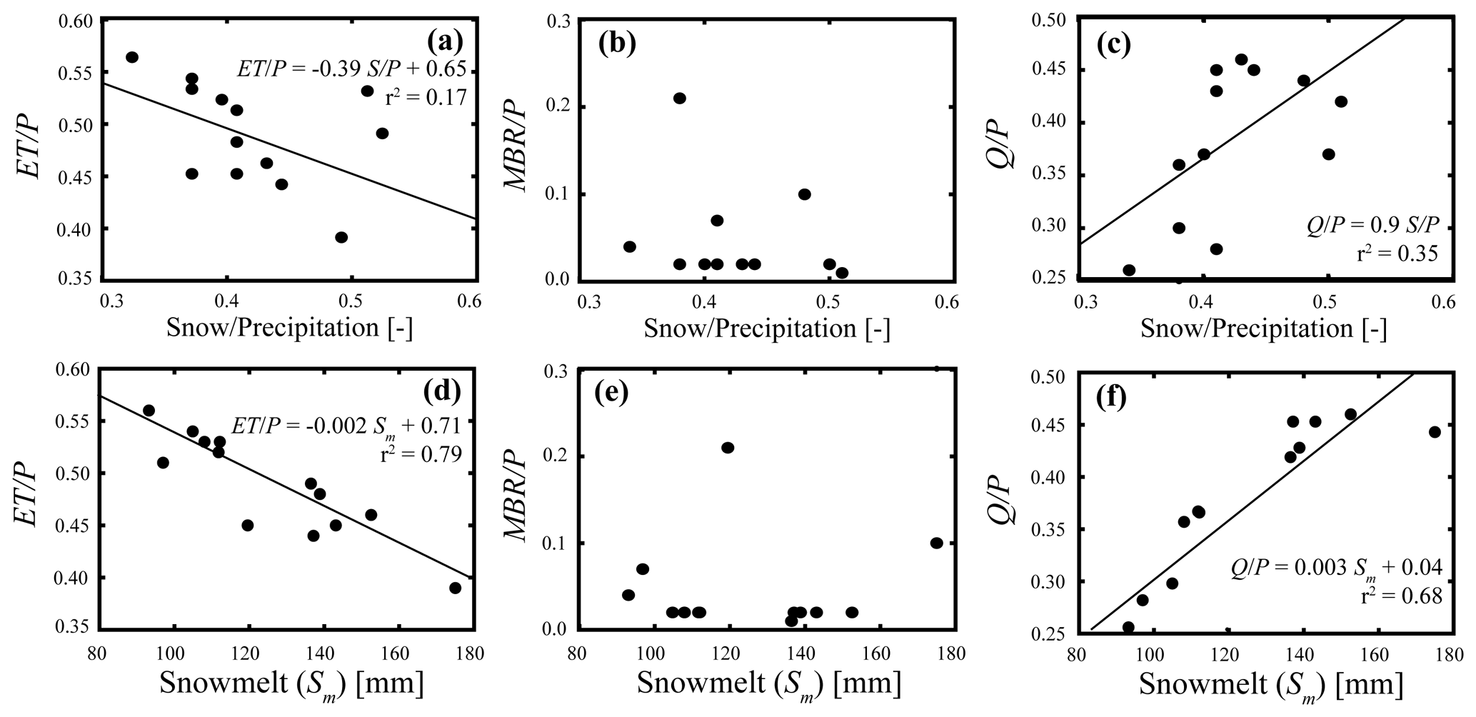
Figure 11 Scatterplots illustrating the relation between the annual snow $/$ precipitation ratio and ET $/$ P (a), MBR $/$ P (b), and $Q/P$ (c) ratios for WY2016. We also present the relation between the total annual snowmelt (S_m) and the ET $/$ P (d), MBR $/$ P (e), and $Q/P$ (f) ratios. Each point represents the value for the Kaweah Terminus watershed from each of the forcing scenarios in experiments 1–3. Black lines represent statistically significant (p<0.05) linear relationships.

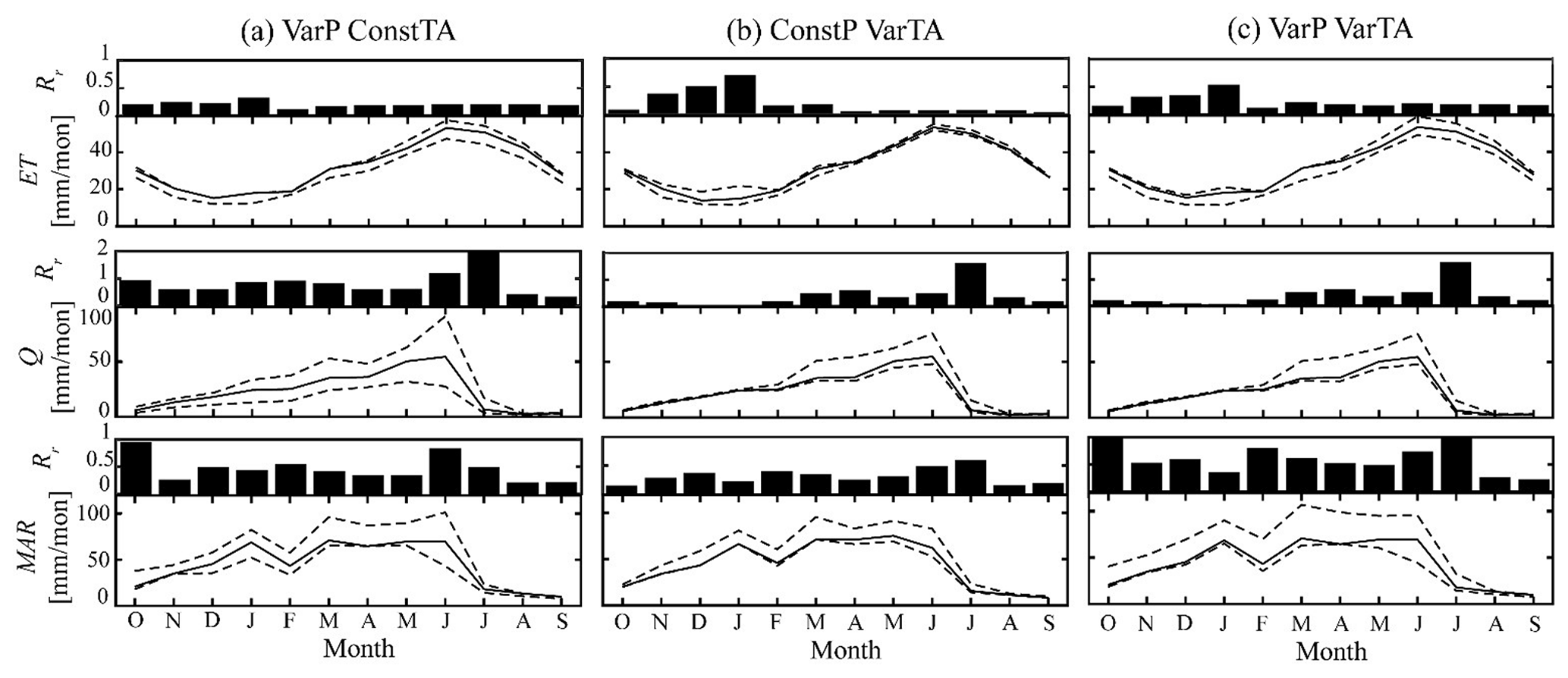
Figure 12 Monthly values of ET, Q, and MAR from the Kaweah Terminus watershed are presented for each of the three experiments (a) VarPConstTA, (b) ConstPVarTA, and (c) VarPVarTA for WY2016. The solid lines represent the values from the base case scenario, while the dashed lines present the range of values from the scenarios included in each experiment. Bars represent the relative range (R_r), defined as the range of simulated values for each experiment divided by the monthly value from the base case.

3.6 Interaction effects of combined changes to precipitation and air temperature on the water budget

Understanding the individual impacts of uncertainty in T_air and P forcings provides a foundation for how to manage uncertainty in meteorological forcings. However, as climate change is expected to alter both air temperature and precipitation, it is important to understand how uncertainty in both datasets combines to alter the simulated water budget. To test the extent to which the two sources of uncertainty superimpose, we compare the differences between hydrologic variables simulated with the base case scenario with simulations that alter both T_air and P (VarPVarTA, experiment 3). Initially, we use WY2016 simulations to calculate these sensitivities for the average value of each hydrologic variable over the Kaweah River watershed, while Q is represented at the Kaweah Terminus dam. Figure 14 presents the difference between the estimated and actual changes caused by the VarPVarTA simulations for each of the 3 simulation years. The difference can be interpreted as the strength of the interaction effects; i.e., a difference of 0.05 indicates that the interaction effects between T_air and P increased the value of the variable, v, by 5 %. Generally, the differences between estimated and simulated values are quite small, suggesting that the interaction effects between T_air and P uncertainty are small. Indeed, the majority of interaction effects are between −5 % and 5 %. The primary exception to this pattern is found in the variables related to groundwater, dS and R. The dS is the simulated variable with the largest variability in the interaction effects. For example, in WY2016 the Gridmet dataset results in interaction effects of −40 %, while the PRISM dataset results in interaction effects of 3 % in changes in subsurface storage. With the exception of the PRISM dataset, the interaction effects for dS are all negative (Fig. 14c). Additionally, across all four datasets the interaction effects decrease R, with an average value of −5.1 %. In both WY2011 and WY2014, the combination effects of precipitation and air temperature are largest for dS and R. This response in R, and subsequently dS, is expected as groundwater recharge is controlled by infiltration, ET, and soil moisture redistribution, and all of these processes are impacted by both P and T_air, creating a highly nonlinear response. This nonlinearity can be exacerbated by topography-driven flow that concentrates soil moisture and groundwater in convergent zones.

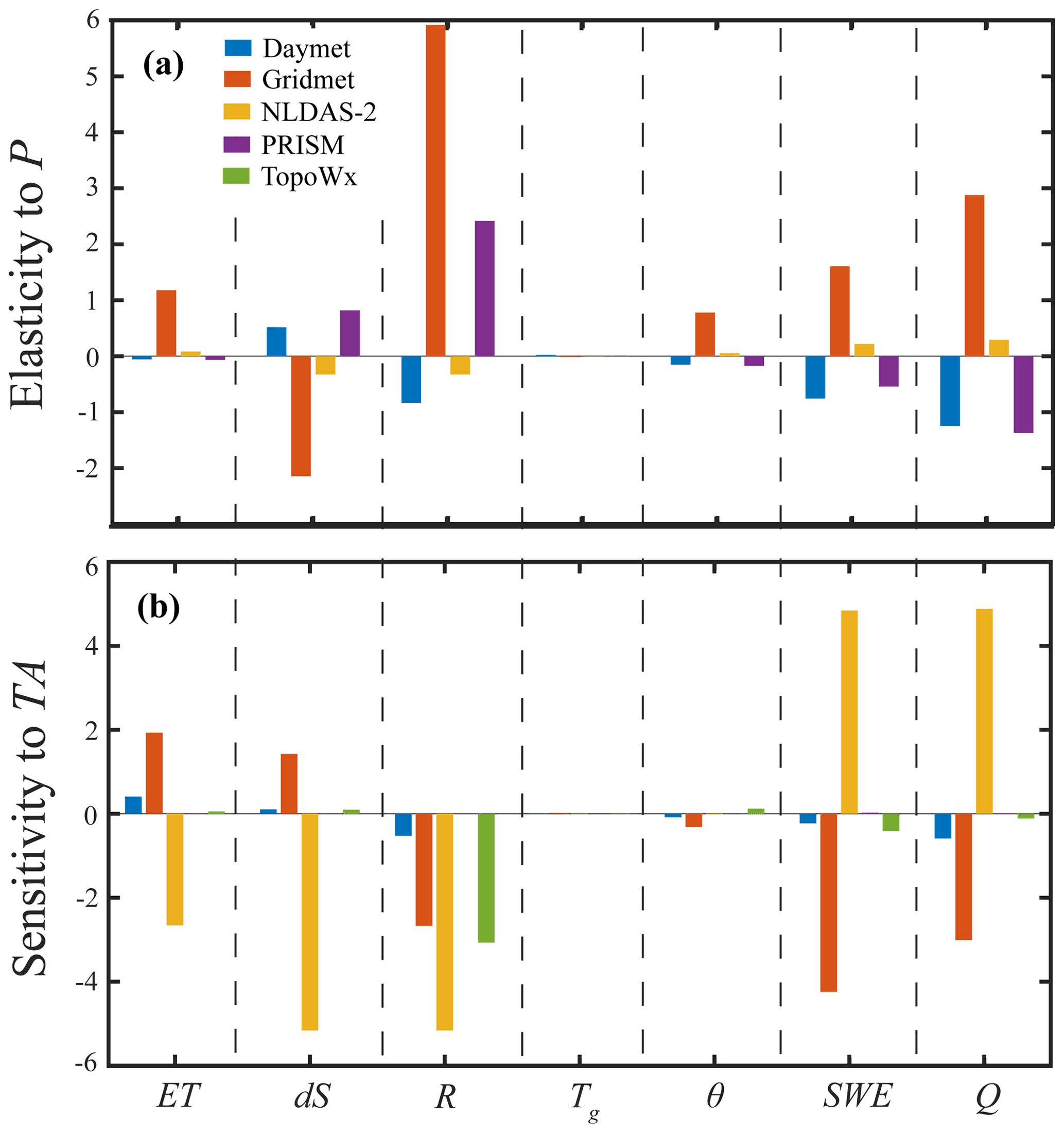
Figure 13 Elasticity (a) and sensitivity (a) of simulated hydrologic variables evapotranspiration (ET), change in subsurface storage (dS), potential recharge (R), land surface temperature (T_g), root zone soil moisture (θ), snow water equivalent (SWE), and streamflow (Q) to variability in precipitation and air temperature for WY2016. Each bar represents the average value from the Kaweah River watershed, except streamflow measured at the Kaweah Terminus dam. Elasticities were calculated using the scenarios from the VarPConstTA experiment, and sensitivities were calculated using the scenarios from the ConstPVarTA experiment.

3.7 Dependency of results on other uncertainty sources

In this study, we use a physically based, integrated hydrologic model, ParFlow.CLM, to quantify the impact of uncertainty in meteorological forcings on the simulated groundwater. However, the generality of results is influenced by multiple factors as described below. The results from this study are applicable to integrated surface water–groundwater models that implement the 3D Richards equation to simulate variably saturated subsurface flow across the entire subsurface and that have a fully integrated overland flow simulator. Previous studies have found that hydrologic sensitivities of land surface models can vary widely based on the model used (Vano et al., 2012). The land surface model we employ, the CLM, applies a threshold temperature of 2.5 ^∘C, below which precipitation falls as snow, which could have implications for our results. However, we expect its impact to be minimal, as most of the snow falls when the air temperature is much less than 2.5 ^∘C. Models with different rain–snow partitioning schemes, however, might find different sensitivities than what we describe here.

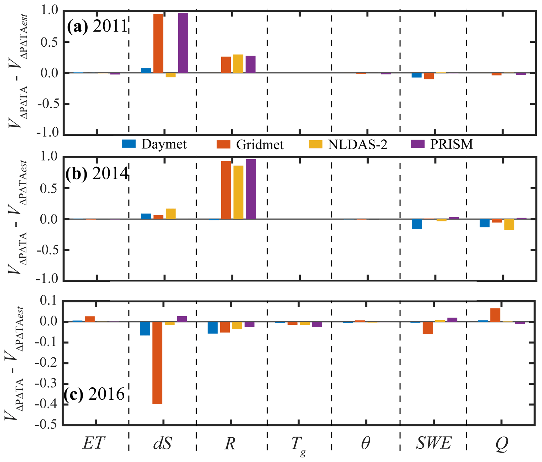
Figure 14 The difference between the predicted and actual changes from combined variability in P and T_air for WY2011 (a), WY2014 (b), and WY2016 (c).

Additionally, model parameterization is expected to affect the uncertainty in meteorological forcings. Previous results showed that three different conceptual models of the saprolite layer did not systematically impact the simulated groundwater response to precipitation variability (Schreiner-McGraw and Ajami, 2020). However, the simulated MFR depends on the subsurface permeability values assigned to the Central Valley aquifer in the piedmont slope region. Our hydraulic parameter values are based on drill core data and a previously calibrated hydrologic model (Faunt, 2009), but hydraulic conductivity values may be too high, causing overestimation of simulated MFR (Brush et al., 2013). Historical observations under pre-development conditions suggest that the Kaweah River branched into several smaller distributaries, some of which did not flow all the way to the historic Tulare Lake (Anon, 2007; Hall, 1886). These observations suggest that our MFR estimates from the Kaweah River are reasonable but are likely overestimated due to coarse horizontal model resolution resulting in streambeds that are unreasonably wide and potentially overestimated hydraulic conductivity of the Central Valley sediments. Conversely, the coarse resolution of the model may result in an underestimation of MFR via small channels and first-order watersheds located on the piedmont slope (Schreiner-McGraw and Vivoni, 2018).

In addition to the hydrologic model structure, the selection of the study domain will affect our results, and we would expect different sensitivities depending on the topography and vegetation type in other regions. Despite the site-specific nature of our study, the evergreen forest in our study watershed is broadly representative of evergreen forests in the mountainous, western United States. In our simulations, the weathered bedrock zone is the most hydrologically active region of the subsurface, which has been observed as a feature of the Sierra Nevada (Holbrook et al., 2014). This is a common pattern in other mountainous regions with low-permeability bedrock (Pfister et al., 2017; Jencso et al., 2009; Spencer et al., 2019). Previous work in mountainous regions with low-permeability bedrock has found that storage can respond quickly to meteorological conditions as a result of the low permeability and low storage capacity (Pfister et al., 2017) and would impact the overall hydrologic response. Further research to examine how meteorological forcing uncertainty propagates into groundwater systems across a range of bedrock conditions is warranted.

4 Summary

In this paper, we examine the propagation of uncertainty in the meteorological forcings, precipitation, and air temperature into groundwater recharge simulated with the integrated hydrologic model, ParFlow.CLM. We use the Kaweah River watershed as a study domain to (1) quantify groundwater recharge from the mountain system and assess which recharge pathway is most sensitive to meteorological variability under a range of hydroclimatic conditions (wet, dry, and average), (2) determine whether uncertainty contained in common P or T_air gridded datasets has a larger impact on the simulated water budget, and (3) evaluate the strength of interaction effects when both P and T_air are uncertain. In the course of this analysis, we perform three sets of model experiments by altering forcing datasets to compare them with our base case scenario forced with the mean P and mean T_air for three distinct hydroclimatic conditions. These experiments include variable P constant T_air (VarPConstTA), constant P variable T_air (ConstPVarTA), and variable P variable T_air (VarPVarTA).

Given that the P datasets differ in their total annual precipitation by up to 30 % and that variability in the spatial distribution of precipitation is large, one might expect that the choice of P dataset would be more important than the choice of T_air dataset. Our analysis revealed that in a mountainous system, the impact of uncertainty in gridded P datasets is similar to the impact of uncertainty in available T_air datasets. The range of values in the simulated water budget partitioning for the VarPConstTA scenarios and the ConstPVarTA scenarios is comparable. This result is attributed to the impact of air temperature on snow processes. Variability in T_air creates variability in the partitioning of precipitation into rain and snow. This partitioning alone impacts the water budget, where higher ratios of snow $/$ rain result in more potential recharge. Additionally, air temperature impacts the snowmelt rate, and the total amount of snowmelt is a strong control of the water budget partitioning, with higher snowmelt leading to less ET and more potential recharge, which is discharged from the mountain system into streamflow. We calculate the sensitivity and elasticity of changes in the water budget to changes in T_air and P, respectively. We find that groundwater recharge and storage changes are highly sensitive to both changes in T_air and P. Our results demonstrate that the high levels of uncertainty in both T_air and P gridded datasets have profound impacts on the water budget simulated by an integrated hydrologic model where surface and subsurface processes are coupled.

The uncertainty in the simulated water budget caused by the separate uncertainty in the T_air and P forcing datasets is largely superimposed when the model is forced with variable T_air and variable P. For most water budget components, the interaction effects of T_air and P uncertainty reduce the combined impact of uncertainty by less than 5 %; i.e., the variability in the simulated water budget caused by combined changes to T_air and P forcing is within 5 % of the sum of the variability from individual changes. The exception to this result is found in the groundwater system. Potential groundwater recharge and changes in subsurface storage exhibit larger interaction effects than the surface water budget. This is attributed to the role of topography in controlling lateral subsurface flow in the shallow groundwater system. The uncertainty in groundwater recharge rates is highest in regions of convergent topography for all three experiments. However, the uncertainty in these regions is much higher when variable T_air forcings are used. This is because the topography concentrates water in these locations, so that ET becomes energy limited. As a result, variability in T_air creates more variable ET and recharge.

Finally, all of the recharge pathways present in the mountainous Kaweah watershed, MAR, MBR, and MFR, are more sensitive to changes in P than changes in T_air, and these results are consistent across the three meteorological conditions. It should be noted, however, that comparisons are difficult due to different units for P and T_air sensitivities. The higher sensitivity to the P dataset is because these pathways largely depend on snowmelt, and precipitation is concentrated in the winter in high-elevation regions where the air temperature remains well below freezing during this time period. The MAR pathway is less sensitive to changes in P than the other pathways, particularly when MAR is derived from rainfall. Our simulations suggest that mountain system recharge to the Central Valley aquifer is a significant portion of the water budget regardless of the meteorological forcing dataset used. Indeed, during an approximately average precipitation year, MFR contributes between 186 and 504 mm yr⁻¹ of recharge from the Kaweah Terminus watershed to the Central Valley aquifer, and a large fraction of the Kaweah Terminus watershed water budget (9 %–72 %, depending on the year and forcing datasets used) becomes MFR. In our simulations, MFR is the primary pathway via which the mountain system recharges the Central Valley aquifer, accounting for 85 %–99 % of the total recharge. The high uncertainty in subsurface geologic structure and parameters, however, creates large uncertainties in the quantities of MBR. Overall, the results from this study highlight the importance of uncertainty in forcing datasets when simulating the groundwater response to climate change. The magnitude of simulated changes in the groundwater recharge due to meteorological forcing uncertainty highlights the need for hydrologists to improve gridded datasets to improve our understanding of how meteorological variability propagates into groundwater in topographically complex mountain systems.

Appendix A

Figure A1 displays the estimated changes to the simulated hydrologic variables ($v_{\mathrm{\Delta }P\mathrm{\Delta }{T}_{{\text{air}}_{\text{est}}}})$, relative to the base case scenario, if the impact of uncertainty from the ConstPVarTA and VarPConstTA scenarios were additive. Figure A1 displays the estimated (a) and actual (b) changes caused by the VarPVarTA simulations, and Fig. A1c presents the difference between the estimated and actual changes. The difference can be interpreted as the strength of the interaction effects; i.e., a difference of 0.05 indicates that the interaction effects between T_air and P increased the value of the variable, v, by 5 %.

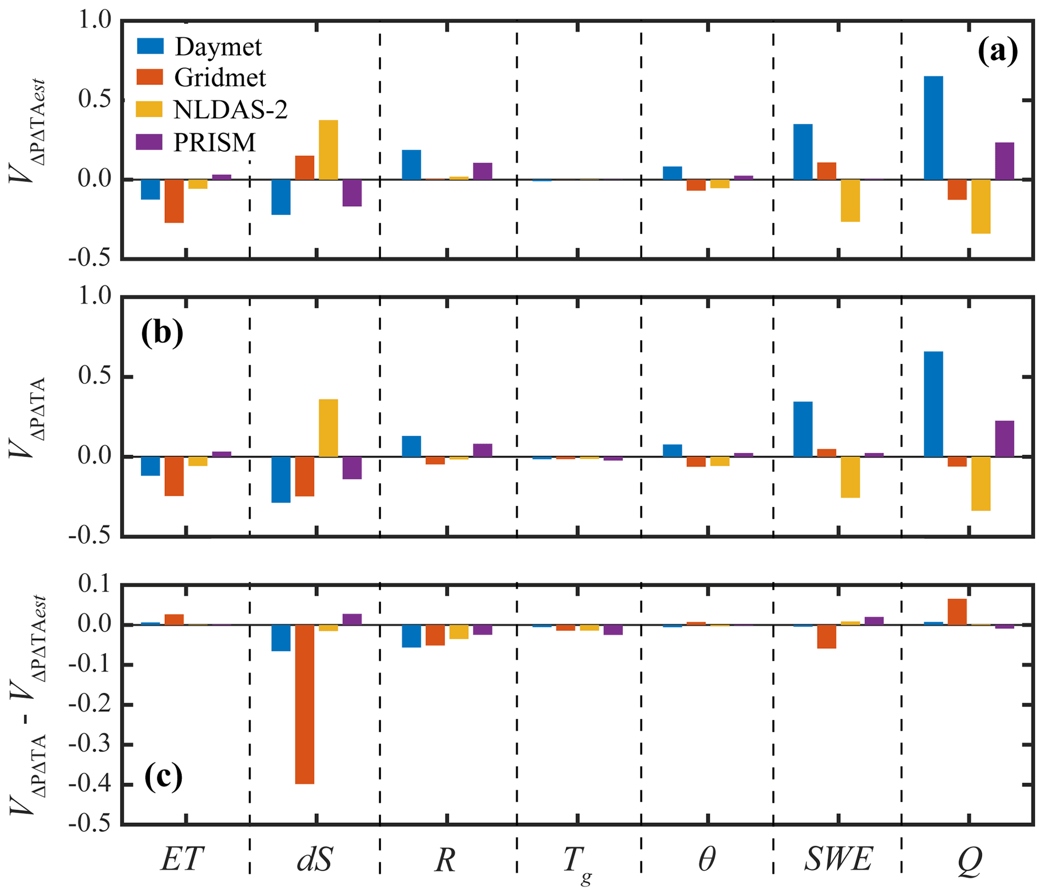
Figure A1 Demonstration of the method to calculate the interaction effects between P and T_air uncertainty using WY2016. (a) The estimated relative difference in the hydrologic variables evapotranspiration (ET), change in subsurface storage (dS), potential recharge (R), land surface temperature (T_g), root zone soil moisture (θ), snow water equivalent (SWE), and streamflow (Q) if the effects of air temperature and precipitation changes are linearly additive. (b) The relative difference between the base case and each of the VarPVarTA scenarios. (c) The difference between the predicted and actual changes from combined variability in P and T_air.