the Creative Commons Attribution 4.0 License.
the Creative Commons Attribution 4.0 License.
 | 28 Feb 2022
Temporally resolved coastal hypoxia forecasting and uncertainty assessment via Bayesian mechanistic modeling
Alexey Katin
Dario Del Giudice
Daniel R. Obenour
Low bottom water dissolved oxygen conditions (hypoxia) occur almost every summer in the northern Gulf of Mexico due to a combination of nutrient loadings and water column stratification. Several statistical and mechanistic models have been used to forecast the midsummer hypoxic area, based on spring nitrogen loading from major rivers. However, sub-seasonal forecasts are needed to fully characterize the dynamics of hypoxia over the summer season, which is important for informing fisheries and ecosystem management. Here, we present an approach to forecasting hypoxic conditions at a daily resolution through Bayesian mechanistic modeling that allows for rigorous uncertainty quantification. Within this framework, we develop and test different representations and projections of hydrometeorological model inputs. We find that May precipitation over the Mississippi River basin is a key predictor of summer discharge and loading that substantially improves forecast performance. Accounting for spring wind conditions also improves forecast performance, though to a lesser extent. The proposed approach generates forecasts for two different sections of the Louisiana–Texas shelf (east and west), and it explains about 50 % of the variability in the total hypoxic area when tested against historical observations (1985–2016). Results also show how forecast uncertainties build over the summer season, with longer lead times from the nominal forecast release date of 1 June, due to increasing stochasticity in riverine and meteorological inputs. Consequently, the portion of overall forecast variance associated with uncertainties in data inputs increases from 26 % to 41 % from June–July to August–September, respectively. Overall, the study demonstrates a unique approach to assessing and reducing uncertainties in temporally resolved hypoxia forecasting.
- Article
(1216 KB) - Full-text XML
-
Supplement
(12011 KB) - BibTeX
- EndNote


The northern Gulf of Mexico has one of the largest hypoxic zones in the world, forming virtually every summer over the last 3 decades (Rabalais and Turner, 2019). Hypoxic, or dead, zones occur when dissolved oxygen concentrations fall below critical thresholds (e.g., 2 mg L−1), threatening aquatic ecosystems (Craig, 2012; Craig and Crowder, 2005; Thronson and Quigg, 2008), fisheries (Purcell et al., 2017; Smith et al., 2017), and coastal economies (Díaz and Rosenberg, 2011). The two major causes of hypoxia in the Gulf are water column stratification and nutrient loadings (Krug, 2007; Obenour et al., 2012; Rabalais et al., 2002), which are both influenced by Mississippi and Atchafalaya river discharges. Additionally, wind controls both the structure of the river plume (Hetland, 2005) and the rates of oxygen supply to the water column (Fennel et al., 2013; Justić et al., 1996). Overall, a complex combination of biophysical factors, including long-term accumulation of organic matter (Del Giudice et al., 2020; Turner et al., 2008) and short-term events like storms and droughts (Bianchi et al., 2010), control hypoxia dynamics in the northern Gulf.
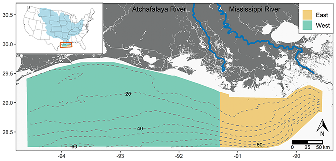
Figure 1Map of the study area located in the northern Gulf of Mexico. The Mississippi and Atchafalaya river basin (top left; light blue filled) is used to estimate monthly precipitation and temperature. Dashed gray lines indicate isobaths (meters).
Mathematical models are useful for elucidating important relationships between hypoxia and environmental drivers and for evaluating the consequences of possible actions to improve water quality (Justić and Rose, 2017). The approaches developed to predict hypoxia in the Gulf of Mexico included statistical regressions (Forrest et al., 2011; Greene et al., 2009; Turner et al., 2012) and both parsimonious (Obenour et al., 2015; Scavia et al., 2013) and complex (Justić and Wang, 2014; Yu et al., 2015) mechanistic models. Among these alternatives, parsimonious process-based models attempt to balance biophysical detail with computational efficiency and resilience to overfitting. When embedded in a Bayesian framework, these models describe eutrophication processes and hypoxia formation while enabling data-driven parameter estimation and rigorous uncertainty analysis (Ménesguen and Lacroix, 2018). The latter is especially important for assessing our confidence in the potential outcomes of environmental change and management decisions (Reichert and Borsuk, 2005; Schuwirth et al., 2019).
Currently, a probabilistic ensemble of four models is used to inform stakeholders and fishery managers about the expected extent of the northern Gulf hypoxic zone (Scavia et al., 2017). This ensemble provides predictions with estimates of uncertainty of the midsummer hypoxic area (HA). However, the forecast lacks dynamic oxygen predictions over the summer season. The lack of subseasonal information on dissolved oxygen variability has been identified as an important limitation in understanding how hypoxia affects fisheries in the region, which occurs primarily during the summer season but are highly dynamic in space and time (Langseth et al., 2016; Purcell et al., 2017; Smith et al., 2014). Laurent and Fennel (2019) used a weighted aggregation of seasonal hindcasts generated by a three-dimensional model to produce spatially and temporally resolved seasonal hypoxia forecasts but without accounting for uncertainties related to the model parameterization (Mattern et al., 2013). Furthermore, the aforementioned forecasting approaches are informed only by observed spring nutrient loading, without considering variability in spring wind conditions (Obenour et al., 2015) or projected summer river discharge and loading.
Here, we use an existing mechanistic model, calibrated within a Bayesian inference framework, to forecast the temporal dynamics of hypoxia in the northern Gulf over the summer season. The model was initially developed by Obenour et al. (2015) and later enhanced by Del Giudice et al. (2020; hereafter referred to as DMO20). While the model performed well in hindcasting, its ability to forecast hypoxia forward in time has not been explored. In order to provide sufficient lead time for environmental planning and fisheries management, we produce a June–September hypoxia forecast based on data available at the end of May. The main objectives of this study are to (a) develop daily forecasted spatial mean bottom water dissolved oxygen (BWDO) concentrations and HA estimates for targeted portions of the Louisiana–Texas shelf with accompanying measures of uncertainty, (b) understand the major sources of forecast uncertainty, (c) characterize how forecast accuracy degrades over time, and (d) explore how different applications of spring–summer riverine and meteorological data influence forecast performance.
We first outline the underlying model and required data inputs. Next, we describe the proposed forecasting procedure, along with regression models, to project discharge and nitrogen loading over the summer. Third, we describe the approach to evaluating the BWDO and HA forecast performance and analyze how the forecast varies in relation to alternative combinations of data inputs.
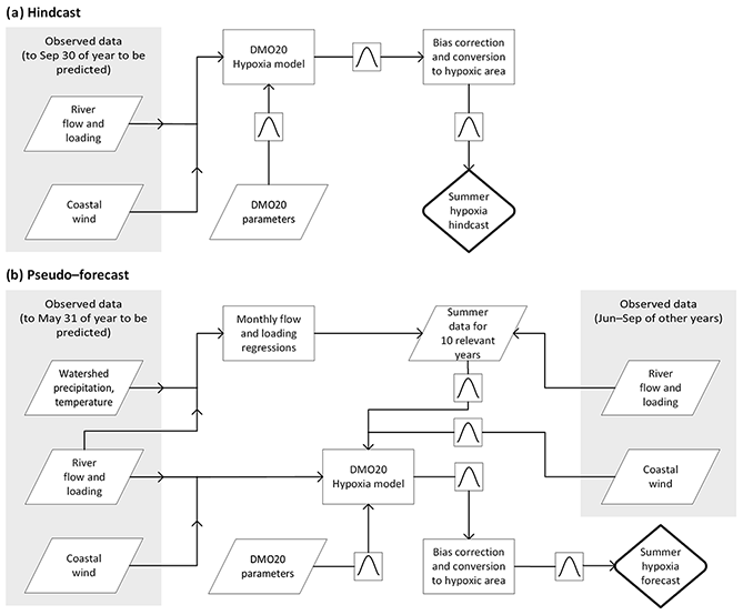
Figure 2Flowchart summarizing processes and inputs required to generate the hypoxia hindcast (a) and pseudo-forecast (b) for a given year. Parallelograms represent data inputs and Bayesian posterior parameter distributions. Rectangles represent forecasting computations, and squares with bell-shaped curves indicate steps that propagate uncertainty (including stochastic hydrometeorology).
2.1 Bayesian mechanistic model and bias adjustment
The hypoxia forecast is based on the model described in DMO20, which has a parsimonious, mechanistic formulation and coarse spatial resolution. Specifically, the model represents the Louisiana–Texas shelf from Galveston Bay to the Mississippi River delta, which has been divided into four compartments. The western and eastern sections are separated at the Atchafalaya River mouth (Fig. 1), while the water column of each section is divided by the pycnocline into two layers, assuming that the discharge and nutrient loadings are transported within the top layer. Additionally, the wind speed and direction control the distribution of flow and loadings between the eastern and western sections and the rate of reoxygenation across the pycnocline. The biogeochemistry is based on the transformation of bioavailable nitrogen (sum of nitrate, nitrite, ammonia, and 12 % organic nitrogen; Obenour et al., 2015) into organic matter, which settles to the bottom layer and is subject to aerobic decomposition. BWDO is depleted due to both near- and long-term oxygen demands, reflecting the effects of nitrogen loadings over different timescales. Therefore, the model uses both recent inputs of daily discharge, loading, and wind (up to 90 d before the date of prediction) and long-term November–March loading. In addition, the Bayesian calibration framework provides systematic estimation of model parameters and their uncertainties (Table S1 in the Supplement). All major equations of DMO20, including regressions to convert BWDO to HA, are presented in Sect. S1 in the Supplement. Estimates of BWDO and HA generated by DMO20, using known nutrient and hydrometeorological inputs throughout the summer, are hereinafter referred to as hindcasts (Fig. 2a).
Prior to developing the daily forecast, we examined DMO20 hindcasts for systematic biases during specific months and found that estimated BWDO was (0 %–20 %) lower than observations for the western section of the shelf in June. However, this discrepancy diminished towards the end of the month (Sect. S2). This apparent bias, which could be due to an overestimation of June oxygen demands or other structural limitations within DMO20, was corrected using a linear regression, with the day number (June 1 to June 30) as a predictor and the BWDO adjustment as the response (Fig. S2.1). This adjustment factor was applied to all June model predictions (hindcasts and forecasts), unless otherwise indicated.
2.2 Data
The forecast utilized the same observational data inputs described in DMO20, including monthly discharge and nitrogen loading from the U.S. Geological Survey (USGS, 2019), daily discharge from the U.S. Army Corps of Engineers at Simmesport and Tarbert Landing (USACE, 2019), and wind velocities from the National Data Buoy Center (NDBC, 2019). Additionally, monthly precipitation and temperature were obtained from gridded data for the Mississippi River basin (Hart and Bell, 2015; Schwartz, 2012). For both shelf sections, estimates of mean BWDO and HA with associated uncertainties were obtained using the space–time geostatistical model of Matli et al. (2018). This model relies on BWDO samples from ship-based monitoring cruises, and similar to DMO20, we only used the geostatistical estimates corresponding to times of these cruises (when uncertainty is typically lowest). At least one monitoring cruise was conducted for every year of the study period (1985–2016), and there were a total of 149 cruises (34 in June, 63 in July, 35 in August, and 17 in September).
2.3 Forecast procedure
To capture the uncertainty in hydrometeorology, nutrient loading, model parameters, and residual error, the forecast for a given year was determined through 1000 Monte Carlo simulations (Fig. 2b) implemented in R (R Core Team, 2019). Each simulation included a random draw from the Bayesian joint posterior parameter and error distribution of the mechanistic model (DMO20) and the uncertainty in the regressions for bias correction and for converting BWDO to HA. The simulations used actual November–May riverine and meteorological inputs for the forecast year, since these inputs would be known by the nominal forecast release date of 1 June. However, summer (June–September) inputs were sampled from historical records of multiple years (always omitting the forecast year). To retain the temporal correlation in these inputs, data were sampled in blocks (i.e., the complete daily time series for each summer). As wind conditions cannot be accurately forecasted beyond 10 d (Zhang et al., 2019), summer wind velocity data were sampled from the complete historical record (1985–2016).
Summer riverine inputs can potentially be projected in advance through regression (Sect. 2.4). Thus, riverine time series were sampled from only the 10 most relevant historical years. For each historical year, relevancy to the forecast year was determined by computing the differences between the summer historical records and the regression-projected discharge and bioavailable nitrogen loading (Sect. 2.4). Monthly projections and observations were standardized, based on the mean and standard deviation of the historical data for each summer month, so that the differences in loading and flow could be combined on the same unitless scale. The 10 years with the smallest aggregated differences were selected as the relevant years for use in the Monte Carlo simulations.
2.4 Regressions for June–September discharge and loading
Regression modeling was used to project riverine inputs, which were employed to constrain the historical records used in the Monte Carlo simulations to relevant years (Sect. 2.3; Fig. 2b). June, July, August, and September river discharge (QA for Atchafalaya and QM for Mississippi, m3 s−1) and bioavailable nitrogen loading (LA and LM, T mo−1) were estimated through multiple linear regression. The candidate predictor variables (predictors) included the monthly (January–May) and 4-month average (January–April) discharge, loading, total river basin precipitation (P; cm), and river basin temperature (T; ∘C). Response variables were square root transformed to account for the skewness of their distributions and comply with the error normality assumption for linear regression (Faraway, 2015). Predictors for each model were selected using the Bayesian information criterion (BIC) through an exhaustive search (Lumley, 2017). BIC prioritizes models based on log likelihood while penalizing for the number of parameters to prevent overfitting (Faraway, 2015). The performance of the regression was measured by the coefficient of determination, R2, in the square-root-transformed space. If any of the 16 regressions had R2 < 30 %, then the associated month and variable was excluded from determining relevant years for hypoxia forecasting (Sect. 2.3). To further check the validity of these regressions, we performed leave-one-out cross-validation (LOOCV), where we excluded the years one by one, calibrated the models to the reduced dataset, and predicted the values for the excluded year. Cross-validation is commonly used to evaluate the ability of models to predict out of sample and to prevent overfitting (Berrar, 2019).
2.5 Forecast assessment
The forecasting approach was applied to the complete historical record (1985–2016, excluding the summer input data of the forecast year from the Monte Carlo simulation). This retrospective forecast (i.e., pseudo-forecast) performance was evaluated through comparison of the daily forecasted values with both hindcasted (generated by DMO20) and geostatistically estimated (referred to as observed, for brevity) BWDO and HA for the two shelf sections. The approach also allowed for the determination of the 95 % interquartile ranges (IQR) of the pseudo-forecasts, accounting for uncertainties in parameters, model residuals, BWDO to HA transformation, and bias adjustment, as well as the stochasticity in riverine and meteorological inputs (Sect. 2.3).
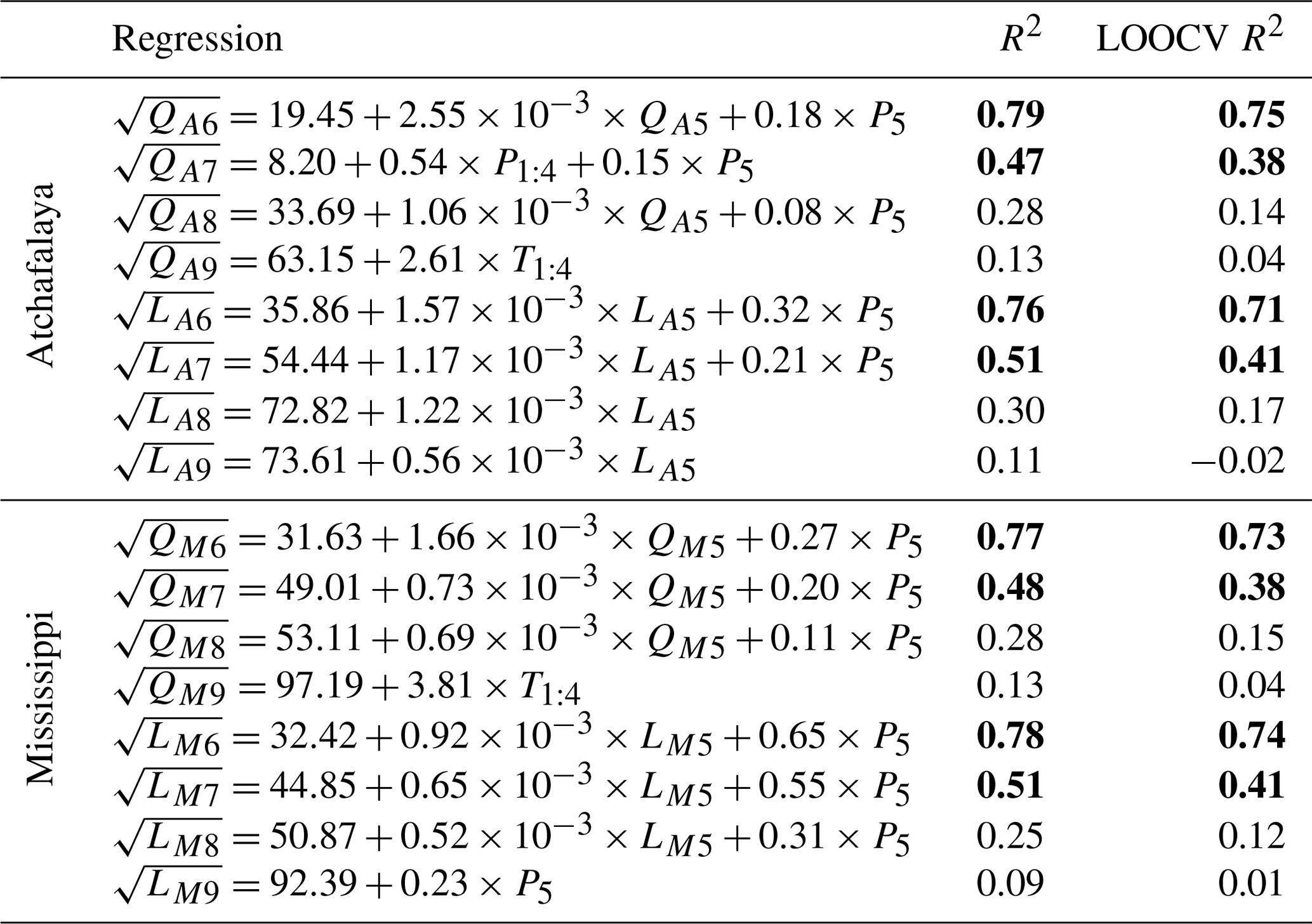
Table 1Regressions for monthly Atchafalaya and Mississippi river discharge (QA and QM, m3 s−1) and bioavailable nitrogen loading (LA and LM; Mg mo−1). Variable subscript numbers represent months. For example, P1:4 represents average Mississippi River basin precipitation for January–April. R2 values are presented for the model calibrated to all data and for the leave-one-out cross-validation (LOOCV). Bold R2 values (> 0.30) indicate models used for selection of relevant years in hypoxia forecasting.
We also assessed how the inclusion of various hydrometeorological inputs affected the pseudo-forecast accuracy and uncertainty. Specifically, we compared four cases with different types of spring–summer wind and summer riverine data. Case 1 included summer riverine and spring–summer wind records randomly sampled from the complete historical data (thus, they are treated as unknown, consistent with conventional Gulf forecasting approaches). Case 2 was similar to Case 1, except that it included actual spring wind data (to 31 May). Case 3 was also similar to Case 1, except that it used summer riverine records sampled from only the 10 most relevant historical years, as determined from the regression projections (Sect. 2.4). Finally, Case 4 (our proposed approach; Fig. 2b) used both actual spring wind data and riverine records from the 10 most relevant years.
3.1 Monthly discharge and loading projections
Multiple linear regressions predict average monthly (June to September) summer river discharge and bioavailable nitrogen loading at each river outlet. The performance of these 16 regressions generally decreases from the beginning to the end of summer (Table 1), reflecting the increasing temporal gap (i.e., lead time) between the available spring predictors and the forecast response. For instance, the regressions explain 78 % and 9 % of the variability in (square root transformed) Mississippi River bioavailable nitrogen loading in June and September, respectively. The residuals for all selected models appear evenly distributed, with minimal heteroscedasticity (Fig. S3.1–S3.4) and mostly weak serial correlation of residuals (Pearson lag 1 correlations ranging from –0.02 to 0.35). The predictive variables chosen via exhaustive BIC selection include May discharge (QA5 or QM5) or bioavailable nitrogen loading (LA5 or LM5) in 13 of the 16 models. In other words, high flow and nutrient loading in May is indicative of high flow and nutrient loading in summer. However, the most consistent individual predictor (present in 12 out of 16 regressions) is the Mississippi River basin precipitation in May (P5), likely due to the hydrologic lag between rainfall and basin discharge. Note that the correlation between P5 and May discharge is relatively weak (r = 0.36 for both rivers), while the correlations between P5 with June and July discharge are r = 0.77 and r = 0.66, respectively, suggesting an average basin response time of 1–2 months. This lag is generally consistent with a previous study that identified a strong positive correlation between March–May precipitation and May–June nitrogen flux in the basin (Donner and Scavia, 2007). Additionally, the strong influence of lagged watershed precipitation on nitrogen loading has been confirmed for other river basins (Gentry et al., 2014; Hinsby et al., 2012; Sinha and Michalak, 2016). At the same time, the regressions for August and September flow and loading perform particularly poorly in the LOOCV (R2 < 0.2), indicating they are less robust and have little predictive capacity relative to the models for earlier months (Table 1). Therefore, only the eight regressions for June and July discharge and bioavailable nitrogen loading are used for screening and constraining riverine inputs for subsequent hypoxia forecasting.
3.2 Forecast skill
After constraining historical riverine inputs (to the 10 most relevant years, excluding the forecast year), based on the discharge and loading regressions for each forecast year, the hypoxia model (DMO20) is run to obtain daily hypoxia predictions (Fig. 3; top). Over the 32-year record, these pseudo-forecasts explain 66 % and 64 % of the variability in hindcasted BWDO (i.e., DMO20 model predictions assuming all inputs are known throughout the summer) for the western and eastern sections, respectively. After the transformation of BWDO to HA, the pseudo-forecast explains 68 % of variability in hindcasted HA for each section (Fig. S4.1). Overall, the pseudo-forecast explains 71 % and 77 % of the variability in hindcasted total shelf-wide HA and mean BWDO, respectively.
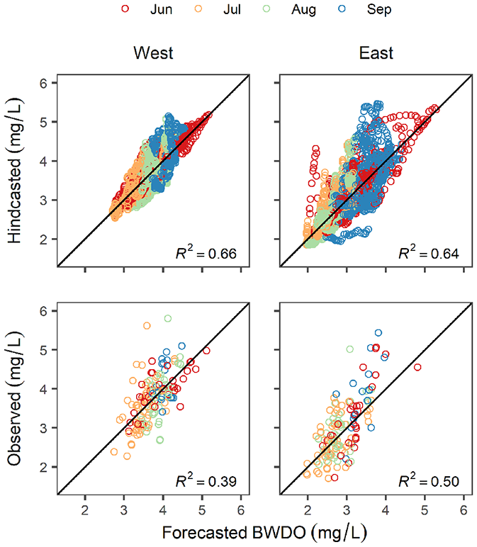
Figure 3Daily hindcasted BWDO (predicted for every summer day from DMO20, 1985–2016, assuming that the hydrometeorology and loading is known throughout the summer) and observed BWDO (geostatistically estimated from monitoring cruises) versus forecasted BWDO for western and eastern shelf sections. The diagonal line represents the perfect prediction.
Pseudo-forecasts can also be compared to observed (geostatistically estimated) BWDO and HA at the times of monitoring cruises (Fig. 3; bottom). The forecasted BWDO fits moderately well to the observations with an R2 of 0.39 and 0.50 for the western and eastern sections, respectively. When BWDO is transformed to HA, the pseudo-forecast explains 41 % and 48 % of variability in observed HA in the western and eastern sections, respectively (Fig. S4.1), which is similar to the hindcast explanatory power of 46 % and 58 % (as in DMO20). In comparison, hindcasting studies using three-dimensional models have generally explained a lower (27 %–37 %) percentage of the variability in the Gulf BWDO but at finer spatial resolution (Fennel et al., 2016). To our knowledge, this is the first time that Gulf hypoxia forecasts have been rigorously compared to observations across the entire summer season (June–September). Previous studies have generally focused on assessing forecast performance relative to the Louisiana Universities Marine Consortium midsummer shelf-wide hypoxia cruises, which typically take place within a 2-week window beginning in late July (Laurent and Fennel, 2019; Scavia et al., 2017).
A tighter selection of relevant years for forecast generation may produce more accurate forecasting results but may capture less of the true stochasticity in the hydrometeorology. If the forecasting approach is revised to include only the 5 most relevant years, the predictive accuracy slightly improves, based on comparisons with hindcasted values of total shelf-wide HA (the variance explained increases from 71 % to 73 %), while there is virtually no improvement based on comparisons with observed HA. At the same time, the uncertainty (standard error) for the population variance increases by a factor of 1.5 when using 5 years instead of 10 years (Benhamou, 2018). Therefore, using 10 relevant years appears to provide a more reasonable balance between predictive accuracy and uncertainty characterization, though this could be explored further in future research.
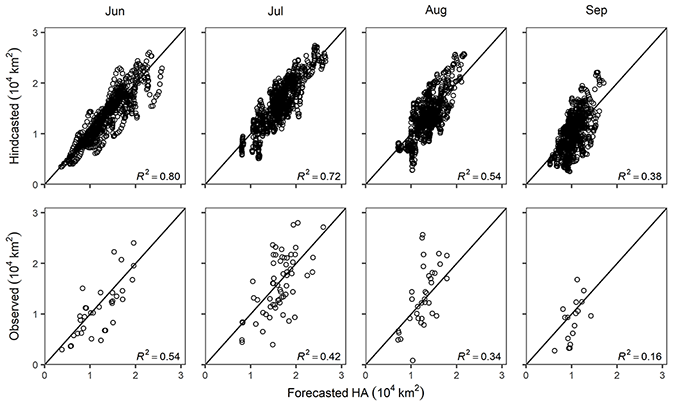
Figure 4Month-by-month comparison of the daily hindcasted (top) and observed (geostatistically estimated; bottom) shelf-wide HA versus pseudo-forecasted HA. The diagonal line represents perfect prediction.
Forecasting performance gradually degrades with longer lead times. The ability of pseudo-forecasts to match DMO20 hindcasts of shelf-wide HA declines by about 50 % (comparing R2 values; Fig. 4; top) from June to September due to increasing uncertainty in riverine and meteorological inputs toward the end of the summer season. In comparison, the ability of forecasts to match actual observations declines by nearly 70 % (Fig. 4; bottom). Forecasts and hindcasts benefit from the same seasonal patterns inherent to the DMO20 model structure, while observations may deviate from these patterns due to additional drivers of variability not captured in the mechanistic formulation. Moreover, the geostatistical observations have their own uncertainties, depending on the coverage of each monitoring cruise (Matli et al., 2018).

Figure 5Daily pseudo-forecasts of HA for the western and eastern sections in 1993 (a, b) and 2009 (c, d), including the 95 % IQR of the predictive distribution, distinguishing between (i) parameter, (ii) riverine and meteorological inputs, (iii) mechanistic model residual error, and (iv) regressions related to transformation of BWDO to HA and bias adjustment uncertainties (shades of gray from lightest to darkest). The yellow dashed line is the hindcasted estimate, the black dashed line is the 32 year average hindcast, and the orange points and error bars represent the mean and associated 95 % confidence interval of the (geostatistically estimated) hypoxia observations.
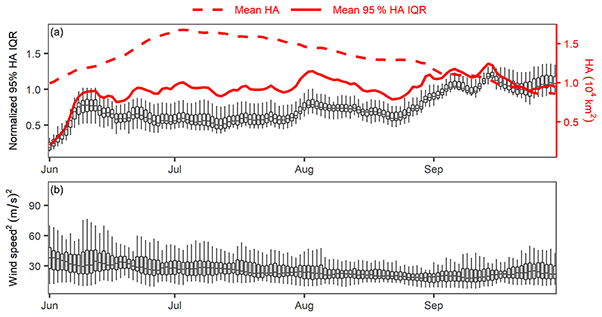
Figure 6(a) Box plots represent the daily pseudo-forecasted normalized IQR (IQR/HA), including the uncertainty due to variability in the parameters, riverine inputs, and meteorology. The red dashed and solid lines show the daily mean HA and (non-normalized) IQR, respectively. (b) Box plots show 14 d weighted-average-squared wind speed near the western shelf section. Box plots represent the interannual variability in the results. The center of each box is the median, while the whiskers extend to the extreme value or 1.5 times the IQR of the corresponding variable (whichever is less).
Our forecast quantifies predictive uncertainty associated with the Bayesian parameter estimates and residual errors, summer model inputs, bias adjustment, and transformation of BWDO to HA (Figs. 5 and S5.1–S5.11). The results indicate that the 95 % IQR for the western section is, on average, 2.6 times higher than for the eastern section, due to the greater overall size of the western section (and greater HA) and the complex effect of both river outfalls (Atchafalaya and Mississippi) on BWDO in this section (DMO20). Although the forecasts generally follow the shape of the hindcasts over time, some dissimilarities exist due to the hydrometeorological variability (Fig. 5). The pseudo-forecast captures the large HA during summer 1993 that was caused by extremely high May–September river flow and nutrient loadings (Larson, 1997). Interestingly, however, the pseudo-forecast in 2009 overpredicts HA in the western section (two observations are outside of the 95 % IQR), due to unusually strong westerly summer winds in this year (Turner et al., 2012). Generally, high wind stress increases water column reaeration and disrupts stratification (Justić and Wang, 2014; Obenour et al., 2015), while upwelling westerly winds disperse the river plume offshore, reducing the consequent oxygen demand (Feng et al., 2012; Le et al., 2016). Overall, only 6 % (9 of 149) of the observations of total HA are outside of the 95 % IQR (Figs. S6.1–S6.8). Also, the geostatistically estimated 95 % confidence intervals of observed HA always overlap the forecasted 95 % IQR, except for one observational cruise in 1988. This discrepancy is caused by anomalously strong summer winds combined with low discharge and nutrient loading in 1988 (Tables S3.1–S3.2). In general, these results suggest that the forecasts realistically characterize predictive uncertainties.
Our approach also allows for disentangling and quantifying various sources of forecast variance (Fig. S4.2). For the total HA, the variance associated with stochasticity in riverine and meteorological inputs is 40 times greater than variance associated with parameter uncertainty (on average). Also, the variance associated with these summer data inputs is more influential in later months, with its contribution to total variance increasing from 26 % in June–July to 41 % in August–September. The remaining sources of the forecast variance (dominated by residual error but also including the June bias adjustment and transformation of BWDO to HA) are 1.9 times greater than the variance related to the stochastic data inputs, suggesting limitations in the model structure or available modeling data (e.g., accuracy or resolution). The relatively low parameter uncertainty reflects the long calibration record (currently 1985–2016) and is consistent with the underlying model's robust performance in cross validation (Obenour et al., 2015).
Interestingly, the predictive intervals shown in Fig. 5 do not clearly increase over the course of the summer. This is largely because predictive intervals tend to increase with the increasing predicted hypoxic area, and the hypoxic area tends to decline after midsummer. If predictive intervals are normalized (i.e., IQR divided by predicted HA), then there is a clearer increase in uncertainty over the summer (Fig. 6). The normalized IQRs increase due to the transition from observed to randomly sampled model inputs. The riverine and meteorological inputs to DMO20 are lagged rolling-window averages that include mostly observed data (i.e., data prior to 1 June) at the beginning of the summer and an increasing proportion of randomly sampled historical data thereafter (Sect. 2.1). Also, the regressions for flow and loading were only effective for predicting June and July conditions (Sect. 3.1). For these reasons, the normalized IQR for pseudo-forecasted HA for June–July is 30 % lower than for August–September on average (Fig. 6a; box plots). At the same time, there is a rapid increase in the normalized IQR during the second week of June. In the model, mean water column reaeration is determined by wind speeds over the preceding 2 weeks (Obenour et al., 2015). Consequently, the large and highly variable wind speeds in June (Fig. 6B; de Velasco and Winant, 1996) quickly increase predictive uncertainties, as these stochastic inputs replace the known wind speed inputs from May.
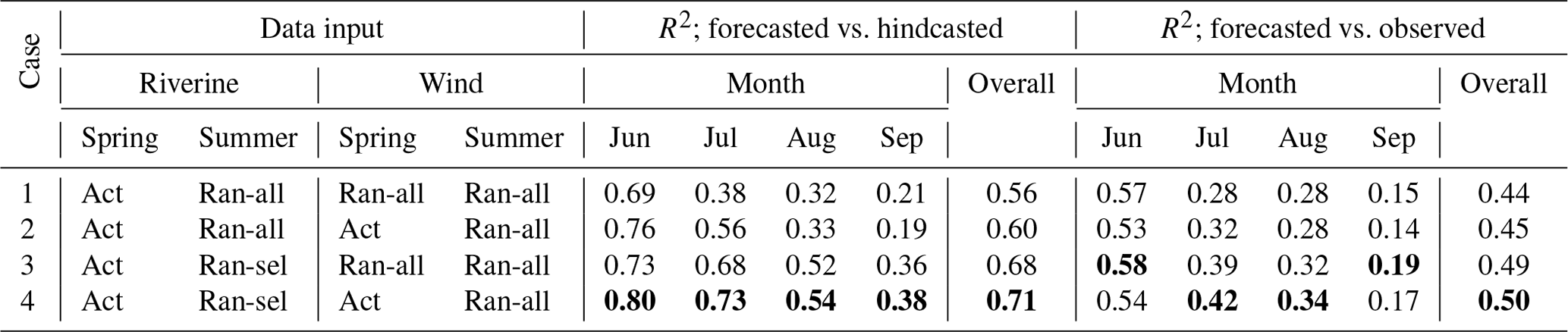
Table 2Explained variance (R2) in hindcasted and geostatistically observed HA by pseudo-forecasts based on the different data input cases. Here, the term Act indicates actual data for the specific year being forecasted are used, Ran-all indicates that input data are randomly sampled from the complete historical record, and Ran-sel indicates that riverine input data are randomly sampled from a subset of relevant historical years based on the regression projections for flow and loading. Spring includes March–May, while summer includes June–September records. The highest R2 values for each month are highlighted in bold.
3.3 Sensitivity to riverine and meteorological inputs
The results presented in the previous section are for the proposed forecasting approach with known spring loadings, discharge, and winds and with summer riverine inputs constrained through the regression projections (i.e., Case 4 in Sect. 2.5). In comparison, the more conventional Gulf forecasting approach, using known spring riverine inputs but with unknown wind and summer riverine inputs (i.e., randomly sampled from the entire historical record; Case 1) explains only around half of the variability in hindcasted and observed HA (i.e., 56 % and 44 %, respectively; Table 2). Also, the performance of Case 1 declines greatly from the beginning (June) to the end (September) of the summer. The inclusion of summer riverine records constrained through regression projections substantially increases the variance explained in both hindcasted and observed HA (Table 2; Cases 3 and 4). This improvement in performance is the most notable for July–September, indicating that the constrained summer inputs provide a more accurate determination of water column stratification and oxygen demand within the biophysical model. Additionally, the summer-wide average of the normalized IQR for Case 4 is, on average, 22 % lower than that of the conventional forecasting approach (Case 1).
The addition of actual spring wind data to the conventional approach (Table 2; Case 2) slightly increases the explained variance in hindcasted and observed HA by 4 % (i.e., from 56 % to 60 %) and 1 %, respectively. This forecast improvement is most notable in June and July because zonal wind velocities up to 3 months in advance regulate the transport of water and nutrients over the shelf (Obenour et al., 2015; Walker et al., 2005). Interestingly, about a quarter of the variability in hindcasted June HA remains unexplained, even when actual spring wind data are included (Table 2; Case 2). This is consistent with the importance of near-term wind and discharge inputs in controlling reaeration in the model. It is also consistent with the uncertainties presented in Fig. 6 and other modeling studies exploring the influence of wind on hypoxia formation (Forrest et al., 2011; Yu et al., 2015). Overall, the forecast is only moderately sensitive to the inclusion of actual spring wind velocities (compare Cases 1 to 2 and Cases 3 to 4). However, we anticipate that inclusion of actual spring wind data may still be important, especially for years with anomalous wind patterns.
Finally, for the preferred forecasting approach (Case 4) we examine an alternative way of determining the relevant years that constrain the distribution of riverine inputs for the forecast year. If only nitrogen loading regressions are used to constrain summer inputs (instead of both flow and loading regressions), the explained variability in the hindcasted total HA drops from 71 % (Table 2; Case 4) to 69 %. This relatively small drop in the predictive performance is not too surprising, as monthly nitrogen loading, which is the primary driver of many hypoxia models (Turner et al., 2006), is highly correlated with monthly discharge (r = 0.90). However, employing the discharge regressions (in addition to the loading regressions) better accounts for the influence of river flow on stratification and hypoxia formation (Obenour et al., 2012).
3.4 Implications for hypoxia forecasting and fisheries management
To our knowledge, there is only one hypoxia forecasting study (i.e., Laurent and Fennel, 2019) with a similar temporal scope to the current study. That study applied three-dimensional hydrodynamic–biogeochemical model hindcasts, which are weighted based on comparisons with historical May nitrogen loading only. Other predictive hypoxia studies have employed both discharge and wind (Forrest et al., 2011; Testa et al., 2017); however, they lacked the desired temporal resolution of this study. Here, we demonstrate how projections of summer riverine inputs based on spring discharge, loading, and watershed precipitation (Sect. 3.1) can be used to constrain model inputs, substantially improving hypoxia forecasting skill (Case 4; Table 2). We suggest that other hypoxia forecasting efforts could also benefit from such expanded and projected model inputs.
Our approach allows for daily forecasts of BWDO and HA for two shelf sections throughout the entire summer season. Generally, results indicate that HA can be forecasted up to 4 months ahead, but predictions for later months should be treated with increased caution given their higher uncertainties (Fig. 6). Note that the river input regressions only explain 25 %–30 % of the variability in August nitrogen loadings (Table 1), which is a major factor underlying the decrease in forecast skill in late summer. Additional sources of uncertainty in model inputs may arise from extreme climatic events (e.g., tropical storms and hurricanes), which are unpredictable at the forecasting timescales considered here. These storm events have a multifaceted effect on BWDO, potentially reaerating the bottom water column but also providing additional terrestrially derived or sediment-resuspended nutrients that may exacerbate hypoxia (Bianucci et al., 2018; Yu et al., 2015). Therefore, it is not surprising that the pseudo-forecast can explain only about one-third of the variability in hindcasted September total HA (Fig. 4). Overall, future hypoxia forecasting efforts would benefit from improvements in weather and riverine forecasting systems that provide more reliable projections for longer time periods.
The forecasts also explicitly distinguish between different sources of uncertainty in BWDO and HA (Fig. 5). Most previous forecasting studies for the northern Gulf (Forrest et al., 2011; Scavia et al., 2013; Turner et al., 2012), and other systems like Chesapeake Bay (Testa et al., 2017), implicitly represent uncertainty associated with unknown summer data inputs, sometimes accounting for it in the residual error. On the other hand, the recent study by Laurent and Fennel (2019) explicitly considers uncertainty due to stochastic summer riverine inputs but does not include parameter and residual error uncertainties in the generated forecasts. Thus, this study provides a more comprehensive uncertainty assessment and allows for management decisions that are robust to potential extremes (Keeney, 1982; Schuwirth et al., 2019).
Finally, the proposed approach has potential benefits for short- and long-term environmental planning and fisheries management. In the northern Gulf, the largest volume (Atlantic menhaden) and highest valued (Penaeid shrimp) fisheries occur during the summer months, concurrent with seasonal hypoxia. These fisheries are highly mobile, and hypoxia is known to affect the dynamics of both targeted species (Craig and Crowder, 2005; Craig and Bosman, 2013) and fishing fleets (Langseth et al., 2014; Purcell et al., 2017), with potential implications for the catch (Craig, 2012), economic conditions (Smith et al., 2017), and management (Langseth et al., 2016). However, previous attempts to correlate fishery performance (e.g., catch) with annual measures of hypoxic severity (e.g., area of hypoxia in late July) have had limited success (O'Connor and Whitall, 2007; Zimmerman and Nance, 2001) because neither the spatiotemporal dynamics of hypoxia or of the fishery have been considered. Thus, the proposed daily forecasts can potentially be linked to fisheries and ecosystem models (e.g., de Mutsert et al., 2016) to provide more actionable management guidance. In addition, while this study focuses on a 1 June forecast release date, consistent with current Gulf forecasting practices, future modeling enhancements might focus on updating the forecast over the summer as additional hydrometeorological data become available. Such updating could potentially benefit real-time, adaptive management of the fishery.
In this study, we demonstrate a novel approach for forecasting intraseasonal variability in BWDO and HA in the northern Gulf of Mexico by leveraging a Bayesian mechanistic model. This study generates the first daily hypoxia forecasts across the summer season (up to 4 months ahead), with a comprehensive uncertainty assessment. We show that the major sources of uncertainty include variability in data inputs and residual error, while model parameter uncertainty is relatively small. This study also compares how different methods for specifying riverine and meteorological model inputs influence forecast accuracy. In particular, we show how constraining summer riverine inputs based on spring conditions, including precipitation over the Mississippi River basin, can be used to improve the hypoxia forecasting skill. We also show that inclusion of monitored spring wind data further improves hypoxia forecasts. Together, these enhancements increase the retrospective pseudo-forecast accuracy from 44 % to 50 % (R2), while reducing forecast uncertainty by 22 % across summers, relative to the conventional approach using spring loadings and flows only (with randomly sampled summer riverine and spring–summer wind records). Thus, the forecasting system developed here provides an enhanced capacity to inform natural resources management in hypoxic coastal systems.
Model input data can be downloaded from the public repositories described in Sect. 2. Geostatistical estimates of BWDO are provided in Del Giudice et al. (2020).
The supplement related to this article is available online at: https://doi.org/10.5194/hess-26-1131-2022-supplement.
All authors designed the research, analyzed the results, and prepared the paper. AK developed the codes and created the tables and figures.
The contact author has declared that neither they nor their co-authors have any competing interests.
Publisher's note: Copernicus Publications remains neutral with regard to jurisdictional claims in published maps and institutional affiliations.
This article is part of the special issue “Frontiers in the application of Bayesian approaches in water quality modeling”. It is a result of the EGU General Assembly 2019, Vienna, Austria, 7–12 April 2019.
We thank Kevin Craig and the anonymous reviewers for their detailed comments on this paper. This work has been funded by the National Oceanic and Atmospheric Administration (grant no. NA16NOS4780203). This is NGOMEX contribution no. 260.
This research has been supported by the National Oceanic and Atmospheric Administration (grant no. NA16NOS4780203).
This paper was edited by Miriam Glendell and reviewed by three anonymous referees.
Benhamou, E.: A few properties of sample variance, arXiv: preprint, https://arxiv.org/abs/1809.03774 (last access: 1 November 2021), 2018.
Berrar, D.: Cross-Validation, in Encyclopedia of Bioinformatics and Computational Biology, Elsevier, 542–545, ISBN 9780128114322, 2019.
Bianchi, T. S., DiMarco, S. F., Cowan, J. H., Hetland, R. D., Chapman, P., Day, J. W., and Allison, M. A.: The science of hypoxia in the Northern Gulf of Mexico: A review, Sci. Total Environ., 408, 1471–1484, https://doi.org/10.1016/j.scitotenv.2009.11.047, 2010.
Bianucci, L., Balaguru, K., Smith, R. W., Leung, L. R., and Moriarty, J. M.: Contribution of hurricane-induced sediment resuspension to coastal oxygen dynamics, Sci. Rep.-UK, 8, 15740, https://doi.org/10.1038/s41598-018-33640-3, 2018.
Craig, J.: Aggregation on the edge: effects of hypoxia avoidance on the spatial distribution of brown shrimp and demersal fishes in the Northern Gulf of Mexico, Mar. Ecol. Prog. Ser., 445, 75–95, https://doi.org/10.3354/meps09437, 2012.
Craig, J. and Crowder, L.: Hypoxia-induced habitat shifts and energetic consequences in Atlantic croaker and brown shrimp on the Gulf of Mexico shelf, Mar. Ecol. Prog. Ser., 294, 79–94, https://doi.org/10.3354/meps294079, 2005.
Craig, J. K. and Bosman, S. H.: Small Spatial Scale Variation in Fish Assemblage Structure in the Vicinity of the Northwestern Gulf of Mexico Hypoxic Zone, Estuar. Coast., 36, 268–285, https://doi.org/10.1007/s12237-012-9577-9, 2013.
Del Giudice, D., Matli, V. R. R., and Obenour, D. R.: Bayesian mechanistic modeling characterizes Gulf of Mexico hypoxia: 1968–2016 and future scenarios, Ecol. Appl., 30, eap.2032, https://doi.org/10.1002/eap.2032, 2020.
de Mutsert, K., Steenbeek, J., Lewis, K., Buszowski, J., Cowan, J. H., and Christensen, V.: Exploring effects of hypoxia on fish and fisheries in the northern Gulf of Mexico using a dynamic spatially explicit ecosystem model, Ecol. Modell., 331, 142–150, https://doi.org/10.1016/j.ecolmodel.2015.10.013, 2016.
de Velasco, G. G. and Winant, C. D.: Seasonal patterns of wind stress and wind stress curl over the Gulf of Mexico, J. Geophys. Res.-Oceans, 101, 18127–18140, https://doi.org/10.1029/96JC01442, 1996.
Díaz, R. J. and Rosenberg, R.: Introduction to environmental and economic consequences of hypoxia, Int. J. Water Resour. D., 27, 71–82, https://doi.org/10.1080/07900627.2010.531379, 2011.
Donner, S. D. and Scavia, D.: How climate controls the flux of nitrogen by the Mississippi River and the development of hypoxia in the Gulf of Mexico, Limnol. Oceanogr., 52, 856–861, https://doi.org/10.4319/lo.2007.52.2.0856, 2007.
Faraway, J. J.: Linear Models with R, 2nd Edn., Taylor & Francis Group, ISBN 9781439887332, 2015.
Feng, Y., DiMarco, S. F., and Jackson, G. A.: Relative role of wind forcing and riverine nutrient input on the extent of hypoxia in the northern Gulf of Mexico, Geophys. Res. Lett., 39, L09601, https://doi.org/10.1029/2012GL051192, 2012.
Fennel, K., Hu, J., Laurent, A., Marta-Almeida, M., and Hetland, R.: Sensitivity of hypoxia predictions for the northern Gulf of Mexico to sediment oxygen consumption and model nesting, J. Geophys. Res.-Oceans, 118, 990–1002, https://doi.org/10.1002/jgrc.20077, 2013.
Fennel, K., Laurent, A., Hetland, R., Justić, D., Ko, D. S., Lehrter, J., Murrell, M., Wang, L., Yu, L., and Zhang, W.: Effects of model physics on hypoxia simulations for the northern Gulf of Mexico: A model intercomparison, J. Geophys. Res.-Oceans, 121, 5731–5750, https://doi.org/10.1002/2015JC011577, 2016.
Forrest, D. R., Hetland, R. D., and DiMarco, S. F.: Multivariable statistical regression models of the areal extent of hypoxia over the Texas–Louisiana continental shelf, Environ. Res. Lett., 6, 045002, https://doi.org/10.1088/1748-9326/6/4/045002, 2011.
Gentry, L. E., David, M. B., and McIsaac, G. F.: Variation in Riverine Nitrate Flux and Fall Nitrogen Fertilizer Application in East-Central Illinois, J. Environ. Qual., 43, 1467–1474, https://doi.org/10.2134/jeq2013.12.0499, 2014.
Greene, R. M., Lehrter, J. C., and Hagy III, J. D.: Multiple regression models for hindcasting and forecasting midsummer hypoxia in the Gulf of Mexico, Ecol. Appl., 19, 1161–1175, https://doi.org/10.1890/08-0035.1, 2009.
Hart, E. M. and Bell, K.: prism: Download data from the Oregon prism project, Zenodo, https://doi.org/10.5281/zenodo.33663, 2015.
Hetland, R. D.: Relating river plume structure to vertical mixing, J. Phys. Oceanogr., 35, 1667–1688, https://doi.org/10.1175/JPO2774.1, 2005.
Hinsby, K., Markager, S., Kronvang, B., Windolf, J., Sonnenborg, T. O., and Thorling, L.: Threshold values and management options for nutrients in a catchment of a temperate estuary with poor ecological status, Hydrol. Earth Syst. Sci., 16, 2663–2683, https://doi.org/10.5194/hess-16-2663-2012, 2012.
Justić, D. and Rose, K. A.: Modeling Coastal Hypoxia, edited by: D. Justic, K. A. Rose, R. D. Hetland, and K. Fennel, Springer International Publishing, Cham, 2017.
Justić, D. and Wang, L.: Assessing temporal and spatial variability of hypoxia over the inner Louisiana–upper Texas shelf: Application of an unstructured-grid three-dimensional coupled hydrodynamic-water quality model, Cont. Shelf Res., 72, 163–179, https://doi.org/10.1016/j.csr.2013.08.006, 2014.
Justić, D., Rabalais, N. N., and Turner, R. E.: Effects of climate change on hypoxia in coastal waters: A doubled CO2 scenario for the northern Gulf of Mexico, Limnol. Oceanogr., 41, 992–1003, https://doi.org/10.4319/lo.1996.41.5.0992, 1996.
Keeney, R. L.: Decision Analysis: An Overview, Oper. Res., 30, 803–838, https://doi.org/10.1287/opre.30.5.803, 1982.
Krug, E. C.: Coastal change and hypoxia in the northern Gulf of Mexico: Part I, Hydrol. Earth Syst. Sci., 11, 180–190, https://doi.org/10.5194/hess-11-180-2007, 2007.
Langseth, B. J., Purcell, K. M., Craig, J. K., Schueller, A. M., Smith, J. W., Shertzer, K. W., Creekmore, S., Rose, K. A., and Fennel, K.: Effect of Changes in Dissolved Oxygen Concentrations on the Spatial Dynamics of the Gulf Menhaden Fishery in the Northern Gulf of Mexico, Mar. Coast. Fish., 6, 223–234, https://doi.org/10.1080/19425120.2014.949017, 2014.
Langseth, B. J., Schueller, A. M., Shertzer, K. W., Craig, J. K., and Smith, J. W.: Management implications of temporally and spatially varying catchability for the Gulf of Mexico menhaden fishery, Fish. Res., 181, 186–197, https://doi.org/10.1016/j.fishres.2016.04.013, 2016.
Larson, L. W.: The great USA flood of 1993, IAHS Publ. Proc. Reports-Intern Assoc Hydrol. Sci., 239, 13–29, http://citeseerx.
ist.psu.edu/viewdoc/download?doi=10.1.1.595.3792&rep=rep1
&type=pdf (last access: 1 May 2020), 1997.
Laurent, A. and Fennel, K.: Time-Evolving, Spatially Explicit Forecasts of the Northern Gulf of Mexico Hypoxic Zone, Environ. Sci. Technol., 53, 14449–14458, https://doi.org/10.1021/acs.est.9b05790, 2019.
Le, C., Lehrter, J. C., Hu, C., and Obenour, D. R.: Satellite-based empirical models linking river plume dynamics with hypoxic area and volume, Geophys. Res. Lett., 43, 2693–2699, https://doi.org/10.1002/2015GL067521, 2016.
Lumley, T.: leaps: Regression Subset Selection. Based on Fortran code by Alan Miller, https://cran.r-project.org/package=leaps (last access: 1 May 2020), 2017.
Matli, V. R. R., Fang, S., Guinness, J., Rabalais, N. N., Craig, J. K., and Obenour, D. R.: Space-Time Geostatistical Assessment of Hypoxia in the Northern Gulf of Mexico, Environ. Sci. Technol., 52, 12484–12493, https://doi.org/10.1021/acs.est.8b03474, 2018.
Mattern, J. P., Fennel, K., and Dowd, M.: Sensitivity and uncertainty analysis of model hypoxia estimates for the Texas–Louisiana shelf, J. Geophys. Res.-Oceans, 118, 1316–1332, https://doi.org/10.1002/jgrc.20130, 2013.
Ménesguen, A. and Lacroix, G.: Modelling the marine eutrophication: A review, Sci. Total Environ., 636, 339–354, https://doi.org/10.1016/j.scitotenv.2018.04.183, 2018.
NDBC – National Data Buoy Center: https://www.ndbc.noaa.gov/, last access: 5 May 2019.
Obenour, D. R., Michalak, A. M., Zhou, Y., and Scavia, D.: Quantifying the Impacts of Stratification and Nutrient Loading on Hypoxia in the Northern Gulf of Mexico, Environ. Sci. Technol., 46, 5489–5496, https://doi.org/10.1021/es204481a, 2012.
Obenour, D. R., Michalak, A. M., and Scavia, D.: Assessing biophysical controls on Gulf of Mexico hypoxia through probabilistic modeling, Ecol. Appl., 25, 492–505, https://doi.org/10.1890/13-2257.1, 2015.
O'Connor, T. and Whitall, D.: Linking hypoxia to shrimp catch in the northern Gulf of Mexico, Mar. Pollut. Bull., 54, 460–463, https://doi.org/10.1016/j.marpolbul.2007.01.017, 2007.
Purcell, K. M., Craig, J. K., Nance, J. M., Smith, M. D., and Bennear, L. S.: Fleet behavior is responsive to a large-scale environmental disturbance: Hypoxia effects on the spatial dynamics of the northern Gulf of Mexico shrimp fishery, edited: by Xu, J., PLoS One, 12, e0183032, https://doi.org/10.1371/journal.pone.0183032, 2017.
Rabalais, N. N. and Turner, R. E.: Gulf of Mexico Hypoxia: Past, Present, and Future, Limnol. Oceanogr. Bull., 28, 117–124, https://doi.org/10.1002/lob.10351, 2019.
Rabalais, N. N., Turner, R. E., and Scavia, D.: Beyond science into policy: Gulf of Mexico hypoxia and the Mississippi River, Bioscience, 52, 129–142, https://doi.org/10.1641/0006-3568(2002)052[0129:BSIPGO]2.0.CO;2, 2002.
R Core Team: R: A Language and Environment for Statistical Computing, https://www.r-project.org/ (last access: 1 November 2021), 2019.
Reichert, P. and Borsuk, M. E.: Does high forecast uncertainty preclude effective decision support?, Environ. Modell. Softw., 20, 991–1001, 2005.
Scavia, D., Evans, M. A., and Obenour, D. R.: A Scenario and Forecast Model for Gulf of Mexico Hypoxic Area and Volume, Environ. Sci. Technol., 47, 10423–10428, https://doi.org/10.1021/es4025035, 2013.
Scavia, D., Bertani, I., Obenour, D. R., Turner, R. E., Forrest, D. R., and Katin, A.: Ensemble modeling informs hypoxia management in the northern Gulf of Mexico, P. Natl. Acad. Sci. USA, 114, 8823–8828, https://doi.org/10.1073/pnas.1705293114, 2017.
Schuwirth, N., Borgwardt, F., Domisch, S., Friedrichs, M., Kattwinkel, M., Kneis, D., Kuemmerlen, M., Langhans, S. D., Martínez-López, J., and Vermeiren, P.: How to make ecological models useful for environmental management, Ecol. Model., 411, 108784, https://doi.org/10.1016/j.ecolmodel.2019.108784, 2019.
Schwartz, M.: Boundary of Mississippi River Basin derived by dissolving WBD HU-4, https://www.sciencebase.gov/catalog/item/55de04d5e4b0518e354dfcf8 (last access: 1 May 2020), 2012.
Sinha, E. and Michalak, A. M.: Precipitation dominates interannual variability of riverine nitrogen loading across the continental United States, Environ. Sci. Technol., 50, 12874–12884, https://doi.org/10.1021/acs.est.6b04455, 2016.
Smith, M. D., Asche, F., Bennear, L. S., and Oglend, A.: Spatial-dynamics of Hypoxia and Fisheries: The Case of Gulf of Mexico Brown Shrimp, Mar. Resour. Econ., 29, 111–131, https://doi.org/10.1086/676826, 2014.
Smith, M. D., Oglend, A., Kirkpatrick, A. J., Asche, F., Bennear, L. S., Craig, J. K., and Nance, J. M.: Seafood prices reveal impacts of a major ecological disturbance, P. Natl. Acad. Sci. USA, 114, 1512–1517, https://doi.org/10.1073/pnas.1617948114, 2017.
Testa, J. M., Clark, J. B., Dennison, W. C., Donovan, E. C., Fisher, A. W., Ni, W., Parker, M., Scavia, D., Spitzer, S. E., Waldrop, A. M., Vargas, V. M. D., and Ziegler, G.: Ecological Forecasting and the Science of Hypoxia in Chesapeake Bay, Bioscience, 67, 614–626, https://doi.org/10.1093/biosci/bix048, 2017.
Thronson, A. and Quigg, A.: Fifty-Five Years of Fish Kills in Coastal Texas, Estuar. Coast., 31, 802–813, https://doi.org/10.1007/s12237-008-9056-5, 2008.
Turner, R. E., Rabalais, N. N., and Justic, D.: Predicting summer hypoxia in the northern Gulf of Mexico: Riverine N, P, and Si loading, Mar. Pollut. Bull., 52, 139–148, https://doi.org/10.1016/j.marpolbul.2005.08.012, 2006.
Turner, R. E., Rabalais, N. N., and Justic, D.: Gulf of Mexico Hypoxia: Alternate States and a Legacy, Environ. Sci. Technol., 42, 2323–2327, https://doi.org/10.1021/es071617k, 2008.
Turner, R. E., Rabalais, N. N., and Justić, D.: Predicting summer hypoxia in the northern Gulf of Mexico: Redux, Mar. Pollut. Bull., 64, 319–324, https://doi.org/10.1016/j.marpolbul.2011.11.008, 2012.
USACE: Atchafalaya and Mississippi River daily discharge, New Orleans Dist, https://www.mvn.usace.army.mil/Missions/Engineering/Stage-and-Hydrologic-Data/Historical-Discharges/, last access: 5 May 2019.
USGS: Streamflow and Nutrient Delivery to the Gulf of Mexico, https://toxics.usgs.gov/hypoxia/mississippi/flux_ests/delivery/index.html, last access: 5 May 2019.
Walker, N. D., Wiseman, W. J., Rouse, L. J., and Babin, A.: Effects of River Discharge, Wind Stress, and Slope Eddies on Circulation and the Satellite-Observed Structure of the Mississippi River Plume, J. Coast. Res., 216, 1228–1244, https://doi.org/10.2112/04-0347.1, 2005.
Yu, L., Fennel, K., and Laurent, A.: A modeling study of physical controls on hypoxia generation in the northern Gulf of Mexico, J. Geophys. Res.-Oceans, 120, 5019–5039, https://doi.org/10.1002/2014JC010634, 2015.
Zhang, F., Sun, Y. Q., Magnusson, L., Buizza, R., Lin, S.-J., Chen, J.-H., and Emanuel, K.: What Is the Predictability Limit of Midlatitude Weather?, J. Atmos. Sci., 76, 1077–1091, https://doi.org/10.1175/JAS-D-18-0269.1, 2019.
Zimmerman, R. J. and Nance, J. M.: Effects of hypoxia on the shrimp fishery of Louisiana and Texas, in: Coastal hypoxia: Consequences for living resources and ecosystems, edited by: Rabalais, N. N. and Turner, R. E., Coast. Estuar. Stud., 58, 293–310, 2001