The importance of vegetation in understanding terrestrial water storage variations

So far, various studies have aimed at decomposing the integrated terrestrial water storage variations observed by satellite gravimetry (GRACE, GRACE-FO) with the help of large-scale hydrological models. While the results of the storage decomposition depend on model structure, little attention has been given to the impact of the way that vegetation is represented in these models. Although vegetation structure and activity represent the crucial link between water, carbon, and energy cycles, their representation in large-scale hydrological models remains a major source of uncertainty. At the same time, the increasing availability and quality of Earth-observation-based vegetation data provide valuable information with good prospects for improving model simulations and gaining better insights into the role of vegetation within the global water cycle.

In this study, we use observation-based vegetation information such as vegetation indices and rooting depths for spatializing the parameters of a simple global hydrological model to define infiltration, root water uptake, and transpiration processes. The parameters are further constrained by considering observations of terrestrial water storage anomalies (TWS), soil moisture, evapotranspiration (ET) and gridded runoff (Q) estimates in a multi-criteria calibration approach. We assess the implications of including varying vegetation characteristics on the simulation results, with a particular focus on the partitioning between water storage components. To isolate the effect of vegetation, we compare a model experiment in which vegetation parameters vary in space and time to a baseline experiment in which all parameters are calibrated as static, globally uniform values.

Both experiments show good overall performance, but explicitly including varying vegetation data leads to even better performance and more physically plausible parameter values. The largest improvements regarding TWS and ET are seen in supply-limited (semi-arid) regions and in the tropics, whereas Q simulations improve mainly in northern latitudes. While the total fluxes and storages are similar, accounting for vegetation substantially changes the contributions of different soil water storage components to the TWS variations. This suggests an important role of the representation of vegetation in hydrological models for interpreting TWS variations. Our simulations further indicate a major effect of deeper moisture storages and groundwater–soil moisture–vegetation interactions as a key to understanding TWS variations. We highlight the need for further observations to identify the adequate model structure rather than only model parameters for a reasonable representation and interpretation of vegetation–water interactions.

1 Introduction

Since 2002, the Gravity Recovery and Climate Experiment (GRACE) mission has facilitated global monitoring of terrestrial water storage (TWS) variations from space – a milestone of global hydrology (Rodell, 2004; Famiglietti and Rodell, 2013). Observed TWS variations from GRACE have since become a cornerstone for diagnosing trends in water resources due to climate change or anthropogenic activities (Rodell et al., 2018; Reager et al., 2015; Scanlon et al., 2018; Syed et al., 2009; Tapley et al., 2019), as well as for benchmarking and improving global hydrological models (GHMs) (Scanlon et al., 2016; Döll et al., 2014; Werth et al., 2009; Zhang et al., 2017; Kumar et al., 2016; Eicker et al., 2014). Significant co-variations between GRACE TWS and the global land carbon sink (Humphrey et al., 2018) and surface temperatures (Humphrey et al., 2021) highlight the importance of the water cycle as the nexus in the Earth system.

However, GRACE TWS estimates represent a vertically integrated signal of all water stored in snow, ice, soil, surface water, and groundwater. Thus, understanding processes and mechanisms of TWS variations requires attribution of TWS variations to individual storage components. Despite advancements in remote sensing, large-scale quantification of these components based on observations remains challenging. For example, remote-sensing-based estimates of soil moisture only capture depths up to 5 cm and do not necessarily reflect the moisture availability in the deeper soil column (Dorigo et al., 2015). While these observations can be extrapolated to derive estimates of root zone moisture, either by using statistical relationships (Zhuang et al., 2020) or by data assimilation into land surface models (Reichle et al., 2017; Martens et al., 2017), such products rely on many assumptions. Therefore, GHMs have been necessary to interpret TWS variations in terms of contributions by snow, soil moisture, groundwater, or surface water. However, several studies suggested that current state-of-the-art GHMs cannot reproduce key patterns of observed TWS variations and show partly diverging TWS partitioning (Scanlon et al., 2018; Schellekens et al., 2017; Zhang et al., 2017; Kraft et al., 2021). This uncertainty of the available tools to interpret TWS variations is clearly a major obstacle for diagnosing and understanding global changes of the water cycle.

To improve model performance and reliability, GHMs are traditionally calibrated against measured discharge time series at the outlet of catchments (Müller Schmied et al., 2021; Telteu et al., 2021). However, discharge provides an integrated response of an entire catchment with very limited information on the interplay of different processes and spatial heterogeneities. In fact, the use of spatio-temporal data, for example, from remote sensing, has been suggested for model calibration (Su et al., 2020). While using spatio-temporal vegetation data, for example, the normalized difference vegetation index (NDVI) seemed promising for this at the catchment scale (Ruiz-Perez et al., 2017), many GHMs still have a limited usage of such data in their modelling approach. Some large-scale studies have shown clear improvements in model performance when a larger number of observational constraints are used to constrain the model parameters, especially when using TWS variations from GRACE (e.g. Lo et al., 2010; Rakovec et al., 2016; Bai et al., 2018; Mostafaie et al., 2018; Trautmann, 2018). Among them, Trautmann et al. (2018) contributed insights into the drivers of TWS variations across spatial and temporal scales in northern high latitudes, in particular with respect to contributions by snow vs. liquid water storages. In this study, we follow a similar framework of using multiple observational data streams to constrain a simple hydrological model to understand the role of varying vegetation characteristics for the partitioning of TWS components at the global scale.

Among liquid water storages, especially the differentiation between soil moisture and groundwater poses a challenge. Reflecting on the determinants of rather shallow soil moisture vs. deeper groundwater storage variations, it is apparent that under most conditions, the soil moisture state itself is the first-order control valve. In particular, it determines the amount of water that is available for soil water uptake for evapotranspiration but also for percolation into deeper soil layers and consequently recharge into the groundwater storage. The two key processes that shape soil moisture dynamics, infiltration and evapotranspiration (ET), are strongly mediated by the presence and properties of vegetation (Wang et al., 2018). For example, vegetation promotes infiltration over surface runoff due to larger surface roughness, dampened precipitation intensities, and more soil macropores due to rooting and biological activity. In fact, such roles of vegetation in a global climate model were already envisioned and evaluated almost 4 decades ago (Rind, 1984). In addition, vegetation alters soil properties like soil texture and organic matter content. Such soil properties together with rooting depth control the size of the soil moisture reservoir that is available for ET and how plants respond to drought stress conditions (Baldocchi et al., 2021; Yang et al., 2020). Furthermore, deep roots may connect to the groundwater and provide access to the deeper moisture storages and thus have wider implications on the hydrological cycle. Rooting depth is species-specific and, in addition, determined by the infiltration depth and groundwater table depth and thus has a high spatial heterogeneity both across the globe and at the local scale (Fan et al., 2017). The significance of interactions between vegetation and soil moisture is at the heart of ecohydrology (Rodriguez-Iturbe et al., 2001) and has become evident in many theoretical and experimental studies. Many studies analysed the effects of water availability on vegetation functioning (Porporato et al., 2004; Reyer et al., 2013; Wang et al., 2001; Yang et al., 2014) and the effect of changing vegetation cover on ecosystem water consumption (Du et al., 2021). While large-scale hydrologic models usually apply simplified and static vegetation characteristics (Quevedo et al., 2008; Weiss et al., 2012; Telteu et al., 2021), spatio-temporal variations of vegetation pattern are vital for good predictions of available water resources (Andersen et al., 2010). On the ecosystem scale, Xu et al. (2016) showed the advantage of accounting for different plant hydraulic traits in an ecosystem model. And on a global scale, Weiss et al. (2012), for instance, showed the positive influence on modelled evaporation when static vegetation characteristics are replaced by monthly LAI (leaf area index) estimates in a climate model. However, how the representation of vegetation affects global water storages and in particular the partitioning of TWS in large-scale hydrological models has received surprisingly little attention so far.

Therefore, the objective of this study is to investigate the effect of vegetation-dependent parameterizations of key hydrological processes on TWS partitioning at the global scale using a multi-criteria model data fusion approach. The model, an expanded version of Trautmann et al. (2018), is a simple conceptual four-pool water balance model. Model parameters are calibrated against TWS variations from GRACE (Wiese et al., 2018), ET from FLUXCOM (Jung et al., 2019), runoff from GRUN (Ghiggi et al., 2019), and ESA CCI soil moisture (Dorigo et al., 2017). We contrast two experiments which differ only with respect to how vegetation-related parameters are defined: (1) a baseline experiment with global uniform parameters and (2) a vegetation experiment where vegetation parameters vary in space and partly in time. In contrast to the traditional approach of spatializing vegetation parameters by plant functional type or land cover class, and keeping this a priori parameterization fixed during model application, we take advantage of continuous information on few key properties that link vegetation and hydrological processes: (1) spatially distributed and time-varying active vegetation cover that influences transpiration demand and interception storage, (2) the spatial pattern of soil water supply for transpiration via roots, and (3) the spatially distributed and time-varying influence of vegetation cover on infiltration and runoff generation. Specifically, we are addressing the following questions:

• 1.

  Where, when, and by how much are global hydrological simulations improved by spatially distributed and time-varying vegetation parameters?

• 2.

  To what extent do the attribution and interpretation of TWS variations for individual storage components change when introducing spatial and temporal variation of vegetation parameters?

2 Methods

In the first section, we give a general overview on the design of this study. Subsequently, the model and data streams used as well as the calibration and evaluation approach are explained in more detail.

2.1 Overview

To assess the potential effect of including continuous information on vegetation, we compare two model variants that are based on the same conceptual structure: (1) a base model with static, globally uniform parameter values (B) and (2) a model variant that includes spatially (and temporally) varying vegetation characteristics by defining vegetation parameters as a function of global data products (VEG). We additionally performed an experiment that discretizes vegetation parameters for distinct classes of plant functional types, similarly to some other GHMs. This PFT experiment is explained and shown in Sect. S9 in the Supplement.

Forced with global climate data, the parameters of each variant are calibrated for a spatial subset against multiple Earth-observation-based data. In the B experiment, the parameters themselves are calibrated, and globally constant parameter values are obtained. While the optimized parameters implicitly account for the effect of the nearly ubiquitous presence of vegetation, they cannot represent effects of spatially and/or temporally varying vegetation properties. In the VEG experiment, we describe vegetation-related parameters as a linear function of spatio-temporal varying vegetation variables; i.e. we calibrate scalars representing the slopes of these functions. By calibrating the slope, we include the continuous pattern from the data but scale it to best fit the observational constraints. Hence, vegetation-related parameters vary explicitly spatially and partly temporally.

Once the parameters are calibrated, the simulations for the whole domain (global) are used to evaluate the model performance at different spatial and temporal scales. To finally delineate the effect of including varying vegetation characteristics on the composition of simulated TWS across temporal (mean seasonal, inter-annual) and spatial (local grid scale, spatially aggregated) scales, we use the impact index as defined by Getirana et al. (2017).

The model is run on daily time steps at a $\mathrm{1}{}^{\circ }\times \mathrm{1}{}^{\circ }$ latitude/longitude resolution, focusing on vegetated regions under primarily natural conditions. To avoid biases of the calibrated model parameters due to processes that are not represented in the model structure, we exclude grid cells with >10 % permanent snow and ice cover, >50 % water fraction, >20 % bare land surface, and >10 % artificial land cover fraction. These grid cells are masked out using the GlobeLand30 fractional land-cover map v2 (Chen et al., 2014). Additionally, we exclude regions with a large human influence, mainly related to groundwater extraction, on the trend in GRACE TWS variations (Rodell et al., 2018) (see Fig. 2). The final study area comprises 74 % of the global land area. All other datasets used in this study were resampled to the $\mathrm{1}{}^{\circ }\times \mathrm{1}{}^{\circ }$ grid and subset to the same grid cells.

Due to the temporal coverage of forcing data and observational constraints, we calibrate the model for the period January 2002–December 2014, while the global-scale model runs and analyses are performed for the period March 2000–December 2014. Prior to each model run, all states are initialized by a 8-year spin-up period. The forcing for the spin-up period is assembled by randomly rearranging complete years of the forcing data.

2.2 Model description

The conceptual hydrological model is forced by daily precipitation, air temperature, and net radiation (Table 1). It includes a snow component (see Trautmann et al., 2018), a two-layer soil water storage (wSoil), a deep soil water storage (wDeep), and a delayed, slow water storage (wSlow). The schematic structure of the model is shown in Fig. 1, and calibration parameters are explained in Table 2.

Table 1 Data used for model forcing, for description of vegetation characteristics, and for model calibration.

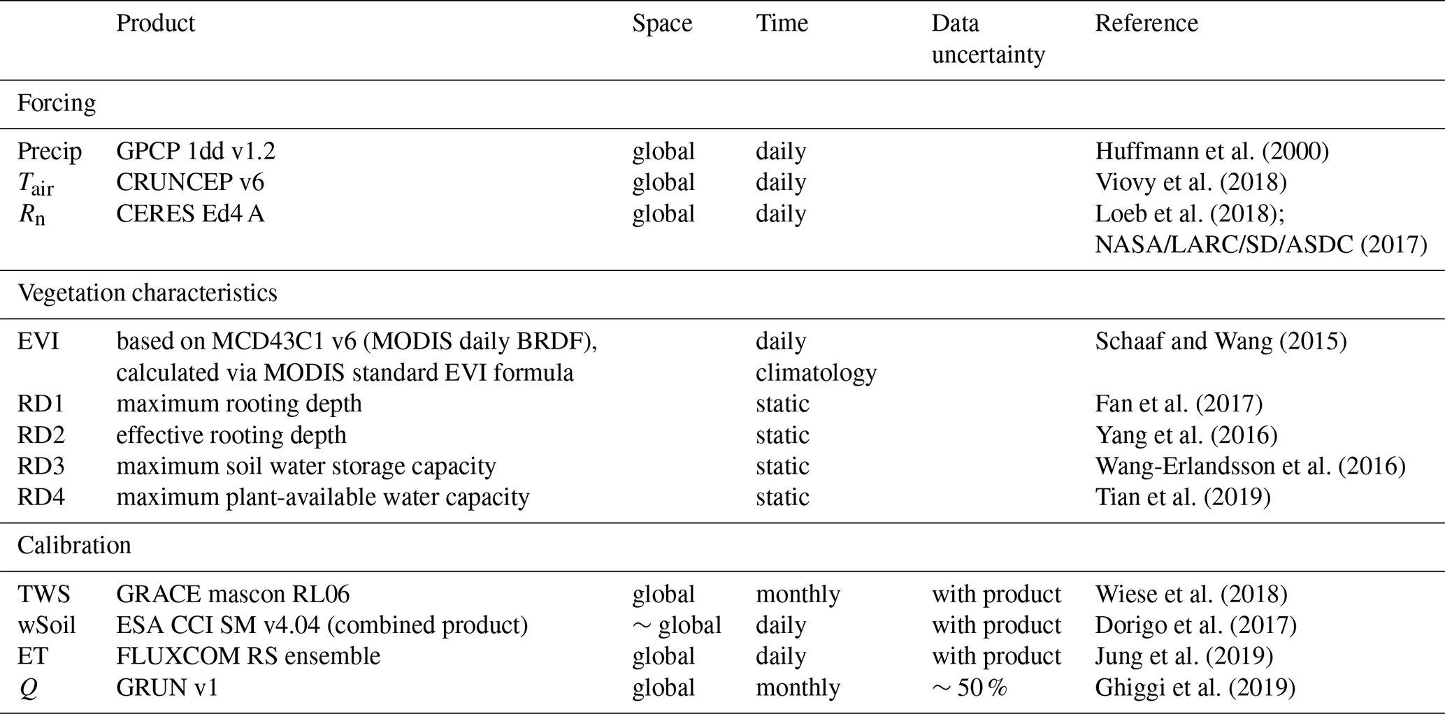
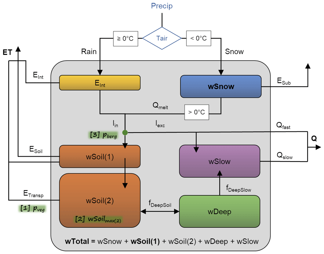
Figure 1 Schematic of the underlying model structure, with blue font denoting forcing data: Precip is precipitation, and T_air is air temperature. Boxes represent states as follows: E_int is interception storage, wSnow snow water storage, wSoil(1) upper soil layer, wSoil(2) second soil layer, wDeep deep water storage, and wSlow slowly varying water storage. Arrows denote fluxes as follows: Rain is rainfall, Snow snowfall, E_Sub sublimation, Q_melt snowmelt, I_in incoming water from throughfall and snowmelt, I_exc infiltration excess, Q_fast fast direct runoff, Q_slow slow runoff, Q total runoff, E_Int evaporation from interception storage, E_Soil soil evaporation, E_Transp plant transpiration, ET total evapotranspiration, f_DeepSoil the flux between wSoil and wDeep (percolation resp. capillary rise), and f_DeepSlow the flux from wDeep to wSlow. Bold print highlights model variables that are constrained in the calibration. Green highlights show where vegetation influence is included explicitly: [1] the parameter p_veg to define each grid cell's vegetation fraction, [2] the parameter wSoil_max(2) that defines the maximum plant-available soil water, and [3] the parameter p_berg to define the infiltration and runoff generation partitioning.

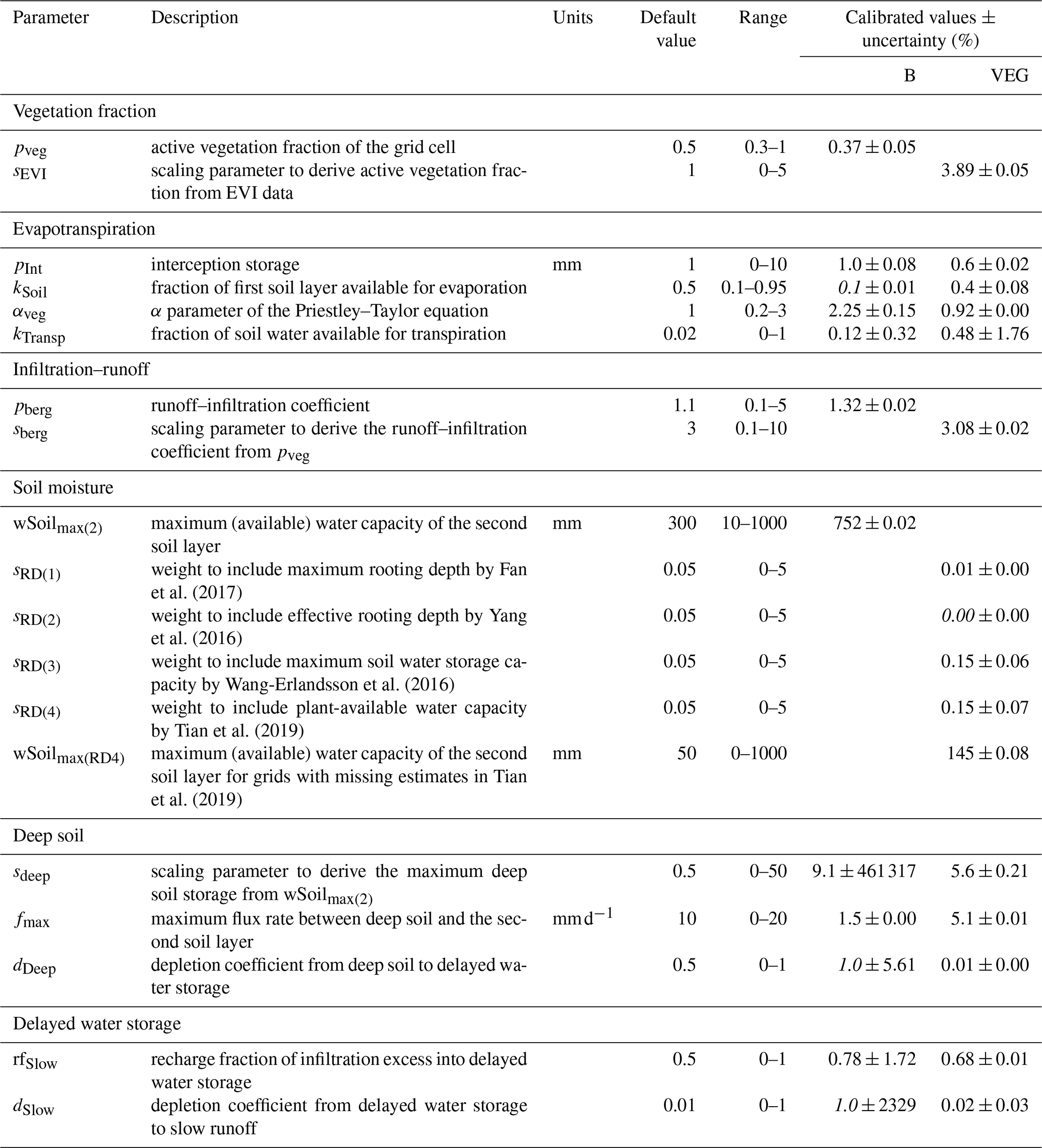
Table 2 Calibrated model parameters and their description, range, and calibrated values for experiments B and VEG. Text in italics highlights calibrated values at the predefined parameter bounds.

Depending on air temperature (T_air), precipitation (Precip) is partitioned into snowfall (Snow), that accumulates in the snow storage (wSnow), and rainfall (Rain), that is partly retained in an interception storage. Interception throughfall together with snowmelt is partitioned into infiltration and infiltration excess depending on the ratio of actual soil moisture and maximum soil water capacity following Bergström (1991):

$$\begin{array}{}\text{(1)}& I_{\text{exc}}=I_{\text{in}}{\left[{\displaystyle \frac{{\sum }_{l=\mathrm{1}}^{\mathrm{2}}\text{wSoil}\left(l\right)}{{\sum }_{l=\mathrm{1}}^{\mathrm{2}}{\text{wSoil}}_{\text{max}\left(l\right)}}}\right]}^{p_{\text{berg}}},\end{array}$$

where I_exc is the infiltration excess, I_In is the incoming water from throughfall and snowmelt, wSoil(l) is the soil moisture and wSoil_max(l) the maximum soil water capacity of each soil layer l, and p_berg is a calibration parameter. While p_berg<1 allocates a small fraction of the incoming water to the soil water pool even if it is nearly empty, p_berg>1 allows a large fraction of incoming water to infiltrate into the soil when soil saturation is already high, and p_berg=1 describes a linear relationship between soil water saturation and the amount of incoming water that infiltrates.

A fraction of the infiltration excess (defined by the global calibration parameter rf_Slow) then replenishes a delayed water storage (wSlow) that acts as a linear reservoir and generates slow runoff (Q_slow). The remaining infiltration excess represents fast direct runoff (Q_fast). Q_fast and Q_slow together represent total runoff Q that flows out of the system, i.e. grid cell.

Infiltrated water is distributed among two soil layers following a top-to-bottom approach, where the maximum capacity of the first soil layer is prescribed as 4 mm, in order to match the tentative depth of satellite soil moisture observations, while the storage capacity of the second soil layer is a calibration parameter (wSoil_max(2)). The second soil layer is connected with a deeper water storage (wDeep). The size of wDeep is defined as a multiple of wSoil_max(2) by the calibrated scaling parameter s_deep. Depending on the moisture gradient between the two storages, water either percolates from the second soil layer to the deeper soil, or it rises from the deeper storage into the second soil layer, by scaling to a maximum flux rate (defined by the global calibration parameter, f_max). The deeper storage therefore acts as a storage buffer that linearly discharges further to the delayed water storage (wSlow), which also receives part of the infiltration excess.

Evapotranspiration (ET) is represented by a demand–supply approach that is driven by a potential ET demand following Priestley–Taylor and is limited by the available soil moisture supply. ET is partitioned into interception evaporation (E_Int), bare soil evaporation from the first soil layer (E_Soil), and plant transpiration from the two soil layers (E_Transp). Interception and plant transpiration are only calculated for the vegetated fraction of each grid cell, while bare soil evaporation is limited to the non-vegetated fraction of each grid cell.

While water in wSoil is directly available for ET, wDeep is only indirectly accessible by capillary rise, and the water stored in wSlow is not plant-accessible. Total water storage is the sum of all water storages, including wSnow, wSoil, wDeep, and wSlow. Although groundwater and surface water storages are not implemented explicitly, they are effectively included in wDeep and wSlow, especially after calibration of associated storage parameters against GRACE TWS.

2.3 Vegetation characteristics

We include three aspects of vegetation influence on hydrological processes: (1) the specific transpiration demand by vegetation, (2) the soil water supply for transpiration via roots, and (3) the influence of vegetation on infiltration and runoff generation. These three aspects are controlled by three corresponding model parameters, namely the grid cell's vegetation fraction (p_veg), the maximum plant-available soil water (wSoil_max(2)), and the runoff generation–infiltration coefficient (p_berg). In the VEG experiment, scalar parameters are used as linear multipliers of observation-based spatio-temporal patterns to harvest the information of spatial and temporal patterns from the continuous data products.

2.3.1 Vegetation fraction

The parameter p_veg reflects the vegetation cover of each grid cell that influences the grid's interception storage, transpiration demand, and partitioning of evapotranspiration components. To describe its spatial and seasonal variations, we include the mean seasonal cycle (MSC) of the Enhanced Vegetation Index (EVI). Therefore, p_veg at each time step is defined as a linear function of EVI, where s_EVI is the calibrated scaling parameter:

$$\begin{array}{}\text{(2)}& p_{\text{veg}}=s_{\text{EVI}}\cdot \text{EVI},\end{array}$$

with $\mathrm{0}\le p_{\text{veg}}\le \mathrm{1}$.

EVI data are calculated via the MODIS standard formula (Didan and Barreto-Munoz, 2019) using the daily BRDF, nadir BRDF-adjusted reflectance values MCD43C1 v6 (Schaaf and Wang, 2015) for the period January 2001–December 2014:

$$\begin{array}{}\text{(3)}& \text{EVI}=\mathrm{2.5}{\displaystyle \frac{\text{NIR–red}}{\text{NIR}+\mathrm{6}\cdot \text{red}-\mathrm{7.5}\cdot \text{blue}+\mathrm{1}}}.\end{array}$$

Since the daily EVI time series are not continuous due to noise and missing values during cloudy conditions, snow, and darkness, the data were preprocessed to be used in the model. For each grid cell, we calculate the median seasonal cycle, fill long gaps during wintertime with a low value, interpolate missing values, and smooth the time series. Therefore, winter is defined as days with negative net radiation, and gaps are considered long when 10 consecutive days of EVI data are missing. The wintertime gaps are filled with the 5th percentile of available wintertime data. The remaining missing values are linearly interpolated, and finally the resulting seasonal cycle is smoothed by a local regression with weighted linear least squares and a first-order polynomial model.

2.3.2 Plant-available soil water

In order to determine the soil water supply for transpiration as a function of vegetation, we define the maximum soil water capacity of the second soil layer wSoil_max(2) based on rooting depth and soil water storage capacity data. We include the maximum rooting depth by Fan et al. (2017) (RD1), effective rooting depth by Yang et al. (2016) (RD2), maximum soil water capacity by Wang-Erlandsson et al. (2016) (RD3), and maximum plant-accessible water capacity by Tian et al. (2019) (RD4). Due to our definition of wSoil_max(2) as maximum plant-accessible water, all four data are, theoretically, suitable when focusing on spatial patterns. Practically, though, they vary in their definition, underlying approaches, spatial coverage and derived spatial pattern. The RD1 and RD2 are based on principles of vegetation optimality and plant adaptation, and RD3 and RD4 are based on a water balance perspective but using Earth observations and/or data assimilation techniques. Therefore, we employ an approach in which we obtain a linear combination of the four products where the weights of each product are calibrated during the multi-criteria parameter optimization:

$$\begin{array}{}\text{(4)}& {\text{wSoil}}_{\text{max(2)}}={\sum }_{d=\mathrm{1}}^{\mathrm{4}}{s}_{\text{RD}\left(d\right)}\cdot \text{RD}\left(d\right),\end{array}$$

where RD(d) is the data from each data stream d, and s_RD(d) denotes the corresponding scaling factors that are calibrated. As RD4 from Tian et al. (2019) is only available for arid to moderately humid vegetated land area and excludes tropical forests (Tian et al., 2019), resulting gaps in the study area are filled by the calibration parameter wSoil_max(RD4) prior to scaling RD4.

2.3.3 Runoff/infiltration coefficient

Finally, vegetation structure also affects the infiltration and runoff generation process as it alters the surface and sub-surface characteristics. To reflect this influence, we describe the infiltration–runoff parameter p_berg (Eq. 1) as a linear function of the vegetation fraction p_veg:

$$\begin{array}{}\text{(5)}& p_{\text{berg}}=s_{\text{berg}}\cdot p_{\text{veg}},\end{array}$$

where s_berg is the calibrated scaling parameter.

2.4 Model calibration

In order to keep computational costs low and to avoid overfitting of model parameters, we perform model calibration for a subset of 904 (8 %) grid cells. Since model parameters are expected to vary much more in space than in time (between years), and due to the rather short time period of available constraints, we build two subsets of data for calibration and validation data in the spatial domain rather than in time (spatial split-sample approach). Calibration grid cells are chosen by a stratified random sampling method that maintains the overall proportion of different climate and hydrological regimes defined by Köppen–Geiger climate regions (Kottek et al., 2006).

Since this study focuses on the impact of vegetation, and in order to keep the number of calibration parameters low, we do not optimize snow-related parameters and use the optimized snow parameters from Trautmann et al. (2018). This results in a total of 11 calibration parameters for the B model and a total of 16 parameters for the VEG model (Table 2).

In order to constrain different aspects of the water cycle, we use a multi-criteria calibration approach similar to Trautmann et al. (2018). The parameters of each model variant are simultaneously optimized against multiple observational constraints, including monthly TWS anomalies from GRACE (Wiese et al., 2018; Watkins et al,. 2015), ESA CCI soil moisture (Dorigo et al., 2017), evapotranspiration estimates from the FLUXCOM-RS ensemble (Jung et al., 2019), and gridded runoff from GRUN (Ghiggi et al., 2019) (Table 1).

When using observational datasets from several sources, it is essential to consider possible inconsistencies between them that arise from their respective characteristics and uncertainties (Zeng et al., 2015, 2019). Therefore, we derived the monthly water (im)balance of the observations following a similar approach to Rodell et al. (2015) (see Sect. S10 in the Supplement). Although we did not find major systematic inconsistencies at the global scale, we take into account each dataset's characteristics and uncertainties in model calibration via the cost term at the grid cell level. To this end, we only use grid cells and time steps with available observations, which vary for the different data streams. To retrieve one cost term per observational constraint, we concatenate the time series of all grid cells into a single vector for which costs are calculated. The individual cost terms are considered to have the full weight of 1, resulting in a total cost value (cost_total) as the sum of individual costs. The total cost is then minimized during the optimization process using a global search algorithm, the covariance matrix evolutionary strategy (CMAES) algorithm (Hansen and Kern, 2004).

$$\begin{array}{}\text{(6)}& {\text{cost}}_{\text{total}}={\sum }_{\text{ds}=\mathrm{1}}^n\text{cost(ds)},\end{array}$$

where cost(ds) is the cost for each data stream ds. For TWS, ET, and Q, the cost terms are based on the weighted Nash–Sutcliffe efficiency (Nash and Sutcliffe, 1970), which explicitly considers the observational uncertainty σ:

$$\begin{array}{}\text{(7)}& \text{cost}={\displaystyle \frac{{\sum }_{i=\mathrm{1}}^n\frac{(x_{\text{obs},i}-x_{\text{mod},i}{)}^{\mathrm{2}}}{{\mathit{\sigma }}_i}}{{\sum }_{i=\mathrm{1}}^n\frac{(x_{\text{obs},i}-{\stackrel{\mathrm{‾}}{x}}_{\text{obs}}{)}^{\mathrm{2}}}{{\mathit{\sigma }}_i}}},\end{array}$$

where x_mod,i is the modelled variable, x_obs,i is the observed variable, ${\stackrel{\mathrm{‾}}{x}}_{\text{obs}}$ is the average of x_obs, and σ_i is the uncertainty of x_obs of each data point i. The cost criterion reflects the overall fit in terms of variances and biases, with an optimal value of 0 and a range from 0–∞.

Owing to the larger uncertainties of Q_obs on inter-annual scales (Ghiggi et al., 2019), we only use the monthly mean seasonal cycle, while for the other variables, full monthly time series were used.

To define σ of ET_obs, we utilize the median absolute deviation of the FLUXCOM-RS ensemble. For Q_obs, we assume an average uncertainty of 50 % based on values reported in Ghiggi et al. (2019). For TWS_obs, the spatially and temporally varying uncertainty information provided with the GRACE data is used. In addition, the largest monthly values of TWS_obs ($<-\mathrm{500}$ and >500 mm) were masked out to avoid the effect of outliers on optimization results. Note that these outliers represent less than 0.5 % of the data and are mainly located in coastal arctic regions and are, thus, potentially related to land and sea ice and/or leakage from neighbouring grid cells over ocean. Before calculating cost_TWS, the monthly means of observed and modelled TWS are respectively removed to calculate anomalies over a common time period 1 January 2002–31 December 2012.

Since remote-sensing-based soil moisture only captures the top few centimetres of soil depth, usually about 5 cm, cost_wSoil is calculated based on the modelled soil moisture in the first soil layer. As the combined ESA CCI soil moisture imposes absolute values and ranges from GLDAS Noah (Dorigo et al., 2015), we use Pearson's correlation coefficient as cost_wSoil and focus on soil moisture dynamics that is most reflective of the original remote sensing observation. Only estimates from 1 January 2007 onwards are considered, as data before that period are sparse. Further, cost_wSoil is calculated from the monthly averaged values to circumvent the large noise in the daily data. Thereby, only months with observations available for at least 10 d are considered. Due to snow cover, the temporal coverage of the product decreases with increasing latitude. Therefore, to prevent a bias towards northern summer months, we also exclude grid cells that lack more than 40 % of monthly estimates. After filtering for missing data, monthly surface soil moisture time series for 56 % of the total study area and 51 % of the calibration grid cells are available.

2.5 Model evaluation and analysis

For model evaluation, we contrast the optimized parameter values and their uncertainties. The relative uncertainty in the optimized parameter vector is estimated by quantifying each parameter's standard error according to Omlin and Reichert (1999) and Draper and Smith (1981), similar to Trautmann et al. (2018).

For each experiment, the optimized parameter sets are used to produce model simulations for the global study area. Their performances are then evaluated using Pearson's correlation coefficient and the uncertainty-weighted Nash–Sutcliffe efficiency (wNSE) for TWS, ET, and Q observations (Eq. 8). The performances are evaluated on local (for each grid cell individually), regional, and global scales.

$$\begin{array}{}\text{(8)}& \text{wNSE}=\mathrm{1}-{\displaystyle \frac{{\sum }_{i=\mathrm{1}}^n\frac{(x_{\text{obs},i}-x_{\text{mod},i}{)}^{\mathrm{2}}}{{\mathit{\sigma }}_i}}{{\sum }_{i=\mathrm{1}}^n\frac{(x_{\text{obs},i}-{\stackrel{\mathrm{‾}}{x}}_{\text{obs}}{)}^{\mathrm{2}}}{{\mathit{\sigma }}_i}}}\end{array}$$

For the regional analysis, we derive five hydroclimatic regions by performing a cluster analysis using the spatio-temporal characteristics of TWS, ET, and Q observations, as well as each grid cell's latitude. By that, each zone is characterized by similar seasonal dynamics and amplitudes of the water cycle variables, allowing for a better comparison of regional averages than, for example, the commonly used Köppen–Geiger regions which lump regions with very different amplitudes and phasing of the water cycle variables. The resulting regions are shown in Fig. 2. Region 1 comprises the snow-dominated northern latitudes (cold), while region 2 includes the moderate mid-latitudes (temperate). Very humid and mostly tropical regions are combined in region 3 (humid). Region 4 is characterized by a distinct rain season (sub-humid), while region 5 includes semi-arid areas in low latitudes (semi-arid). Although we hereafter use these hydroclimatic cluster regions for model evaluation, the same analysis for Köppen–Geiger climate zones is presented in Fig. S11 in the Supplement to facilitate comparison with other studies.

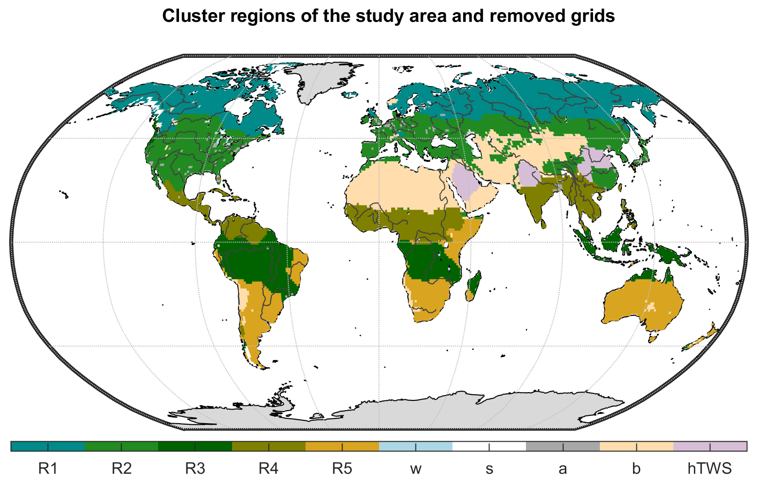
Figure 2 Hydroclimatic cluster regions of the study area (R1 – cold, R2 – temperate, R3 – humid, R4 – sub-humid, R5 – semi-arid) and grid cells that have been excluded from this study (w is the water fraction >50 %, s the permanent snow and ice cover >10 %, a the artificial land cover fraction >10 %, b the bare land surface >20 %, and hTWS the direct human impact on the trend in GRACE TWS).

Finally, we assess the contributions of the four water storage components, wSnow, wSoil, wDeep and wSlow, to seasonal and inter-annual variations of the total water storage across spatial scales, i.e. the local grid cell, the regional and the global average. To do so, we apply the impact index I following Getirana et al. (2017). The metric describes the contribution C of each water storage s as the sum of its absolute monthly anomaly:

$$\begin{array}{}\text{(9)}& C_s={\sum }_{t=\mathrm{1}}^{\mathit{\text{nt}}}\mathrm{|}{s}_t-\stackrel{\mathrm{‾}}{s}\mathrm{|},\end{array}$$

where $\stackrel{\mathrm{‾}}{s}$ is the average storage of the time steps t–nt, with nt=12 for mean seasonal and nt=178 for inter-annual dynamics.

The impact index I_s is then defined as the ratio of each water storage component contribution C_s to the total contributions from all storage components:

$$\begin{array}{}\text{(10)}& I_s={\displaystyle \frac{C_s}{{\sum }_{s=\mathrm{1}}^n{C}_s}}.\end{array}$$

The value of I_s range from 0–1, with 0 indicating no impact and 1 indicating full control of all variations.

3 Results

In the following section we first evaluate both calibrated model variants by comparing their calibrated model parameters and by comparing modelled TWS, ET and Q against observations at global, regional and local scale. Subsequently, we show the contribution of individual storage components to TWS variability for B and VEG on different spatial and temporal scales.

3.1 Model evaluation

3.1.1 Calibrated parameters

Table 2 summarizes the calibrated parameters and their uncertainties for the B and VEG model experiments. Overall, including varying vegetation characteristics leads to more plausible parameter values after calibration, while in B several parameters hit their prescribed bounds. Furthermore, very high parameter uncertainties present in B, that indicate poorly constrained values, could be strongly reduced in VEG (Fig. S3 in the Supplement).

For B, p_veg suggests that on average only 37 % of each grid cell is covered with vegetation globally. This low vegetation fraction is counteracted by a high α_veg value (2.25), which is much higher than commonly used α coefficients of the Priestley–Taylor equation of around 1.2 (Lu et al., 2005), to yield good performance of modelled ET (Fig. 3). At the same time, a very low fraction of the first soil layer is available for soil evaporation, as k_Soil hits its lower bound of 10 %. In addition, the parameters controlling the drainage from deep and slow water storage (d_Deep, d_Slow) are high, resulting in a fast drainage and effectively discarding any influence of these water pools.

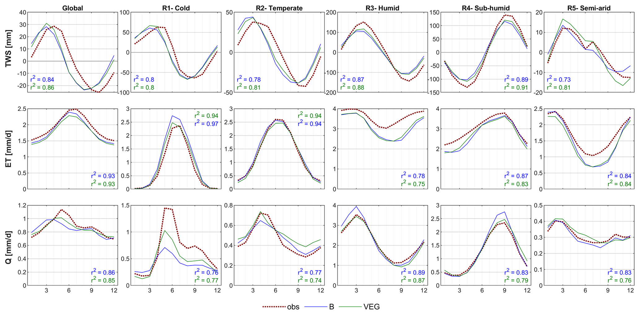
Figure 3 Global and regional mean seasonal cycles of total water storage (TWS), evapotranspiration (ET), and runoff (Q) for the B and VEG experiments compared to the observational constraints by GRACE (TWS), FLUXCOM (ET), and GRUN (Q).

For VEG, the median vegetation fraction is 73 %, leading to a more realistic fraction of soil moisture being available for evaporation (k_Soil=0.4), which is similar to the modal value of 0.33 reported by McColl et al. (2017), and a more realistic α_veg value of 0.92, that effectively leads to the median Priestley–Taylor α coefficient of 0.81 (Fig. S2 in the Supplement). In comparison to B, the resulting wSoil_max(2) of VEG with a median value of 52 mm is considerably lower. Its spatial pattern mainly originates from RD3 (Wang-Erlandsson et al., 2016) and RD4 (Tian et al., 2019) data, while RD1 (Fan et al., 2017) contributes only little, and RD2 (Yang et al., 2016) data are negligible. The resulting spatial patterns of the maximum soil water capacity from the combination of all datasets (Sect. S2) are still consistent with those from other estimates and patterns of rooting depth (e.g. Schenk and Jackson, 2005). We note here that the soil water capacity data are favoured over the rooting depth data. This agrees with Küçük et al. (2022), who suggest that estimating plant storage capacity based on Earth observation data may be more suitable than those using optimality principles. Related to the limited size of wSoil, calibration enforces a deeper and a slow water storage with reasonable depletion parameters (d_Deep, d_Slow) in order to match observed TWS variations. By that, the considerable low wSoil_max(2) parameter is counteracted by refilling wDeep, which indirectly provides plant-accessible water via capillary rise. Likewise, k_Transp, which describes the fraction of the second soil layer that is available for transpiration, is relatively high, as a larger fraction of the small soil water storage needs to transpire to match observed ET. Hence, calibrated k_Transp is higher than empirical values of ET decay between 0.02–0.08 that are based on assuming one soil water pool (Teuling et al., 2006).

3.1.2 Model performance

Table 3 contrasts the overall model performance metrics for TWS, ET, and Q for the two experiments for the calibration subset of 8 % grid cells (opti) and the entire study domain (global). The metrics are calculated in the same way as during optimization, i.e. by concatenation of the time series of all grid cells into a single vector for which statistics are calculated. In general, the differences between opti and global, as well as between B and VEG, are marginal. For VEG, results mainly improve for TWS and slightly for ET. Although the models were only calibrated for the spatial subset in opti, equally good or even better performances are obtained when the calibrated parameters are applied over the entire study domain. This suggests that the calibration subset was representative of the entire study domain, and the calibration did not overfit model parameters.

Table 3 Overall model performance metrics in terms of weighted Nash–Sutcliffe efficiency (wNSE) and Pearson's correlation coefficient (corr) of total water storage (TWS), evapotranspiration (ET), and runoff (Q) in B and VEG experiments for the calibration subset (opti) and the entire study domain (global).

Among the variables, the best model performance in terms of wNSE and corr is obtained for ET. While the correlation between observed and simulated TWS is high, the overall wNSE is relatively low, which mainly results from higher uncertainties in TWS_obs and a larger variance error, likely originating from grid cells with low observed TWS variance.

Similar to the global metrics, the average mean seasonal cycle of different regions shows an equally good or slightly better performance of VEG compared to B regarding all variables (Fig. 3). At regional scale (Fig. 4), the general pattern of grid-wise Pearson correlation is similar for both experiments. However, the difference between the correlation coefficients highlights an improvement using VEG for a large proportion of grid cells and regarding all TWS, ET, and Q (indicated by brown colour).

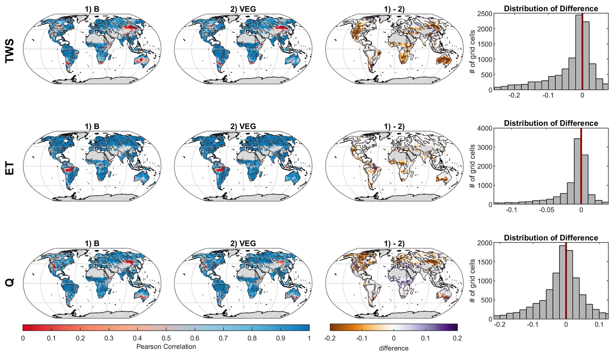
Figure 4 Grid-wise Pearson's correlation coefficient for total water storage (TWS), evapotranspiration (ET), and runoff (Q) between (1) observations and B and (2) observations and VEG, as well as differences between (1) and (2) (brown colour, i.e. negative values, indicates higher correlations for VEG, while purple colour, i.e. positive values, indicates better correlation values for B).

For TWS, the amplitude at the global scale is well captured yet with a phase difference of ∼1 month in both model variants, where both model variants show an earlier timing of peak storage (Fig. 3). The phase shift is also apparent in the temperate and cold regions, while the seasonal dynamics in sub-humid and humid regions is captured well, yet with an underestimation of the amplitude. Though differences are small, VEG obtains higher correlation, except for the semi-arid region. At local scale, correlation with GRACE TWS is lowest in rather semi-arid grid cells (Fig. 4), where TWS variation is low. However, including spatial patterns of vegetation improves TWS mainly in these (semi-)arid regions.

Regarding ET, both experiments reproduce seasonal dynamics in all regions quite well yet tend to underestimate ET in the semi-arid, sub-humid, and humid regions, especially in months with low ET (Fig. 3). At grid scale (Fig. 4), correlation of ET is very high, except for tropical regions due to low seasonality. Compared to B, VEG improves correlation here, as well as in some (semi-)arid regions such as the Sahel zone and the Western United States.

In contrast to ET, performance for Q is generally the best in regions with poorer model performance in terms of ET (semi-arid, sub-humid and humid regions) (Fig. 3), suggesting a trade-off between the two different observation data streams, i.e. the inability of matching both observed fluxes simultaneously. Nonetheless, including varying vegetation characteristics improves peak runoff in all regions and reduces the underestimation of Q especially in the cold region. While the improvement of Q simulations in northern latitudes gets even more obvious at grid scale, B shows higher correlation with observations in Africa and the Mediterranean (Fig. 4).

3.2 Importance of varying vegetation properties to TWS variability

In this section, we present the influences of vegetation on TWS partitioning into snow (wSnow), plant-accessible soil moisture (wSoil), not directly plant-accessible deep soil water (wDeep), and non-plant-accessible slow water storages (wSlow) at different spatial and temporal scales. We first focus on mean seasonal dynamics and continue with the contribution of each component to inter-annual TWS variability at local grid-cell and regional scales, respectively, before presenting the analysis at the global scale.

3.2.1 Local and regional scale

Figure 5 shows the contribution of individual water storages to mean seasonal TWS variations at local grid scale. For both B and VEG, wSnow has the highest impact in northern latitudes and high altitudes where snowfall occurs regularly. Locally, the contribution of liquid water increases gradually with decreasing latitude and, finally, causes all TWS variations south of ∼45^∘ N. Within the liquid water storages, B attributes nearly all variations to directly plant-accessible soil moisture wSoil, with an average of 76 % over all grid cells. While showing a similar pattern of increasing contribution towards lower latitudes, the VEG experiment only has an average of 17 % contribution from wSoil. Instead, most variations (40 %) are due to variability in the deeper soil storage, wDeep. In addition, the average impact of slow water storages wSlow (20 %) is comparable to that of wSnow (22 %) in VEG, though it is spatially much more limited to tropical regions, such as the Amazon basin.

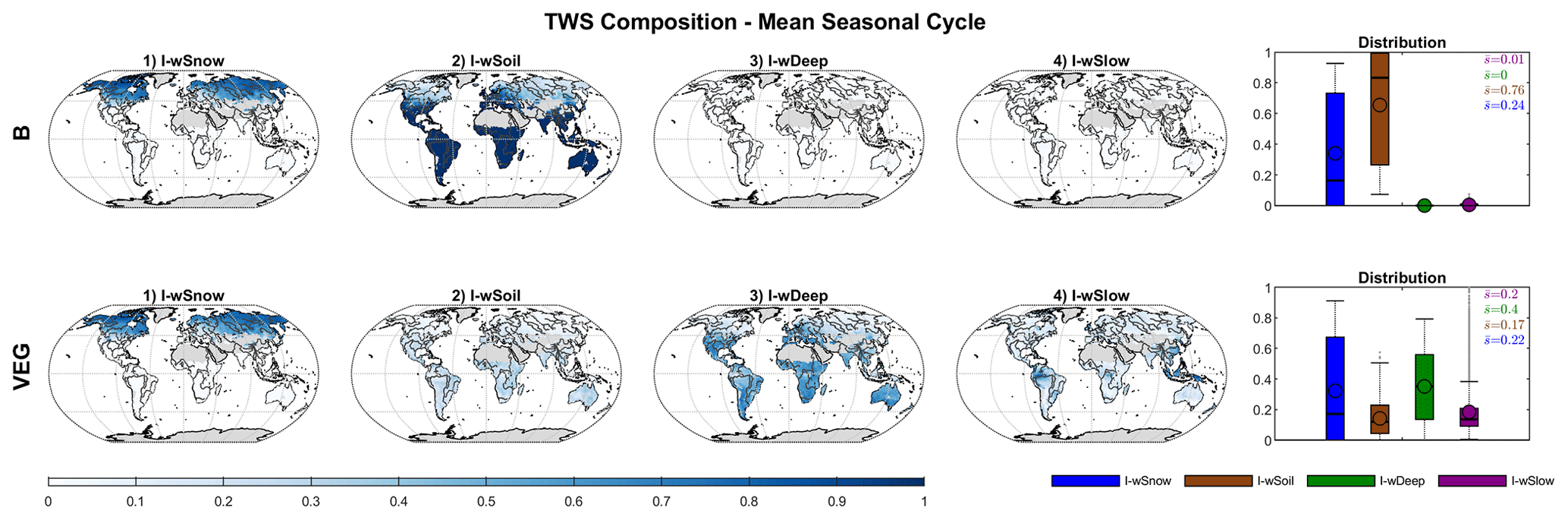
Figure 5 Global distribution of the impact index I for the contribution of simulated snow (wSnow), soil (wSoil), deep water storage (wDeep), and delayed water storage (wSlow) to the mean seasonal cycle of total water storage, for B and VEG.

Mean seasonal dynamics averaged globally and for different regions are shown in Fig. 6. As indicated by the grid-scale results, wSnow dominates TWS variations in the northern cold region (73 % in B, resp. 69 % in VEG) and plays a considerable role in the temperate region (28 % resp. 26 %). For the other regions, B attributes nearly all remaining variability to wSoil, while in VEG wDeep has the highest impact index (59 % in semi-arid, 50 % in sub-humid, and 43 % in humid).

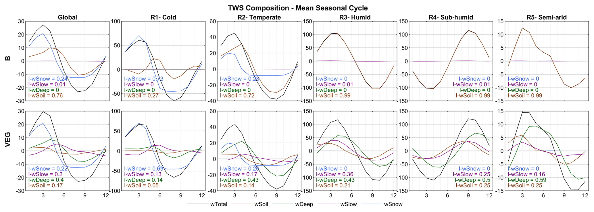
Figure 6 Global and regional average mean seasonal cycles of simulated total water storage and its components for B and VEG, including the regional impact index I for each storage.

At the inter-annual scales, the impact of wSnow decreases to 10 % (B) and 12 % (VEG) locally (Fig. 7). For most of the grid cells, all inter-annual TWS variations are caused by wSoil in B. In VEG, however, the deeper soil layer wDeep is again the most important storage, with an average impact index of 53 % for all grid cells. The contribution of wSoil and wSlow remains more or less the same as that for seasonal TWS variations.

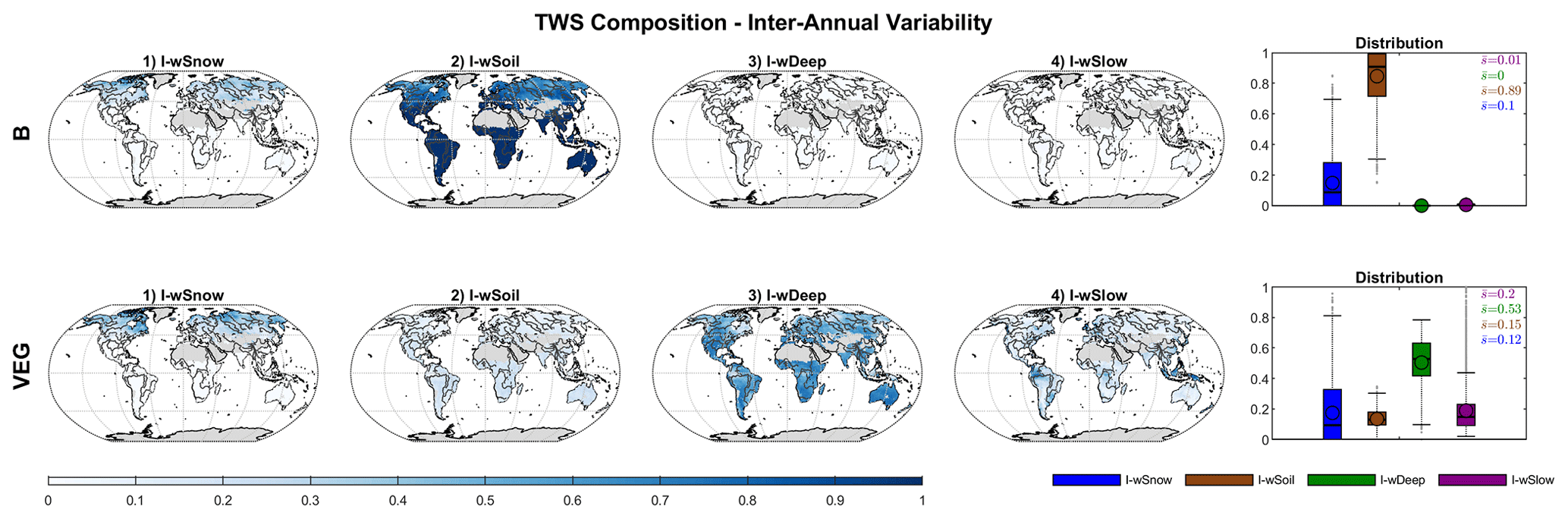
Figure 7 Global distribution of the impact index I for the contribution of simulated snow (wSnow), soil (wSoil), deep water storage (wDeep), and delayed water storage (wSlow) to the inter-annual variability of total water storage, for B and VEG.

Average contributions for different regions and globally (Sect. S4 in the Supplement) show again that, in B, nearly all inter-annual TWS variability is caused by wSoil (87 %–99 %). Only in the cold region does the impact of wSoil decrease to 69 % in favour of wSnow (31 %). Similar to the local scale, in VEG, wDeep explains >50 % of TWS variability in most regions. Only in the cold region is the contribution of wDeep similar to wSnow (39 % vs. 38 %). The contribution of wSoil ranges from 9 % (cold) to 19 % (semi-arid), while the impact of wSlow is between 16 %–18 % in most regions and increases in sub-humid (24 %) and humid (34 %) regions.

3.2.2 Global scale

Finally, Fig. 8 contrasts the impact of water storage components to the total storage, in B and VEG, at the global scale. As with the local and regional scales, including varying vegetation characteristics differentiates the composition of global TWS variations drastically. In both experiments, wSnow clearly dominates the spatially aggregated mean seasonal cycle with an impact index of 71 % (B) and 61 % (VEG). These contributions are considerably higher than the average local impact index over all grid cells (B 24 %, VEG 22 %; Fig. 5). As already seen at local scale, liquid water storages dominate the inter-annual TWS variability, whereby B and VEG differ in the attribution to different components of the liquid water storage. In B, all variations other than wSnow originate from wSoil, but wDeep dominates in VEG. Especially at inter-annual scales, wDeep accounts for half of all TWS variations. In contrast to B, in VEG, wSoil only has a minor impact of 7 % at seasonal and 13 % at inter-annual scale. Instead, wSlow has a moderate contribution of 11 % (mean seasonal) and 17 % (inter-annual). In contrast to the mean seasonal dynamics in which the dominating storages are different at local and global scales, the inter-annual dynamics are consistent across scales, with the same storage component dominating at both local and global scale (Figs. 5, 7, and 8).

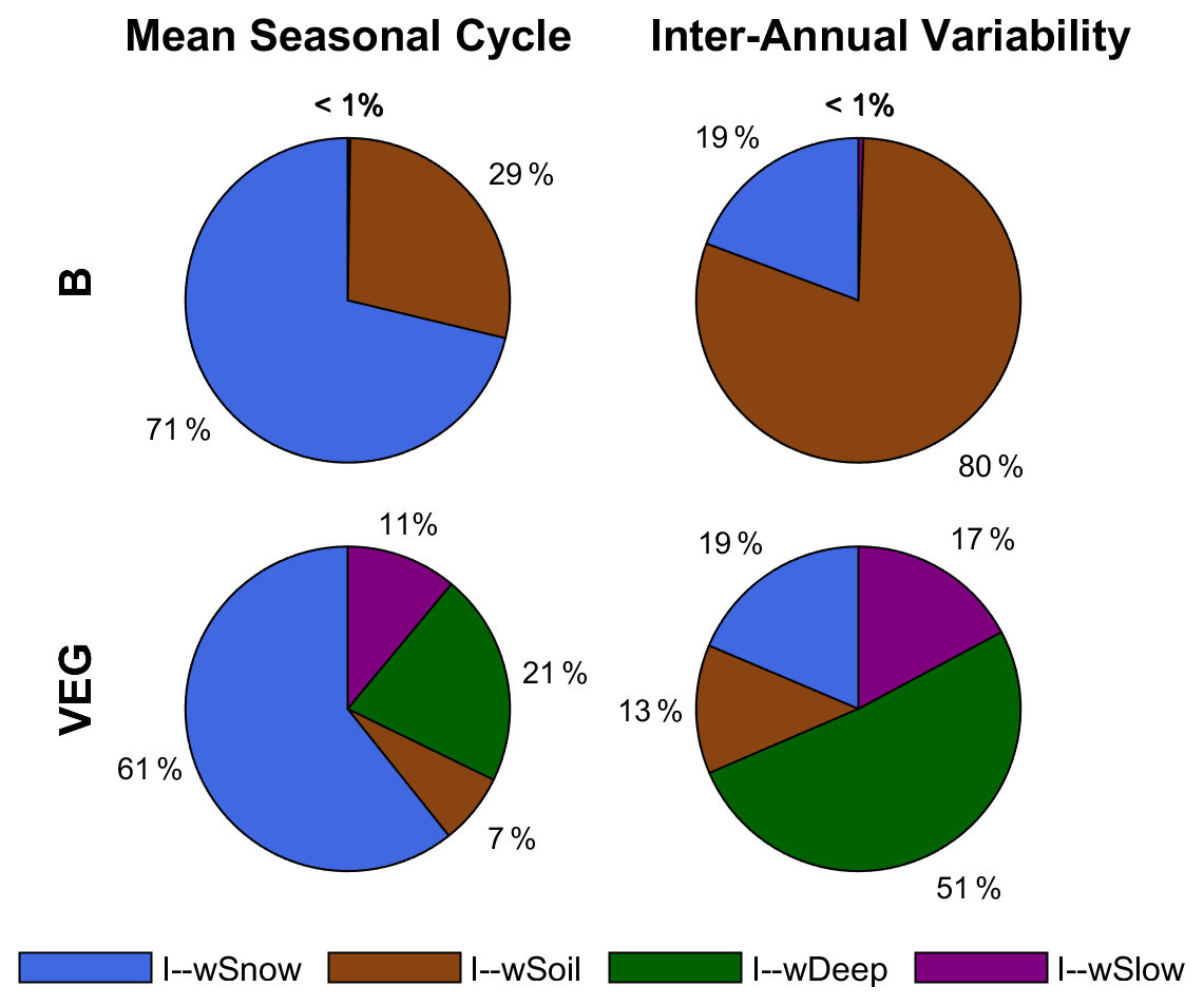
Figure 8 Impact index I for the contribution of simulated snow (wSnow), soil (wSoil), deep water storage (wDeep), and delayed water storage (wSlow) to the global average mean seasonal cycle and inter-annual variability of total water storage, for B and VEG.

4 Discussion

In order to address the two main research questions of this study, the following section discusses the above-shown differences between B and VEG, first regarding model performance and finally regarding the modelled partitioning of TWS.

4.1 Model performance

Both experiments show good performance against the observational constraints, and the differences between B and VEG are relatively small at the global scale. However, there are systematic improvements for VEG at the regional and local scale, and calibrated parameter values for VEG are more realistic and better constrained. This suggests a more realistic representation of fluxes and states in VEG overall. Remaining discrepancies compared to observations can be associated with shortcomings and uncertainties in the observational data as well as to the processes that are not represented in the rather simple model structure.

The differences in the seasonal phase of global TWS in both model experiments mainly originate from the temperate and cold regions, and such model simulation differences have been reported previously (Döll et al., 2014; Schellekens et al., 2017; Trautmann et al., 2018). One of the potential reasons is the temporary storage of meltwater during spring in rivers and other surface water bodies, which occurs contiguously over large areas in mid-latitudes to high latitudes (Döll et al., 2014; Schellekens et al., 2017; Schmidt et al., 2008; Kim et al., 2009) and which delays the storage decay. In this context, lateral water transport may also additionally affect the TWS variations in downstream grid cells. Yet, such processes and conditions are neither represented in B nor VEG.

Weaker performance of TWS in (semi-) arid regions is likely mainly due to low observed TWS variations and a low signal-to-noise ratio (Scanlon et al., 2016). Hence, less weight is also given to those grid cells in the cost component during calibration due to their small variations. In addition, alteration by human activities like groundwater withdrawal, dams, and irrigation to overcome the natural water shortage in such regions as Northeast China and the American (Mid)West can be regionally large in relative terms. While we aimed to exclude grid cells with large human impact a priori, we cannot completely exclude the influence of the aforementioned anthropogenic processes that are not explicitly represented in our model experiments. It should, however, be noted that the observational EVI data used in the VEG experiment do have an imprint of, for example, irrigated agriculture, as the measured surface reflectance includes the higher vegetation activity due to irrigation. The better representation of ET in semi-arid regions due to the EVI constraint contributes to the improved simulation of TWS variations in the VEG experiment.

While overall ET performance is good, tropical regions show low correlation. These areas are associated with higher uncertainties in the FLUXCOM ET estimates (Jung et al., 2019) due to underlying data uncertainties of the eddy covariance observations. Those uncertainties are related to poor station coverage and energy balance closure gap but also to issues of the satellite data inputs caused by cloud coverage. Nonetheless, including varying vegetation characteristics data improves simulated ET here, suggesting a better representation of the characteristic highly active vegetation compared to other regions and to global averages. In addition, VEG improves ET mainly in water supply-limited regions for the reasons already presented above for improved TWS performance in (semi-) arid regions.

The trade-off between the performances, in particular in terms of the bias of Q and ET, suggests larger uncertainties in one of the data streams for these regions, inconsistencies between the ET and Q constraints from independent sources, and/or model structure deficits. A small tendency to a negative water balance in the consistency checks of the observational data for these regions (Sect. S10) implies either underestimation of the precipitation forcing or overestimation of FLUXCOM ET or GRUN Q. Global precipitation datasets tend to underestimate precipitation (Trenberth et al., 2007; Contractor et al., 2020) due to limitations of the satellite retrieval, gauge measurements, and, if combined, the combination method (Fekete et al., 2004). Validation of the GPCD 1DD data used in this study showed an underestimation of precipitation in complex terrain and regionally during spring and autumn, while precipitation in wintertime tends to be overestimated (Huffman et al., 2000). While we accounted for the latter by reducing snowfall (via a scaling parameter that was calibrated in Trautmann et al., 2018), we do not consider potential underestimation in the rainfall forcing. Therefore, precipitation forcing may not provide sufficient water input for ET and Q in the model to achieve the magnitudes given by the observation-based products. Lastly, some deterioration of performance of Q in VEG may originate from deficiencies in the GRUN product itself, which was generated with climatic drivers only, disregarding information on spatio-temporal variations in vegetation (Ghiggi et al., 2019).

The improvement of Q in northern latitudes is associated with the activation of the slow and delayed storage in the VEG experiment, with spatial varying parameterization of soil water storage capacity. The relatively low storage capacity in these regions facilitates faster saturation excess runoff. In addition, the slow storage better represents the runoff delay in surface water and rivers in these regions that results in improvements of low flow during winter as well as the increase of runoff during spring (Fig. 3). Such delayed runoff also improves the simulation of peak runoff in the sub-humid and humid regions.

The remaining deficiencies in model performance, especially in the cold region, indicate missing processes in the simple model structure. Such processes include freeze–thaw dynamics and permafrost (Yu et al., 2020) as well as ice jam in river channels that would increase surface water storage and allow for high spring flood (Kim et al., 2009). In addition, snow parameters have been calibrated against remote-sensing-based GlobSnow snow water equivalent, that is known to saturate for deep snow conditions (Takala et al., 2011) (see Trautmann et al., 2018). Although the calibration process considered this shortcoming, an underestimation of modelled snow accumulation is possible – leading to an underestimation of peak snowpack in winter that would result in an underestimation of runoff due to lower snowmelt in spring.

While the VEG experiment presented here considers all three aspects of vegetation influences on hydrological processes explicitly (see Sect. 2.2.1), we also run experiments that include these aspects separately in the model calibration (not shown). These analyses found that the largest improvement was obtained when including soil water storage capacity as a function of rooting depth and storage capacity data and a rather low impact when considering the runoff/infiltration partitioning as a function of the vegetation fraction. This highlights the central role of soil water storages and the importance of adequately describing soil moisture pattern and dynamics in hydrological models.

4.2 Contribution to TWS variability

Albeit their global coverage, the above-presented results agree with the previous regional study that focused on northern mid-latitudes to high latitudes (Trautmann et al., 2018). Similarly, both model experiments show a dominating role of snow accumulation and depletion on global seasonal TWS variability, whereas liquid water storages determine inter-annual TWS variations. At the same time, the contribution of individual storages to TWS variations differs at the local grid scale compared to when they are averaged over a region or globally. The stronger contribution of snow on spatially aggregated signals can be explained by the spatial coherence of snow accumulation over larger areas. Liquid water storages, on the other hand, are more spatially heterogeneous, with increasing and decreasing dynamics across regions that cancel out and compensate for each other when spatially aggregated (Trautmann et al., 2018; Jung et al., 2017). In contrast to the mean seasonal dynamics, the inter-annual impact indices of the storage components at the global scale are similar to the average local impact indices (Figs. 7 and 8). This suggests that at inter-annual timescales, there is no spatially coherent pattern of one single storage component that leads to higher accumulated impact indices than the local averages. However, while both experiments agree in the general pattern of the impact of snow versus liquid water storages, they systematically differ in the allocation of water among liquid storage compartments. In B, all variations other than wSnow originate from directly plant-accessible soil moisture, whereas, in VEG, the deeper soil storage wDeep becomes the most important. Therefore, including observation-based information on vegetation changes the attribution of TWS variations drastically, while the variations of total TWS themselves do not change significantly.

Differences in the composition of TWS variability between B and VEG are effectively reflected in the differences of calibrated parameters. In B, the directly plant-accessible soil water storage is larger, due to a higher effective wSoil_max(2), while delayed water storages are “turned off” because of increased drainage (d_Deep, d_Slow), reducing the variations in wDeep and wSlow. Although VEG has been calibrated in the same way as the same observational constraints, calibrated model parameters differ as the data on vegetation characteristics included provide complementary information on spatial and temporal patterns. Therefore, the resulting calibrated parameters can be assumed to be more realistic. For example, they enable (delayed) longer term water storage as well as capillary rise from the deeper soil water storage when the directly plant-accessible storage dries out. Due to this process, TWS variations are mainly controlled by wDeep in VEG.

In detail, the increased importance of the indirect plant-accessible storage wDeep in VEG can be related to the limited maximum soil water capacity wSoil_max(2) that is constrained by rooting depth–soil water capacity data and to a higher k_Transp parameter. The smaller wSoil storage increases percolation to wDeep, but the water is still available when needed due to the capillary rise from wDeep to wSoil.

Removing capillary flux from wDeep to wSoil in fact increases the contribution of wSoil to seasonal variability, while the impact of wDeep remains high on inter-annual scales (Sect. S7 in the Supplement). While the contribution of capillary rise to total ET is <20 % for most grid cells, it becomes more important in arid-to-wet transition regions, for example, sub-Saharan Sahel, Savannas, northern Australia, and the Indian subcontinent (Fig. 9). These are regions with high precipitation seasonality, where vegetation often grows deep roots to access deep unsaturated zone storage and groundwater during the dry season. The spatial patterns of ET supported by capillary rise agree with the findings of Koirala et al. (2014), who applied the physically based model MATSIRO to investigate the effect of capillary flux on hydrological variables. The spatial patterns are also in line with the predicted probability of deep rooting by Schenk and Jackson (2005) and are supported by Tian et al. (2019), who found that vegetation remains active long into the dry season in Africa, suggesting that soil–deep soil–groundwater interaction plays a considerable role. Therefore, the spatial pattern of the interactions of wDeep with wSoil in VEG seems reasonable, and our results indicate that capillary rise appears to be a process of large-scale relevance.

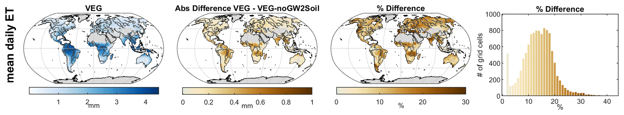
Figure 9 Total evapotranspiration (ET) of VEG with capillary flux from the deep soil water storage (left) and difference compared to a model version without capillary flux in millimetres (right map) and as a percentage difference (right).

While defined as the “fraction of soil water available for transpiration”, k_Transp is an effective decay parameter for the depletion of wSoil via transpiration processes under water-limited conditions. Plausible values derived from eddy covariance observations of ET are in the order of 10⁻³–10⁻¹ (Teuling et al., 2006), similar in magnitude to delay coefficients for baseflow. By calibrating a model against GRACE TWS, it is difficult to decide whether water leaves the system slowly via ET or by Q, especially during drydown periods. In B, k_Transp is much smaller than in VEG and more consistent with expected magnitudes, yet other slow depleting storages are effectively “turned off”. In contrast, VEG with additional vegetation data simulates an important slow storage that contributes to Q and also to soil moisture via capillary rise and has a rather high calibrated k_Transp. To better understand the implications of parameterizing supply-limited ET decay in the model, we conducted another experiment where we fixed k_Transp in VEG to 0.05 (about the median value of empirically derived k_Transp from Teuling et al., 2006) and optimized all other parameters again. This caused most TWS variations to originate from wSoil but with less improvement in model performance compared to B (Sect. S8 in the Supplement). Therefore, TWS decomposition is very sensitive to parameters controlling ET under water-limited conditions. However, VEG and VEG with fixed k_Transp qualitatively agree in the importance of the slow water storage in humid regions, which was also shown by Getirana et al. (2017). Overall, our results imply that the representation of ET under water-limited conditions in the models plays a decisive role in the simulated partitioning of TWS in soil moisture and slow water pools.

The large impact of the role of vegetation and of transpiration water supply within the model is also supported by a complementary experiment in which vegetation parameters were discretized for plant functional type classes and calibrated with the same multi-criteria approach (Sect. S9).

As with the presented model variants, TWS composition simulated with existing large-scale hydrological models differs widely (Scanlon et al., 2018; Schellekens et al., 2017; Zhang et al., 2017). For example, PCR-GLOBWB and W3RA attribute seasonal TWS variations in the tropics to groundwater, while other models suggest they are mainly caused by soil moisture. These results are largely dependent on model structure and parametrization, which is potentially a challenge when models are used to decompose the integrated GRACE TWS signal and when implications of different processes and interactions are drawn. For example, Humphrey et al. (2018) analysed how the CO₂ growth rate, a proxy for the land carbon balance fluctuations, is affected by inter-annual variations in GRACE TWS, assuming that these represent fluctuations in plant-accessible water that influence the carbon uptake of land ecosystems. In contrast, our study, along with previous reports, shows that a significant proportion of the GRACE TWS signal in the tropics is not directly plant-accessible soil moisture but deeper soil water and slow storage components. The latter comprises surface water storage, whose importance for TWS variations in tropical regions has been shown by several studies (e.g. Güntner et al., 2007; Getirana et al., 2017).

Although VEG can be considered more reliable because of more realistic parameter values and better model performance, the current study still has some shortcomings. Despite using a multi-criteria calibration, individual component fluxes and states may not necessarily be well constrained. To further improve and solidify conclusions, especially on TWS partitioning, more constraints, such as deep soil moisture estimates or high-quality observations of surface water, are needed. Furthermore, spatial constraints for defining the depletion of water storages via ET and Q – either with spatial information on the delay parameters (k_Transp for ET, d_Slow for Q) or on their sub-fluxes (transpiration or evaporation, baseflow or direct runoff) – would be beneficial. In this context, runoff characteristics as the baseflow index or the baseflow recession coefficient provided by Beck et al. (2015) are potentially useful to define the spatial pattern of the slow runoff component. In addition, a GRACE product with daily resolution (Eicker et al., 2020) could enable better decomposition and differentiation of fast and slow storages whose short-term imprints are lumped in the monthly TWS signal.

5 Conclusions

In this study, we investigated the effect of varying vegetation characteristics on global hydrological simulations and in particular on the partitioning of TWS variations among snow, plant-accessible soil moisture, a deep soil water storage, and a slowly varying water pool that represents groundwater, surface and near-surface water storage. To do so, we included observation-based continuous vegetation information to parameterize the hydrological processes of evapotranspiration, soil water storage, and runoff generation in a large-scale hydrological model. With the parsimonious model that was constrained against multiple observations, we highlight the value of observation-based datasets in constraining model parameters of global hydrological models while maintaining simple model formulations to evaluate the influences of vegetation in the global hydrological cycle.  First, we find that using a multi-criteria calibration approach allows for different model variants to perform relatively well despite major differences in model parameterization among them. In fact, even without accounting for dynamics and patterns of vegetation explicitly, the model performance can be interpreted as reasonable and more so at the global scale. However, including the spatial pattern of vegetation further improved the model performance. For example, large improvements were found in supply-limited regions, i.e. (semi-) arid regions (TWS and ET) and in tropical regions (ET), and Q simulations both globally and regionally in the Northern Hemisphere. Undoubtedly, spatio-temporal variations of vegetation characteristics are relevant for regional and global hydrological simulations.

Interestingly, we find that the calibrated parameter values are also more reasonable when the model is fed with the vegetation information. In particular, parameter interactions and equifinality were reduced even though the same observational constraints were used for calibration.

Lastly, we show how the representation of vegetation can modulate surface and subsurface hydrological process representation in the model, changing the spatial–temporal dynamics of individual storage components while maintaining the same overall response of total hydrological fluxes and storage variations. With or without accounting for varying vegetation characteristics explicitly, seasonal storage variations are dominated by snow at the global scale. However, including varying vegetation characteristics drastically changes the attribution of TWS variations among soil moisture, deep soil water, and slow water storages. Without varying vegetation parameters, the soil moisture effectively controls most of the TWS variation, but with varying vegetation characteristics, the role of deeper and delayed water storage becomes prominent. In particular, the representation of water-limited ET by the interplay of its sensitivity to soil moisture, maximum plant-accessible water storage capacity, and interactions with deep soil moisture or groundwater seem to play a decisive role in TWS partitioning in the simulations.

In summary, this study highlights the value of including varying vegetation characteristics to further constrain model parameters with a parsimonious model structure. The findings further suggest an important role of groundwater–soil moisture–vegetation interactions in TWS variations. Since the representation of vegetation-related processes in global hydrological models seems to be a key factor for controlling TWS partitioning, we emphasizes the need for further studies and improvements of global water cycle models with respect to the role of vegetation by utilizing observational constraints on ecohydrological functioning in multi-criteria model calibration exercises.