Accretion, retreat and transgression of coastal wetlands experiencing sea-level rise

The vulnerability of coastal wetlands to future sea-level rise (SLR) has been extensively studied in recent years, and models of coastal wetland evolution have been developed to assess and quantify the expected impacts. Coastal wetlands respond to SLR by vertical accretion and landward migration. Wetlands accrete due to their capacity to trap sediments and to incorporate dead leaves, branches, stems and roots into the soil, and they migrate driven by the preferred inundation conditions in terms of salinity and oxygen availability. Accretion and migration strongly interact, and they both depend on water flow and sediment distribution within the wetland, so wetlands under the same external flow and sediment forcing but with different configurations will respond differently to SLR. Analyses of wetland response to SLR that do not incorporate realistic consideration of flow and sediment distribution, like the bathtub approach, are likely to result in poor estimates of wetland resilience. Here, we investigate how accretion and migration processes affect wetland response to SLR using a computational framework that includes all relevant hydrodynamic and sediment transport mechanisms that affect vegetation and landscape dynamics, and it is efficient enough computationally to allow the simulation of long time periods. Our framework incorporates two vegetation species, mangrove and saltmarsh, and accounts for the effects of natural and manmade features like inner channels, embankments and flow constrictions due to culverts. We apply our model to simplified domains that represent four different settings found in coastal wetlands, including a case of a tidal flat free from obstructions or drainage features and three other cases incorporating an inner channel, an embankment with a culvert, and a combination of inner channel, embankment and culvert. We use conditions typical of south-eastern Australia in terms of vegetation, tidal range and sediment load, but we also analyse situations with 3 times the sediment load to assess the potential of biophysical feedbacks to produce increased accretion rates. We find that all wetland settings are unable to cope with SLR and disappear by the end of the century, even for the case of increased sediment load. Wetlands with good drainage that improves tidal flushing are more resilient than wetlands with obstacles that result in tidal attenuation and can delay wetland submergence by 20 years. Results from a bathtub model reveal systematic overprediction of wetland resilience to SLR: by the end of the century, half of the wetland survives with a typical sediment load, while the entire wetland survives with increased sediment load.

1 Introduction

The vulnerability of coastal wetlands to future sea-level rise (SLR) has been extensively studied in recent years, and models of coastal wetland evolution have been developed to assess and quantify the expected impacts (Alizad et al., 2016b; Belliard et al., 2016; Clough et al., 2016; D'Alpaos et al., 2011; Fagherazzi et al., 2012; Kirwan and Megonigal, 2013; Krauss et al., 2010; Lovelock et al., 2015b; Mogensen and Rogers, 2018; Rodriguez et al., 2017; Rogers et al., 2012; Schuerch et al., 2018). Predictions vary widely, which is not surprising given the complexity of the processes involved and the practical challenges associated with representing interactions at a variety of spatial and temporal scales. Coastal wetlands respond to SLR by vertical accretion and landward migration. Vertical accretion occurs due to the capacity of wetland vegetation to trap sediments and to incorporate dead leaves, branches, stems and roots into the soil, building up their vertical elevation and counteracting submergence due to SLR. Landward migration is driven by the preferred inundation conditions of wetland vegetation, which is continuously moving up the wetland slope due to SLR. These two main processes interact, but they also integrate a number of biophysical exchanges that occur on smaller scales. Accretion is a function of many other variables like the tidal regime, sediment availability and type of vegetation (Fagherazzi et al., 2012; Lovelock et al., 2015a). Vegetation preference is dictated by salinity, oxygen availability and the presence of phytotoxins in the soil (Bilskie et al., 2016; Crase et al., 2013).

Studies show that different modelling approaches used to address the interaction between these variables may lead to divergent results (Alizad et al., 2016a; Rogers et al., 2012). For the sake of simplicity, some previous studies have adopted an approach where water levels throughout the wetland remain the same as those observed at the inlet, i.e. the bathtub approach (D'Alpaos et al., 2011; Kirwan and Guntenspergen, 2010; Kirwan et al., 2010, 2016a; Lovelock et al., 2015b). Most of these bathtub model results show that vegetation in coastal areas can produce accretion rates similar to sea-level rise predictions, therefore maintaining their elevation in the tidal prism, except when tidal range and sediment supply are very low. However, the projections of coastal wetland resilience under high rates of SLR appear to be at odds with paleo-environmental reconstructions of wetland responses to rising seas during the early Holocene (Horton et al., 2018; Saintilan et al., 2020). One explanation for this discrepancy is that models fail to reproduce the flow attenuation caused by the friction induced by substrate cover and specific wetland features like inner channels, embankments and flow constrictions (Hunt et al., 2015) and its effects on sediment availability, which may result in overestimation of wetland accretion rates (Rodriguez et al., 2017). Bathtub models do not provide information on flow discharges or velocities, so they need an independent specification of sediment concentration.

On the other hand, more detailed description of hydrodynamic and sediment transport mechanisms can be incorporated into the computations of wetland dynamics using conventional two- or three-dimensional flow and sediment transport models (Ganju et al., 2015; Lalimi et al., 2020; Temmerman et al., 2005). A detailed description of flow and sediment transport processes can potentially result in a better estimation of wetland dynamics including accretion and migration processes, but implementation can be seriously limited by computational cost and data availability (Beudin et al., 2017).

Here, we investigate how accretion and migration processes affect wetland response to SLR using a computational framework that integrates detailed hydrodynamic and sediment transport mechanisms that affect vegetation and landscape dynamics and that is efficient enough to allow the simulation of long time periods. The framework consists of a fast-performance quasi-two-dimensional hydrodynamic model (Riccardi, 2000; Rodriguez et al., 2017) that we have extensively tested in wetlands (Rodriguez et al., 2017; Saco et al., 2019; Sandi et al., 2018, 2019, 2020a, b) and a sediment advection transport model (Garcia et al., 2015) that we couple with vegetation formulations for preference to tidal conditions to obtain realistic predictions of wetland accretion and migration under SLR. Our framework incorporates two vegetation species, mangrove and saltmarsh, and accounts for the effects of manmade features like inner channels, embankments and flow constrictions due to culverts. We apply our model to simplified domains that represent distinct areas within a real wetland, in which we are able to characterise the effects of particular natural and manmade wetland features like vegetation types, culverts, embankments and channels.

Coastal wetlands are found over a broad spectrum of geomorphological settings (Woodroffe et al., 2016) and under a diverse set of anthropogenic interventions (Temmerman and Kirwan, 2015). While our results strictly apply to areas in a particular wetland in south-eastern Australia, each of our selected domains focusses on specific geomorphological characteristics that may also be present in other wetlands worldwide. We study wetland evolution on domains with no drainage network or manmade structures, which is relevant for some low-tide wetland environments where no human intervention has occurred (Leong et al., 2018; Oliver et al., 2012; Tabak et al., 2016). We simulate the dynamics of internal channels, which can provide insight into wetland studies with strong influence of natural channels (Reef et al., 2018; Silvestri et al., 2005) or manmade drainage channels (Manda et al., 2014). We carry out simulations with embankments and culverts representing flood-sheltered environments, which can resemble intentional flood attenuation works for coastal protection (Van Loon-Steensma et al., 2015) or unintentional flood attenuation as a result of roads, tracks, pipes and other infrastructure typical of heavily human-occupied coasts (Kirwan and Megonigal, 2013; Rodriguez et al., 2017; Temmerman et al., 2003).

Also, and in order to make our results more widely relevant, we analyse the sensitivity of our predictions to the sediment load coming into the wetland by including sediment-poor and sediment-rich simulations. The incoming sediment load has been proposed as one of the main factors influencing the resilience of coastal wetlands to SLR (Lovelock et al., 2015a; Schuerch et al., 2018) and is one of the components of predictive wetland evolution models with more uncertainty, due both to our limited understanding of sediment–flow–vegetation processes and our inability to predict sediment loads in a changing future.

2 Experimental design and methods

2.1 Design of simulations

The flow in tidal wetlands can be quite complex because of the interaction of the tidal flow with natural and manmade features like vegetation, topography, channels, culverts and embankments. For that reason, results for a particular wetland may have limited applicability to another wetland with different features. In this contribution, we analyse some of the most common features of wetlands in isolation in order to gain a better understanding of the contribution of each feature to the overall wetland response and how it influences the response to sea-level rise. For that purpose, we study the response of wetlands with limited complexity using a state-of-the-art ecogeomorphological model on four hypothetical tidal flats that characterise specific areas of a typical south-eastern Australian coastal wetland that we have studied before (Fig. 1a, b) (Rodriguez et al., 2017). Simulation 1 uses a bathtub approach over a consistently sloping tidal flat initially vegetated by mangrove, saltmarsh and freshwater vegetation (Fig. 1c), in which water levels are considered uniform over the domain and no special features are taken into account. In contrast, for Simulations 2 to 5, water levels are calculated with the hydrodynamic model, which allows for the inclusion of attenuation effects from vegetation and special features. Simulation 2 considers a vegetated sloping tidal flat with no special features, Simulation 3 incorporates a drainage channel 0.4 m deep and 5 m wide to the vegetated tidal flat, Simulation 4 includes an embankment with a culvert (0.8 m wide and 0.5 m tall) in the middle of the vegetated flat, and Simulation 5 combines both a drainage channel and an embankment with a culvert (Fig. 1d). These different setups can characterise different settings found in wetlands but can also apply to different parts of a more complex wetland, as shown in Fig. 1b. In all simulations the tidal flat is 620 m long (main flow direction) and 310 m wide (cross section), divided into 10 m by 10 m grid cells, with a gentle slope of 0.001 m m⁻¹. Boundary conditions include input tides described by a sinusoidal function with 1.3 m amplitude and 12 h period and a constant sediment concentration at the wetland inlet (Fig. 1c). In each simulation we tested wetland evolution under sea-level rise from 2000 to 2100 (high-emission scenario) by considering two sediment input conditions, a low sediment supply representing current conditions and a high sediment supply. The high sediment supply condition simulations are justified due to the uncertainty of climatic conditions and the possibility of increases in intensity of storm patterns in the area, which may result in increased sediment loads in the Hunter River. Sediment loads may also increase due to changes in land use practices (Rodriguez et al., 2020).

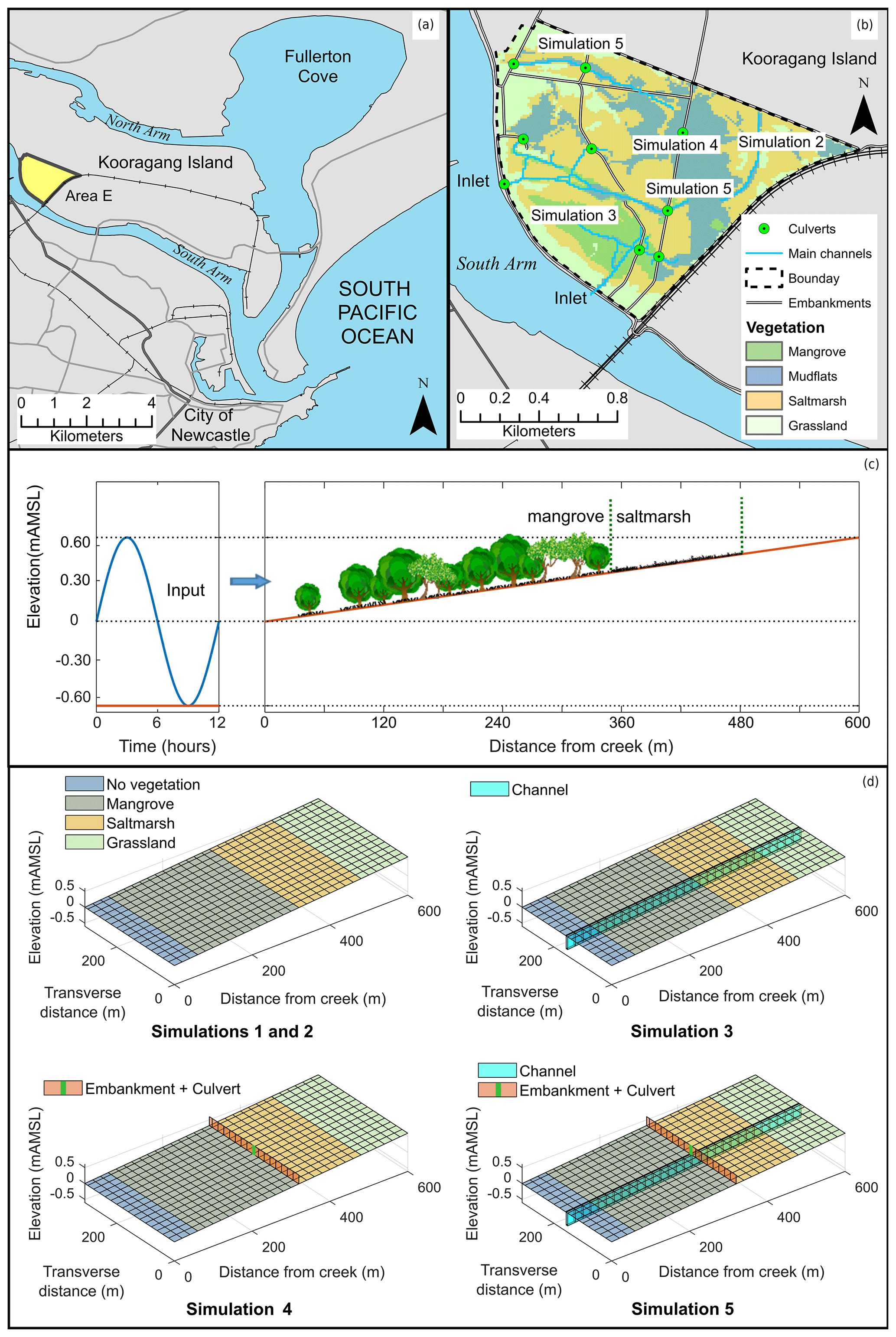
Figure 1 Field site and areas within the site characterised by the numerical simulations: (a) Area E of Kooragang wetlands, (b) areas within the wetland where the simplified simulations represent the dominant processes, (c) schematic longitudinal view of the domain setup and sinusoidal wave input (adapted from Rodriguez et al., 2017), and (d) schematic isometric view of each simulated domain and their hydraulic features. Vegetation cover is only indicative and roughly corresponds to early stages of the simulations. Elevation unit, mAMSL, stands for metres above mean sea level.

The sinusoidal tide represents conditions typical of south-eastern Australian estuaries (Rodriguez et al., 2017) and is repeated during the simulation period (100 years). However, the mean water level is gradually increased following the IPCC RCP 8.5 scenario of sea-level rise (Church et al., 2013) with an expected 0.74 m increase by year 2100 with respect to the levels in the year 2000.

We use as a basis for our simulations the ecogeomorphological model (EGM) framework developed by Rodriguez et al. (2017) but with the addition of a physically based sediment transport formulation. This EGM framework has been extensively calibrated and tested in the Hunter River estuary in Australia and, as such, vegetation functions and parameters correspond to local conditions. The framework couples multiple models to simulate interactions between overland flow hydrodynamics, vegetation establishment and growth, sediment concentration and morphodynamics of the wetland.

2.2 Hydrodynamic model

Water depth time series over the tidal flat are estimated using a finite-differences quasi-two-dimensional hydrodynamic model (Riccardi, 2000) that has been successfully applied to coastal wetlands (Rodriguez et al., 2017; Sandi et al., 2018) and floodplains (Sandi et al., 2019, 2020a, b; Saco et al., 2019). The model solves the shallow water equations using a cells scheme, in which cells are classified into tidal flat or channel categories to speed up computations. As previously explained, the domains of all simulations are 630 m long by 310 m wide, discretised into 10 m×10 m cells. For cells representing channels in Simulations 3 and 5, the width of the cell is reduced to 5 m and the elevation is lowered by 0.4 m. Boundary conditions include water elevations at the tidal creek and no flow at the lateral and landward boundaries. Because the domains are wide, the effects of lateral model boundaries are minimal.

In each time step, the model solves for water elevations at every cell using mass conservation in a two-dimensional formulation, and then it solves for discharges between cells in each direction using momentum conservation in a one-dimensional formulation. Mass conservation is solved first to compute water surface elevations:

$$\begin{array}{}\text{(1)}& {\mathrm{As}}_i{\displaystyle \frac{\mathrm{d}{z}_i}{\mathrm{d}t}}={\sum }_{k=\mathrm{1}}^j{Q}_{k,i},\end{array}$$

where As_i and z_i are surface wetted area and water surface elevation at cell i respectively and Q_k,i are the discharges between cell i and its j neighbouring cells. Using the water surface elevations, the model then computes discharges between cells using the momentum or energy equation, depending on the particular characteristics of the connection between cells. For instance, the discharge between two cells on the vegetated tidal flat is computed as

$$\begin{array}{}\text{(2)}& Q_{k,i}={\displaystyle \frac{A_{k,i}{R}_{k,i}^{\frac{\mathrm{2}}{\mathrm{3}}}}{n_{k,i}}}{\left({\displaystyle \frac{z_k-z_i}{x_k-x_i}}\right)}^{\frac{\mathrm{1}}{\mathrm{2}}},\end{array}$$

where A_k,i, R_k,i and n_k,i are respectively the cross-sectional values of area, wetted perimeter and Manning roughness computed as an average of the values at cells k and i, and x_k−x_i is the distance between cells. Based on Rodriguez et al. (2017) we adopt roughness coefficients for mangrove and saltmarsh cells of 0.50 $\mathrm{s}{\mathrm{m}}^{-\mathrm{1}/\mathrm{3}}$ and 0.15 $\mathrm{s}{\mathrm{m}}^{-\mathrm{1}/\mathrm{3}}$ respectively. For freshwater and non-vegetated cells, Manning's n is 0.12 $\mathrm{s}{\mathrm{m}}^{-\mathrm{1}/\mathrm{3}}$, while for the channel cell it is 0.035 $\mathrm{s}{\mathrm{m}}^{-\mathrm{1}/\mathrm{3}}$. For cells in the channel, the full momentum equation is used to account for dynamic and backwater effects (Riccardi, 2000). If the domain includes a culvert at cell i, then the discharge between cells k and i is computed as

$$\begin{array}{}\text{(3)}& Q_{k,i}={\displaystyle \frac{{\left(\mathrm{2}g\right)}^{\frac{\mathrm{1}}{\mathrm{2}}}{\left(z_k-z_i\right)}^{\frac{\mathrm{1}}{\mathrm{2}}}}{{\left(\frac{\mathrm{1}}{C_{\mathrm{d}}^{\mathrm{2}}{A}_i^{\mathrm{2}}}-\frac{\mathrm{1}}{A_k^{\mathrm{2}}}\right)}^{\frac{\mathrm{1}}{\mathrm{2}}}}},\end{array}$$

in which A_i and A_k are respectively the cross-sectional areas at the i and k cells and C_d is a standard discharge coefficient for the culvert at cell i adopted as 0.8. Equation (3) considered the case of the culvert flowing under the influence of gravity. For pressurised conditions, a different equation is used (Riccardi, 2000).

The model equations are solved using an implicit method and a Newton–Raphson algorithm. The time step used in the model solution is 1 s to ensure numerical stability. Further explanation about the application of this model in a similar EGM framework can be found in Sandi et al. (2018).

2.3 Vegetation model

Vegetation in coastal wetlands is driven by the tidal regime, so we use water depth time series to compute the mean depth below high tide, D, and the hydroperiod, H, on every cell as a descriptor of the tidal regime. These variables are the input for all the other models of the EGM framework. The first variable represents the average maximum water depth on spring tides. In this case we use a sinusoidal wave, so D is the maximum depth. The hydroperiod accounts for the duration of the inundation period and is computed as the proportion of time during which a minimum water depth is present during the simulation time.

The values of H and D define the suitable conditions for vegetation establishment and survival at each point in the wetland based on thresholds that have been tested for south-eastern Australian estuaries (Rodriguez et al., 2017). Thus, the observed threshold applies to Avicennia marina (grey mangrove) and to a composition of saltmarsh species Sarcocornia quinqueflora and Sporobolus virginicus. Mangrove depends primarily on hydroperiod, requires frequent inundations and establishes itself in areas where $\mathrm{10}\mathit{\%}<H<\mathrm{50}\mathit{\%}$ and D>0.2 m, where H is calculated as the fraction of time where the water depth is higher than or equal to 14 cm, the typical height of the pneumatophores. Saltmarsh tolerates prolonged inundations and can survive in areas where H<80 % but cannot endure inundation depths above its height (25 cm), so we limit D<0.25 m. We consider that, if conditions suit both mangrove and saltmarsh, mangrove will expand over saltmarsh areas (Saintilan et al., 2014). In areas not exposed to saltwater (H=0 %, D∼0 m), we assume the presence of freshwater vegetation, and if none of the above conditions applies, areas are considered to be non-vegetated.

2.4 Sediment model

The original version of the framework used in the Hunter estuary applies a linear empirical relationship between average sediment concentration in the water column and the water depth. Here, we use a more physically based equation for fine sediment transport and deposition processes coupled to the hydrodynamic simulations. The sediment model solves the quasi-two-dimensional continuity equation of suspended sediment neglecting horizontal diffusion (Garcia et al., 2015). The continuity equation for the ith cell reads as follows:

$$\begin{array}{}\text{(4)}& {\mathrm{As}}_i{\displaystyle \frac{\mathrm{d}{\left(hC\right)}_i}{\mathrm{d}t}}={\mathrm{As}}_i{\mathit{\phi }}_i+{\sum }_{k=\mathrm{1}}^j{\left(QC\right)}_{k,i},\end{array}$$

where h_i is the water depth of cell i (m); C_i is the sediment concentration (g m⁻³), φ_i is the downward vertical flux of fine sediment ($\mathrm{g}{\mathrm{m}}^{-\mathrm{2}}{\mathrm{s}}^{-\mathrm{1}}$), and C_k,i are the sediment concentrations in the j neighbouring cells. For fine-grained sediment typical of estuarine environments, the downward flux can be expressed as (Krone, 1962; Mehta and McAnally, 2008)

$$\begin{array}{}\text{(5)}& {\mathit{\phi }}_i=-w_{\mathrm{s}}\left(\mathrm{1}-{\displaystyle \frac{{\mathit{\tau }}_{\mathrm{b}i}}{{\mathit{\tau }}_{\mathrm{d}}}}\right)C_i;{\mathit{\tau }}_b<{\mathit{\tau }}_{\mathrm{d}},\end{array}$$

where w_s is the fall/settling velocity of suspended sediment particles (m s⁻¹), τ_bi is the magnitude of bed shear stress in cell i (Pa), and τ_d is the critical bed shear stress for deposition (Pa). Velocities were converted to bed shear stresses using

$$\begin{array}{}\text{(6)}& {\mathit{\tau }}_{\mathrm{b}i}=\mathit{\rho }{C}_{\mathrm{f}}{U}_i^{\mathrm{2}}.\end{array}$$

In Eq. (6) ρ is the water density and C_f is a friction coefficient set at 0.05. The parameters w_s and τ_d were varied to reproduce similar levels of accretion observed in the wetlands where the original modelling framework was applied (Rodriguez et al., 2017). The values obtained were τ_d=0.02 Pa and $w_{\mathrm{s}}=\mathrm{2}\times {\mathrm{10}}^{-\mathrm{4}}\mathrm{m}{\mathrm{s}}^{-\mathrm{1}}$, which are consistent with values reported by Larsen et al. (2009) and Temmerman et al. (2005). This model does not have an erosion term, which is not a bad simplification over vegetated surfaces that receive flows that are typically very slow.

Equation (4) is solved using the same numerical scheme than the water mass conservation (Eq. 1), providing a time series of sediment concentrations in each cell of the domain. However, as the soil elevation model (next section) works at a larger timescale and requires the annual concentration, $\overline{C}$, a weighted average is computed for each cell:

$$\begin{array}{}\text{(7)}& \overline{C}={\displaystyle \frac{{\sum }_{t=\mathrm{0}}^M\left(C_t\times h_t\right)}{{\sum }_{t=\mathrm{0}}^M{h}_t}},\end{array}$$

where t is the time in the hydrodynamic simulation with M the final step; C_t and h_t are the sediment concentration and the water depth respectively at time t.

The sediment transport equation based on mass conservation (Eq. 4) cannot be used in the case of the bathtub simulations because the bathtub model does not provide information on water discharge and velocity. For the bathtub simulations, we used the linear relation between water depth and concentration empirically developed by Rodriguez et al. (2017). Based on the measured data, the fitted equation is

$$\begin{array}{}\text{(8)}& \overline{C}=C_{max}(\mathrm{0.55}D+\mathrm{0.32}),\end{array}$$

where $\overline{C}$ is the average sediment concentration (g m⁻³), and C_max is the concentration at the wetland inlet.

This equation is much simpler and has different parameters than the sediment transport equation; however, for very simple flow conditions it should produce comparable results. We confirmed the suitability of the simple model by comparing EGM results using the bathtub approach (with the linear sediment relation) and a full hydrodynamic and sediment transport EGM over a smooth topography. Both the hydrodynamics and the resulting elevation changes of both models were very similar (see Fig. S1 in the Supplement).

2.5 Soil elevation change model

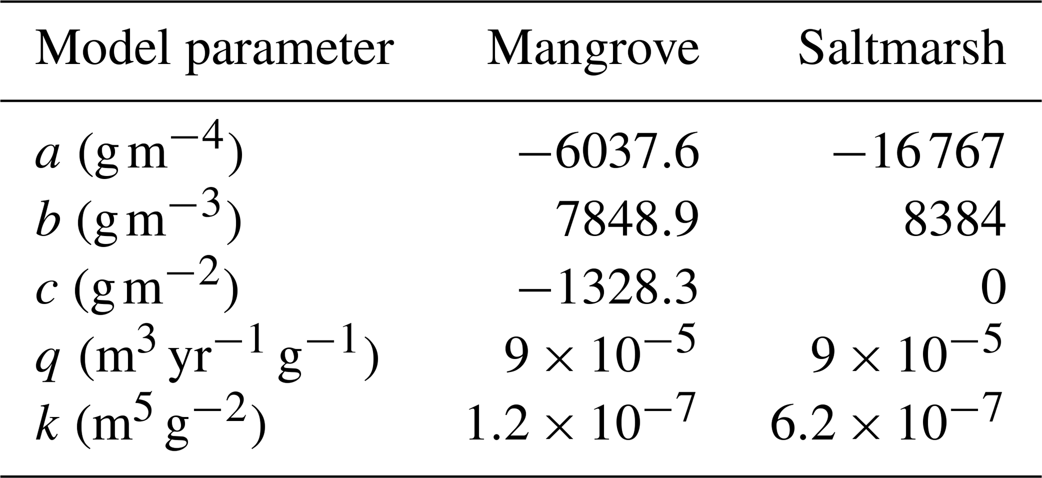
Our EGM framework adopts the model originally proposed by Morris et al. (2002) and later modified by Kirwan and Guntenspergen (2010) to estimate the increase in soil elevation due to accretion as a function of hydrodynamic and ecological conditions. We first compute the biomass production, B (g m⁻²), by using the parabolic equation

$$\begin{array}{}\text{(9)}& B=a{D}^{\mathrm{2}}+bD+c,\end{array}$$

where a, b, and c are parameters fitted to field data, for each vegetation type. Then, the surface elevation change rate, $\mathrm{d}E/\mathrm{d}t$ (m yr⁻¹), is calculated using

$$\begin{array}{}\text{(10)}& {\displaystyle \frac{\mathrm{d}E}{\mathrm{d}t}}=\overline{C}\left(q+kB\right)D,\end{array}$$

where q is a depositional parameter and k is a vegetation sediment trapping coefficient. For all five parameters of Eqs. (9) and (10) we used the values adopted in Rodriguez et al. (2017) and Sandi et al. (2018) (see Table 1) for an Australian wetland. Although the term As_iφ_i in Eq. (4) provides an amount of settled sediment that contributes to accretion, it only considers the gravitational settling of sediment and does not include many other important accretion processes associated with the presence of vegetation. The full effects of sediment and vegetation are considered in Eq. (10), which produces much larger accretion values (see Fig. S2 in the Supplement).

Table 1 Parameters of the soil surface elevation model.

The EGM simulations use a yearly time step; i.e. the computed biomass and accretion represent an average condition within this period. We choose a yearly time step as vegetation dynamics does not respond instantaneously to flow and depositional processes (Alizad et al., 2016b; Saco and Rodríguez, 2013; Schuerch et al., 2018). Our model does not account for erosion and diffusion processes and also does not take into account the redistribution of deposited sediment by waves. Because of that, the resulting accretion from Eq. (10) is noisy and varies considerably over very short distances. In order to work with a more realistic distribution of deposition over the tidal flat, we smooth the topography by applying a very simple diffusion model. The diffusion model does not change the general trends of deposition and avoids localised peaks of excessive deposition.

3 Results

3.1 Spatial patterns of accretion and vegetation

In order to show the characteristic spatial patterns of each of the typical cases analysed, we first show in Fig. 2 accumulated accretion (ΔE) and vegetation distribution in 2050 under the expected SLR scenario for each of the five numerical simulations, including the bathtub and the other four simulations that use a hydrodynamic and sediment transport (HST) model. Details on the temporal evolution of topography and vegetation for each of the simulations are provided later in the paper.

Figure 2 Accumulated accretion (top) and vegetation maps (bottom) in 2050 for low sediment input corresponding to (a) Simulation 1, (b) Simulation 2, (c) Simulation 3, (d) Simulation 4, and (e) Simulation 5.

Figure 2 shows that accumulated accretion is homogeneous in the transverse direction for the simulations without the channel (Fig. 2a, b, d), as there is no lateral flow and the changes in sedimentation occur in the longitudinal direction only. For the simulations with the central drainage channel (Fig. 2c, e) there is a marked concentration of flow and sediment accumulation close to the channel. Some of the accumulated accretion patterns of the simulations with the channel presented in Fig. 2 are remarkably similar to the results from Chen et al. (2010) on a similar geometry.

It can be seen from the figure that all simulations show a general decrease in accretion with distance to the tidal input (which can represent a tidal creek or the river), which is expected because the source of sediment is at the tidal input. However, each simulation has a characteristic elevation profile and vegetation distribution, and they are all quite different from the predictions of the bathtub model. Figure 2a shows that the bathtub simulation displays a smoother and longer transition of accumulated accretion. A slight concentration of accretion is observed at 500 m from the creek due to the initial position of high biomass saltmarsh. The bathtub case has flood and ebb flows of the same duration, since there is no flow attenuation. This keeps the hydroperiod within a range that promotes mangrove establishment over most of the wetland. Saltmarsh is limited to the upper parts of the tidal flat.

The other simulations (2 to 5) use the hydrodynamic and sediment transport (HST) models instead of the bathtub approximation. In these cases, accretion presents an exponential shape with a sharper decrease than the bathtub model, and vegetation establishment is strongly controlled by the effects of vegetation roughness, channel and culverts. In contrast to the bathtub model results, all HST simulations show mangrove dieback in lower areas, which is caused by a higher hydroperiod due to attenuated ebb flows.

Simulation 2, with the undisturbed tidal flat (Fig. 2b), shows the effect of hydraulic resistance due to the vegetation roughness only, which generates an elevation mound closer to the tidal input than the bathtub simulation. In Simulation 3 (Fig. 2c), the inner channel increases the drainage of the surrounding areas, thus reducing the hydroperiod in the vicinity of the channel and allowing mangroves to persist close to the tidal creek. The channel also enhances sediment delivery farther from the tidal input, which causes an increase in accretion around the mid-point of the flat (300 m from the tidal creek). However, this effect is concentrated near the channel and fades away as flow is directed into the tidal flat. In Simulation 4 (Fig. 2d), the flow is restricted by an embankment and a culvert, so the hydroperiods in the upper wetland are higher. This effect reduces mangrove migration and its encroachment on saltmarsh areas. In Simulation 5 with embankment and channel (Fig. 2e), the channel promotes mangrove landwards of the embankment and also the stabilisation of saltmarsh areas in the upper sections of the tidal flat as they receive more sediment (Fig. 2e).

3.2 Evolution of accumulated accretion profiles

Figure 3 shows the results of surface elevation change (ΔE) in each simulation for the years 2020, 2040, 2060 and 2100 for low sediment input conditions (corresponding to contemporary rates in the Hunter estuary), in terms of accumulated accretion profiles along the main flow direction. For the simulations with the central drainage channel (Simulations 3 and 5), we have included two profiles at different transverse locations, one close to the channel and one 150 m away in the middle of the tidal flat.

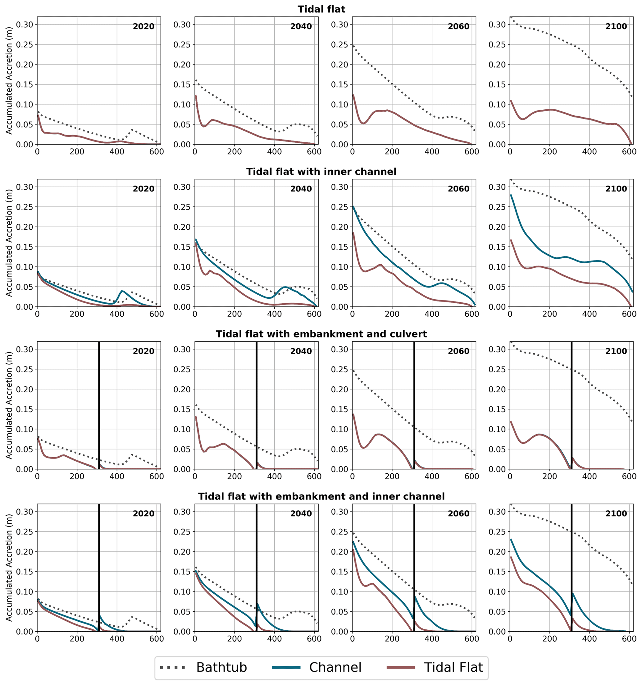
Figure 3 Longitudinal profiles of accumulated accretion (ΔE, m) for a sediment supply of 37 g m⁻³. The vertical black line represents the embankment with culvert. The “channel” profile represents the elevation gain near the central channel, while the “tidal flat” profile is situated in the middle of the tidal flat. Note: simulation starts in the year 2000.

During the first 2 decades, the vegetation type plays an important role in the longitudinal distribution of the accumulated accretion profiles. By 2020 (first column of Fig. 3) the profiles show a continuous decrease from the tidal input up to 300 to 350 m approximately, which coincides with the transition from mangrove to saltmarsh in the initial vegetation distributions (see Fig. 5 later in the paper). This occurs due to the dynamics of sediment transport (more deposition close to the tidal input) and also due to the reduction of the mangrove biomass away from the tidal creek (reductions in D; see Eq. 10). The increase in ΔE at the transition is due to the saltmarsh having a higher biomass and trapping efficiency than mangrove at that particular value of D. Landward of the transition, ΔE decreases with decreases in saltmarsh biomass. This general dynamics is disrupted by the presence of the culvert because it limits the amount of sediment reaching the upper areas of the tidal flat.

Changes in ΔE slow down after 2060 in all simulations except for the bathtub case. This is due to reductions in vegetation as most of the lower areas of the tidal flat have experienced submergence and vegetation loss. Small increases in ΔE occur in the upper areas in the cases in which the central channel promotes tidal flushing (Simulations 3 and 5), but this effect is concentrated in areas close to the channel.

None of the simulations using the HST model produces ΔE results similar to the bathtub simulations. The simulation with the central channel (Simulation 3) presents values of ΔE near the channel that are close to the results of the bathtub simulation during the first years, but over time, the results diverge. The increased ΔE values are limited to areas next to the channel, and they quickly decline as the flow is directed into the tidal flat. In general, the outcomes from the HST model show a reduction in the water levels and total accretion compared to the bathtub results. Furthermore, when the culvert is introduced in the simulation (Simulations 4 and 5), the main effect is a drastic reduction of ΔE in the upper areas of the domain.

Figure 3 results correspond to a situation with a low sediment input of 37 g m⁻³, typical of current south-eastern Australian conditions (Rodriguez et al., 2017). Similar patterns but with larger values of accumulated accretion were obtained for a higher sediment input of 111 g m⁻³ (Fig. S3 in the Supplement).

The reduction in accretion in the simulations that consider the actual features of the wetland can be better appreciated in Fig. 4, in which we compare domain-average ΔE of all simulations over time. Fig. 4 includes results for a low sediment input of 37 g m⁻³ (Fig. 4a) and for a high sediment input of 111 g m⁻³ (Fig. 4b). The figure also includes the values of mean sea level for each year to give an idea of the submergence conditions in the wetlands.

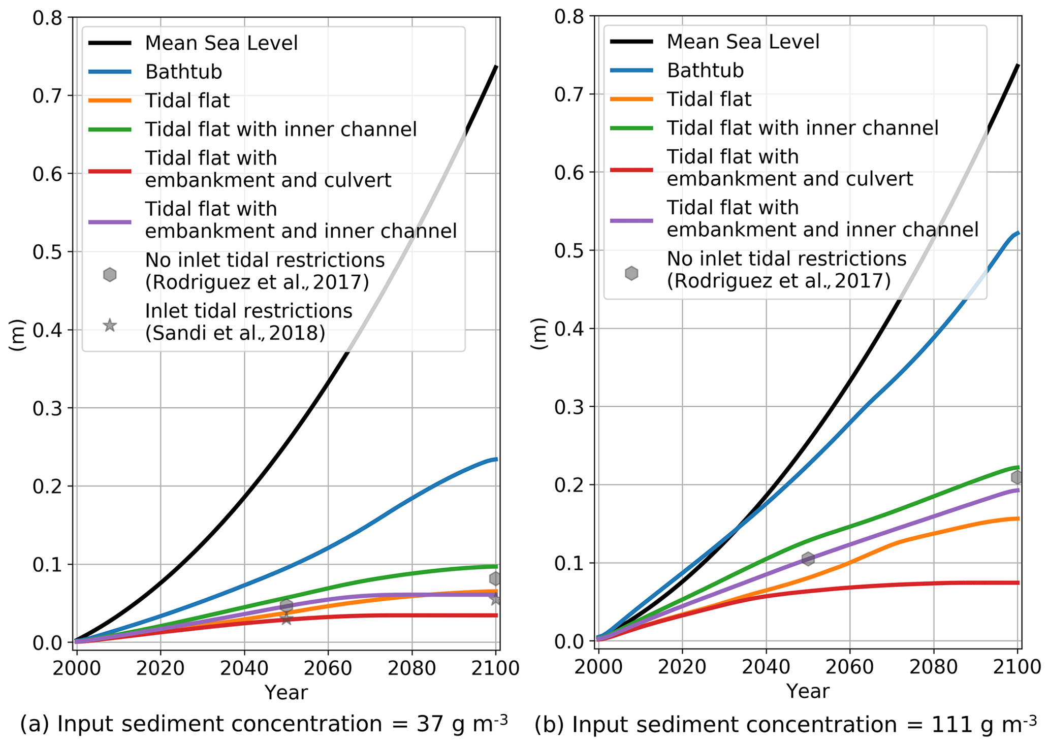
Figure 4 Sea-level rise and domain-average accumulated accretion over time for all simulations for (a) low sediment input and (b) high sediment input. Results from Rodriguez et al. (2017) and Sandi et al. (2018) corresponding to the entire Area E wetland are included for comparison.

There is a clear difference between the accretion generated in the bathtub simulation and the rest of the simulations. In our simulations, accretion is a function of sediment concentration and depth below mean high tide (D). The bathtub assumption overpredicts both inputs over the entire domain, thus generating higher accretion values. In all HST simulations, the combination of a reduction in D because of flow attenuation and the exponential decay of sediment concentration results in less accretion than in the bathtub simulation. In the case of low sediment input (Fig. 4a), by 2050 the domain-average ΔE from the bathtub is about 2 times the values of all the other simulations, increasing to more than 3 times by 2100. In the simulations with high sediment input (Fig. 4b), the accumulated accretions of bathtub simulations are 2.5 and 4 times the values of the rest of the simulations for 2050 and 2100 respectively. The simulations with the HST simulations present different levels of attenuation and accordingly different accretion levels. The lowest accretion corresponds to the highly attenuated case with embankment and culvert (Simulation 4), whereas the highest accretion occurs in the case of the central channel (Simulation 3) that experiences increased drainage and thus less attenuation. The cases of the tidal flat with no structures (Simulation 2) and of the embankment with the inner channel (Simulation 5) have intermediate levels of attenuation and accretion.

All simulations show a strong elevation deficit (i.e. the difference between the rate of sea-level rise and wetland accretion rate dE/dt), as none of the simulations predict that the tidal flat is capable of keeping pace with SLR. For the low-sediment conditions, by 2050 the elevation deficit of the bathtub simulation is 5.5 mm yr⁻¹, while the rest of the simulations predict an elevation deficit of about 7 mm yr⁻¹. Over time, the elevation deficits increase and by 2100 the bathtub predictions reach a value of 9.5 mm yr⁻¹ and the HST simulations a value of 12 mm yr⁻¹.

Increasing the sediment input concentration considerably changes the accretion capacity of the tidal flat, particularly according to the bathtub results. Bathtub simulations predict that the tidal flat is able to accrete at a rate that almost matches the changes in sea level, so the wetland survives sea-level rise. Accretions for all other simulations are moderate, with the simulations that have the central channel (Simulations 3 and 5) responding more effectively to the increased sediment and accreting more than the other simulations (Simulations 2 and 4). Compared to the low sediment conditions, elevation deficits of the bathtub predictions reduce to 3 and 5.5 mm yr⁻¹ by 2050 and 2100 respectively, while in the other simulations those values increase to about 6 and 10 mm yr⁻¹.

The structures included in the simulations have a clear effect on the average ΔE. The inner channel promotes accretion further inland, as it conveys more water and sediment to those areas away from the tidal input. Compared to the tidal flat free of structures (Simulation 2), the inclusion of the channel (Simulation 3) is responsible for an increase in wetland-accumulated accretion of about 50 %. The opposite effect is observed when the embankment with culvert is introduced, as it attenuates and reduces the water and sediment flow into the upper part of the wetland. Comparing results for the tidal flat without (Simulation 2) and with (Simulation 4) embankment and culvert, we can observe a reduction in wetland-accumulated accretion of 25 %. The introduction of a drainage channel together with the embankment and culvert (Simulation 5) represents an intermediate situation in which the increased flushing effect of the channel and the attenuating effect of the embankment and culvert partially compensate.

In Fig. 4a we have also included the average accumulated accretion for the entire wetland site (Area E in Fig. 1b) using information from Rodriguez et al. (2017) and Sandi et al. (2018). Rodriguez et al. (2017) applied a similar EGM formulation to Area E (Fig. 1c) to assess the effect of attenuation on wetland evolution under SLR considering typical (37 g m⁻³) and increased (111 g m⁻³) sediment conditions. Sandi et al. (2018) further studied the effects of tidal restrictions at the wetland inlet considering typical sediment loads. The values included in the figure correspond to average accumulated accretion over the entire wetland at 2050 and 2100 for low sediment load with and without tidal restrictions (Fig. 4a) and for high sediment load without restrictions (Fig. 4b). The figures show that the simulations without tidal restrictions result in values of accumulated accretion similar to the simulation with low attenuation (Simulations 3 and 5) for both low and high sediment loads, while predictions of accumulated accretion including tidal restrictions are closer to the simulation with high attenuation (Simulations 2 and 4).

3.3 Changes in vegetation

The interactions between sea-level rise, accretion and vegetation changes are complex because vegetation not only responds to vertical elevation changes, but also migrates inland. In order to obtain a clear picture of the vegetation changes over time, we simplified two-dimensional vegetation maps (i.e. Fig. 2) into a one-dimensional representation. The vegetation type at a given distance from the tidal input was determined by selecting the predominant (higher occurrence) vegetation in the transverse direction. Figure 5 shows snapshots of the predominant vegetation every 20 years. As already explained, in the simulations with embankment and culvert (Simulations 4 and 5), the structures are located at 310 m from the tidal input. The conditions at the beginning of the simulation (Fig. 5a) for Simulations 1, 2 and 3 show mangrove occupying approximately the lower 400 m of the tidal flat and saltmarsh the next 200 m upland. For Simulations 4 and 5 the presence of the embankment reduces hydroperiods in the upper areas, constraining mangrove to the lower 310 m. The embankment also limits the extent of inundation in the upper areas, reducing the extent of the saltmarsh to about 100 m from the embankment.

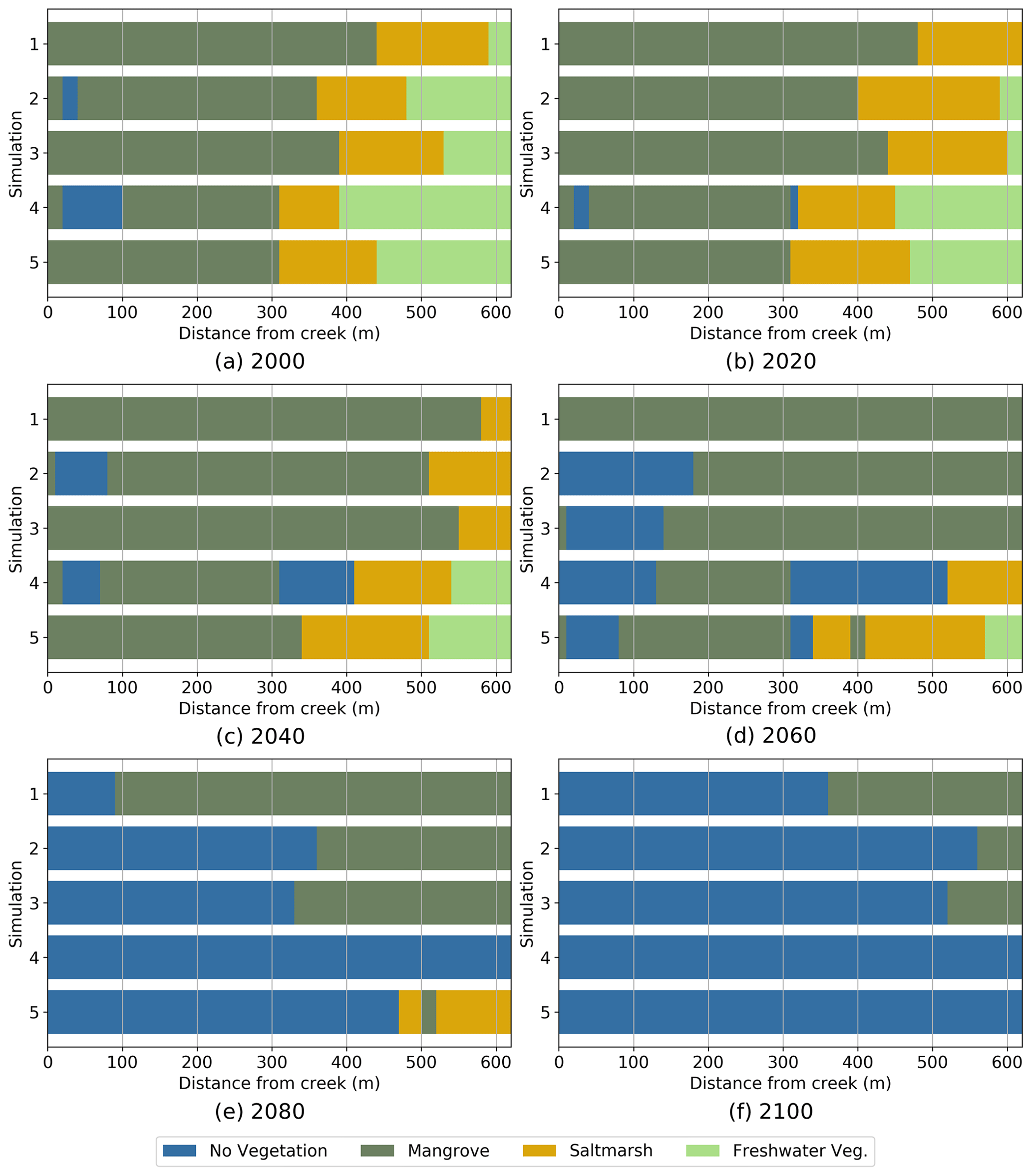
Figure 5 Predominant position occupied by each vegetation type in the tidal flat from 2000 to 2100. Simulations for low sediment input, $\mathrm{SSC}=\mathrm{37}\mathrm{g}{\mathrm{m}}^{-\mathrm{3}}$. Simulations: 1 Bathtub, 2 Free tidal flat, 3 Inner channel, 4 Embankment with culvert and 5 Embankment and inner channel.

After 20 years (Fig. 5b) Simulations 1, 2 and 3 show mangrove encroachment on saltmarsh. The upstream mangrove edge moves up to 50 m, forcing saltmarsh occurrence in areas further than 300 m from the tide input creek. In Simulations 4 and 5 the embankment halts mangrove migration and increases in inundation of upper areas promote saltmarsh increase. Overall, wetland area increases due to mangrove expansion (Simulations 1, 2 and 3) or to saltmarsh expansion (Simulations 4 and 5).

By 2040 (Fig. 5c), mangrove has encroached further on saltmarsh in Simulations 1, 2 and 3, resulting in saltmarsh squeeze at the upper end due to the landward boundary of the computational domain. Simulations 4 and 5 show very minor encroachment of mangrove on saltmarsh, which is able to migrate landward. Total wetland area remains approximately unchanged for Simulations 1, 2 and 3, while it keeps increasing in Simulations 4 and 5. Some areas of mudflat start appearing in the HST simulations due to extended hydroperiods.

Twenty years later, in 2060 (Fig. 5d), the MSL is about 30 cm higher than in 2000, and we can see considerable mudflat areas in all simulations except for the bathtub simulation (Simulation 1), which presents a uniform coverage of mangrove over the entire domain. Saltmarsh is totally absent in Simulations 1, 2 and 3 due to mangrove encroachment but still remains almost unchanged in Simulations 4 and 5. All simulations except the bathtub simulation show decreases in wetland extent, mostly due to saltmarsh disappearance in Simulations 2 and 3 and to mangrove squeeze in Simulations 4 and 5.

From 2080 on (Fig. 5e, f), a rapid retreat of the remaining wetland can be observed in all simulations. The retreat occurs faster for the simulations with the embankment, resulting in total wetland disappearance by 2100. The rest of the simulations still show some remnant mangrove areas by 2100, which are only significant (40 %) in the case of the bathtub simulations.

The same trend of increase in wetland area in the first 20 years of simulation, followed by a continuous decrease starting at 40 years and ending at 100 years with almost complete wetland disappearance under the same sea-level rise trajectory, was observed by Rodriguez et al. (2017) and Sandi et al. (2018). Sandi et al. (2018) also reported larger wetland losses in their simulations with tidal input restrictions at the wetland inlet when compared to the case without restrictions.

The same analysis of vegetation evolution for the high sediment input scenario is presented in Fig. 6. With increased sediment, the patterns of vegetation change remain remarkably similar to the patterns observed in Fig. 5 for the low sediment conditions, with the exception of the bathtub simulations (Simulation 1). Compared to Fig. 5, the bathtub results indicate that saltmarsh is able to remain in the upper wetland areas for longer (until 2060) and that mangrove does not retreat, resulting in no wetland loss after 100 years of simulation. The other simulations without embankment (2 and 3) show a slightly slower retreat of both mangrove and saltmarsh than in Fig. 5, while the simulations with the embankment show almost the same behaviour as in the case of low sediment. Some of the simulations in Fig. 6 show localised mangrove areas that tend to establish themselves and persist close to the tidal creek.

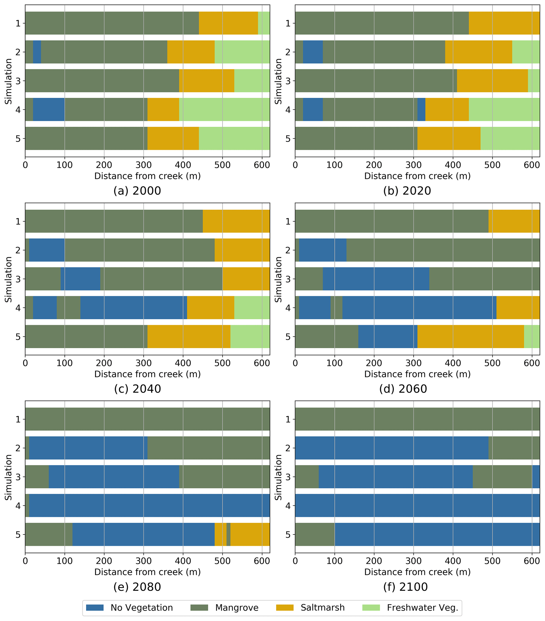
Figure 6 Predominant position occupied by each vegetation type in the tidal flat from 2000 to 2100. Simulations for high sediment input, $\text{SSC}=\mathrm{111}\mathrm{g}{\mathrm{m}}^{-\mathrm{3}}$. Simulations: 1 Bathtub, 2 Free tidal flat, 3 Inner channel, 4 Embankment with culvert and 5 Embankment and inner channel.

For a more detailed analysis, we can look at the vegetation evolution in terms of wetland area (mangrove and saltmarsh), wetland retreat (position of the seaward edge) and wetland transgression (position of the landward edge).

Figure 7a shows that the wetland extent predicted using the bathtub approach (Simulation 1) is affected by the sediment load, with only the low sediment condition resulting in a sharp decay in extent after 2060/70. The difference in extent is due to the vegetation retreat in the low sediment case, which does not occur in the high sediment case (Fig. 7b). Wetland extent values for the HST simulations are not greatly affected by the sediment load, and they are much smaller than the values predicted by the bathtub (Fig. 7a). Wetland retreat starts first in the simulations without the channel (Simulations 2 and 4) and about 20 years later in the simulations with the channel (Simulations 3 and 5) due to increased drainage. Once the retreat starts, it occurs faster in the simulations with the embankment (Simulations 4 and 5) that delays the ebb flows and increases hydroperiods in the lower wetland areas.

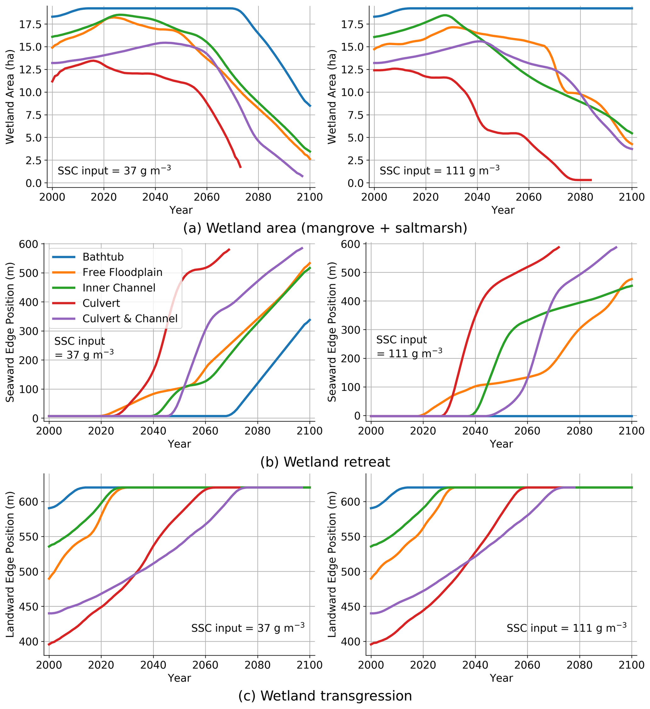
Figure 7 Time evolution of wetland in low ($\text{SSC}=\mathrm{37}\mathrm{g}{\mathrm{m}}^{-\mathrm{3}}$) and high ($\text{SSC}=\mathrm{111}\mathrm{g}{\mathrm{m}}^{-\mathrm{3}}$) sediment environments under SLR. (a) Wetland area; (b); wetland retreat; and (c) wetland transgression.

Wetland transgression is not affected by the sediment conditions (Fig. 7c) because of the limited amount of sediment that reaches the upper wetland areas. Transgression starts later in the simulations with the embankment (Simulations 4 and 5) because of the reduced depths and sediment loads in the upper wetland areas. The presence of the channel (Simulations 3 and 5) results in earlier but more gradual transgression compared to setups with no drainage structure (Simulations 2 and 4).

4 Discussion

The interactions between all the processes related to the dynamics of coastal wetlands are quite complex (Fagherazzi et al., 2012; Reef et al., 2018; Saintilan et al., 2014), which makes the bathtub assumption limited for most applications. Places with multiple vegetation species (Cahoon et al., 2011; Rogers et al., 2006) and an intertwined channel network (D'Alpaos, 2011) present a strong heterogeneity of saltwater exposure and sediment delivery to the overbank areas that need a detailed description of flow and sediment processes (see also Coleman et al., 2020). Artificial structures constraining flow and sediment modify accretion rates (Bellafiore et al., 2014; Cahoon et al., 2011) and thus wetland evolution (Rodriguez et al., 2017; Sandi et al., 2018). Even though our simulation design focused on simplified setups, these setups comprise typical wetland features and include most of the complex processes and interactions.

Our results indicate that wetlands do not cope with SLR for the simulated conditions corresponding to a high-emission climate change scenario. This result was not surprising for the low sediment situation, as the inability of sediment-poor coastal wetlands to survive high levels of SLR due to low accretion rates has been reported before (Kirwan et al., 2010; Lovelock et al., 2015b; Rodriguez et al., 2017; Sandi et al., 2018; Schuerch et al., 2018). However, the results for high sediment load seem to challenge some previous studies highlighting the potential of biophysical feedbacks to produce accretion rates comparable to SLR (D'Alpaos et al., 2007; Kirwan and Murray, 2007; Kirwan et al., 2016b; Mudd et al., 2009; Temmerman et al., 2003). In our case, the biophysical feedbacks with a high sediment load produced wetland accretion rates similar to SLR rates only for the bathtub simulation.

Analysis of accretion rates indicates that all simulations start with similar rates in the vegetated areas, with about 2.5 and 7.5 mm yr⁻¹ in the low and high sediment situations respectively. For the low sediment case, the initial value compared very well with historic values for south-eastern Australian conditions measured by Howe et al. (2009) and Rogers et al. (2006). For the high sediment case, an increase in the accretion value by a factor of 3 seems reasonable considering an increase in the sediment load by a factor of 3 (from 37 to 111 g m⁻³). Those starting values of accretion remain at approximately the same level over most of the time for the bathtub simulations, while they decrease for the HST simulations. The decrease is more marked for Simulations 2 and 4 (which reach a value of about 1 to 1.5 mm yr⁻¹ by 2050) than for the simulations with inner channel Simulations 3 and 5 (which attain values of 2 and 4 mm yr⁻¹ by 2050 for low and high sediment conditions respectively). The reduction of the magnitude of the biophysical feedbacks over time is due to the continuous upland migration of vegetation, which colonises upper areas with comparatively less water depth and sediment supply (see also Sandi et al., 2018). The bathtub model predicts less migration and higher depths, so it consistently overestimates accretion rates.

Despite having reduced accretion rates when compared to the bathtub simulations, the HST simulations still show a noticeable difference in elevation gains depending on the sediment supply levels. Compared to the low sediment case, the high sediment supply case results in about twice the average accumulated accretion (Fig. 4). However, analysis of vegetation changes over time for low (Fig. 5) and high (Fig. 6) sediment loads reveals minimum differences between them. Analysis of Fig. 7 shows that even though the increase in sediment load generates about twice the accretion, this extra elevation is not sufficient to prevent wetland submergence. Figure 4 suggests that accretion rates of 4 times the historic values or more are needed for the wetlands to be able to cope with SLR.

Although the simulations carried out in this study were conducted on simplified domains, they can capture the general response of more complex domains present in real wetlands, as shown by the comparison with entire wetland results from Rodriguez et al. (2017) and Sandi et al. (2018) in Fig. 4. Moreover, the features included are present in many coastal areas around the world and thus have wider implications. Our bathtub results for low sediment conditions predicting an initial increase in wetland extent early in the century and then a decrease after 2060 agree with previous bathtub model predictions (Lovelock et al., 2015b; Rogers et al., 2012; Schuerch et al., 2018). However, using the HST framework, our predictions indicate that the decrease may start as early as 2030 for wetlands with a tidal range close to 1.3 m (as represented in our study), over a wide range of sediment loads. We can expect that this accelerated wetland loss will affect many parts of the world, particularly in areas with micro to meso tidal ranges and heavily developed coasts, like eastern Australia (Williams and Watford, 1997), parts of the eastern US (Crain et al., 2009), the western US (Thorne et al., 2018), eastern China (Tian et al., 2016) and western Europe (Gibson et al., 2007). In these environments, attenuation can be important due to manmade structures, and transgression may be limited by development (Doody, 2013; Geselbracht et al., 2015; Kirwan and Megonigal, 2013), so we can expect a behaviour closer to that of Simulations 4 and 5. On the other hand, wetlands with dense drainage networks like the Venice Lagoon in Italy (Silvestri et al., 2005), the Scheldt estuary in the Netherlands (Temmerman et al., 2012), and the North Inlet in South Carolina, US (Morris et al., 2005), would probably behave similarly to Simulation 3 and experience comparatively smaller losses of area.

The results presented in this study show generalised conditions of wetland dynamics under sea-level rise by using several simplified domains that focus on individual mechanisms affecting ecogeomorphic evolution. This approach can support a broader perspective of the potential fate of coastal wetlands in general, but some limitations arise as part of the model assumptions. As with most wetland evolution models, we did not consider soil processes other than accretion, disregarding swelling, compaction and deep subsidence. Measurements in wetlands of the Hunter estuary show that long-term surface elevation changes are mostly due to accretion, supporting our assumption (Howe et al., 2009; Rogers et al., 2006). Another process that we did not consider was the effects of marsh edge retreat due to ocean or wind waves (Carniello et al., 2012; Fagherazzi et al., 2012), which can have a significant role in coastal wetland evolution. Most coastal wetlands in Australia are estuarine and not exposed to ocean waves, whereas wind effects in our wetland were not important due to the absence of large open water areas where wind waves could fully develop. We also simplified the tidal signal without including neap–spring cycles, which sped up computations but which may have affected the results. However, preliminary tests including neap–spring tide variability showed only small differences in the initial landward edge of saltmarsh, which did not affect the accretion dynamics due to the small depths and low sediment availability in that area. Finally, our simulations did not include the effect of storms, which can influence sediment availability, water depths and velocities. We believe that in our case excluding storm effects is justifiable based on Rogers et al. (2013), who found that in these fine sediment environments storms affect accretion dynamics over the short term (immediate erosion or low accretion followed by increased deposition over the next months), but they do not change the long-term trend of accretion and elevation gain rates.

5 Conclusions

We conducted detailed numerical simulations on the response to SLR of four different typical coastal wetland settings, including the case of a vegetated tidal flat free from obstructions and drainage features and three other settings that included an inner channel, an embankment with a culvert, and a combination of inner channel, embankment and culvert. We also included a simulation using a simple bathtub approach, in which none of the features (vegetation, channels, culverts) are considered. We used conditions typical of south-eastern Australia in terms of vegetation, tidal range and sediment load, but we also analysed simulations with an increased sediment load to assess the potential of biophysical feedbacks to enhance accretion rates.

We found that the distinct patterns of flow and sediment redistribution obtained from these simulations result in increased wetland vulnerability to SLR when compared to predictions using the simple bathtub approach. Changes in elevation due to accretion were between 10 % and 50 % of those obtained from bathtub predictions, and wetland retreat and reduction of wetland extent started 20 to 40 years earlier than for the case of the bathtub simulations, depending on wetland setting. Transgression for all settings was delayed with respect to the bathtub predictions and was limited by the presence of a hard barrier at the upland end.

The simulations using the full hydrodynamic and sediment transport dynamic models indicated that wetlands with good drainage (e.g. including an inner channel) were more resilient to SLR, displaying more accretion, a later retreat and reduction of wetland area and an increased transgression when compared with wetlands with strong flow impediments (e.g. including an embankment).

Increasing the sediment load delivered to the wetlands by a factor of 3 increased the accretion of all wetland settings by a factor of 2. However, this extra elevation was not enough to prevent wetland submergence, as predictions of wetland evolution were very similar for low and high sediment conditions. Based on our results, we estimate that accretion rates of 4 times the typical historic values or more would be needed for these wetlands to cope with SLR.

Even though the characteristics of the wetlands studied here correspond mainly to south-eastern Australian conditions, our results have a wider relevance because they clearly link the capacity of wetlands to accrete and migrate upland, the two mechanisms by which wetlands can gain elevation and keep up with SLR. Failure to consider the spatial coevolving nature of flow, sediment, vegetation and topographic features can result in overestimation of wetland resilience. Our results reconcile the wide discrepancy between upper thresholds of wetland resilience to sea-level rise in previous modelling studies with those emerging from paleo-stratigraphic observations.