the Creative Commons Attribution 4.0 License.
the Creative Commons Attribution 4.0 License.
 | 17 Feb 2021
The challenges of an in situ validation of a nonequilibrium model of soil heat and moisture dynamics during fires
William J. Massman
With the increasing frequency and severity of fire, there is an increasing desire to better manage fuels and minimize, as much as possible, the impacts of fire on soils and other natural resources. Piling and/or burning slash is one method of managing fuels and reducing the risk and consequences of wildfire, but the repercussions to the soil, although very localized, can be significant and often irreversible. In an effort to provide a tool to better understand the impact of fire on soils, this study outlines the improvements to and the in situ validation of a nonequilibrium model for simulating the coupled interactions and transport of heat, moisture and water vapor during fires. Improvements to the model eliminate the following two important (but heretofore universally overlooked) inconsistencies: one that describes the relationship between evaporation and condensation in the parameterization of the nonequilibrium vapor source term, and the other that is the incorrect use of the apparent thermal conductivity in the soil heat flow equation. The first of these made a small enhancement in the stability and performance of the model. The second is an important improvement in the physics underpinning the model but had less of an impact on the model's performance and stability than the first. This study also (a) develops a general heating function that describes the energy input to the soil surface by the fire and (b) discusses the complexities and difficulties of formulating the upper boundary condition from a surface energy balance approach. The model validation uses (in situ temperature, soil moisture and heat flux) data obtained in a 2004 experimental slash pile burn. Important temperature-dependent corrections to the instruments used for measuring soil heat flux and moisture are also discussed and assessed. Despite any possible ambiguities in the calibration of the sensors or the simplicity of the parameterization of the surface heating function, the difficulties and complexities of formulating the upper boundary condition and the obvious complexities of the dynamic response of the soil's temperature and heat flux, the model produced at least a very credible, if not surprisingly good, simulation of the observed data. This study then continues with a discussion and sensitivity analysis of some important feedbacks (some of which are well known and others that are more hypothetical) that are not included in the present (or any extant) model, but that undoubtedly are dynamically influencing the physical properties of the soil in situ during the fire and, thereby, modulating the behavior of the soil temperature and moisture. This paper concludes with a list of possible future observational and modeling studies and how they would advance the research and findings discussed here.
- Article
(13999 KB) - Full-text XML
- BibTeX
- EndNote


This paper was written and prepared as part of my official duties as a US government employee. It is, therefore, in the public domain and may not be copyrighted.
Fire has been a largely beneficial part of the landscape in most areas of the world for millennia (Harrison et al., 2010). But, over the past few decades, fire has increased significantly in frequency, extent and severity – to the point that it now poses substantial risks to most of the world's wildlands and forested ecosystems and the goods and services they provide (e.g., Kasischke and Turetsky, 2006; Mortiz et al., 2012; Abatzogloua and Williams, 2016; Stambaugh et al., 2018; San-Miguel-Ayanz et al., 2019). Consequently, there is an increased desire to reduce wildfire risk through better fuels management, mitigate the consequences of fire by improving management methods, and promote the recovery of soils and vegetation after fire (e.g., Millar et al., 2007; McCaffrey et al., 2015; Vallejo and Alloza, 2015; Schoennagel et al., 2017; Dey and Schweitzer, 2018). Therefore, to achieve any of these desired outcomes for managing the ecological effects of fire, it is necessary to improve our understanding of the impacts that fire and extreme heating can have on soils. An important and extremely useful tool in this effort is having better models of soil heating during fires. The benefit of a model lies in its ability to vary the amount and duration of heating (e.g., Steward et al., 1990) that characterize different fire types and to better judge how fire impacts different soil types. And, just as there are a variety of different soil types with differing thermophysical properties, there are also a variety fire types characterized by duration, intensity and, for the present purposes, the ability to heat the soil's surface, i.e., the soil heat flux (W m−2). For example, the prescribed burning of understory vegetation, which is an example of spreading or dynamic fire used to reduce understory fuels, is usually low intensity and will heat the soil for only a few minutes. But as the fuel loading increases, so does the fire's duration and intensity (e.g., Massman et al., 2003). On the other hand, prescribed slash pile burns, like the one studied here, are stationary fires that can that can sustain a soil heat flux of 1–10 kW m−2 for tens of hours (e.g., Massman and Frank, 2004; Massman et al., 2008). Wildfires, and crown fires in particular, are dynamic and often fast moving and relatively brief by comparison to slash pile burns, but they can also be extraordinarily intense (10–100 kW m−2). Yet, despite their often extreme intensity, dynamic fires can produce a counterintuitive spatial pattern of soil surface heating, i.e., negligible heating near the region of the most intense fire to significant heating in areas of much lower fire intensity (Stoof et al., 2013). It is also possible that a fast-moving crown fire can cause burning material, e.g., tree boles or other woody material, to come into direct contact with the soil, producing a stationary fire that can continue to burn or smolder long after the fire front itself has passed. With the present modeling approach, it makes it relatively easy (just by changing the model's soil surface boundary forcing) to estimate the depth of penetration of critical temperature thresholds (e.g., Massman et al., 2010a, Fig. 1) for differing soil types. Here I summarize the changes made to the HMV (Heat–Moisture–Vapor) model (Massman, 2015) and assess the improvements they made to the model's performance by comparing modeled and observed (in situ) soil temperatures, heat fluxes and changes in soil moisture during a 2004 slash pile burn (Massman et al., 2008). Note that this model has been tested on several other instrumented slash pile burns and a few dynamic wildfires and controlled laboratory fires. Although the results will not be presented here (principally because the large majority of these fires were not instrumented with in situ soil moisture probes), these other fires did provide insights into soil heating dynamics during the fires and additional tests for building confidence in the model's performance.
The HMV model is a 1D (soil depth) model with three time-dependent predictive variables, namely temperature, TK (K) or T (∘C), soil water potential, ψ (J kg−1) (where ψ<0 and is relatable to volumetric soil moisture θ (m3 m−3) through a water retention curve), and soil vapor density, ρv (kg m−3). At any specific depth, the model assumes thermal equilibrium between the soil matrix, the soil vapor and the soil moisture. However, it is termed a nonequilibrium model because it does not assume a priori that the soil moisture and soil vapor are in equilibrium, contrary to the equilibrium approach that has been the basis of virtually all models of coupled heat and moisture flow in soils since Philip and de Vries (1957) and de Vries (1958). Although the equilibrium assumption has led to many insights into the nature of soil heat and moisture transport processes in the last six decades, it must fail at some point as the soil dries out for the simple reason that it is difficult to maintain vapor in equilibrium with soil moisture when there is little to no soil moisture (Novak, 2012; Massman, 2015). In the case of rapid soil heating and drying during fires, Massman (2015) further indicates that at the drying front, where local soil evaporation rates are highest, θ and ρv are forced out of equilibrium as soil moisture rapidly decreases and the soil vapor rapidly increases. Novak (2019) also demonstrates (under less extreme conditions than during fires, i.e., ∘C) that the greatest departure from equilibrium occurs at the drying front. The equilibrium model cannot capture this evaporative disequilibrium, which may explain why soil evaporation is better modeled with a nonequilibrium approach (Smits et al., 2011; Ouedraogo et al., 2013; Massman, 2015; Borujerdi et al., 2019). In fact, the most important change/improvement in the HMV model (detailed in the next section) is in the parameterization of the vapor source term, Sv (kg m−3 s−1), which is the essence of the nonequilibrium approach and its ability to capture the evaporative disequilibrium. As with its predecessor (Massman, 2015), the present vapor source term is formulated on the basis of the Hertz–Knudsen equation, which Trautz et al. (2015) have suggested describes evaporation better than other nonequilibrium models of Sv. Nonetheless, all extant models of Sv have overlooked (and therefore include) an implicit and incorrect assumption about soil evaporation that is addressed and corrected in the present study.
The following section also discusses other changes in the HMV model, including (a) eliminating the use of the apparent soil thermal conductivity in the soil heat flow equation (also further discussed and justified in the Appendix), and (b) improving the parameterization of the surface energy balance and the upper (soil surface) boundary condition (including the development of a generic soil heating function for use with prescribed burns or wildfires). In addition, this study also discusses the subtleties and difficulties of formulating a universal surface energy balance for soil heating by fire. The third section reviews the site, soils and data of the experimental slash pile burn, and the fourth section compares the observations with the model simulations and explores some of the consequences (to the simulations) of some dynamic feedbacks and interactions between the fire and soil physical properties. The fifth section discusses possible future directions for modeling and observational studies. The final section summarizes this study.
Similar to version 1 of the HMV model (Massman, 2015), the present version employs a linearized Crank–Nicolson finite difference scheme and was coded and run using MATLAB version 2017b. This paper also uses the same notation and the same functional parameterizations for the supporting thermodynamic and physical variables as Massman (2015). For this study, details concerning these functional parameterizations will be summarized, as necessary, for clarity and will be updated with new information or data. Otherwise, many details covered by Massman (2015) will not be repeated here. The remainder of this section discusses the physical fundamentals of the changes made to the HMV model.
2.1 Conservation of mass and energy
The HMV model is composed of the three conservation equations, namely the conservation of energy (or maybe more properly the conservation of enthalpy), the conservation of soil liquid water and the conservation of soil water vapor. The conservation of energy is as follows:
where Cs (J m−3 K−1) is the volumetric specific heat of the soil, such that is a function of both temperature and volumetric soil moisture. t (s) is time, z (m) is soil depth, and λs (W m−1 K−1) is soil thermal conductivity, such that ; Lv=Lv(TK) (J kg−1) is the enthalpy of vaporization and −LvSv represents the change in enthalpy associated with evaporation/condensation. is the source term for water vapor and is discussed in more detail in the following section. WSw is the change in enthalpy associated with the heat of wetting (also termed the heat of immersion), where W (J kg−1) is the heat of wetting and Sw (kg m−3 s−1) is the source term for water liquid, or equivalently the sink term for water vapor, i.e., . W is discussed by de Vries (1958) and, for the present purposes, W can be interpreted as that additional enthalpy of vaporization that is required to break the electrostatic bonds between molecular water and the soil mineral surfaces. In general, the wetting reaction is exothermic, i.e., W>0, and a function of temperature (Grant, 2003; Prunty and Bell, 2005). Massman (2012) investigated the effects of temperature on ψ and W but found that it had little impact on the modeling results. For this study, the HMV model follows Campbell et al. (1995) and assumes that and ignores any temperature dependencies of ψ and W. Note that W is only significant at high temperatures (as Lv→0) and for extremely dry soil (as ). Finally, with this identification for W and the above identity between Sw and Sv, it follows that .
The conservation of liquid water is as follows:
where ρw=ρw(TK) (kg m−3) is the density of liquid water, and ψn (dimensionless) is the nondimensional form of ψ, i.e., , where J kg−1 is the nominal soil water potential of ovendried soil (Campbell et al., 1995). (Note that ψn is used interchangeably with ψ throughout this paper.) (m2 s−1) is the hydraulic diffusivity, (m s−1) is the hydraulic conductivity, and (m s−1) is the velocity of liquid water associated with surface diffusion of water. The hydraulic conductivity functions, and , are given as follows:
where μw=μw(TK) (Pa s) (Huber et al., 2009) is the viscosity of water, and g=9.81 m s−2 is the acceleration due to gravity. KI (m2) is the intrinsic permeability of the soil – here assumed to be constant and uniform throughout the soil profile but does, in fact, vary with the concentration and type of solutes in soil water, (e.g., Lutz and Kemper, 1959). (dimensionless) is the relative hydraulic conductivity (used to describe capillary flow in soils). The model for intrinsic permeability is taken from Bear (1972) and is , where dg (m) is the mean or effective soil particle diameter. Note that switching variables from ψ<0 to ψn produces ψn>0 and Kn<0. The present model considers only capillary flow and will ignore film flow because, as in Massman (2015), film flow did not really impact the model's performance.
The conservation of water vapor is as follows:
where η (m3 m−3) is the total soil porosity, assumed to be temporally constant and spatially uniform (note that η is obtained from the soil's bulk and particle densities, which are the actual model input variables, and because both of these variables are assumed constant and uniform, so also is η), and (η−θ) is the soil's air filled porosity. (m2 s−1) is the (equivalent) molecular diffusivity associated with the diffusive transport of water vapor in the soil's air-filled pore space, where Dve includes the enhancement factor, developed by Campbell et al. (1995) and detailed in Massman (2012). uvl (m s−1) is the advective velocity induced by the change in volume associated with the rapid volatilization of soil moisture (e.g., Ki et al., 2005), which is given as follows:
The final model equations result from preserving Eq. (4) and eliminating Sv from Eqs. (1) and (2), such that Eq. (1) is replaced with the following:
and Eq. (2) is replaced with the following:
2.2 Improvements in nonequilibrium vapor source term
Massman (2015, Equation (10)) adapted the Hertz–Knudsen equation to develop the following formulation for the vapor source term, Sv:
where S* is an empirical dimensionless parameter, which is tuned as necessary to ensure model stability. Awa (m2 m−3 or m−1) is the volume-normalized soil water–air interfacial surface area, which Massman (2015) parameterized as Awa=Awa(θ). R=8.314 J mol−1 K−1 is the universal gas constant, Mw=0.01802 kg mol−1 is the molar mass of water vapor, and 𝒦e (dimensionless) is the mass accommodation (or evaporation) coefficient, which Massman (2015) sets ≡1. (dimensionless) is the thermal accommodation (or condensation) coefficient, which Massman (2015) parameterizes as a physicochemical (Arrhenius) function as follows: , where Eav−Mwψ (J mol−1) is an empirical surface condensation/evaporation activation energy for which Eav≈30–40 kJ mol−1 was determined empirically, and TK,in is the initial soil temperature. ρv,eq (kg m−3) is the equilibrium vapor density, defined as , where is the dimensionless water activity, modeled here with the Kelvin equation, and ρv,sat(TK) (kg m−3) is the saturated vapor density, which is a function only of TK.
But the model of Sv, embodied by Eq. (8), assumes that the interfacial surfaces appropriate for evaporation and condensation are the same, i.e., that Awa is the same for both evaporation and condensation . In general, this is not a priori the case, unless one assumes that soil moisture (θ) never drops below the point at which the soil's interfacial surface area is completely covered by a thin film or monolayer of liquid water (e.g., Novak, 2019). But it is physically more realistic, at least for very dry soils (which are likely to occur during fires), to assume that condensation can occur even in the absence of liquid water. Otherwise models of Sv would impose a physically unrealistic constraint on nonequilibrium models of heat and moisture flow in dry soils.
The new version of the nonequilibrium model parameterizes Sv as follows:
where 𝒦e≡1 has been retained – as has the original formulation for Awa (Massman, 2015), as follows:
where is the soil water saturation and a1=50 (rather than the original value of 40), a2=0.003 and . This particular value for the parameter a1 was chosen so that the maximum value of Awa occurs at 𝒮w≈0.02 () and is assumed to be where the soil surfaces are covered by a monolayer of water (Brusseau et al., 2006). , as long as , and whenever . In other words, Awa,dry differs from Awa whenever the soil moisture is so low that the soil particle surfaces are covered by, at most, a monolayer of water. Empirical tuning of S* and Eav, after implementing the other changes, yielded and Eav=10 kJ mol−1. Together, these changes in Sv improved the model's stability and robustness and its fidelity to the observed soil moisture during the 2004 burn (detailed later).
2.3 Corrections and improvements in soil thermal conductivity
The present model of λs retains (a) the general structure of the original Campbell–de Vries model for thermal conductivity (see Campbell et al., 1994; de Vries, 1963; Massman, 2012) and (b) the additional Bauer term associated with the high-temperature thermal (infrared) radiant energy transfer within the soil pore space (Bauer, 1993). That is, in the following:
where kw, ka and km (dimensionless) are the Campbell et al. (1994) generalized formulations of the de Vries (1963) weighting factors. λw(TK,ρw) (W m−1 K−1) is the thermal conductivity of liquid water, and (W m−1 K−1) is the apparent thermal conductivity of moist air, which is the sum of the true thermal conductivity of moist air, (W m−1 K−1) and the term, (W m−1 K−1), which embodies the effects of latent heat transfer or “the effect of the vapor distillation due to temperature gradients” (de Vries, 1958; Appendix A of the present study). λm (W m−1 K−1) is the thermal conductivity of the mineral components of the soil, σ (W m−2 K−4) is the Stefan–Boltzmann constant, (dimensionless) is the pore gas index of refraction, and Rp (m) is the soil's pore space volumetric radius. The first term on the right-hand side of Eq. (11) is the Campbell–de Vries model and the second is the Bauer term.
The weighting factors, kw, ka and km, all have the same general form (Campbell et al., 1994), as follows:
where the subscript * refers to water (w), air (a) or mineral (m). ga is the de Vries (1963) shape factor, an empirically determined model parameter. In general, ga≈0.1 (Campbell et al., 1994). is a weighted mixture of the thermal conductivities of air and water as follows:
and
where qw(TK) is a dimensionless parameter that describes the water content at which water begins to influence λs. It is defined as with qw0, another empirically determined parameter. ga and qw0 are important for the present study because they are an important part of the sensitivity analysis (discussed in a later section) that explores the interactions between the fire and the soil physical properties.
A total of three changes have been made to this original formulation. First, is no longer included because to do so is to double count the vapor “distillation” (de Vries, 1958) term that accounts for the influence that evaporation, transport and condensation of water vapor can have on the apparent thermal conductivity (Appendix A). In other words, as shown in Appendix A, both equilibrium and nonequilibrium models of soil heating include the vapor distillation term, either explicitly through the conservation of mass of water vapor (nonequilibrium models) or implicitly through the conservation of mass of liquid water (equilibrium models). Consequently, it is unnecessary and redundant to include in Eq. (11).
Second, λm now includes an explicit temperature dependency of the form , where λm0 (W m−1 K−1) is basically an adjustable parameter. The results for α quartz (α referring to a specific crystalline structure of quartz) from (Yoon et al., 2004, Fig. 4) suggests that it is reasonable to expect that λm0≤15 W m−1 K−1. The temperature function was chosen to emulate the approximately 70 % decrease in the thermal conductivity of α quartz (here used as a substitute for sand quartz) between about 300 and 600 K, as shown by Kanamori et al. (1968) and Yoon et al. (2004). At the Manitou Experimental Forest (MEF) burn site, and more generally throughout the region surrounding MEF, sand quartz is likely to be the dominant soil mineral, but other crystalline mineral forms, such as granite and feldspar, are also common (e.g., Retzer, 1949; Mathews, 1900; Smith et al., 1999). Although the thermal conductivities associated with these other mineral forms also decrease with increasing temperature (Heuze, 1983; Mottaghy et al., 2008; Miao et al., 2014), overall they decrease with about half the slope () of the sand quartz parameterization used here. They also tend to show a much lower λm0 than quartz sand. Here λm0=4.42 W m−1 K−1, which should help accommodate these other nonsand quartz mineral forms.
Third, Rp is now estimated as from Arya et al. (1999), where dg (m) is the mean or effective soil particle diameter, ρp (Mg m−3) is the particle density (which can usually be assumed to be about 2.65 Mg m−3) and ρb (Mg m−3) is the soil bulk density. This formulation for Rp yields more physically realistic estimates of Rp (i.e., 5 µm ≤ Rp ≤ 200 µm for the soils tested in this study) than the default value of 1000 µm used in the previous version of the HMV model. It also suggests that the thermal infrared contribution to the soil thermal conductivity is negligible in most soils, even during fires. Massman (2015) reached a similar conclusion.
2.4 Evaluation of changes in Sv and λs
Assessing the consequences of these alterations to the source term and soil thermal conductivity to the model's performance was done using the laboratory data of Campbell et al. (1995) and by comparing the simulations with the changes in Sv and λs to those shown in Massman (2015). The results indicated that (a) the model's ability to faithfully reproduce the data was very similar to those in Massman (2015), and (b) the model's stability was noticeably improved. The reason for (b) is (almost exclusively attributable to) the change in Sv and is very much a positive benefit to the model. The changes in λs did require some adjustments to the values of some of the other parameters included in the model for λs, but these were minimal and not particularly significant. For the sake of brevity, none of these comparisons are included in this study.
2.5 Complexities and challenges
2.5.1 Surface heating, surface energy balance and upper boundary condition
The forcing function is the energy that is input to the soil at its surface, denoted here by QF(t) (W m−2). How that energy is divided between net infrared heat loss, convective heat loss, evaporation and soil conductive heating is expressed by the surface energy balance and the upper boundary conditions. Although relatively simple in concept, in practice, for application to fires, the forcing function, the surface energy balance and the upper boundary all are, at best, difficult to formulate precisely and, at worst, potentially a fiction. For example, in the case of a wildfire or soil heating within a few meters outside the physical perimeter of a slash pile, surface forcing is primarily radiant energy (see Fig. 2 of Massman et al. (2010a) for an example of this second case). On the other hand, when burning material makes direct contact with the soil, it is reasonable to assume that the forcing at the soil surface is more likely to be conduction rather than radiant energy. Beneath a burning slash pile, surface heating may be combination of radiation and conduction, it may change over time as the pile burns and as the ash accumulates and, at later stages of the burn, as the pile collapses. In the case of a moving fire front, the forcing can be highly variable. Radiant energy is clearly a major driver, but in addition, thermal instabilities drive circulations ahead and behind the fire that input energy into the soil when these circulations force hot air into contact with the soil, which, in turn, causes direct ignition of soil biomass ahead of the flame front (Finney et al., 2015; Pearce et al., 2019; Linn, 2019). As the fire front passes, the forcing is likely to be a combination of conduction and radiation and possibly convection, whereas, after the fire front, conduction is the major forcing in areas covered with burning biomass and radiant energy and possibly convection in areas free of burning biomass. Finally, in the case of burning duff, forcing is likely to be solely conductive in nature, but complications arise because, in this situation, duff is a highly porous burning insulator. Parameterizing the forcing in this case is problematic because of the extremely limited (empirical and theoretical) knowledge concerning burning duff.
Massman (2015) assessed the performance of the previous version of the HMV model against the laboratory data of Campbell et al. (1995), which more or less dictated the following forcing function: , where τ (s) and QFmax (W m−2) are adjustable parameters that describe the rate of rise of the forcing function (τ) and its steady state asymptotic (maximal) value QFmax. This study uses the following modified form of the “BFD curve” (Barnett, 2002) as the forcing function as follows:
where is the modified BFD curve, tm (s) is the time at which the maximum forcing occurs, α (dimensionless) = , and td (s) is the time interval between when the forcing first reaches 1% of its maximum and when it has decayed to 1 % of its maximum. QFmax, tm and td are adjustable input parameters to the model that define the forcing function, much the same way that QFmax and τ are for the Campbell et al. (1995) forcing function. QFin (W m−2), on the other hand, is not an adjustable input parameter. It is determined from other considerations of the soil surface energy balance and is defined later. The boundary conditions for temperature and vapor pressure, ev (Pa), have similar functional forms as Eq. (15) as follows: , where Va refers to the ambient atmospheric temperature (Ta) or vapor pressure (ρv,a) at the soil surface, and the subscript in refers to the initial value of that variable (taken from observations near the time and location of the fire). Vmax is an adjustable model input parameter that is tuned so that the model matches (as much as possible) the soil observational data and (if necessary) helps ensure model stability. The vapor density boundary condition is derived from these latter two boundary conditions using the ideal gas law. The upper boundary condition on soil moisture is and is discussed further in Massman (2015).
The energy balance at the soil surface used with the present study formulates the net infrared radiation loss at the surface as a balance between the outgoing and incoming infrared radiation. This is different from both Massman (2012) and Massman (2015), which did not include the possibility of incoming environmental infrared radiation being absorbed by the soil's surface. Here the surface energy balance is expressed as follows:
where the 0 subscript refers to soil surface, and the term on the left-hand side of this equation is the energy absorbed by the soil (and assumes that the absorptivity and emissivity of the soil are the same), and the first term on the right-hand side is the net infrared heat loss (where the term was not included in Massman (2012) or Massman (2015)). The second term is the convective heat loss, the third is the rate of evaporation and the last is the soil conductive heat. ϵ0(θ0) is the soil emissivity and is a function of the soil moisture, θ0. W m−2 K−4 is the Stefan–Boltzmann constant, ϵa(ρva) is the emissivity of the ambient atmosphere exposed to the soil surface during the fire and is a function of the ambient vapor density ρva, following the clear sky parameterization of Brutsaert (1984, Eq. (6.18)). (kg m−3) is the mass density of the ambient air at the soil surface temperature, TK0, where Pa (Pa) is the ambient pressure (at the time and location of the fire and is a model input variable) and PST=101 325 Pa and TST=273.15 K are the standard atmospheric pressure and temperature. CH=0.032 (m s−1) is the transfer coefficient for convective heat from the surface (see Massman, 2012 or Massman, 2015). Ta=Ta(t) (∘C), or equivalently TKa=TKa(t) (K), is the ambient temperature somewhere above the soil surface (upper boundary condition), (W m−2) is the rate of soil water evaporation, E0 (kg m−2 s−1) is the evaporative mass flux at the surface, and G0 (W m−2) is the soil conductive heat flux and the upper boundary condition for the modeled soil temperatures (Eq. 6). E0 is parameterized as the sum of a diffusional component and an advective component (Massman, 2012) as follows:
where CE (m s−1) and CU (dimensionless) are adjustable model transfer coefficients which were determined empirically to maximize E0 without destabilizing the model. CU=0.125 is associated with the jet of volatilized air emanating from the soil with velocity uvl0 and m s−1. The surface humidity, hs0 (dimensionless), is assumed to be the same as aw0, which is the water activity at the surface.
Although Eq. (16) completely accounts for the energy exchange between the atmosphere and the soil, there are two key issues that need to be addressed when initializing the model for applications to fires. The first was mentioned earlier; that is, under a burning slash pile or a soil covered (partially or completely) with an ash layer, it is not clear what the infrared and convective heat environments really are or what role they may play in the soil energy balance. Further complicating a proper formulation of the soil surface infrared (IR) and convective heat flow terms are the structure and porosity of the pile, which will influence the IR impinging on the soil surface, the airflow ventilating the pile interior, and the size and efficiencies of any convective eddies that may act to transfer heat toward or away from the soil surface. In this study, the upper boundary condition for temperature, Ta(t), is chosen to ensure that the convective heat flow is away from the soil surface. This issue is relevant here because the data used in this study was obtained under a burning slash pile, and it is addressed in the present study in a later section on sensitivity analysis by comparing model simulations with and without the IR and convective heat terms. Removing these later two terms from Eq. (16) yields the following simplified version of the soil surface energy balance:
The second issue is basically a feature of all forcing functions. In the case of the BFD curve, tm≥0.5 h is always true, and because a typical model time step is between 1 and 4 s, there will always an initial period between a few minutes to several tens of minutes long where the simulated burning time t≪tm. During this ramp-up period, QF≈QFin. The choice of QFin depends on whether Eq. (16) or Eq. (18) is used. In the case of Eq. (18), QFin=0. In this case, the soil conductive heat flux becomes , and because the source term and the evaporation rates are very nearly at equilibrium (i.e., Sv≈0 and E0≈0) during this ramp-up, it follows that G0≈0 and that . (Note that the soil is initialized to be isothermal at the temperature obtained at the soil surface just before initiating the burn.) But for Eq. (16), the full surface energy balance equation, this equilibrium condition does not occur during the ramp-up if QFin=0 because the net IR term in Eq. (16) is not initially in equilibrium. This is true despite initializing Ta=T0. Without QFin, Eq. (16) reduces to , which induces a transient in the solution that causes the soil temperature to drop slightly (i.e., ). But assigning eliminates this transient and ensures that G0≈0 and during the ramp-up time. Several other methods were tested for eliminating this unrealistic solution, but the present approach proved to be the least intrusive and the best way to prevent this initial transient. Note that this initial period of disequilibrium in the surface energy balance is not unique to the modified BFD curve. It also occurred with other forcing functions that were tested (e.g., Blagojević and Pešić, 2011) and with the Campbell forcing function used in Massman (2012) and Massman (2015).
2.5.2 The lower boundary condition and initial conditions
The lower boundary condition is the same pass-through or extrapolative boundary condition that was used in Massman (2012) and Massman (2015), i.e., the second derivative, , of the three model variables = 0. But, for the present study (which is devoted to wildfires and slash pile burns rather than the laboratory experiments of Campbell et al., 1995), the lower boundary is placed at 0.60 m below the surface (well below 0.20 m used in these previous studies). This pass-through boundary condition is used because, for field-based applications, the lower boundary condition will never be known (or knowable without extraordinary effort before hand), so it must be fairly general and placed at a depth where it will not influence the model predictions within the upper few centimeters of the soil too much. The advective velocity, uvl, requires only one boundary condition – see Eq. (5) – and is uvl=0 at the bottom boundary.
Although this combination of the pass-through lower boundary condition and placement depth (0.6 m) is fairly general, it is still possible that they may influence the model's solution within the region of greatest interest (the top 20 cm or so). To test for this possibility, a sensitivity test was performed by increasing the domain depth to 1 m. The resulting change in the model's solution was negligible throughout the upper 0.6 m. A total of two further simulations were done each with a zero-flux lower boundary condition for soil moisture (i.e., or, more specifically, ), where one had a domain depth of 0.6 m and the other had 1 m depth. The impact of these changes on the model simulation was, for the present purposes, also negligible. This zero-flux lower boundary condition for θ would seem to be a credible, but apparently unnecessary, and alternative to the present pass-through boundary condition, which is preferred here because it allows all model variables and their associated fluxes to be dynamically modeled. θ was chosen for this sensitivity analysis because it can be plausibly argued that there is enough known about a site's soil structure to make a credible guess at the depth at which the zero-flux boundary condition could be assumed. Soil temperature is better dynamically modeled at the lower boundary because the heat pulse for the fire can extend far deeper than 0.6 m, regardless of the soil structure (e.g., Massman and Frank, 2004). Finally, the pass-through formulation is also the logical default for vapor density because (a) ρv is more strongly controlled locally by the balance between evaporation and condensation than by the lower boundary condition, and (2) simply decreasing the effective vapor diffusivity, Dve , is sufficient for mimicking regions of highly impermeable soil without the need to explicitly incorporate a specific non-pass-through boundary condition.
The initial conditions for soil temperature and moisture are taken from measurements made just before igniting slash pile. The soil temperature is assumed to be uniform throughout the vertical domain and is taken to be the observed soil surface temperature. The initial soil vapor pressure is estimated to be about 40 % of the saturation vapor pressure at the initial soil temperature. The ideal gas law is then used to estimate the initial soil vapor density profile. The initial soil water potential is obtained from the soil moisture data using the water retention curve, which is discussed next.
2.6 The water retention curve
Unlike previous studies (Massman, 2012, 2015) which employed soils for which the water retention curve was unavailable, the present study employs a water retention curve appropriate to the soils at the MEF experimental burn site. Figure 1 shows the water retention curves (WRCs) for preburn (red) and postburn (black) soil. Note that both pre- and postburn soils are included in this study because they are part of the model sensitivity analysis. The data shown in this figure were provided by Gregory Butters (personal communication, 2009) and were obtained from a 2008 burn study performed at a site about 60 m away from the 2004 burn discussed in this study. The data were fitted with the Fredlund and Xing (1994) model as follows:
where a>0, b>0, n>0 and m>0 are fitting parameters, e is Euler's number, and the total porosity η was established beforehand, such that ηpre≈0.51 and ηpost≈0.45. These values of η correspond to the following values of soil bulk density: Mg m−3 and Mg m−3. This change in bulk density is revisited in the model sensitivity analysis. Although the Fredlund–Xing model provided the best fit to the data, other models of the WRC were fitted to the observations.
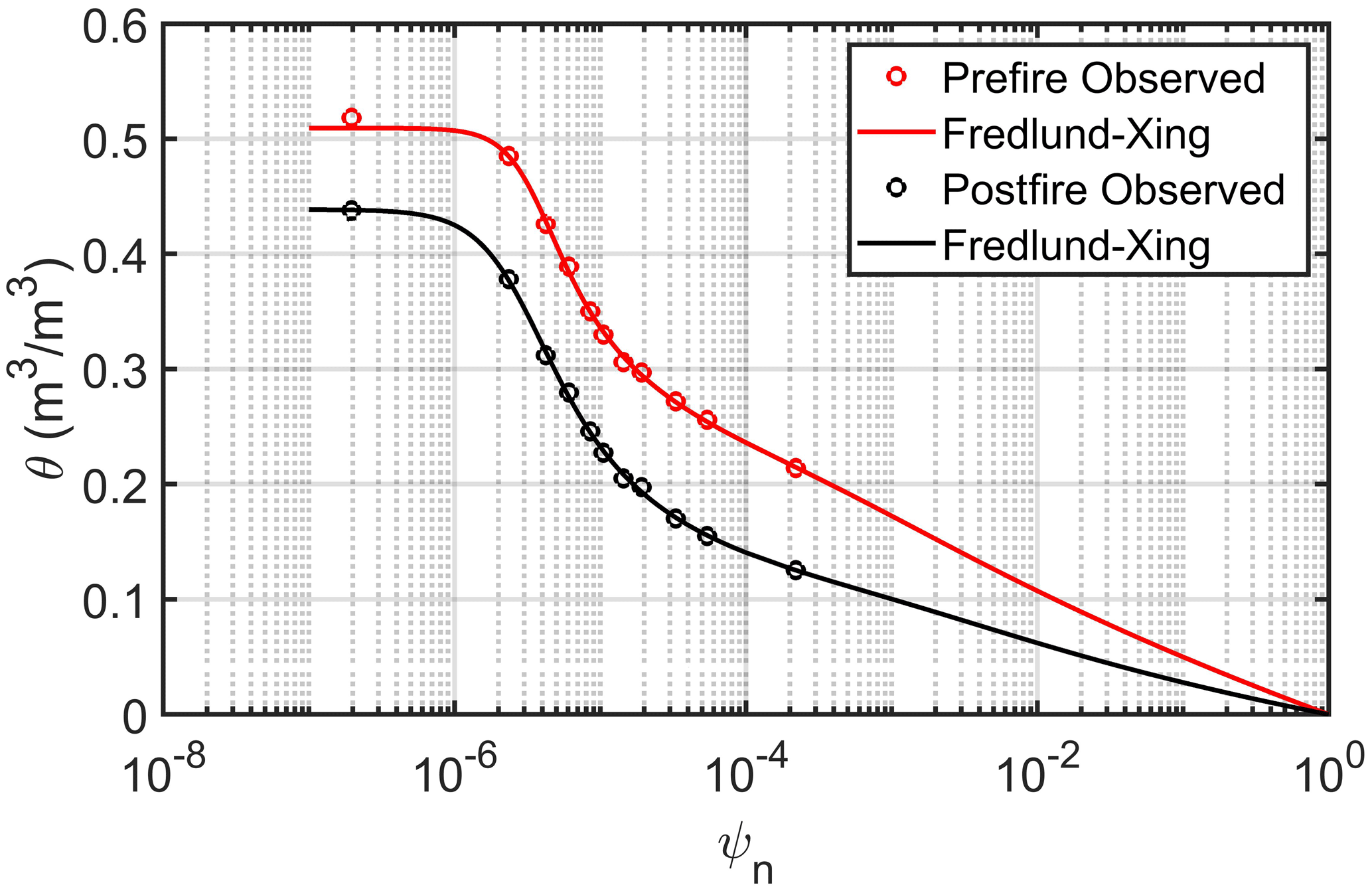
Figure 1Pre- and postburn water retention curves at the 2004 Manitou Experimental Forest (MEF) burn site. Observations were fitted with the Fredlund and Xing (1994) model. The only difference between these two curves is that the total or air-filled porosity is about 0.51 for the preburn (red), and it is about 0.45 for the postburn (black).
For the HMV model, the choice of WRC is important. The Fredlund–Xing model did provide the best fit to the data, and its impact on model performance was judged to be the best of the models tested. Other models for the WRC that were tested include the Campbell–Shiozawa model (Campbell and Shiozawa, 1992), which was used in both Massman (2012) and Massman (2015), the van Genuchten model (van Genuchten, 1980) and the Groenevelt–Grant model (Groenevelt and Grant, 2004). For the purposes of model performance, the key difference between Fredlund–Xing model, Eq. (19) and Campbell–Shiozawa model and (the class of models represented here by) the van Genuchten and the Groenevelt–Grant models is the WRC's description and mathematical behavior when the soil is extremely or completely dry. Under these conditions, Eq. (19) when θ≈0, the soil water potential remains bounded, i.e., J kg−1. But, with the van Genuchten and the Groenevelt–Grant models, a completely dry soil is impossible to achieve because θ=0 can only occur when . In the HMV model an unbounded function for the WRC does result in the degradation in model performance, i.e., some loss in the physical realism in the simulation of soil moisture, and can introduce model instabilities.
On the other hand, using a WRC that remains bounded produces a logical inconsistency when used with the Kelvin equation to describe water activity and the equilibrium vapor density. This issue plagued earlier modeling attempts (Massman, 2012, 2015). In the case of Massman (2012), when θ=0, J kg−1 and . But as long as the temperature keeps rising, , it follows that . For the equilibrium model (), this means that, when the soil moisture is completely evaporated and the soil is dry, the model autonomously creates water vapor. In the case of Massman (2015), the same inconsistency produces a source term that does not allow condensation to occur (i.e., Sv<0) on the surface of a soil particle that is completely dry. It is this issue that led to the improved parameterization of Sv embodied in Eq. (9) of the present study.
Additionally, temperature can also have significant effects on the WRC (e.g. Olivella and Gens, 2000; Salager et al., 2010), which is a consequence of the influence temperature has on the surface tension of water (σw=σw(TK) N m−1 (Vargaftik et al., 1983). Massman (2012) found that these effects were relatively small, even at very high temperatures, but his 2012 model did not include any possibility of soil water movement (i.e., KR=0). Milly (1984) includes the temperature effects on both the WRC (σw) and the hydraulic conductivity functions (μw) and, likewise, found little effect, but his study was restricted to relatively normal soil temperatures (i.e., T≤60 ∘C). Here the impact that this temperature dependency (σw) has on the WRC and the model solution was investigated by multiplying the model variable ψn of Eq. (19) by the function , which ensures that is in accordance with observations (e.g. Olivella and Gens, 2000; Salager et al., 2010), and that ϕn is consistent with theoretical considerations and similar to other model parameterizations (e.g. Milly, 1984; Zhou et al., 2014). It also ensures that ϕn=1 at the beginning of the model simulation. The results suggested that temperature has only a minor influence on the WRC and the model solution, and because the model's sensitivity to ϕn is small compared to the model's sensitivity to changes in other parameters and parameterizations, this issue will not be considered any further in this study.
2.7 The hydraulic conductivity functions
The hydraulic conductivity functions, Kn and KH, are both basically determined by KR, as discussed above (Eq. 3). Like Massman (2015), the present study employs the Assouline model (Assouline, 2001) for KR, except here KR does not include a residual soil moisture term. Therefore, in the following:
where mk and nk are parameters (, and nk>1) that are adjusted or tuned to ensure that the present model produces a reasonable and physically realistic simulation of the observed soil moisture dynamics during the fire. Unfortunately, there are no data available to determine KR for the soil at the burn site.
Much of the general description of climate and physical characteristics of the MEF and the burn site have been published previously (Massman and Frank, 2004; Massman et al., 2006). Nonetheless, for the present purposes they do bear repeating.
3.1 General site and soil description
The burn experiment is located within the MEF (39∘04′ N, 105∘04′ W), a dry montane ponderosa pine (Pinus ponderosa) forest in the central Rocky Mountains, about 45 km west of Colorado Springs, CO, USA. MEF has a mean elevation of about 2400 m above sea level (a.s.l.) and an annual mean temperature of about 5 ∘C. The annual precipitation is about 400 mm. Soils within MEF tend to have a low available water-holding capacity and moderately high permeability. The dominant parent materials of the soils within MEF are primarily Pikes Peak granite and secondarily weathered red arkosic sandstone.
The area surrounding the burn site is a large grassy opening that had been created in the surrounding ponderosa pine forest in 2001 when several trees were cut in an effort to reduce the amount of mistletoe in the area. The vegetation within this opening is predominantly grasses, forbs and shrubs (including some nonnative invasives). At the time of the experiment (fall 2003–spring 2004), this opening was covered primarily by senescent bunchgrasses. The soil within the general area of the burn pile is a deep (>1 m), fine loamy, mixed, frigid, Pachic Argiustoll (or a Luvic Phaeozem (Pachic); FAO UN, 2014) and is typical of soils throughout this experimental area. Soils within the burn area are Pendant cobbly loam and range between 60 %–65 % sand, 20 %–25 % silt and 10 %–15 % clay, with bulk densities that usually increase with depth (Massman et al., 2008) and range between 1.1 and 1.5 Mg m−3. Soil organic matter comprises about 1 %–2 % of the soil by mass and is more or less uniform through at least the top 10 cm of soil (Jiménez Esquilín et al., 2008). Previous grazing and mechanical harvesting throughout the area has resulted in a moderately disturbed soil.
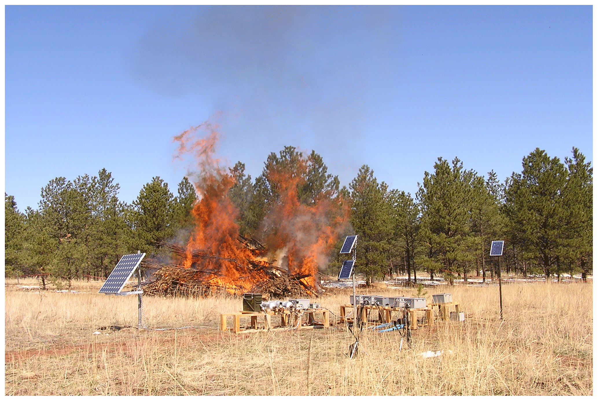
Figure 2Layout of the data system and slash pile of the MEF 26 April 2004 experimental burn about 25 min after ignition. Image credit: John M. Frank.
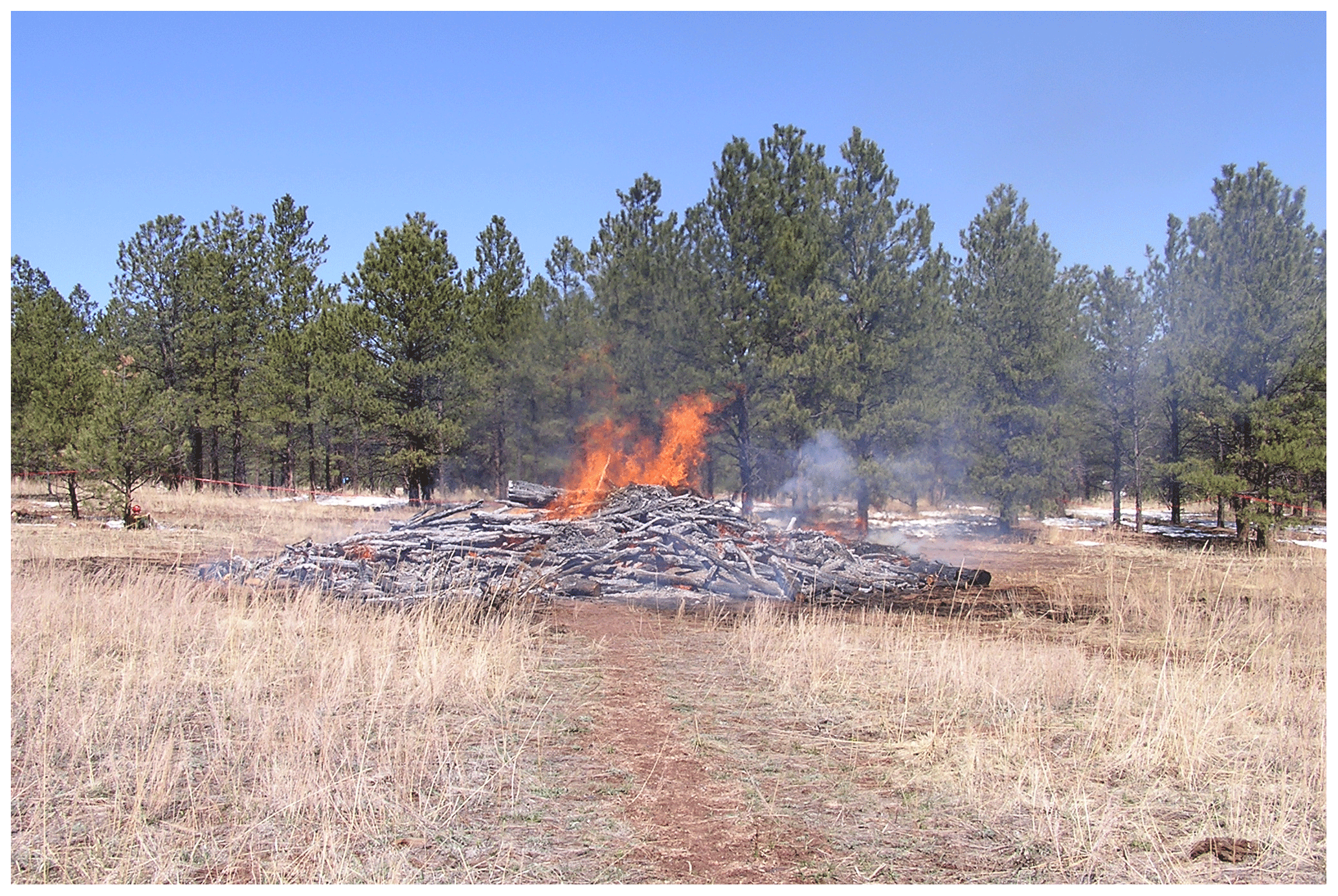
Figure 3The slash pile of the MEF 26 April 2004 experimental burn about 75 min after ignition. Image credit: John M. Frank.
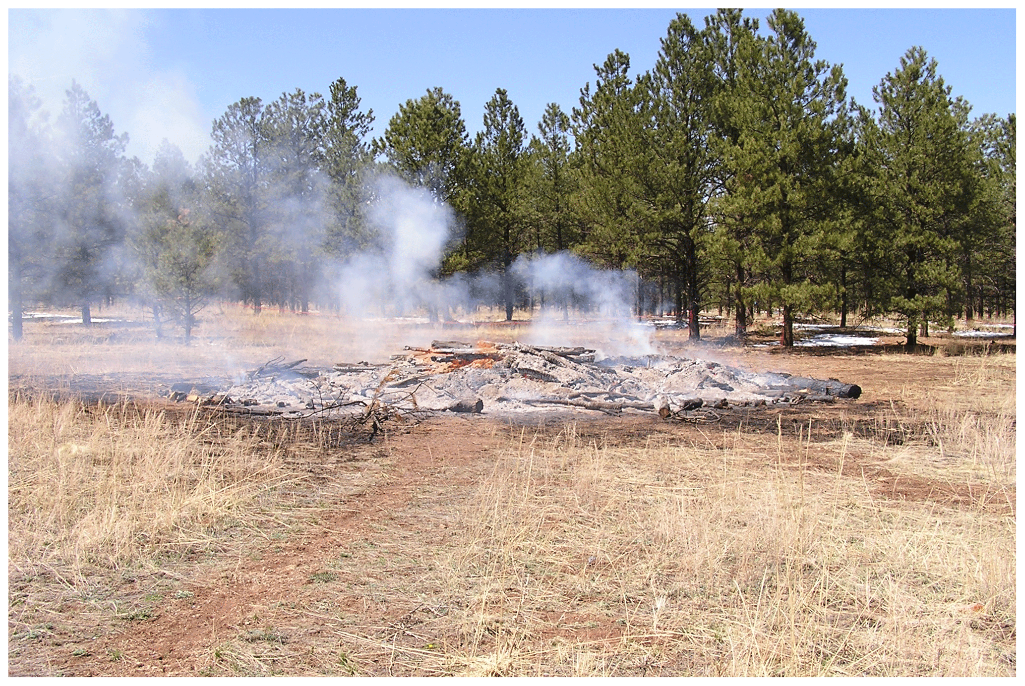
Figure 4The slash pile of the MEF 26 April 2004 experimental burn about 195 min after ignition. Image credit: John M. Frank.
3.2 The slash pile burn – description and instrumentation
The burn site instrumentation was installed in August 2003 at two control plots and two slash plots (under the center and the edge of the slash pile). Data include soil temperatures, soil moisture, soil heat flux and soil CO2 at several soil depths. All these in situ sensors and their associated connectors and cables were buried several centimeters deep and connected to data loggers (CR23X data logger; Campbell Scientific, Inc., Logan, UT, USA) via a 27 m trench that had been backfilled to protect the data communications from the heat of the fire. The slash pile (located at 3.11439∘ N, 105.10284∘ W) was mechanically constructed in March 2004 and measured about 42 m in circumference, about 6 m in height and covered an elliptically shaped area of about 130 m2. The fuel loading was estimated to be between 450 and 600 kg m−2. The burn was initiated a few minutes after 10:00 Mountain daylight time (MDT) on 26 April 2004. Figures 2–4 are a sequence of photographs taken during the first 3 h or so of the burn. Figure 2 shows the burning slash pile about 25 min after the fire was initiated and shows the deployment of the data loggers, CO2 pumps and analyzers and the supporting infrastructure. Figure 3 shows the burning slash pile about 75 min after initiation, and Fig. 4 was taken about 195 min after initiation. Note that although the soil CO2 data and the data from the edge of the pile are somewhat peripheral to this study, they are included here because they offer some important insights into some of the assumptions underlying the present model, as is discussed in a later section. Otherwise, the measured soil temperatures, soil moisture and soil heat fluxes are compared to the model's predictions and, thereby, assess and validate the model's performance.
3.2.1 Soil temperature
Soil temperatures were measured with thermocouples (Omega Engineering Inc., Norwalk, CT, USA) and sampled every 2 min during the fire and for the week following the day the fire was initiated. To insure electrical isolation, all thermocouple junctions were coated with epoxy (Omegabond 101) prior to insertion into the soil. Thermocouples were placed at the soil surface (0.00 m) and at 0.02, 0.05, 0.10, 0.15, 0.20 and 0.50 m depths. The four uppermost sensors, including the soil surface, were K-type (rated to 704 ∘C), J-type (rated to 260 ∘C), which was used at 0.15 m, and the bottom two depths were T-type (rated to 100 ∘C) sensors.
3.2.2 Soil heat flux
The soil heat fluxes were measured at three depths (0.02, 0.10 and 0.20 m) under the center of the pile with a high-temperature probe (HFT) of AlumaCore with an exterior ceramic glaze (Thermonetics Corporation, La Jolla, CA, USA). They were also sampled at the same rate and time as the soil thermocouples. These HFTs are rated to 775 ∘C and have a nominal sensitivity between 1250 and 1750 W m−2 mV−1. These HFTs were attached to a data logger by a chromel extension wire (Omega Engineering Inc.; TFCH-020; rated to 260 ∘C).
Because these HFTs are exposed to such a wide range of temperatures (potentially anywhere between about −10 and 700 ∘C), it is important to account for the effects of temperature on the sensors' thermal conductivity and calibration factors. Details concerning the calibration factor are discussed by Massman and Frank (2004) and need not be repeated here. But the details concerning the thermal conductivity of these HFTs are very relevant here and need highlighting. The thermal conductivity of these HFTs, λp (W m−1 K−1), is (where T is degrees Celsius). Knowledge of λp is important to correct for the discrepancy between the true soil heat flux, Gsoil (W m−2), and the measured soil heat flux, Gm, that results whenever λp differs from the soil's thermal conductivity, λs (Philip, 1961; Sauer et al., 2003; Tong et al., 2019). This relationship, known as the Philip correction, is given as follows:
where β is a dimensionless factor related to sensor shape (β=1.31 for the square HFTs), r is the sensor's aspect ratio, i.e., the ratio of the sensor's thickness to its horizontal length (r=0.19 for the HFTs), and . If a sensor is perfectly matched to its soil environment, then λp=λs, Gm=Gsoil, and there would be no need to correct for this discrepancy. But, in general, this is unlikely to occur very often at normal daytime or nighttime soil temperatures and so is, therefore, even less likely to occur during a fire. But this correction also requires in situ knowledge of λs, which was not (and probably could never have been) measured during this or any fire. So the model's predicted λs is used in Eq. (21). As a consequence, the model's predicted Gsoil will be evaluated against the measured heat flux, Gm, with and without the Philip correction.
3.2.3 Soil moisture and CO2
All soil moisture and CO2 data were measured at 0.05 and 0.15 m depths at both the center and edge position under the slash pile. They were both sampled every 30 min for the week during and after the burn. Soil moisture was measured using a specially designed high-temperature time domain reflectometer (TDR; Zostrich Geotechnical, Oroville, WA, USA). The design of this particular probe is fairly standard, but the material used to house the steel needles and the connectors attaching them to the coaxial (data/signal) cables had to continue operating and providing reliable data at temperatures exceeding 250 ∘C. To ensure this, external portions of the coaxial cables that were likely to be exposed to such high temperatures were wrapped in silicon tape. The calibration factor for this TDR is temperature dependent and is discussed in more detail in the Appendix of Massman et al. (2010a). As with the soil heat flux, the model's predictions will be evaluated against the TDR measurements with and without the temperature-dependent calibration factor. Soil CO2 was measured by drawing a continuous sample for approximately 0.5 min through in. (9.53 mm internal diameter) Dekabon tubing into a LI-820 (LI-COR Inc., Lincoln, NE, USA) that was housed several meters from the slash pile, as shown in Fig. 2.
4.1 Surface energy balance
Figures 5 and 6 show the details of the surface energy balance for Eq. (16), the model's upper boundary condition that includes the sensible heat and the net infrared terms. Included in Fig. 5 is the forcing function, QF(t), which shows the shape of the BFD curve. Figure 7 shows the surface energy balance for Eq. (18), which excludes the sensible heat and the net infrared terms. Comparing Figs. 6 and 7 suggests that, once tuned appropriately, either formulation of the surface energy balance will give very similar simulations of the evaporative flux, . Likewise, during the period of soil heating (i.e., when G0>0), both formulations give similar and reasonable simulations for G0. But the simplified model of the surface energy balance, Eq. (18), does not capture (and in fact cannot capture) G0 during the period when the soil is cooling (i.e., when G0<0, which starts at about 22 h in Figs. 5 and 6). Without the possibility of radiative and convective cooling of the surface, Eq. (18) does not reproduce G0<0.
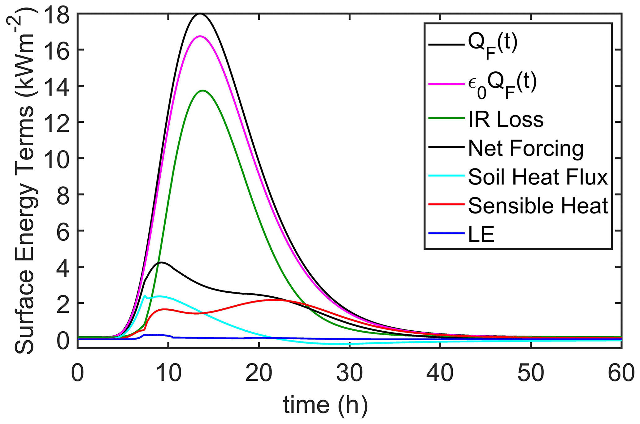
Figure 5Soil surface energy balance components for the 26 April 2004 MEF burn resulting from the full surface energy balance model (Eq. 16). The parameters for the forcing function, QF(t) or Eq. (15), are Qin=120 W m−2, QFmax=18 kW m−2, tm=13.5 h and td=35 h. The net forcing is defined as the difference between the radiative terms, i.e., , which, from Eq. (16), is equal to the sum of the three nonradiative terms, i.e., . Figure 6 is an magnified version of the net forcing and these three energy components.
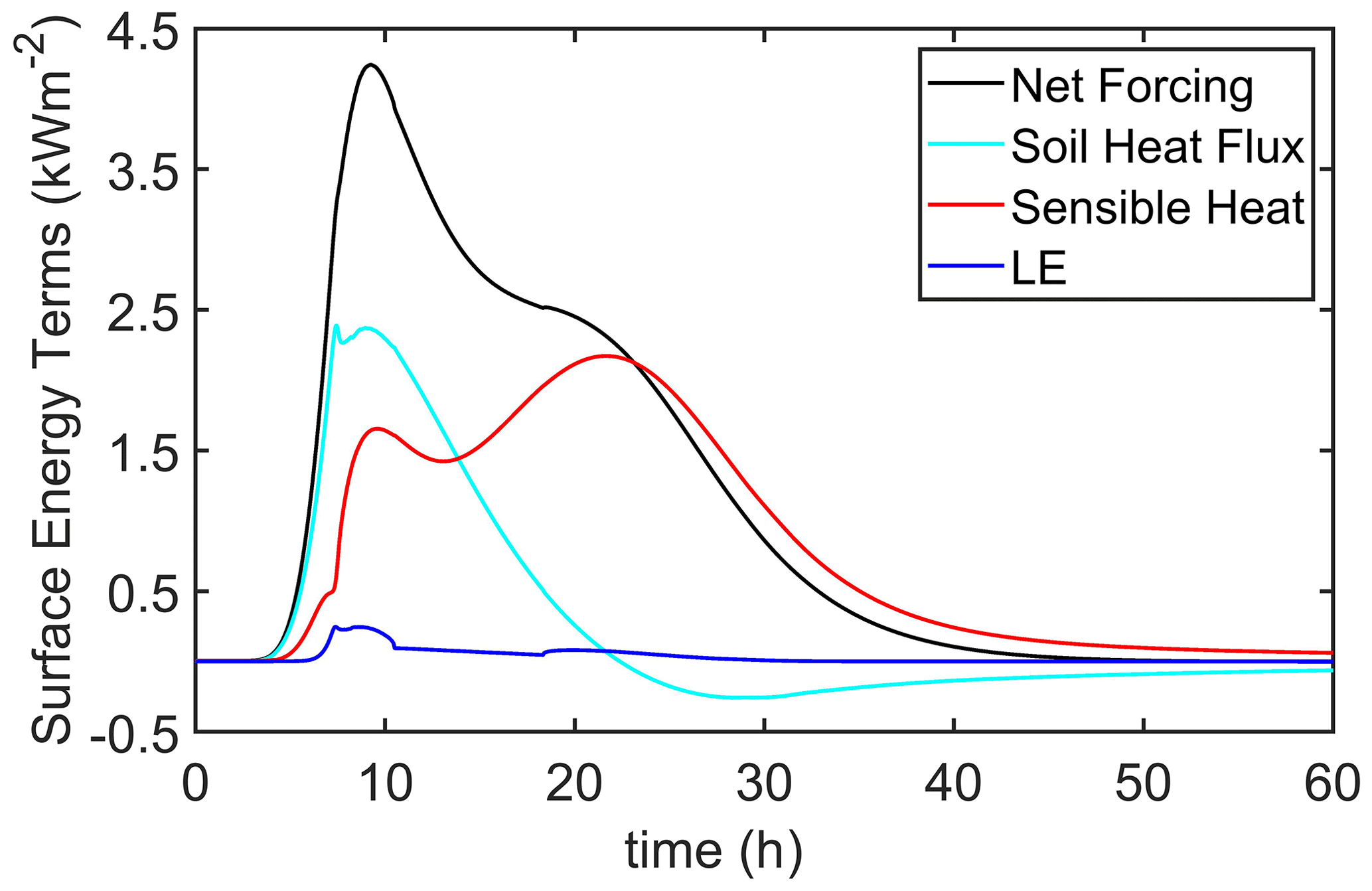
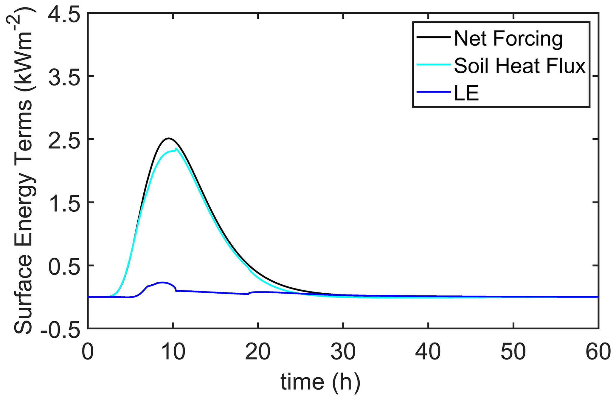
Figure 7Soil surface energy balance components for the 26 April 2004 MEF burn resulting from the simplified surface energy balance model (Eq. 18). The parameters for the forcing function, QF(t) or Eq. (15), are Qin=0 W m−2, QFmax=2.7 kW m−2, tm=9.5 h and td=27.5 h. Here the net forcing is the sum because the surface sensible heat flux is not included as part the simplified surface energy balance.
Another important aspect about the surface energy balance that Eq. (18) does not capture as well as Eq. (16) is the time lag between the maximum in soil heat flux and the maximum in soil temperature. At 0.02 m depth, the observed time lag is about 5 h. Predictions of the time lag with the full surface energy balance, Eq. (16), agree almost exactly with the observed time lag. But the simplified model predicts a time lag of about 4.6 h. This difference in the time lags is not the result of the different choices of tm, td or QFmax between the two models of the surface energy balance. Instead, Eq. (18) inherently constrains the soil heat flux more strongly than Eq. (16).
These apparent limitations of the simplified surface energy balance, Eq. (18), do not lessen the argument that it may be appropriate for some slash pile burns or any time that burning material is in direct contact with the soil, and the concomitant soil heating is overwhelmingly conductive. Instead, these present comparisons suggest that a hybrid of Eqs. (18) and (16) may be more appropriate. Such a hybrid would employ Eq. (18) in the early part of the burn (before significant loss of mass from the slash pile due to combustion) and Eq. (16) later after the fire intensity has peaked (i.e., sometime after td), when the soil surface or possibly an ash surface is more exposed to the ambient environment. The time course of the experimental burn, shown in Figs. 2–4, is consistent with a hybrid formulation of the boundary forcing. Nonetheless, it is beyond the intent of the present paper to explore this concept any further.
Other than these two discrepancies, the two forms of the surface energy balance give very similar simulations for soil temperature, moisture and other model variables. Nevertheless, because the full surface energy balance provides the more physically realistic simulation, it will be used throughout the remainder of this study.
4.2 Soil temperature
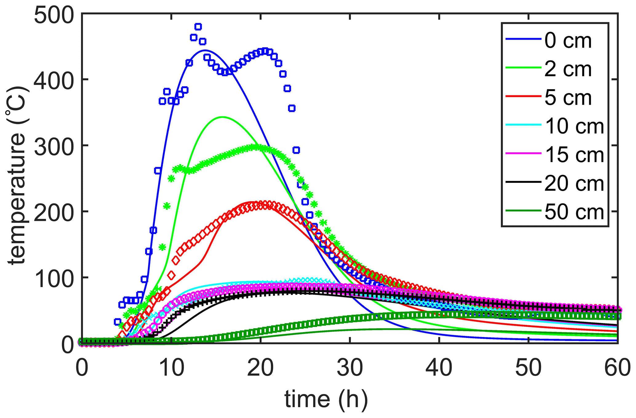
The principal aim of this model is to simulate reasonable and realistic soil temperatures during fires. The comparison between modeled and observed soil temperatures, shown in Fig. 8, suggests that the HMV model with the current set of tuned parameters is reasonably good at this task. Nonetheless, a careful examination of the features of this Fig. 8 shows some slight discrepancies in the model's performance. (1) The model does not capture the early temperature rise beginning at about 4 h, (2) nor does it capture the secondary maximum temperature at about 20 h. (3) It appears to overestimate the maximum 2 cm soil temperatures (at about 21 h), and (4) the soil appears to cool off faster than observed (most obvious after about 28 h). Discrepancies (1) and (2) are not unexpected because it is impossible for a simple forcing function like the BFD curve and Eq. (15) to produce an exact or even a near-exact simulation of the observed temperature dynamics during a fire. Any real physical surface forcing will always be far more (dynamically) complex than the BFD curve, and it could not be easily generalized from one fire to the next. The (relatively significant) overestimation by nearly 60 ∘C of the 2 cm soil temperatures is not fully understood, but it may be a consequence of a mismeasurement of the installation depth of the soil temperature sensors and/or poor contact with the soil, meaning that the soil air in contact with the temperature sensor would be acting as an insulator relative to the heat conducting soil particles in contact with the sensor. It is also possible that λs possess greater vertical structure than is included in the model. This could easily be the case for MEF soils because the present model of λs neither includes the observed vertical structure in soil bulk density nor its relationship to the vertical structure of the soil's thermal conductivity (Massman et al., 2008). Finally, the issue involving the difference between the observed and modeled rates of cooling, discrepancy (4), seems to be characteristic of all model simulations and not just the simulation shown in Fig. 8. Some of this is undoubtedly related to the simple shape of the BFD curve (forcing function) and the constraints it imposes on the upper boundary conditions. Another likely contributing factor to discrepancy (4), and the other three issues, is the ash layer that formed during the fire. A month after the fire, the ash layer measured between 0.5 and 8 cm deep within the burn area and was about 2 cm deep over the area where the sensors were buried. Because the ash layer would have insulated the soil surface, it would have acted to slow the rate of cooling as the fire died out.
4.3 Soil heat flux
Comparisons between measured and modeled heat fluxes, shown in Fig. 9, are an independent check of the mathematical structure and tuning parameters of the surface forcing function, QF(t). For this study, QF(t) was tuned primarily for soil temperatures and secondarily for soil heat flux. Figure 9 compares the observed heat fluxes (blue color-filled area and symbols) to the modeled heat fluxes (solid lines). The upper boundary of the (2 cm) blue color-filled region is the heat flux measured by the heat flux plate without the Philip correction. The lower boundary of this region is the measured heat flux with the Philip correction, indicating that, for this experiment, the Philip correction reduced the amplitude of the uncorrected flux. The Philip correction is not shown for the two lower heat flux measurements (symbols) because it made virtually no change in the uncorrected fluxes. In general, the model does appear to capture many features of the observations. Of particular interest is the fact that the amplitude of the modeled heat flux more closely resembles the Philip-corrected heat flux, providing confidence in both the model's performance and the quality of the soil heat flux data. On the other hand, the modeled heat flux peaks several hours before the measured heat fluxes do. Without significantly increasing the complexity of the forcing function and the concomitant tuning effort, it is (at best) unlikely (if possible at all) to improve much on the model's ability to reproduce the observed temperature and heat flux data for this burn.

Figure 9Soil heat flux during the 26 April 2004 MEF burn, with modeled (solid lines) and observed (blue color-filled area and red and black symbols) measurements. The upper boundary of the (2 cm) blue color-filled region is the heat flux measured by the heat flux plate without the Philip correction (Philip, 1961). The lower boundary of this region is the measured heat flux after applying the Philip correction. The Philip correction is not shown for the two lower heat flux measurements because it made virtually no difference to these measurements.
4.4 Soil moisture
The modeled soil moisture is shown as a function of time in both Figs. 10 and 11 for the same depths (and color coding) as shown for temperature in Fig. 8. Included in each figure is the soil moisture measured at 5 cm (red) and 15 cm (magenta) depths, but Fig. 10 includes the temperature-corrected calibration of the soil moisture probe, whereas Fig. 11 does not. The red (5 cm) stars are interpolated values, which replace values that were flagged by the noise filter as questionable. Nonetheless, confidence in the fidelity of these interpolated values is high. But confidence in the magenta (15 cm) stars (also interpolated) is less. Rather interestingly, the modeled 5 cm soil moisture agrees better with temperature-corrected soil moisture, whereas, at 15 cm, the model resembles the uncorrected 15 cm soil moisture. Consequently, both figures are included here to show the importance of the temperature effects on the high-temperature TDR and to provide an estimate of the uncertainty inherent in these soil moisture measurements.

Figure 10Volumetric soil moisture, after temperature correction to the TDR probe (Massman et al., 2010a, Appendix A), during the 26 April 2004 MEF burn, with modeled (solid lines) and observed (symbols) measurements. The color coding for depth is the same as that in Fig. 8, but observations of soil moisture are taken only at two depths, i.e., 5 cm (red) and 15 cm (magenta). The red stars are interpolated values and appear to be fairly trustworthy. The magenta stars are less trustworthy because the performance of the 15 cm TDR during the early part of the burn was not completely satisfactory.
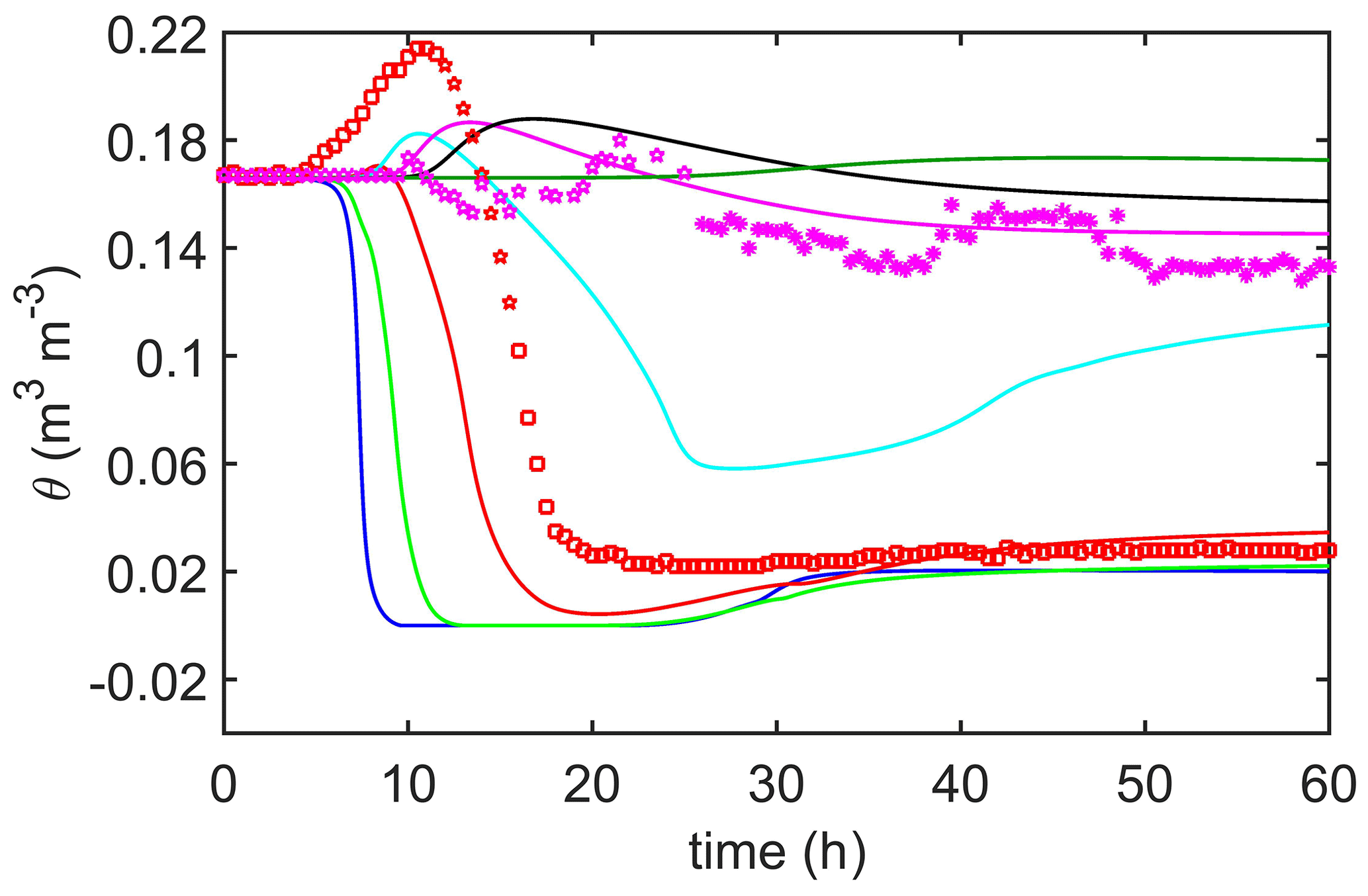
Figure 11Volumetric soil moisture, without temperature correction to the TDR (Massman et al., 2010a, Appendix A) during the 26 April 2004 MEF burn, with modeled (solid lines) and observed (symbols) measurements. The color coding for depth is the same as that in Fig. 8, but observations of soil moisture are taken only at two depths, i.e., 5 cm (red) and 15 cm (magenta). The red stars are interpolated values and appear to be fairly trustworthy. The magenta stars are less trustworthy because the performance of the 15 cm TDR during the early part of the burn was not completely satisfactory.
Figure 12 shows the observed (temperature-corrected) soil moisture versus the observed temperature along with the model's solutions of θ vs. T (or the model's θ−T trajectory). Here the model predicts that, for depths less of than 5 cm, the soil moisture begins to evaporate (decrease) between 50 and 90 ∘C, and that these initial evaporative temperatures increase deeper into the soil. Nonetheless, the model suggests that the soil does not dry out completely until temperatures have reached about 200 ∘C. The observations at 5 cm show a similar pattern to the model, except these observations suggest that the initial evaporation stage proceeds more slowly, and that overall evaporation occurs at a higher temperature. The same observation was made by Massman (2012) and Massman (2015) regarding the laboratory data of Campbell et al. (1995). Several test simulations were performed to see if the model could be made to better emulate the observed θ−T trajectory, including different formulations and parameter values for KR; different parameter values for the forcing function, QF(t), and the simplified surface energy boundary condition, Eq. (18); and different WRCs, variations in the parameters of the source term, Sv, and removing the enhancement factor from the vapor diffusivity, Dve and Eq. (4). Only changes in Sv and Dve made any significant positive difference to the model's θ−T trajectory. Changes in either of these model factors can strongly influence the amount of vapor within the soil pores, which in turn influences the soil moisture dynamics. This should not be too surprising in the case of Sv because Sv is formulated within the present model as a balance between the physical processes that govern evaporation and condensation to and from soil surfaces, and, therefore, influences the balance between soil moisture and soil vapor. In the case of reducing the enhancement factor (i.e., assigning it a value of one), the resulting decrease in vapor diffusivity causes the vapor within the soil pores to increase such that it feeds back to soil moisture via the condensation term of Sv (proportional to ρv; Eq. 9), again influencing the balance between θ and ρv. This exploration of the modeled and observed θ−T trajectory has yielded some insights into what maintains the long evaporative tail (where some soil moisture persists well past the boiling point of water), an issue that was less understood in Massman (2012) and Massman (2015).
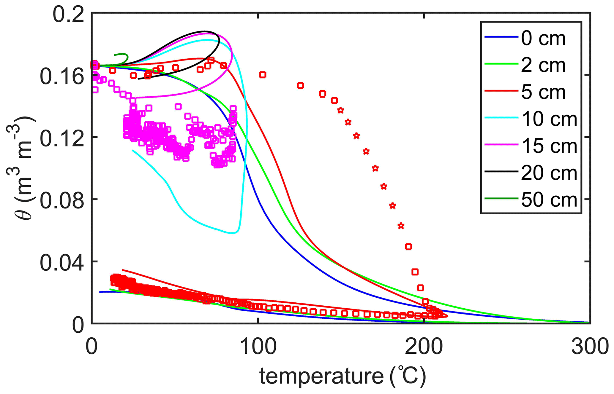
Figure 12Modeled and observed θ−T trajectory. Observed data are denoted with symbols and modeling results are solid lines. The observed volumetric soil moisture has been temperature corrected.
Taken in total, the model's simulation of soil moisture agrees with the observations fairly well. It is, of course, possible to improve on the model's fidelity to the observations by adjusting KR or changing the heating rates or duration and magnitude, QF(t), and, most importantly, by changing the values of the parameters of Sv and Dve that influence soil vapor, ρv, but usually this comes at some expense with respect to the model's fidelity to the measured soil temperatures. The same issue was noted in Massman (2012) and Massman (2015). Thus, the present choice of model parameters is a compromise between two or three somewhat conflicting goals, i.e., fidelity to the soil's thermal response to heating by fire and the soil's moisture and vapor response.
4.5 Dynamic feedbacks
Fire changes soil, and the more intense the fire and the greater amount of soil heating, the greater the changes in the soil will be. Although this statement should be self-evident, it is probably more precise to say that changes in the soil result from the integrated effects of the surface heat flux (delivered to the soil), the area of soil in contact with or influenced by the fire and the duration of the fire. That is, the probability of the change in soil due to fire is . This more precise approach clearly suggests that changes in the soil are more likely to occur during spatially stationary fires (e.g., slash pile burns or relatively low-intensity but long-duration biomass burning) than during a fast-moving, dynamic fire (such as a grassland fire or a low shrubland fire or even an extremely high-intensity crown fire).
Examples of some of the changes that are relevant to the present study include (a) changes in the soil bulk density (Gregory Butters, personal communication, 2009; Kojima et al., 2018), which will alter the WRC (Fig. 1) and hydraulic properties (Tian et al., 2018), (b) changes in the thermal conductivity of the soil (Massman et al., 2008; Kojima et al., 2018) and the volumetric specific heat (Gregory Butters, personal communication, 2009), (c) changes in the heat and vapor fluxes resulting from (a) and (b) (Kojima et al., 2018), and (d) changes in the soil's specific surface area, Awa, and particle surface potentials, which result when the fire induces water repellency in soils (Chen et al., 2018). None of the physical/chemical processes causing these phenomena are included in any extant model of soil heating during fires. Part of the difficulty is that these dynamic feedbacks occur during fires; consequently, they influence soil heating and moisture transport in situ during the fire. To give some idea of how these dynamic feedbacks may influence the soil heat and moisture transport, this section details the results of a model simulation based on observed or inferred changes in the bulk density and key thermophysical parameters.
The following model parameters were changed for this sensitivity analysis to feedbacks: soil bulk density increases from 1.30 to 1.46 Mg m−3 (a 12 % increase, as per Fig. 1); simultaneously, the thermal conductivity of the mineral fraction, λm0, increases from 4.42 to 8 Wm K−1; the de Vries shape factor, ga, decreased from 0.123 to 0.06; the Campbell et al. (1994) parameter qw0 (which determines when the water content starts to influence the soil's thermal conductivity) decreased from 0.03 to 0.02; the soil's volumetric specific heat increases by 10 % (in accordance with the observations made by Gregory Butters, personal communication, 2009); the overall soil thermal conductivity, λs, increases by 15 %; and, finally, the source term coefficient, S*, decreases from 0.1 to 0.08 (specifically chosen to be a 20 % decrease). This increase in bulk density yields a concomitant decrease in soil porosity, η, which is simply carried over in a purely linear fashion to the soil thermal conductivity, the WRC, the hydraulic conductivity function and the source term, Sv. On its own this decrease in η yields an increase in Sv. But under extreme drying it is more reasonable to expect Awa (and Sv) to decrease (Chen et al., 2018); so, to compensate, S* is reduced when η is reduced. It very natural to expect the soil's thermal conductivity to increase with the increase in bulk density, but the present model of thermal conductivity does not explicitly include any dependency on ρb. So λs is increased by 15 % to accord with the increase predicted by the model developed by Johansen (1975). Changes in ga and qw0 are intended to capture the observation (Massman et al., 2008) that the fire decreased the sensitivity of the soil's thermal conductivity, λs, to soil moisture, (i.e., decreased as a result of the fire) and increased λs when the soil was dry (θ<0.08). Decreasing ga and qw0 was the best way to capture this pair of observations. In addition, a decrease in ga was also observed by Smits et al. (2016) for fire-affected soils. The conductivity of the mineral fraction, λm, was increased to capture the creation of thin, but highly conductive, coatings of mineral oxides (MnO2 in particular) on the soil particle surfaces during the MEF experimental burn (Massman et al., 2010b; Nobles et al., 2010). Such thin coatings are synthetically created for routine application to nanotechnologies (e.g., O'Brian et al., 2013).
The base case model simulation (Figs. 8–12) and the feedback simulation are compared in Figs. 13–15. The upper boundaries of the color-filled areas in Fig. 13 (temperature) and Fig. 14 (heat flux) correspond to the feedback simulation, whereas the lower boundary in Fig. 15 (soil volumetric moisture) is associated with the feedback simulation. These comparisons demonstrate that the feedbacks overwhelmingly act to increase the soil temperatures and heat fluxes throughout the soil and to significantly increase evaporation and evaporative losses of soil moisture (at least within the upper few centimeters of soil). However, the change in bulk density alone is responsible for about half of the differences shown in these figures. Overall, though, these last three figures indicate that these dynamic feedbacks are potentially quite significant to the magnitude and depth of the soil heating. Or, paraphrasing somewhat, during a fire, soil temperatures are not a direct linear response to the surface forcing function; rather, at any given moment, the soil heating feeds back (nonlinearly) upon itself, creating conditions that allow the heat to penetrate more deeply into the soil and allowing the soil temperatures to exceed what they would have been without the feedbacks.
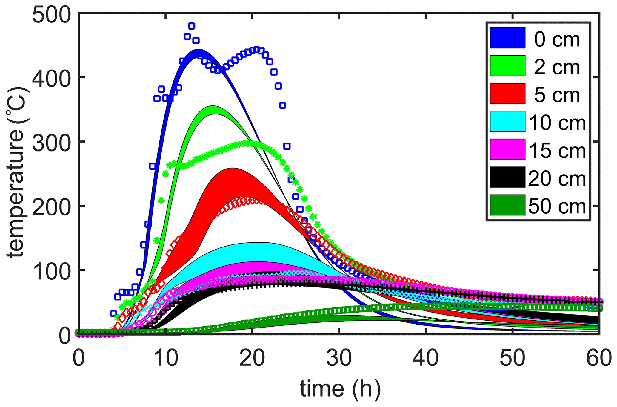
Figure 13Potential impacts of dynamic feedbacks on the soil temperatures during the 26 April 2004 MEF burn. Observed data are denoted with symbols and modeling results are solid filled areas. The lower boundary of the solid filled areas corresponds to the base case simulation and the upper boundary to the feedback simulation.
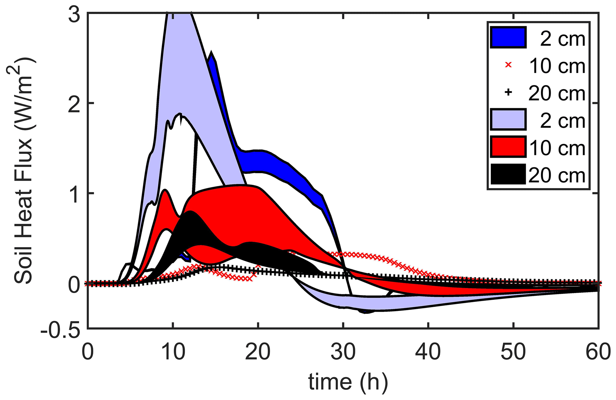
Figure 14Potential impacts of dynamic feedbacks on the soil heat flux during the 26 April 2004 MEF burn. The observed data are shown as the (2 cm) darker blue color-filled area and red and black symbols. The upper boundary of the observed heat flux includes the Philip correction, whereas the lower boundary of this region is the measured heat flux after applying the Philip correction. The Philip correction is not shown for the two lower heat flux measurements because it made virtually no difference to these measurements. The upper boundary of the light blue, red and black color-filled areas corresponds to the feedback simulation and the lower boundary to the base case simulation.
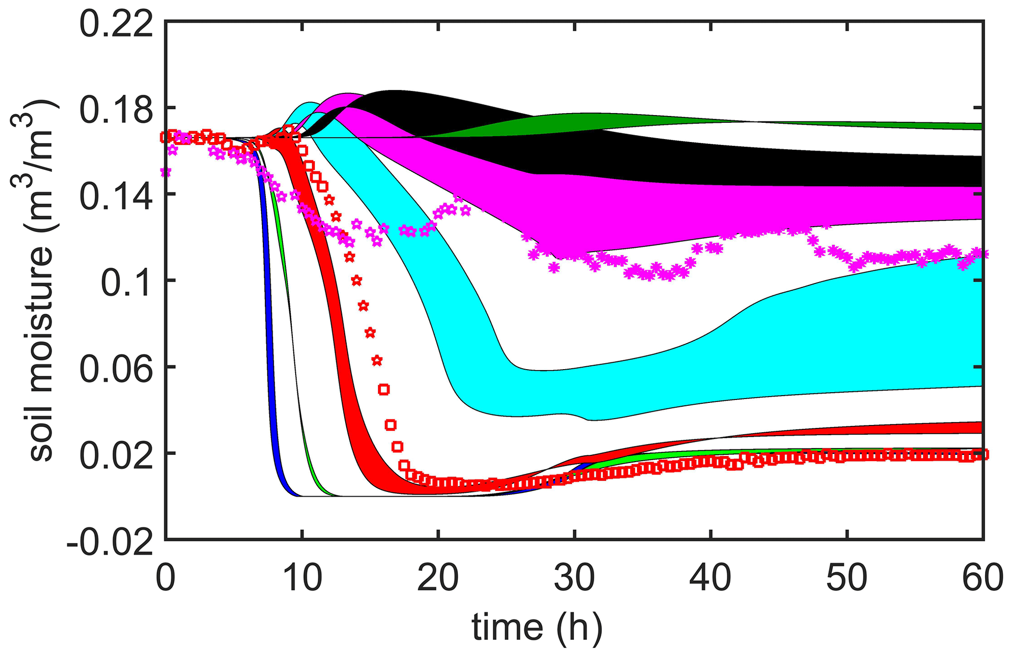
Figure 15Potential impacts of dynamic feedbacks on the volumetric soil moisture during the 26 April 2004 MEF burn. Observed data, which has been temperature corrected, are denoted with symbols, and modeling results are solid filled areas. The upper boundary of the solid filled areas corresponds to the base case simulation. The lower boundary corresponds to the feedback simulation.
Although the HMV model gives reasonably realistic simulations of soil temperatures and moisture during fires, there are several enhancements that may further improve its performance, and these should be useful to consider for future studies of the soil's response to heating during fires.
- a.
Dynamic feedbacks and soil thermal conductivity – a better physical understanding of the dynamical processes that govern how extreme heating during fires changes ρb and the development of a model of λs that captures this dynamic is needed. Also, there needs to be a better formulation of how soil structure influences ga and λs and how soil structure changes during a fire. This issue of improving model parameterizations of λs is more complex than just including ρb because the observed increase in λs for a dry soil was 200 %–300 % (Massman et al., 2008), which far exceeds the 15 %–17 % predicted by the model of Johansen (1975).
- b.
Mass transport – the present version of the HMV model assumes an advective transport of water vapor induced by the rapid volatilization of the soil moisture, i.e., uvl and Eq. (5). But most formulations of advective transport in soils are based on Darcy's law. For application to fire, uvl from Darcy's law would result from the rapidly evolving vapor pressure and temperature gradients. Additionally, it would be worthwhile to include the dry air density, ρd, as a separate model variable. Certainly, in any real fire, the temperature and pressure of the dry air within the soil pore spaces would respond dynamically to heating. But including ρd as a dynamic variable should yield a more physically realistic simulation of the diffusional and advective transport of water vapor during the fire. The results of Zeng et al. (2011) for less extreme conditions support this notion. Finally, given the potential for extreme gradients in soil water potential and temperature during fires, it may also be worthwhile to include the heat transported by the movement of water (e.g., Stallman, 1965; Pasquale et al., 2014) in Eq. (1). This energy transport term has often been included when modeling the daily cycle of energy flow through soils. Because some fires, especially slash pile burns, can continue for a week or more, it seems appropriate to investigate the influence that this type of energy transport could have on model solutions.
- c.
The 2D and 3D effects – there are (at least) two physical processes that cannot be fully represented in a 1D model, i.e., (i) horizontal heat flux (Ghor) and (ii) possible advective currents (here characterized by an advective velocity uadv) induced in the soil shortly after the pile is ignited (Massman et al., 2010a, b; Nobles et al., 2010). (i) In an earlier section, mention was made of the second installation of soil sensors at the edge of the pile. With these data, used in conjunction with the soil temperature data at the center of the pile, it is possible to obtain a crude estimate of the horizontal temperature gradient. Then, assuming that horizontal and vertical thermal conductivities (at the same depth) are about the same in magnitude, it is possible to show that Ghor during the fire is approximately 10 % of the vertical soil heat flux. This estimate of Ghor was confirmed with data taken during another experimental burn, performed in the fall of 2004, in which the 20 or so temperature sensors were placed in a horizontal array that allowed about 20 different horizontal gradients to be compared with about the same number of vertical gradients. This is relevant to the present study because it may help explain some of the divergence between modeled and observed soil temperatures and (vertical) heat fluxes, and it further underscores the nature of the challenges and empiricism inherent in the modeling of soil heating during fires. (ii) Far more important for any further studies is the possibility of a fire-induced uadv because it appears to be inherently 2D or 3D in nature and it appears to carry combustion products into the soil (Massman et al., 2010b, Fig. 4). Such an advective current is hypothesized to have caused the extremely rapid 20-fold increase in soil CO2 which was observed to have occurred within the first 30 min of the Manitou burn being modeled here (Massman et al., 2010a). Consequently, any combustion-produced water vapor will also be transported. If this is the case, it would likely overwhelm uvl and contradict assumptions made about evaporation at the soil surface and the transport of soil water vapor during (at least) some portion of the burn. It may be possible to just impose uadv in a 1D model like the HMV model, but such an adjustment should probably be guided by observational studies and experiments designed to establish the existence, nature and dynamics of uadv.
This study describes the continuing development, improvement and validation of the HMV model, which is a nonequilibrium model of the coupled transport of heat, moisture and water vapor in soils during surface fires. The purpose of the research supporting this study is to provide a tool to aid in the management (and reduction, if possible) of the physical and ecological affects of fire on soils. In fact, a version of the HMV model is currently available to land managers through the USDA Forest Service's First Order Fire Effects Model (FOFEM) version 6.7 (USDA Forest Service, 2020). Key improvements to the model, which noticeably improved its stability and performance, include more physically realistic parameterizations of the nonequilibrium vapor source term, Sv, and soil thermal conductivity, λs. Integral to the validation of this model are the development of a general surface heating (forcing) function and discussions of the complexities and difficulties regarding formulating the surface (or upper) boundary condition. The model is validated using in situ measurements of soil temperatures, heat flux and soil moisture obtained during a 2004 experimental burn carried out at MEF (in the central Rocky Mountains of Colorado). Despite any possible ambiguities in the calibration of the soil moisture and heat flux sensors, and given the simplicity of the modeled forcing function and the complexities of the true forcing that can be inferred from the dynamics of the soil data, the model's ability to reproduce the observations is at least reasonable and maybe even surprisingly good. But, as with Massman (2012) and Massman (2015), tuning the model parameters requires navigating the somewhat divergent goals of achieving a best fit to either the soil temperature observations or soil moisture observations. Absent to the model are important fire-induced feedbacks, in particular in situ changes in the soil's thermal and hydraulic properties that are inevitable when the fire (as is often observed) causes the soil's bulk density to increase. This important dynamic was investigated with a model sensitivity analysis by making logical and credible changes to the (appropriate) model parameters. The net affect of this feedback is that the heat pulse will propagate much deeper into the soil than it would have otherwise, pointing to the need for further observational and modeling studies of this phenomenon. This study closes by highlighting other areas of research needed to improve our understanding of and ability to model the physical processes that occur in soils during fires, including issues involving the transport of both soil moisture and soil vapor during fires, the potentially very significant 2D or 3D advective flows in soils induced by fires and the possibility of 2D or 3D heat flow.
A1 Mass gradient diffusional flux ()
De Vries (1958) defines the soil's apparent thermal conductivity, λs,app, as the medium's thermal conductivity, “including the effect of the vapor distillation due to temperature gradients”. But, in a modeling context, the use of λs,app has to be treated with some care because it is inappropriate to externally introduce λs,app into the equation for conservation of energy (employed universally as part of any model of heat and moisture flow in soils). This appendix develops both an equilibrium and a nonequilibrium model for λs,app to illuminate its thermodynamic origins and to clarify its proper role in the modeling of soil heat and moisture flow in soils. Before proceeding, note that all terms relating to advective vapor flow (i.e., uvl) and liquid water flow (i.e., Kn, KH and Vθ,surf) can be ignored because they are superfluous for purposes of this appendix.
The basic conservation equations employed in this study are Eqs. (6), (7) and (4). But there is a valid alternative expression for Eq. (6), which results from the combination of the conservation of enthalpy, Eq. (1), with the conservation of water vapor, Eq. (4), and the equilibrium assumption (), and is expressed as follows:
which, after some simple mathematical manipulation, can also be written as follows:
where the last term on the right-hand side of this equation accounts for moving inside the gradient operator . As discussed in the main text, is modeled by the Kelvin equation, and , so that can be expanded in terms of , and in terms of and . The following shows . (Note that can be found by substituting t for z).
where Δsat (kg m−3 K−1) is the slope of the saturation vapor curve, , and is for temperatures between about 5 and 60 ∘C. Furthermore, unless the soil is extremely dry (, implying that the second term that multiplies the temperature gradient of Eq. (A3) can be ignored relative to the first term for most applications. Otherwise, for an extremely dry soil, . Henceforth, . In addition, it is always true that , which means that the rightmost term in Eq. (A3) can also be ignored. Therefore, Eq. (A3) is now as follows:
Substituting Eq. (A4) into Eq. (A2) yields the following:
where the term has been dropped from Eq. (A2) because (although it is a bit tedious to show). Equation (A5) yields the following identification for λs,app:
where the term describing the effect of the vapor distillation due to temperature gradients on the soil's thermal conductivity is (identified in Eq. (A6) as λs,dis). This expression for λs,app is often used as the justification for including the effects of vapor transfer on λs, i.e., the substitution of λs,app for λs in the equation of the conservation of enthalpy in soils (e.g., Hillel, 2004, Eq. (12.24), p. 226; Campbell et al., 1995; Smits et al., 2011; Massman, 2015). But, as this Appendix shows, in a modeling context, this substitution is usually unnecessary (and inappropriate) because these vapor transfer effects are already either directly or indirectly embedded in the equation for conservation of enthalpy.
Next is the introduction of the equilibrium assumption, Eq. (A4), into Eq. (7). This yields the following:
or to a very good approximation (which follows from Eq. (A7) because ), as follows:
Equations (A5) and (A8) now form an equilibrium model with two independent predictive variables (T and θ or ψ) that describe the coupled heat and moisture flow in soils. This particular model clearly results in and is completely consistent with the soil's apparent thermal conductivity, λs,app. On the other hand, there is an equally valid model of this coupled dual-variable model for which λs,app is not only unnecessary, but it would, in fact, be an error to invoke its use with the model.
This other coupled heat and moisture flow model combines the conservation of mass for water (liquid and vapor; Eq. (A8) above) with the simplified version of the conservation of energy equation, Eq. (6), as discussed in the development of the nonequilibrium model. This simplified equation is as follows:
It is important to reiterate that the paired Eqs. (A8) and (A5) are as valid a basis for describing coupled heat and moisture flow in soils, as are the paired Eqs. (A8) and (A9), although Eqs. (A8) and (A9) are much more extensively used. But the conservation of energy equation, as expressed with Eq. (A9), does not explicitly include the effect of the vapor distillation due to temperature gradients (λs,dis), whereas Eq. (A5) does. Instead, the effects of the distillation of water vapor are implicit in Eq. (A9) because they are included in (via Eq. A8). Therefore, to substitute λs,app for λs in Eq. (A9), or any θ-based variant of Eq. (A9) (as opposed to a ρv-based variant like Eq. A5) on the assumption that λs should explicitly include the effects of water distillation, is incorrect because to do so is to double count the effects of λs,dis on soil thermal energy transport. This double counting is even more obvious (using the same argument that λs should include the λs,dis term) when λs,app is substituted for λs in Eq. (A5), which already explicitly includes λs,dis.
The nonequilibrium form of λs,app follows from the same general methodology as the equilibrium form from Eq. (A5) does. First, combining Eqs. (1) and (4) and then simplifying yields the following:
Next, employing the ideal gas law for ρv, i.e., , yields the following:
Finally, introducing Eq. (A11) into Eq. (A10) yields the following:
where the nonequilibrium form of λs,dis is now . For practical applications, this is obviously not as convenient or as useful as the equilibrium form because λs,dis is now a function of ρv, which, for most experimental settings in soils, is difficult (if not impossible) to measure directly. Nonetheless, for the purposes of this Appendix, it suffices to show that a nonequilibrium model of λs,dis can be defined, and that, in a modeling context, it is just as unnecessary and inappropriate to use – as is the better known equilibrium version of λs,dis.
To summarize and conclude, the conservation of enthalpy (Eq. 1, or one of its many derivatives, e.g., Eqs. 6, A5 and A9), is fundamental to all models of heat and moisture flow in soils. All forms of this conservation law also explicitly include the effects of the phase change of water through the vapor source term, . Therefore, all effects associated with the distillation of water are a result of Sv. This is true whether discussing either an equilibrium or nonequilibrium model. Imposing or assuming liquid/vapor equilibrium or nonequilibrium has mathematical consequences with regard to how ρv and Sv are parameterized and can also have indirect influence on the soil's intrinsic thermal conductivity (λs) because λs is a function of several variables, among which there are soil volumetric water content and soil vapor density, i.e., (de Vries, 1963; Campbell et al., 1994; Tian et al., 2016). But, within a modeling context, there is no justification for substituting the apparent thermal conductivity, λs,app, for the soil's intrinsic thermal conductivity, λs, in the equation of conservation of enthalpy (Eq. 1). To do so violates the conservation of enthalpy by effectively double counting λs,dis.
A2 Mass mixing ratio diffusional flux ()
The discussion in this section of the appendix complements the discussion of λapp and λs,dis in Sect. A1 above. It does not change the final outcome or conclusions reached in Sect. A1. Section A2 is included here only to further refine λs,dis. Furthermore, results of this section are limited to relatively moist soils, for which λs,dis is of greatest interest and significance.
The discussion in Sect. A1 above develops λs,app more or less along the traditional lines, using the mass gradient form of the diffusional flux, . But the diffusional flux is also represented (and sometimes more appropriately represented) in terms of the gradient of the mass mixing ratio, i.e., , where ρa (kg m−3) is the total (dry air and vapor) soil gas density and χv (kg kg−1) = . This section of the Appendix shows that, for a relatively moist soil (i.e., aw≈1 and ), λs,dis developed in Sect. A1 above differs between +2.5 % (for T≈5 ∘C) and −4.5 % (for temperatures T≈60 ∘C) from that given in Eq. (A6). All that this requires is a demonstration of how generalizes Eq. (A4).
From the identity , where ρd (kg m−3) is the soil dry air density, it follows that:
Next, assuming that ρd is an ideal gas, it follows that:
Because the pressure gradient term, , is not relevant for the present purposes (and it is unlikely to contribute much to anyway), it can be dropped from Eq. (A14). This yields the following:
which, after combining with Eq. (A4) and some further simplification, yields the following:
from which it follows that:
This last expression indicates that there are two (moderately) compensating terms to λs,dis that do not occur in the diffusional mass flux form for the apparent thermal conductivity. These are () instead of 1 and instead of . At about 5 ∘C, χv≈0.005 and , whereas, at 60 ∘C, χv≈0.10 and . These results imply that, at 5 ∘C, Eq. (A17) will yield a value for λs,dis that is about 2.5 % higher than and that, near 60 ∘C, Eq. (A17) yields a value for λs,dis that is about 4.5 % lower. Unless a correction between +2 % and −4.5 % is important for estimating λs,dis, it seems that the mass mixing ratio formulation for the diffusional mass flux (Eq. A17) adds very little value to the original formulation (Eq. A6).
The MATLAB (version 2017b) model computer code described in this study, all soil heating data, and the computer code used for graphics are publicly available via the Fort Collins, CO, Forest Service Research Data Archive at https://doi.org/10.2737/RDS-2020-0077 (last access: February 2021; Massman, 2021). All archived materials are also freely available from the author upon request.
The author declares that he has no conflict of interest.
The author would like to thank Michael D. Novak for his continued interest in this research and for many discussions on various aspects of this work. I would also like to thank Gerard Kluitenberg for sharing his time for discussions on all aspects of soil physics relevant to the research discussed in this paper. Finally, I would like to thank Curtis Monger (USDA Natural Resources Conservation Service (NRCS) National Soil Survey Center) for his help with identifying the FAO UN (2014) classification of the Manitou Experimental Forest soil.
This paper was edited by Nunzio Romano and reviewed by Yijian Zeng and two anonymous referees.
Abatzogloua, J. T. and Williams, A. P.: Impact of anthropogenic climate change on wildfire across western US forests, P. Natl. Acad. Sci. USA, 113, 11770–11775, https://doi.org/10.1073/pnas.1607171113, 2016. a
Arya, L. M., Leij, F. J., van Genuchten, M. T., and Shouse, P. J.: Scaling parameter to predict the soil water characteristic from particle-size distribution data, Soil Sci. Soc. Am. J., 63, 510–519, https://doi.org/10.2136/sssaj1999.03615995006300030013x, 1999. a
Assouline, S.: A model for the relative hydraulic conductivity based on the water retention curve, Water Resour. Res, 37, 265–271, https://doi.org/10.1029/2000WR900254, 2001. a
Barnett, C. R.: BFD curve: A new empirical model for fire compartment temperatures, Fire Safe. J., 37, 437–463, https://doi.org/10.1016/S0379-7112(02)00006-1, 2002. a
Bauer, T. H.: A general analytical approach toward the thermal conductivity of porous media, Int. J. Heat Mass Tran., 36, 4181–4191, https://doi.org/10.1016/0017-9310(93)90080-P, 1993. a
Bear, J.: Dynamics of Fluids in Porous Media, American Elsevier Pub. Co, New York, NY, USA, ISBN-13 978-0-486-65675-5, ISBN-10 0-486-65675-6, 1972. a
Blagojevic̀, M. D. and Pešic̀, D. J.: A new curve for temperature-time relationship in compartment fire, Thermal Sci., 5, 339–352, https://doi.org/10.2298/tsci100927021B, 2011. a
Borujerdi, P. R., Shotorban, B., Mahalingam, S., and Weise, D. R.: Modeling of water evaporation from a shrinking moist biomass slab subject to heating: Arrhenius approach versus equilibrium approach, Int. J. Heat Mass Tran., 145, 118672, https://doi.org/10.1016/j.ijheatmasstransfer.2019.118672, 2019. a
Brusseau, M. L., Peng, S., Schnaar, G., and Costanza-Robinson., M. S.: Relationships among air-water interfacial area, capillary pressure, and water saturation for a sandy porous medium. Water Resour. Res., 42, W03501, https://doi.org/10.1029/2005WR004058, 2006. a
Brutsaert, W.: Evaporation into the atmosphere: Theory, history and applications, D. Reidel Publishing Co., Dordrecht, the Netherlands, https://doi.org/10.1007/978-94-017-1497-6, 1984. a
Campbell, G. S. and Shiozawa, S.: Prediction of hydraulic properties of soils using particle-size distribution and bulk density data, in: Indirect methods for estimating the hydraulic properties of unsaturated soils, edited by: van Genuchten, M. T., University of California, Riverside, CA, 317–328, 1992. a
Campbell, G. S., Jungbauer Jr., J. D., Bidlake, W. R., and Hungerford, R. D.: Predicting the effect of temperature on soil thermal conductivity, Soil Sci., 158, 307–313, https://doi.org/10.1097/00010694-199411000-00001, 1994. a, b, c, d, e, f
Campbell, G. S., Jungbauer Jr., J. D., Bristow, K. L., and Hungerford, R. D.: Soil temperature and water content beneath a surface fire, Soil Sci., 159, 363–374, https://doi.org/10.1097/00010694-199506000-00001, 1995. a, b, c, d, e, f, g, h, i
Chen, J., Shang, C., Eick, M. J., and Stewart, R. D.: Water repellency decreases vapor sorption of clay minerals, Water Resour. Res., 55, 6114–6125, https://doi.org/10.1029/2018WR023352, 2018. a, b
de Vries, D. A.: Simultaneous heat and moisture transfer in porous media, EOS Trans. AGU, 39, 909–916, https://doi.org/10.1029/TR039i005p00909, 1958. a, b, c, d
de Vries, D. A.: Thermal properties in soils, in: Physics of Plant Environment, edited by: van Wijk, W. R., North Holland Publishing Co., Amsterdam, the Netherlands, 201–255, 1963. a, b, c, d
Dey, D. C. and Schweitzer, C. J.: A Review on the dynamics of prescribed fire, tree mortality, and injury in managing oak natural communities to minimize economic loss in North America, Forests, 9, 461, https://doi.org/10.3390/f9080461, 2018. a
FAO UN – Food and Agricultural Organization of the United Nation: World reference base for soil resources 2014, World soil resources report no. 106, Rome, Italy, ISBN 978-92-5-108369-7 (print), E-ISBN 978-92-5-108370-3 (pdf), 2014. a, b
Finney, M. A., Cohen, J. D., Forthofer, J. M., McAllister, S. S., Gollner, M. J., Gorham, D. J., Saito, K., Akafuah, N. K., Adam, B. A., and English, D. D.: Role of buoyant flame dynamics in wildfire spread, P. Natl. Acad. Sci. USA, 112, 9833–9838, https://doi.org/10.1073/pnas.1504498112, 2015. a
Fredlund, D. G. and Xing, A.: Equations for the soil-water characteristic curve, Can. Geotech. J., 31, 521–532, https://doi.org/10.1139/t94-061, 1994. a, b
Grant, S. A.: Extension of a temperature effects model for capillary pressure saturation relations, Water Resour. Res., 39, 1003, https://doi.org/10.1029/2000WR000193, 2003. a
Groenevelt, P. H. and Grant, C. D.: A new model for the soil-water retention curve that solves the problem of residual water contents, Eur. J. Soil Sci., 55, 479–485, https://doi.org/10.1111/j.1365-2389.2004.00617.x, 2004. a
Harrison, S. P., Marlon, J. R., and Bartlein, P. J.: Fire in the earth system, in: Changing Climates, Earth Systems and Society, International Year of Planet Earth, edited by: Dodson, J., Springer-Verlag, Berlin, Germany, 21–48, https://doi.org/10.1007/978-90-481-8716-4_3, 2010. a
Heuze, F. E.: High-temperature mechanical, physical and thermal properties of granitic rocks – a review, Int. J. Rock Mech., Min. Sci. & Geomech. Abstr., 20, 3–10, https://doi.org/10.1016/0148-9062(83)91609-1, 1983. a
Hillel, D.: Introduction to environmental soil physics, Elsevier Academic Press, Amsterdam, the Netherlands, 2004. a
Huber, M. L., Perkins, R. A., Laeseche, A., Friend, D. G., Sengers, J. V., Assael, M. J., Metaxa, I. N., Vogel, E., Mares̆, R., and Miyagawa, K.: New international formulation for the viscosity of H2O, J. Phys. Chem. Ref. Data, 38, 101–125, https://doi.org/10.1063/1.3088050, 2009. a
Jiménez Esquilín, A. E., Stromberger, M. E., and Shepperd, W. D.: Soil scarification and wildfire interactions and effects on microbial communities and carbon, Soil Sci. Soc. Am. J., 72, 111–118, https://doi.org/10.2136/sssaj2006.0292, 2008. a
Johansen, O.: Thermal conductivity of soils, PhD thesis (available as USACRREL Draft Translation 637, 1977), Institutt for kjoleteknikk, Trondheim, Norway, 291 pp., 1975. a, b
Kanamori, H., Fujii, N., and Mizutani, H.: Thermal diffusivity measurement of rock-forming minerals from 300∘ to 1100 ∘K, J. Geophys. Res., 73, 595–605, https://doi.org/10.1029/JB073i002p00595, 1968. a
Kasischke, E. S. and Turetsky, M. R.: Recent changes in the fire regime across the North American boreal region–Spatial and temporal patterns of burning across Canada and Alaska, Geophys. Res. Lett., 33, L09703, https://doi.org/10.1029/2006GL025677, 2006. a
Ki, H., Mohanty, P. S., and Mazumder, J.: A numerical method for multiphase incompressible thermal flows with solid-liquid and liquid-vapor phase transformations, Numer. Heat Transf. Pt. B, 48, 125–145, https://doi.org/10.1080/10407790590963596, 2005. a
Kojima, Y., Heitman, J. L., Sakai, M., Kato, C., and Horton, R.: Bulk density effects on soil hydrologic and thermal characteristics: A numerical investigation, Hydrol. Process., 32, 2203–2216, https://doi.org/10.1002/hyp.13152, 2018. a, b, c
Linn, R.: Fluid dynamics of wildfires, Phys. Today, 72, 70–71, https://doi.org/10.1063/PT.3.4350, 2019. a
Lutz, J. F., and Kemper, W. D.: Intrinsic permeability of clay as affected by clay-water interaction, Soil Sci., 88, 83–90, https://doi.org/10.1097/00010694-195988020-00005, 1959. a
Massman, W. J.: Modeling soil heating and moisture transport under extreme conditions: Forest fires and slash pile burns, Water Resour. Res., 48, W10548, https://doi.org/10.1029/2011WR011710, 2012. a, b, c, d, e, f, g, h, i, j, k, l, m, n, o, p, q, r
Massman, W. J.: A non-equilibrium model for soil heating and moisture transport during extreme surface heating: the soil (heat-moisture-vapor) HMV-Model Version 1, Geosci. Model Dev., 8, 3659–3680, https://doi.org/10.5194/gmd-8-3659-2015, 2015. a, b, c, d, e, f, g, h, i, j, k, l, m, n, o, p, q, r, s, t, u, v, w, x, y, z, aa, ab, ac, ad, ae, af, ag, ah
Massman, W. J.: Data and modeling and graphics source code for “The challenges of an in situ validation of a nonequilibrium model of heat and moisture dynamics during fires”, Forest Service Research Data Archive, Fort Collins, CO, https://doi.org/10.2737/RDS-2020-0077, 2021. a
Massman, W. J. and Frank, J. M.: Effect of a controlled burn on the thermophysical properties of a dry soil using a new model of soil heat flow and a new high temperature heat flux plate, Int. J. Wildland Fire, 13, 427–442, https://doi.org/10.1071/WF04018, 2004. a, b, c, d
Massman, W. J., Frank, J. M., Shepperd, W. D., and Platten, M. J.: In situ soil temperature and heat flux measurements during controlled burns at a southern Colorado forest site, in: Fire, fuel treatments, and ecological restoration, USDA Forest Service Proceedings RMRS-P-29, Conference proceedings: 16–18 April 2002, Fort Collins, CO, edited by: Omi, P. N. and Joyce, L. A., 69–87, available at: http://www.fs.fed.us/rm/pubs/rmrs_p029.pdf (last access: 4 February 2021), 2003. a
Massman, W. J., Frank, J. M., Jiménez Esquilin, A. E., Stromberger, M. E., and Shepperd, W. D.: Long term consequences of a controlled slash burn and slash mastication to soil moisture and CO2 at a southern Colorado site, in: 27th Conference on Agricultural and Forest Meteorology, paper 2.2, 22–25 May 2006, San Diego, CA, available at: https://www.fs.fed.us/rm/pubs exp for/manitou/exp for manitou 2006 massman02.pdf, 2006 (last access: 4 February 2021), 2006. a
Massman, W. J., Frank, J. M., and Reisch, N. B.: Long term impacts of prescribed burns on soil thermal conductivity and soil heating at a Colorado Rocky Mountain site: a data/model fusion study, Int. J. Wildland Fire, 17, 131–146, https://doi.org/10.1071/WF06118, 2008. a, b, c, d, e, f, g
Massman, W. J., Frank, J. M., and Mooney, S. J.: Advancing investigation and modeling of first-order fire effects on soils, Fire Ecol., 6, 36–54, https://doi.org/10.4996fireecology0601036, 2010a. a, b, c, d, e, f, g
Massman, W. J., Nobles, M. M., Butters, G., and Mooney, S.: Transport of CO2 and other combustion products in soils during slash-pile burns, in: VI International Conference on Forest Fire Research, Submission 086, 15–18 November 2010, ADAI/CEIF, Coimbra, Portugal, edited by: Viegas, D. X., Abstracts Volume and accompanying CD, ISBN 978-989-20-2157-7, 2010b. a, b, c
Mathews, E. B.: The granitic rocks of the Pikes Peak quadrangle, J. Geol., 8, 214–240, https://doi.org/10.1086/620795, 1900. a
McCaffrey, S., Toman, E., Stidham, M., and Shindler, B.: Social Science Findings in the United States, in: Wildfire Hazards, Risks, and Disasters, edited by: Paton, D., Buergelt, P. T., McCaffrey, S., Tedim, F., and Shroder J. F., Elsevier, Amsterdam, the Netherlands, 15–34, https://doi.org/10.1016/B978-0-12-410434-1.00002-6, 2015. a
Miao, S. Q., Li, H. P., and Chen, G.: Temperature dependence of thermal diffusivity, specific heat capacity, and thermal conductivity for several types of rocks, J. Therm. Anal. Calorim., 115, 1057–1063, https://doi.org/10.1007/s10973-013-3427-2, 2014. a
Millar, C. I., Stephenson, N. L., and Stephens, S. L.: Climate change and forests of the future: Managing in the face of uncertainty, Ecol. Appl., 17, 2145–2151, https://doi.org/10.1890/06-1715.1, 2007. a
Milly, P. C. D.: A simulation analysis of thermal effects on evaporation from soil, Water Resour. Res., 20, 1087–1098, https://doi.org/10.1029/WR020i008p01087, 1984. a, b
Moritz, M. A., Parisien, M.-A., Batllori, E., Krawchuk, M. A., Van Dorn, J., Ganz, D. J., and Hayhoe, K.: Climate change and disruptions to global fire activity, Ecosphere, 3, 49, https://doi.org/10.1890/ES11-00345.1, 2012. a
Mottaghy, D., Vosteen, H.-D., and Schellschmidt, R.: Temperature dependence of the relationship of thermal diffusivity versus thermal conductivity for crystalline rocks, Int. J. Earth Sci. (Geol. Rundsch.), 97, 435–442, https://doi.org/10.1007/s00531-007-0238-3, 2008. a
Nobles, M. M., Massman, W. J., Mbila, M., and Butters, G.: Mineralogical and micromorphological modifications in soil affected by slash pile burn, in: VI International Conference on Forest Fire Research, Submission 288, 15–18 November 2010, ADAI/CEIF, Coimbra, Portugal, edited by: Viegas, D. X., Abstracts Volume and accompanying CD, ISBN 978-989-20-2157-7, 2010. a, b
Novak, M. D.: Comment on “Evaporation from soils under thermal boundary conditions: Experimental and modeling investigation to compare equilibrium- and nonequilibrium-based approaches” by Kathleen M. Smits, Abdullah Cihan, Toshihiro Sakaki, and Tissa H. Illangasekare, Water Resour. Res., 48, W05549, https://doi.org/10.1029/2011WR011393, 2012. a
Novak, M. D.: Validity of assuming equilibrium between liquid water and vapor for simulating evaporation, Water Resour. Res., 55, 9858–9872, https://doi.org/10.1029/2019WR025113, 2019. a, b
O'Brian, P. J., Shenogin, S., Liu, J., Chow, P. K., Laurencin, D., Mutin, P. H., Yamaguchi, M., Keblinski, P., and Ramanath, G.: Bonding-induced thermal conductance enhancement at inorganic heterointerfaces using nanomolecular monolayers, Nat. Mater., 12, 118–122, https://doi.org/10.1038/nmat3465, 2013. a
Olivella, S. and Gens, A.: Vapour transport in low permeability unsaturated soils with capillary effects, Transp. Porous Media, 40, 219–241, https://doi.org/10.1023/A:1006749505937, 2000. a, b
Ouedraogo, F., Cherblanc, F., Naon, B., and Bénet, J.-C.: Water transfer in soil at low water content. Is the local equilibrium assumption still appropriate?, J. Hydrol., 492, 117–127, https://doi.org/10.1016/j.jhydrol.2013.04.004, 2013. a
Pasquale, V., Verdoya, M., and Chiozzi, P.: Heat in the Groundwater Flow, in: Geothermics (Heat flow in the lithosphere), Springer, Dordrecht, the Netherlands, 101–116, https://doi.org/10.1007/978-3-319-02511-7_5, 2014. a
Pearce, H. G., Finney, M., Strand, T., Katurji, M., and Clements, C.: New Zealand field-scale fire experiments to test convective heat transfer in wildland fires, Proceedings for the 6th International Fire Behavior and Fuels Conference, 29 April–3 May 2019, Sydney, Australia, International Association of Wildland Fire, Missoula, Montana, USA, 2019. a
Philip, J. R.: The theory of heat flux meters, J. Geophys. Res., 66, 571–579, https://doi.org/10.1029/JZ066i002p00571, 1961. a, b
Philip, J. R. and de Vries, D. A.: Moisture movement in porous materials under temperature gradients, EOS Trans. AGU, 38, 222–232, https://doi.org/10.1029/TR038i002p00222, 1957. a
Prunty, L. and Bell, J.: Soil temperature change over time during infiltration, Soil Sci. Soc. Am. J., 69, 766–775, https://doi.org/10.2136/sssaj2004.0219, 2005. a
Retzer, J. L.: Soils and physical conditions of Manitou Experimental Forest, Rocky Mountain Forest and Range Experiment Station, Fort Collins, CO, 37 pp., available at: https://www.fs.usda.gov/treesearch/pubs/59506 (last access: 4 February 2021), 1949. a
Salager, S., El Youssoufui, M. S., and Saix, C.: Effect of temperature on soil water retention phenomena in deformable soils: theoretical and experimental aspects, Eur. J. Soil Sci., 61, 97–107, https://doi.org/10.1111/j.1365-2389.2009.01204.x, 2010. a, b
San-Miguel-Ayanz, J., Durrant, T., Boca, R., Libertà, G., Branco, A., de Rigo, D., Ferrari, D., Maianti, P., Vivancos, T. A., Oom, D., Pfeiffer, H., Nuijten, D., and Leray, T.: Forest Fires in Europe, Middle East and North Africa 2018, Publication Office of the European Union, Luxembourg, EUR 29856 EN, ISBN 978-92-76-11234-1, https://doi.org/10.2760/1128, 2019. a
Sauer, T. J., Meek, D. W., Ochsner, T. E., Harris, A. R., and Horton, R.: Errors in heat flux measurement in flux plates of contrasting design and thermal conductivity, Vadose Zone J., 2, 580–588, https://doi.org/10.2113/2.4.580, 2003. a
Schoennagel, T., Balch, J. K., Brenkert-Smith, H., Dennison, P. E., Harvey, B. J., Krawchuk, M. A., Mietkiewicz, N., Morgan, P., Moritz, M. A., Rasker, R., Turner, M. G., and Whitlock, C.: Adapt to more wildfire in western North American forests as climate changes, P. Natl. Acad. Sci. USA, 14, 4582–4590, https://doi.org/10.1073/pnas.1617464114, 2017. a
Smith, D. R., Wobus, R. A., Noblett, J., Unruh, D., and Chamberlain, K. R.: A review of the pikes peak batholith, front range, central Colorado: A “type example” of A-type granitic magmatism, Rocky Mount. Geol., 34, 93–116, https://doi.org/10.2113/34.2.289, 1999. a
Smits, K. M., Cihan, A., Sakaki, T., and Illangasekare, T. H.: Evaporation from soils under thermal boundary conditions: Experimental and modeling investigation to compare equilibrium- and nonequilibrium-based approaches, Water Resour. Res., 47, W05540, https://doi.org/10.1029/2010WR009533, 2011. a, b
Smits, K. M., Kirby, E., Massman, W. J., and Baggett, L. S.: Experimental and modeling study of forest fire effect on soil thermal conductivity, Pedosphere, 26, 462–473, https://doi.org/10.1016/S1002-0160(15)60057-1, 2016. a
Stallman, R. W.: Steady one-dimensional fluid flow in a semi-infinite porous medium with sinusoidal surface temperature, J. Geophys. Res., 70, 2821–2827, https://doi.org/10.1029/JZ070i012p02821, 1965. a
Stambaugh, M. C., Marschall, J. M., Abadir, E. R., Jones, B. C., Brose, P. H., Dey, D. C., and Guyette, R. P.: Wave of fire: an anthropogenic signal in historical fire regimes across central Pennsylvania, USA, Ecosphere, 9, e02222, https://doi.org/10.1002/ecs2.2222, 2018. a
Steward, F. R., Peters, S., and Richon, J. B.: A method for predicting the depth of lethal heat penetration into mineral soils exposed to fires of various intensities, Can. J. Forest Res., 20, 919–926, https://doi.org/10.1139/x90-124, 1990. a
Stoof, C. R., Moore, D., Fernandes, P. M., Stoorvogel, J. J., Fernandes, R. E. S., Ferreira, A. J. D., and Ritsema, C. J.: Hot fire, cool soil, Geophys. Res. Lett., 40, 1534–1539, https://doi.org/10.1002/grl.50299, 2013. a
Tian, Z., Lu, Y., Horton, R., and Ren, T.: A simplified de Vries-based model to estimate thermal conductivity of unfrozen and frozen soil, Eur. J. Soil Sci., 67, 564–572, https://doi.org/10.1111/ejss.12366, 2016. a
Tian, Z., Gao, W., Kool, D., Ren, T., Horton, R., and Heitman, J. L.: Approaches for estimating soil water retention curves at various bulk densities with the extended van Genuchten model, Water Resour. Res., 54, 5584–5601, https://doi.org/10.1029/2018WR022871, 2018. a
Tong, B., Sauer, T. J., Gao, Z., Xiao, X., and Horton, R.: Improving soil heat flux accuracy with the Philip correction technique, J. Hydrometeorol., 20, 1435–1448, https://doi.org/10.1175/JHM-D-18-0243.1, 2019. a
Trautz, A. C., Smits, K. M., and Cihan, A.: Continuum-scale investigation of evaporation from bare soil under different boundary and initial conditions: An evaluation of nonequilibrium phase change, Water Resour. Res., 51, 7630–7648, https://doi.org/10.1002/2014WR016504, 2015. a
USDA Forest Service, Rocky Mountain Research Station, Fire, Fuel, Smoke Science Program, FOFEM files, avaialable at: https://www.firelab.org/document/fofem-files (last access: 4 February 2021), 2020. a
Vallejo, V. R. and Alloza, J. A.: Postfire Ecosystem Restoration, in: Wildfire Hazards, Risks, and Disasters, edited by: Paton, D., Buergelt, P. T., McCaffrey, S., Tedim, F., and Shroder, J. F., Elsevier, Amsterdam, the Netherlands, 229–246, https://doi.org/10.1016/B978-0-12-410434-1.00012-9, 2015. a
van Genuchten, M. T.: A closed-form equation for predicting the hydraulic conductivity of unsaturated soils, Soil Sci. Soc. Am. J., 44, 892–898, https://doi.org/10.2136/sssaj1980.03615995004400050002x, 1980. a
Vargaftik, N. B., Volkov, B. N., and Voljak, L. D.: International tables of the surface tension of water, J. Phys. Chem. Ref. Data, 12, 817–820, https://doi.org/10.1063/1.555688, 1983. a
Yoon, Y.-S., Car, R., Srolovitz, D. J., and Scandolo, S.: Thermal conductivity of crystalline quartz from classical simulations, Physical Rev. B, 70, 012302, https://doi.org/10.1103/PhysRevB.70.012302, 2004. a, b
Zeng, Y., Su, Z., Wan, L., and Wen, J.: Numerical analysis of air-water-heat flow in unsaturated soil: Is it necessary to consider airflow in land surface models?, J. Geophys. Res., 116, D20107, https://doi.org/10.1029/2011JD015835, 2011. a
Zhou, A.-N., Sheng, D., and Li, J.: Modelling water retention and volume change behaviours of unsaturated soils in non-isothermal conditions, Comput. Geotech., 55, 1–13, https://doi.org/10.1016/j.compgeo.2013.07.011, 2014. a
- Abstract
- Copyright statement
- Introduction
- Model description
- Manitou Experimental Forest – burn site and instrumentation
- Model performance and sensitivity analysis
- Improving physical realism – future observational and modeling studies
- Concluding summary
- Appendix A: Soil apparent thermal conductivity
- Code and data availability
- Competing interests
- Acknowledgements
- Review statement
- References