the Creative Commons Attribution 4.0 License.
the Creative Commons Attribution 4.0 License.
 | 22 Dec 2021
Simulation of long-term spatiotemporal variations in regional-scale groundwater recharge: contributions of a water budget approach in cold and humid climates
Emmanuel Dubois
Marie Larocque
Sylvain Gagné
Guillaume Meyzonnat
Groundwater recharge (GWR) is a strategic hydrologic variable, and its estimate is necessary to implement sustainable groundwater management. This is especially true in a global warming context that highly impacts key winter conditions in cold and humid climates. For this reason, long-term simulations are particularly useful for understanding past changes in GWR associated with changing climatic conditions. However, GWR simulation at the regional scale and for long-term conditions is challenging, especially due to the limited availability of spatially distributed calibration data and due to generally short observed time series. The objective of this study is to demonstrate the relevance of using a water budget model to understand long-term transient and regional-scale GWR in cold and humid climates where groundwater observations are scarce. The HydroBudget model was specifically developed for regional-scale simulations in cold and humid climate conditions. The model uses commonly available data such as runoff curve numbers to describe the study area, precipitation and temperature time series to run the model, and river flow rates and baseflow estimates for its automatic calibration. A typical case study is presented for the southern portion of the Province of Quebec (Canada, 36 000 km2). With the model simultaneously calibrated on 51 gauging stations, the first GWR estimate for the region was simulated between 1961 and 2017 with very little uncertainty (≤ 10 mm/yr). The simulated water budget was divided into 41 % runoff (444 mm/yr), 47 % evapotranspiration (501 mm/yr), and 12 % GWR (139 mm/yr), with preferential GWR periods during spring and winter (44 % and 32 % of the annual GWR, respectively), values that are typical of other cold and humid climates. Snowpack evolution and soil frost were shown to be a key feature for GWR simulation in these environments. One of the contributions of the study was to show that the model sensitivity to its parameters was correlated with the average air temperature, with colder watersheds more sensitive to snow-related parameters than warmer watersheds. Interestingly, the results showed that the significant increase in precipitation and temperature since the early 1960s did not lead to significant changes in the annual GWR but resulted in increased runoff and evapotranspiration. In contrast to previous studies of past GWR trends in cold and humid climates, this work has shown that changes in past climatic conditions have not yet produced significant changes in annual GWR. Because of their relative ease of use, water budget models are a useful approach for scientists, modelers, and stakeholders alike to understand regional-scale groundwater renewal rates in cold and humid climates, especially if they can be easily adapted to specific study needs and environments.
- Article
(11900 KB) - Full-text XML
- BibTeX
- EndNote


Groundwater recharge (GWR) generally refers to the portion of precipitation that infiltrates into the ground and eventually reaches the water table (Doble and Crosbie, 2017; Scanlon et al., 2002). It links meteorological events to subsequent aquifer responses and usually defines renewal rates of the unconfined aquifers in cold and humid climates (Gleeson et al., 2011; Kløve et al., 2017; Meyzonnat et al., 2018; Rivera, 2014). GWR is influenced by climate, land cover, vegetation, topography, as well as soil type (Douville et al., 2013; Fu et al., 2019; Jasechko et al., 2014). It is recognized as a strategic hydrologic variable for sustainable groundwater management (Foster and Ait-Kadi, 2012; Wada et al., 2010). Consequently, spatiotemporal GWR estimates at the regional scale and analysis of past changes and trends linked to climate variations or climate changes are particularly important for water resource managers (Ashaolu et al., 2020; Brunner et al., 2004; Larocque et al., 2018). This is especially true in cold and humid climates where warming temperatures specifically impact key winter conditions (Aygün et al., 2020; Grinevskiy et al., 2021; Nygren et al., 2020).
Models are among the most common ways to estimate GWR and are usually developed for specific climate and hydrogeological conditions (Healy and Scanlon, 2010; Scanlon et al., 2002). Their complexity varies widely with the use of few (< 10) to numerous (> 100) parameters and with the need to provide simple input data (e.g., precipitation and temperature time series) to detailed input data (e.g., spatially distributed time series of precipitation, temperature, solar radiation, wind, relative humidity, normalized difference vegetation index, soil water content, groundwater levels, river flow rates) (Brunner et al., 2004; Crosbie et al., 2015). Spatiotemporal resolution is also highly variable between GWR models (Abdollahi et al., 2017; Döll and Fiedler, 2008; Hu et al., 2019; Portoghese et al., 2005). GWR assessments based on water budget approaches are widely used, providing useful results and insights into GWR dynamics for an array of local (field-scale) to regional studies (several 1000 km2) and for a wide range of climatic conditions (Abdollahi et al., 2017; Dripps and Bradbury, 2007; Dyer, 2019; Portoghese et al., 2005; Zomlot et al., 2015).
Nevertheless, water budget models have strong limitations. In such models, GWR is dependent on other terms of the water budget, namely, evapotranspiration and runoff (Crosbie et al., 2015; Jasechko et al., 2014; Scanlon et al., 2002), which can be highly uncertain. Thus error propagation can be significant, especially where GWR rates are particularly low, such as in arid and semi-arid areas. However, water budget approaches can be appropriate in cold and humid climates, where more water is available for infiltration and groundwater and surface water are usually closely connected (Gleeson et al., 2011; Meyzonnat et al., 2018; Rivera, 2014). In these conditions, the substantial volumes of water stored in the snowpack through winter become rapidly available for infiltration during spring snowmelt and the relatively simple water budget models have been shown to provide results representative of those obtained with more complex numerical models. For example, similar monthly and annual GWR estimates were obtained in cold and humid climates with the Soil Water Balance model (SWB) and the GFLOW analytical model (Hunt et al., 1998) by Dripps and Bradbury (2007) in Wisconsin (USA) or with the HELP water budget model (Schroeder et al., 1994) and the fully coupled CATHY model (Camporese et al., 2010) by Guay et al. (2013) in Quebec (Canada).
The association of regional-scale changes in GWR with changing climatic conditions in cold and humid climates in the last decades helped to develop a better picture of the potential impacts of climate change on regional hydrology. In the northern part of western Russia, Grinevskiy et al. (2021) found that the warming temperature monitored between the 1965–1988 and 1989–2018 periods led to an increase in simulated GWR of up to +60 mm/yr (one-dimensional unsaturated zone Hydrus model, Simunek et al., 2009) due to more snowmelt and rainfall during winter. Inversely, Nygren et al. (2020) used time series of groundwater levels in Sweden and Finland to show that GWR decreased between the 1980–1989 and 2001–2010 periods due to a switch from snowmelt- to rain-dominated recharge events. Meanwhile, GWR has been estimated in various studies in the cold and humid climate of southern Quebec (Canada), but they did not identify obvious trends (Benoit et al., 2014; Chemingui et al., 2015; Croteau et al., 2010; Gagné et al., 2018; Guay et al., 2013; Larocque and Pharand, 2010; Lavigne et al., 2010; Levison et al., 2014, 2016; Nastev et al., 2008; Rivard et al., 2009; Rivera, 2014; Saby et al., 2016). This may be due to the relatively short duration of the time series of the variables used as a proxy for GWR (baseflows, groundwater levels; Rivard et al., 2009) and due to the fact that very different models were used in areas of contrasted sizes (Larocque et al., 2019).
The objective of this study was to demonstrate the relevance of using a water budget model to understand long-term transient and regional-scale GWR in cold and humid climates where groundwater observations are scarce. The HydroBudget (HB) model (Dubois et al., 2021a) was used to simulate the first long-term (57-year) and regional-scale (36 000 km2) GWR estimates for watersheds of the St. Lawrence River in southern Quebec (Canada) in a typical cold and humid climate case study. HydroBudget is a parsimonious water budget model, capable of handling large amounts of data to simulate spatially distributed recharge. It was used here with a robust automatic calibration approach using river flow rates and baseflow estimates, along with a complete estimate of model sensitivity and uncertainty of the simulated variables.
The case study area is located in the Province of Quebec (humid and cold climate), between the St. Lawrence River and the Canada–USA border and between the Quebec–Ontario border and Quebec City (35 800 km2) (Fig. 1). It is comprised of the watersheds of eight main tributaries of the St. Lawrence River (numbered 1 to 8 from west to east) (Table 1). Watersheds W1 (Châteaugay River), W2 (Richelieu River), and W4 (Saint-François River) are partially located in the USA (42 %, 83 %, and 15 % of their total areas, respectively). Topography is flat with low-elevation areas close to the St. Lawrence River and higher elevations in the Appalachian mountain range, associated with steeper slopes. Land cover includes agriculture, forest, wetlands, urban uses, and surface water (Fig. 2a). Agriculture dominates in the watersheds located in the St. Lawrence Platform, while forest occupies most of the Appalachian watersheds.
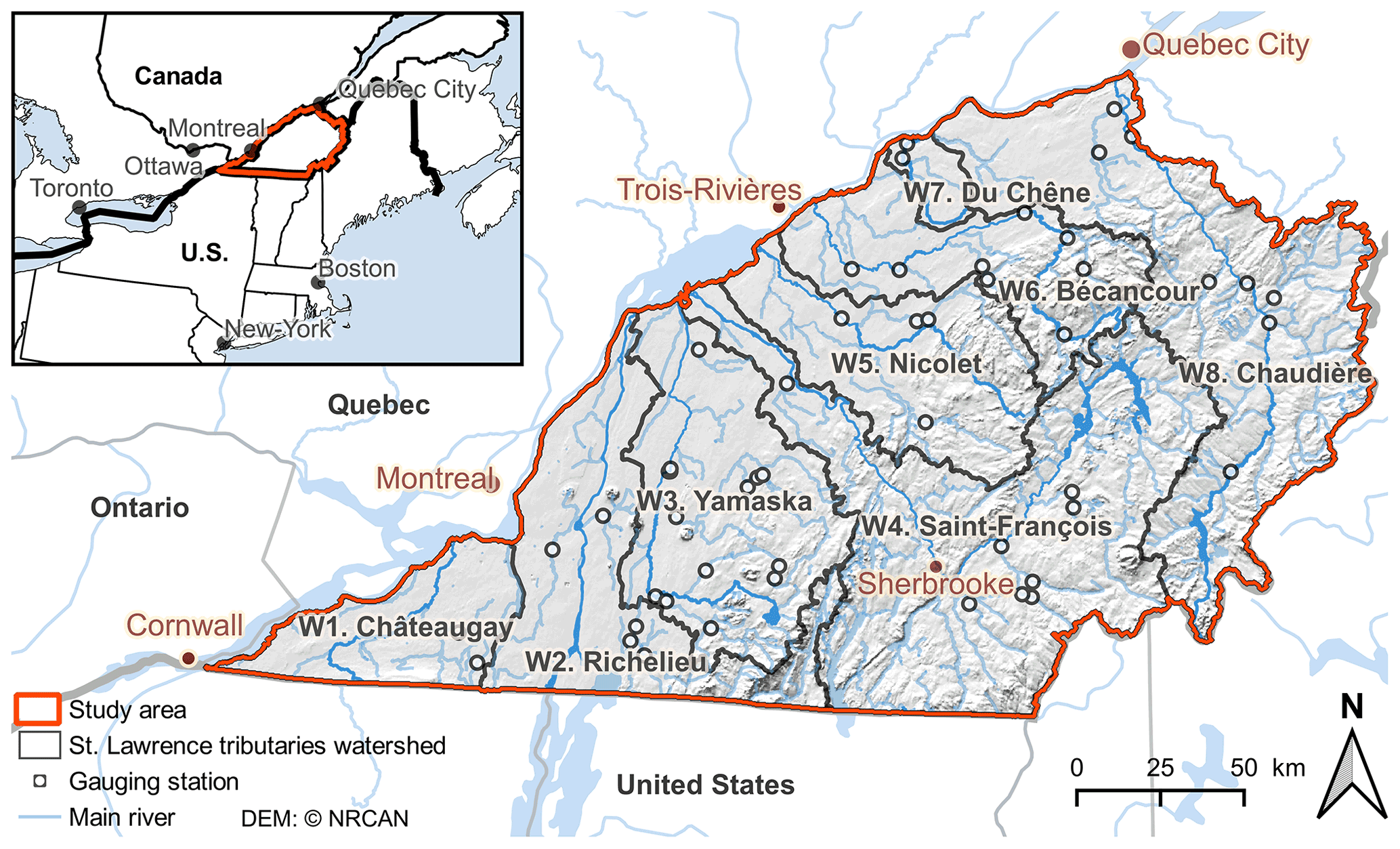
Figure 1Location of the study area and watersheds.
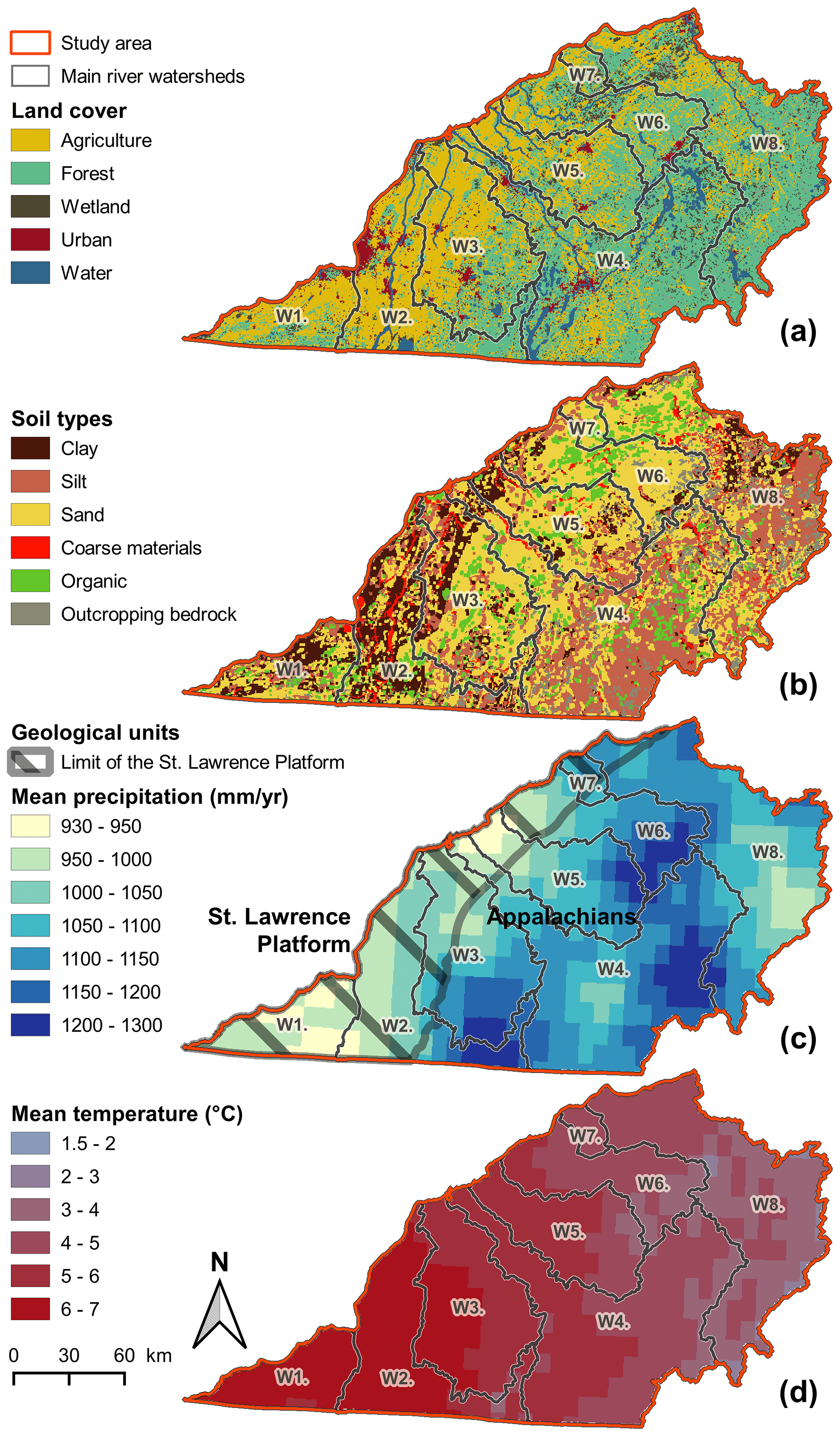
Figure 2(a) Land cover (reclassified from Bissonnette et al., 2016), (b) soil types (IRDA, 2008), (c) mean precipitation (1961–2017) as well as the areas of the St. Lawrence Platform (hatched) and the Appalachians, and (d) mean temperature (1961–2017) (Bergeron, 2016).
Table 1Characteristics of the studied watersheds.

* Part of the watershed is located in the USA – the presented values are for the Quebec part only.
Bergeron (2016) used 251 climate stations located in the study area to produce spatially interpolated temperature and precipitation data with a daily time step for the 1961–2017 period on a 10 km resolution grid. The high density of measurements during this period generated minimal error on the interpolated data, with a root mean square error (RMSE) of 3 mm/d for precipitation (mean bias of +0.1 mm/d), 2.5 ∘C for minimal temperature (mean bias of −0.5 ∘C), and 1.5 ∘C for maximal temperature (mean bias of +0.1 ∘C; Bergeron, 2016). Based on these data, average annual precipitation for the study area is 1090 mm (Table 1), including 275 mm falling as snow during winter (November to March). Precipitation is distributed relatively evenly throughout the year, and although total precipitation is similar for all of the watersheds, it is higher in the mountainous zones than in the lowlands (Fig. 2c). The average annual temperature is 5 ∘C (Table 1), with average monthly temperature varying between −15 ∘C (in January and February) and 20 ∘C (in July and August). Regionally, temperatures decrease from the southwest to the northeast (Fig. 2d).
The study area includes two main geological units: the sedimentary basin of the St. Lawrence Platform and the Appalachian mountain range (metasedimentary) (Malo, 2018; Fig. 2c). The bedrock of the St. Lawrence Platform is composed of slightly deformed Cambro-Ordovician fractured bedrock consisting of limestone, shale, and mixed shale and fine sandstone. The bedrock of the Appalachians is composed of highly deformed schist, quartzite, and phyllites (Thériault and Malo, 2018).
The bedrock is unevenly covered with unconsolidated Quaternary sediments from the last glaciation–deglaciation cycle, mainly composed of glacial, marine, fluvial, and lacustrine deposits. In this area, sediment depositional modes determine the geological nature of the superficial materials and the pedology (Fig. 2b). Thin (< 5 m) and relatively coarse superficial deposits (aeolian sands, till, and various glacial deposits) are found over the bedrock in the uphill areas. These deposits get thicker (5 to 20 m) in the valleys and in topographic depressions, with a wider mix of grain sizes resulting from the different depositional modes (fluvial, lacustrine, and marine). Closer to the St. Lawrence River, the thickness of the Quaternary deposits can reach several tens of meters, where silty clays from the Champlain Sea are covered with sandy materials (IRDA, 2008).
Regional fractured bedrock aquifers flow from the Appalachians to the St. Lawrence River (south/southeast to north/northwest). The aquifers are moderately productive and shallow, with the water table 3 to 5 m from the surface (Meyzonnat et al., 2018). They are in unconfined conditions upstream, where bedrock outcrops or under coarse superficial deposits, and reach semi-confined to confined conditions once the bedrock is covered by finer sediments in the valleys and close to the St. Lawrence lowlands (Rivera, 2014). Limited-extent shallow aquifers have been identified in the local superficial coarse deposits. Previous local or watershed-scale recharge studies have identified recharge areas upstream, mostly on the outcropping bedrock and in coarse glacial sediments, while the St. Lawrence tributaries drain groundwater over most of the study area. Gagné et al. (2018) showed that in the main GWR zones, the hydrogeological system has a rapid response, and most of the GWR rapidly reaches the nearby drainage system. The overall configuration corresponds to topographically driven water tables (Gleeson et al., 2011), with hydrogeological watersheds matching superficial watersheds, and can reasonably be considered to have a closed watershed water budget.
Daily flow rates are available from 51 gauging stations spread throughout the eight main tributary watersheds (CEHQ, 2019; Fig. 1), with watershed areas ranging from 30 to 3000 km2. Data missing for up to 5 consecutive days were linearly interpolated to optimize the length of the available time series. These 51 stations all have full-year measurements for more than 3 consecutive years, and the presence of ice most likely affects winter flow measurements.
3.1 HydroBudget
HydroBudget (HB; Dubois et al., 2021a) is a spatially distributed GWR model that computes a superficial water budget on grid cells of regional-scale watersheds with outputs aggregated into monthly time steps. The model uses commonly available meteorological data (daily precipitation and temperature, spatialized if possible) and spatially distributed data (pedology, land cover, and slopes). It is based on simplified process representations and is driven by eight parameters that need to be calibrated. These parameters are uniform over the grid and held constant through time (Table 2). Coded in R, HB uses a conceptual lumped reservoir to compute the soil water budget on a daily time step (Appendix A). For each grid cell and each time step, precipitation is divided between runoff (R), evapotranspiration (ET), and infiltration that could reach the saturated zone (potential GWR), with a monthly time step (Fig. 3; Dubois et al., 2021b).
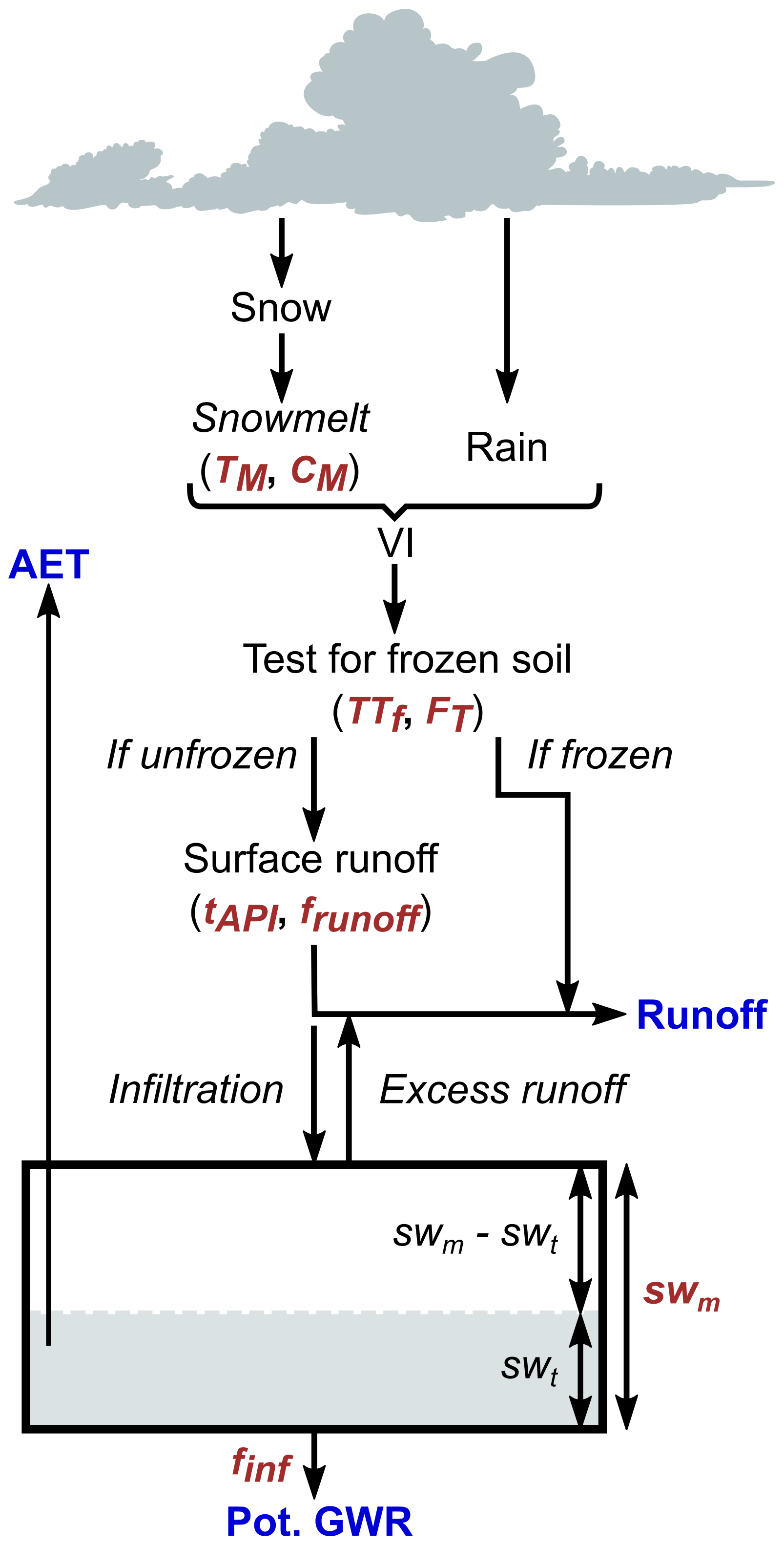
Table 2Description of the eight HydroBudget parameters.
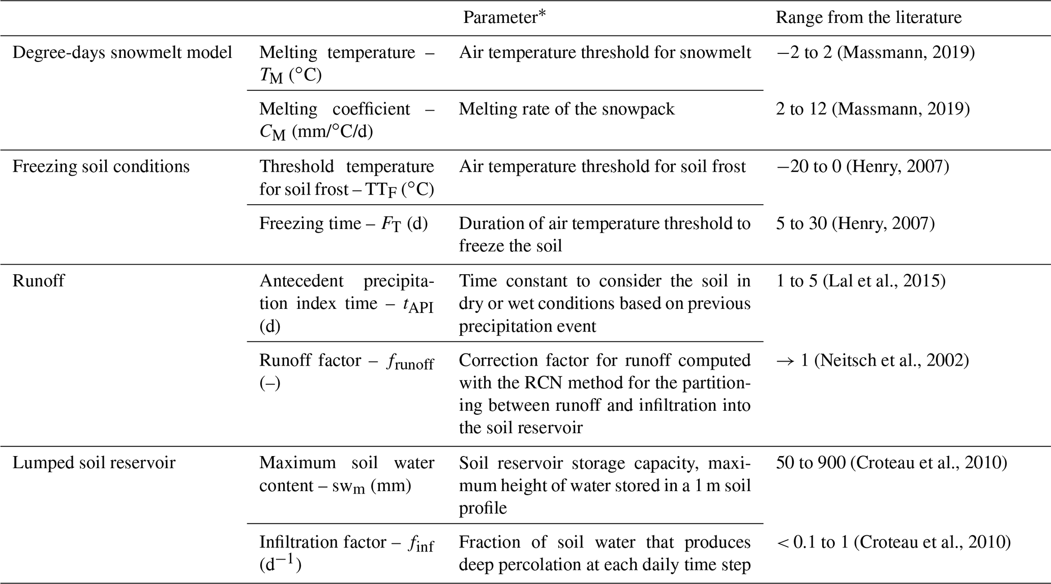
* Parameters are uniform over the grid and constant through time.
Calculations begin with the vertical processes by first determining the available liquid water (vertical inflow, VI), which is the sum of rain and snowmelt, with a 0 ∘C air temperature threshold for rain or snow and a two-parameter (TM and CM) degree-days approach (Massmann, 2019). If the soil is frozen (two parameters, TTF and FT), the entire VI will produce R directly. Otherwise, VI can flow as runoff, infiltration, evapotranspiration, and eventually percolation as potential GWR.
Runoff is calculated using the runoff curve number (RCN) method (USDA-NRCS, 2004, 2007) on a cell-by-cell basis (two parameters, tAPI and frunoff), similarly to what is done in the SWAT model (Arnold et al., 2012; Neitsch et al., 2002). The RCN is attributed per cell based on its pedology, land cover, and slope following the USDA-NRCS method adapted for the Quebec environment (Dubois et al., 2021b; Monfet, 1979). The remaining water (VI – runoff) is considered to be infiltration (I) reaching a soil reservoir for which storage capacity is driven by one parameter (swm). If I exceeds available storage, saturation excess is added to R. Otherwise, actual evapotranspiration (AET) is calculated as the minimum of PET (calculated using the formula of Oudin et al., 2005) and the available water in the soil reservoir. The residual soil water is mobilized as potential GWR (one parameter, finf) or stored for the next time step.
HydroBudget thus calculates potential GWR, the recharge that could reach the aquifer, if (1) the geological material below the soil horizon allows deep percolation to occur, (2) no additional storage or losses occur in the unsaturated zone below the soil, and (3) no significant groundwater evapotranspiration occurs (Doble and Crosbie, 2017). Actual GWR corresponds to the part of potential GWR that would reach the water table, and potential GWR is therefore a maximum.
3.2 Calibration strategy
The HydroBudget model is calibrated on superficial watersheds, based on the hypotheses that (1) surface watersheds match hydrogeological watersheds and that (2) the rivers drain unconfined aquifers. Under these conditions, for any given watershed, potential GWR should be similar to river baseflow at the outlet, and the sum of runoff and potential GWR should be equal to the total flow at the outlet. Dripps and Bradbury (2007) and Guay et al. (2013) have shown that results of GWR water budget models (SWB and HELP, respectively) compared better to groundwater flow models (GFLOW and CATHY, respectively) at the monthly time step than at a daily time step. Thus, runoff, AET, and potential GWR were computed with HB with a daily time step, and the results were aggregated on monthly time steps. Calibration and validation of the model and analysis of the results were all performed on the monthly aggregated results. Also, the calibration and validation of the model were performed under the hypothesis that no major land use change occurred during the simulation period (i.e., land use was held constant).
The daily river flow rates used for calibration were those from 51 gauging stations (Fig. 1). Baseflows were estimated from the flow rate time series following the proposition of Ladson et al. (2013) with the Lyne and Hollick filter (Lyne and Hollick, 1979) and using a stochastic calibration and 30 filter passes. To compare the effects of the baseflow filters on GWR simulation, baseflows were also estimated with the Eckhardt (2005) and Chapman (1991) filters for the gauging stations of W6. As aquifers generally discharge into superficial water bodies in southern Quebec, baseflows estimated with recursive filters are considered an acceptable proxy of GWR dynamics. Total flows and baseflows were divided by the area of the given watershed to provide flow values in millimeters per year and thus facilitate the comparison of calibration results between watersheds of very different sizes.
The model was simultaneously calibrated for all the gauging stations using the automatic calibration procedure of the R package caRamel (Monteil et al., 2020) to obtain a regionalized set of parameters. Up to 5000 model calls were used, with several successive optimizations to confirm the reproducibility of the results, as recommended by Monteil et al. (2020). Model performance was assessed using the Kling–Gupta efficiency (KGE) calculated with total monthly measured and simulated total flow (KGE) as well as monthly baseflow and monthly potential GWR (KGE). The KGE is preferred here over the Nash–Sutcliffe efficiency because it better represents the low-flow periods (Gupta et al., 2009). Each river flow time series was divided into a calibration period (first two-thirds) and a validation period (last third), therefore allowing the objective functions to be computed per period.
The caRamel algorithm (Monteil et al., 2020), a combination of the multi-objective evolutionary annealing simplex algorithm (MEAS; Efstratiadis and Koutsoyiannis, 2008) and the non-dominated sorting genetic algorithm II (ε-NSGA-II; Reed and Devireddy, 2004), automatically calibrated the eight HB parameters to maximize KGE and KGE values. The algorithm produces an ensemble of parameter sets (called generation) to run the model, downscales the generation to the parameter sets that optimize the objective functions, and creates a new set of parameters that produces better results. To produce new generations and ensure that the optimization tends toward a global maximum, the algorithm samples the parameter sets that individually maximize the two objective functions, KGE and KGE, samples the parameter sets that maximize the minimum values of the two objective functions, and increases the variance of each parameter.
The eight HB parameters were optimized for each gauging station, grouped by river watershed to save computational time (from 51 individual optimizations to 8 grouped optimizations producing 8 sets of calibrated parameters), such as
with (KGE the KGE obtained over a river watershed (group of gauging stations), (KGE the KGE obtained for a gauging station, Nws the number of gauging stations per watershed, (KGE the KGE obtained over a river watershed (group of gauging stations), and (KGE the KGE obtained for a gauging station.
Finally, the set of parameters that allowed one to reach the best compromise was chosen by identifying the highest mean KGE value (KGEmean):
The weights attributed to each objective function in KGEmean were arbitrarily chosen to select the calibrated parameter set that maximizes the reproduction quality of the baseflows, considered to be the proxy for GWR (KGE), without losing the benefits of the multi-objective optimization (Appendix Table A1).
The eight sets of eight calibration parameters were regionalized (uniform calibration parameters over the grid), using the normalized densities of stations per group (number of stations per square kilometer) as weights. The grid-wise uniform calibration parameters used for the simulation were obtained:
with xregionalized one of the eight calibration parameters regionalized, xws one of the eight calibration parameters optimized for the gauging stations of a river watershed, and areaws the area of the watershed (km2).
Finally, the 100 best compromises of each group of gauging stations were used to produce the 100 best regionalized parameter sets, and the HB model was run with these parameters, estimating uncertainty from the standard deviation.
3.3 Model sensitivity
Using the R package Sensitivity (https://CRAN.R-project.org/package=sensitivity, last access: February 2021), the Morris global sensitivity approach (Morris, 1991), enhanced by Campolongo et al. (2007), was performed for the eight groups of gauging stations and for the two objective functions, KGE and KGE. The analysis consists of randomly and individually changing the eight calibration parameters of the model (one model call per change) until all have been changed and starting again from a new combination of random values to measure the individual effects of the tested parameters, known as the elementary effects. A repetition represents one model call for an initial set of parameters followed by eight model calls, one for each parameter. A large number of repetitions (> 20) limits the convergence of the sensitivity measurement toward a local maximum. The n number of repetitions produces n number of elementary effects per parameter, the absolute values of which are averaged (μ*) to sort the parameters from most (highest μ* value) to least sensitive (lowest μ* value).
4.1 Model sensitivity and model calibration
The model sensitivity was obtained with 60 repetitions of the design for the eight groups of gauging stations, representing 540 model calls for each group. The relative sensitivity of the model varied markedly between the groups of gauging stations for the simulated river flow rates (Fig. 4a) but appears to be more constant for the simulated potential GWR (Fig. 4b). Flow rates were mostly sensitive to the snow-related parameters (TM and CM), except for the western watersheds, where the frunoff was more important. The simulated potential GWR was most sensitive to frunoff and least sensitive to snowmelt parameters (TM and CM) for all the watersheds. The ranking from the second- to fifth-highest sensitivity of potential GWR only slightly varied between groups of gauging stations. River flow rates and potential GWR clearly showed limited sensitivity to the soil freezing time (FT), with only a slightly higher sensitivity for the eastern watersheds W7 and W8. Overall, the potential GWR was more sensitive to parameter variations than river flow since all the μ* values for the river flow were lower by a factor 2 to 10 than for the potential GWR (values not presented here).
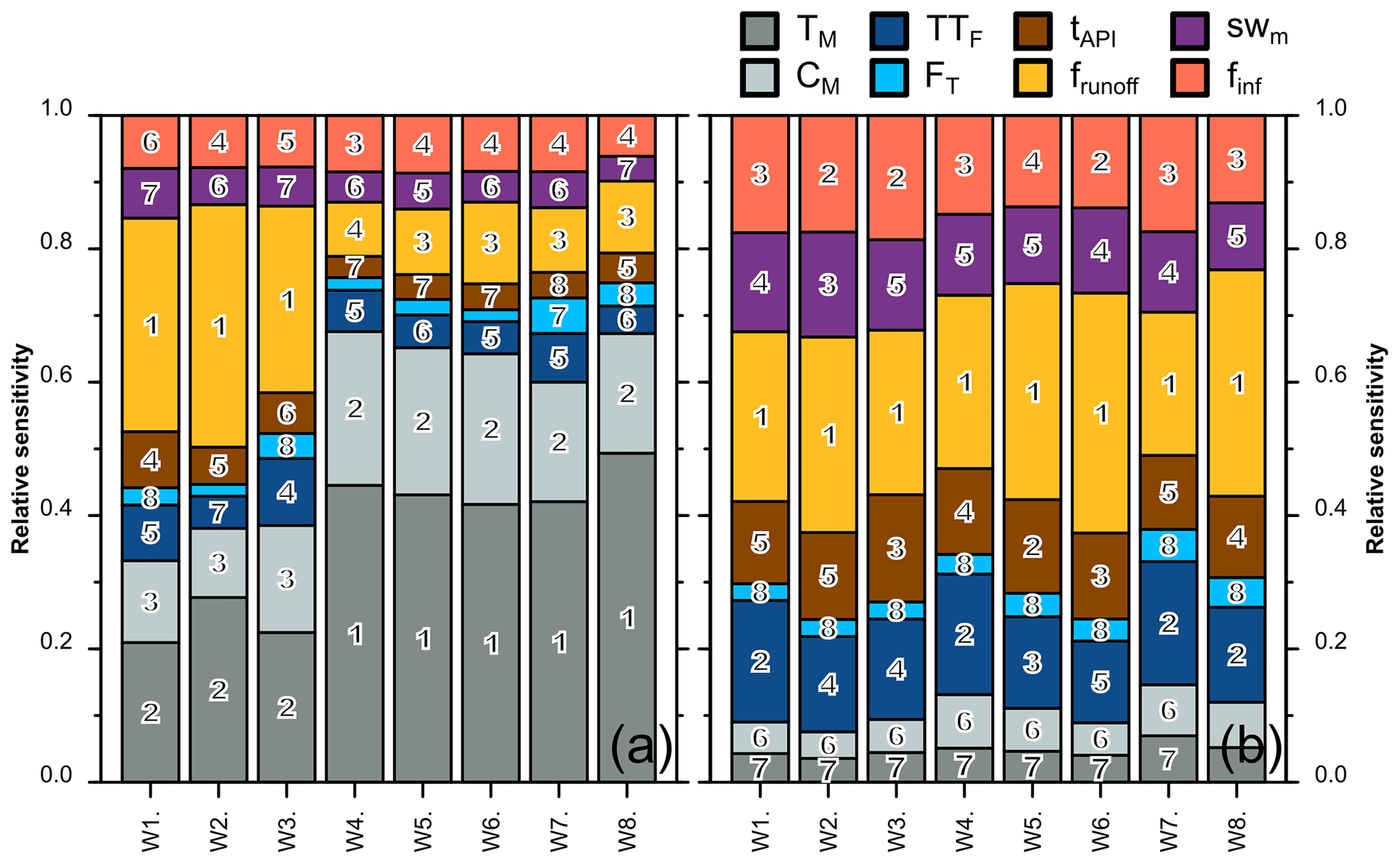
Figure 4Relative sensitivity of the eight model parameters to the simulated river flow rates (a) and to the simulated potential groundwater recharge (b) for the eight groups of gauging stations. The relative parameter ranking is reported in the bars from the most sensitive, 1, to the least sensitive, 8.
In a preliminary step, the calibration process was performed with the W6 (Bécancour) group of stations. Up to 5000 model runs were performed, and the 25 best compromises were extracted to compare the equifinality in the solutions. The KGEmean for this watershed varies within a range of ±0.005 in calibration and ±0.02 in validation (Appendix Table A1). Furthermore, the variability of the optimized parameters of the 25 best compromises was very limited, therefore allowing one to assume that the optimization per gauging station group converged. Calibration for this watershed was relatively short (e.g., 5 min for a 3380 km2 watershed, 500 m resolution grid (13 500 cells), for 57 years with 15 cores and 50 GB of RAM), and convergence was repeatedly attained before 1000 model runs. The objective functions, the calibrated parameters, and the interannual potential GWR values showed very limited sensitivity to the weights chosen for the computation of the KGEmean (Appendix Table A1). As the absolute value of baseflow changed with the filter method, the interannual GWR varied in consequence. The calibrated parameters with the different baseflow estimates slightly varied but remained in the parameter ranges described in Table 2. The objective functions were similar, between 0.7 and 0.8, except for KGE in validation, which was slightly lower with the Eckhardt (2005) and Chapman (1991) filters than with the Lyne and Hollick (1979) filter.
In light of these results, calibration of the rest of the gauging station groups was thus undertaken with 1500 model runs in order to save computational time. Also, the stochastic calibration and 30 passes of the Lyne and Hollick (1979) filter developed by Ladson et al. (2013) were retained for the baseflow estimate, and weights of 0.4 and 0.6 were associated with KGE and KGE, respectively, for the computation of KGEmean. Following regionalization, a satisfactory fit was observed between the calibrated model and measured flow rates and baseflows for all gauging station groups (Table 3). The KGEmean varied between 0.64 and 0.82 (average = 0.72) for the calibration period and between 0.62 and 0.77 (average = 0.69) for the validation period. The objective functions were very similar between the two periods, confirming the satisfactory calibration of the model and its capacity to reproduce the water budget over a long period, considering that calibration and validation span 1961 to 2017, and for the entire study area. The mean bias in simulated river flow rates and potential GWR varied between −9 and 5 mm/month (Table 3). The uncertainty computed with the 100 best regionalized parameter sets was ≤ 10 mm/yr for the three simulated variables (Table 4).
Table 3Objective functions for the simulated outputs, for calibration and validation periods, and for mean bias over the entire period of measurement.

* The presented values are for the stations of the watershed that are completely located in Quebec.
Table 4Simulated runoff, actual evapotranspiration (AET), and potential groundwater recharge (GWR) and uncertainty for the study area between 1961 and 2017 for annual values, winter, spring, summer, and fall and for the eight watersheds (W1 to W8).
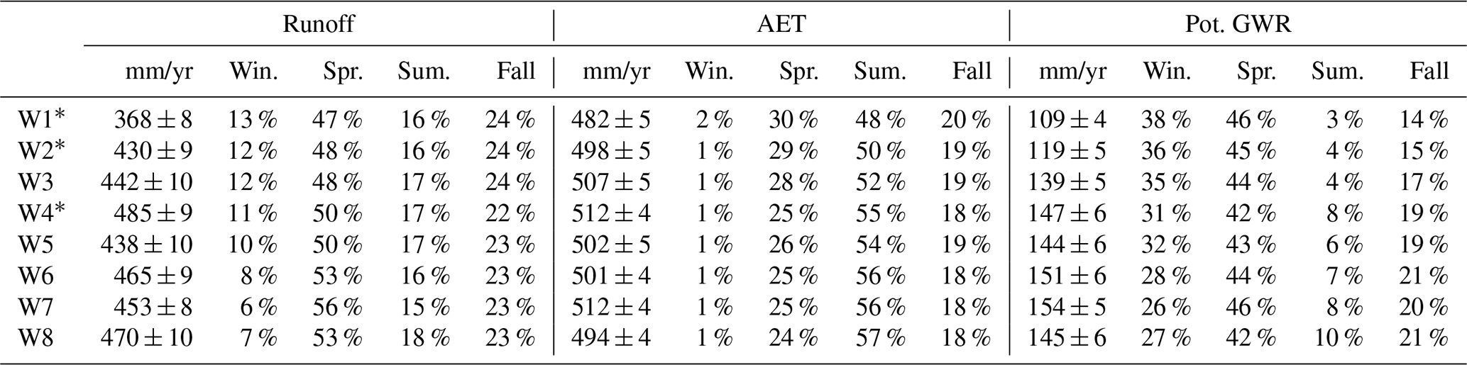
* Part of the watershed is located in the USA – the presented values are for the Quebec part only. Winter: December, January, February; spring: March, April, May; summer: June, July, August; fall: September, October, November.
4.2 Simulated potential groundwater recharge for 1961–2017
The calibrated HB model was used to simulate potential GWR for the entire study area on a 500 m × 500 m grid for the 1961–2017 period. Examples of the simulated monthly baseflows (Lyne and Hollick filter) and potential GWR are illustrated in Fig. 5 for the downstream stations in W3, W7, and W8. The simulated potential GWR compared favorably with baseflows estimated using the Lyne and Hollick (1979) digital filter. Maximum values were reached simultaneously in April, during the spring month(s) of maximum VI. A second baseflow and GWR peak was observed and simulated in November–December of most years. The lowest values were reached in July to September (high AET rates) and February (minimum VI). Similar matching results in timing and amplitude were obtained for the river flow (not presented here). Simulated AET was null in the winter until the spring thaw, after which it quickly reached its highest value (> 100 mm/month) in July and decreased at the end of August, reaching null values again in November. Comparable results were obtained for the other gauging stations (not shown).
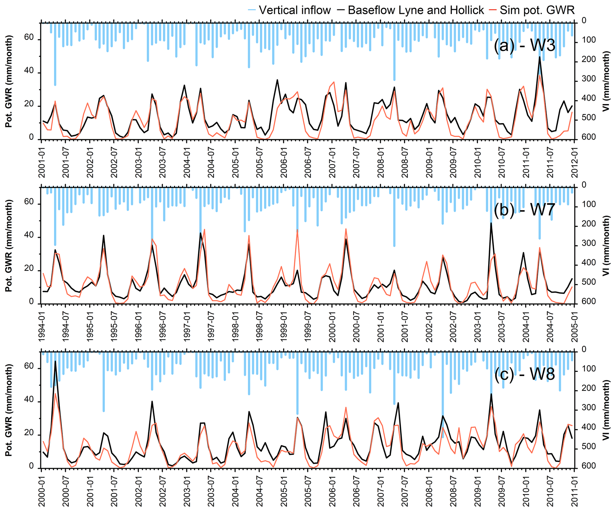
Figure 5Examples of simulated monthly potential groundwater recharge (GWR) and baseflows estimated with the Lyne and Hollick (1979) filter for the downstream gauging stations of W3 (a), W7 (b), and W8 (c).
The distribution of GWR rates showed a zone of low GWR rates (< 140 mm/yr) in the western part of the study area (flat and clayey St. Lawrence Platform), mainly in W1, W2 (except for its southeastern part), the central and northwestern parts of W3, and the northern part of W4, W5, W6, and W7 (Fig. 6a). A zone with higher GWR rates (140 to 280 mm/yr, locally > 280 mm/yr) covered the southern parts of W3, W4, W5, W6, and W8 (Appalachians). Areas of high GWR rates in the central parts of the study area (W2, W3, W4, W5, and W6) also corresponded to the zones of higher precipitation (Fig. 2c). The regional GWR–precipitation ratio (Fig. 6b) identified the areas of preferential recharge with ratios > 0.15, corresponding to areas of potential GWR rates > 140 mm/yr mainly located in the Appalachians (southern parts of W2 and W3 and W4 to W8). In the St. Lawrence Lowlands (W7 and lower portions of W4, W5, W6, and W8) and on the Appalachian Piedmont (central portions of W3), the ratios > 0.2 were associated with superficial coarse materials disconnected from the regional water table, meaning that the simulated potential GWR probably did not reach the fractured bedrock aquifer.
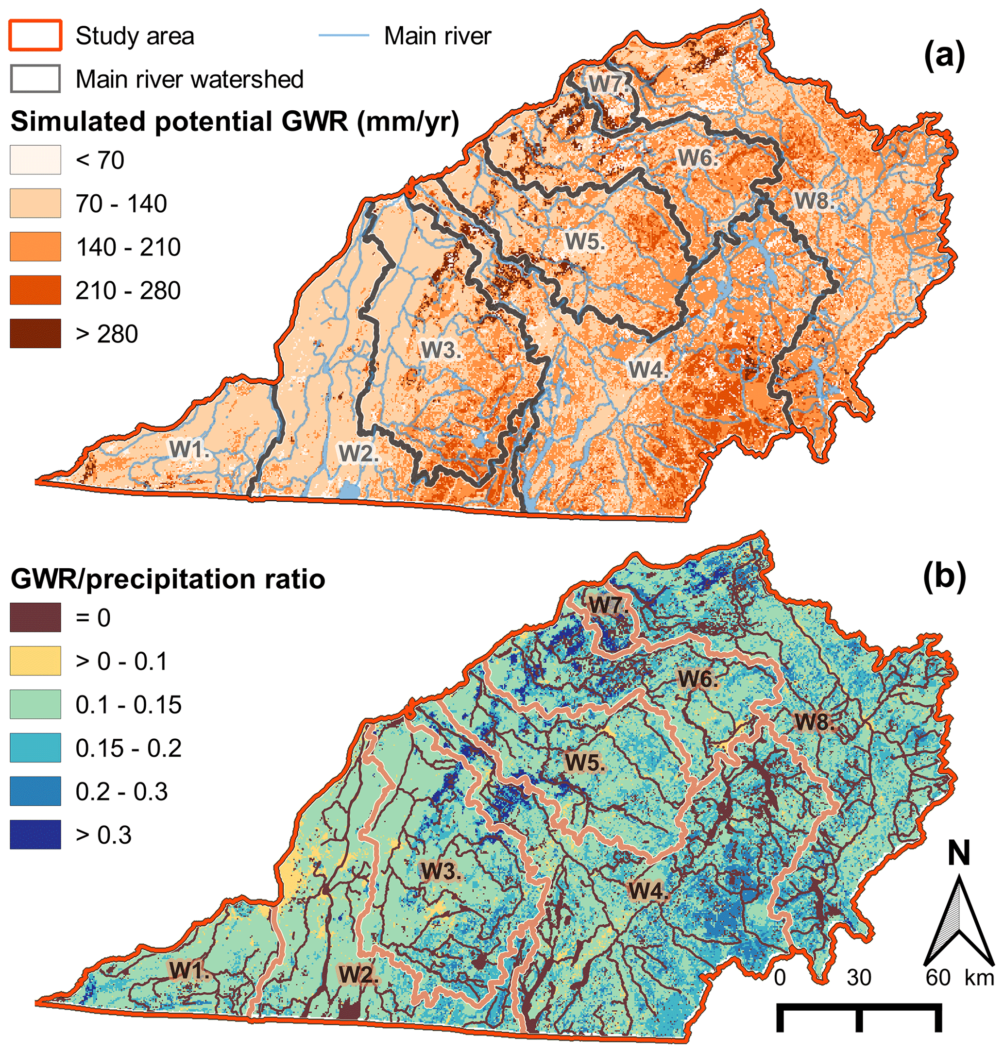
Figure 6(a) Average potential GWR simulated using the HydroBudget model for the study area between 1961 and 2017 and (b) GWR/precipitation ratio for the same period.
4.3 Partitioning and seasonality of the water budget
Across the study area, the average simulated runoff was 444 mm/yr (41 % of total precipitation), the average simulated AET was 501 mm/yr (47 % of total precipitation), and the average simulated potential GWR was 139 mm/yr (12 % of total precipitation) (Table 4). Mean annual GWR rates accounted for less than 140 mm/yr in watersheds mainly located in the St. Lawrence Platform (W1, W2, and W3 to a certain extent) and for more than 140 mm/yr for the watersheds mainly located in the Appalachians (W4 to W8), according to the two zones of high and low GWR rates previously described.
The seasonality of the water budget varied with more important winter runoff and potential GWR (and higher spring AET rates) in the western watersheds than in the eastern watersheds (Table 4). Summer and fall AET and potential GWR were less important in the western watersheds than in the eastern ones. Runoff and potential GWR clearly peaked during spring (51 % and 44 % of the annual value, respectively) due to the snowmelt event in all watersheds. These variations in seasonal proportions of each variable were driven by the regional temperature gradient (decreasing temperature from west to east).
Partitioning of runoff, AET, and potential GWR according to soil type showed maximum runoff rates for organic deposits, often associated with wetlands, and minimum rates over clay (Fig. 7a). The highest AET rates occurred over coarse sediment and the lowest rates over clay, while the highest potential GWR rates were found in coarse deposits and the lowest ones in clayey areas. Steepening slopes produced more runoff and a slight increase in potential GWR (not for slopes > 8 %) (Fig. 7b). The increase in GWR rates associated with steeper slopes can be linked to the presence of coarser material usually corresponding to glacial deposits on hillsides (high infiltration rates). Low runoff rates were associated with the flat and clayey areas of the St. Lawrence Platform, where annual precipitation is the lowest of the study area (Fig. 2c). A clear contrast was visible in the effect of land cover on the water budget (Fig. 7c), with the highest runoff rates over wetlands and the lowest ones in forested areas. The highest AET rates were found for wetlands, while the lowest ones were found for urban areas. The highest potential GWR rates were associated with forested areas and the lowest ones with wetlands.

Figure 7Median, 25th and 75th percentile, minimum, and maximum values for annual runoff, actual evapotranspiration (AET), and potential GWR throughout the study area between 1961 and 2017, classified as a function of (a) soil type, (b) slope, and (c) land cover.
4.4 Temporal evolution of the simulated water budget since the 1960s
HydroBudget simulated the temporal evolution of the water budget in the study area from 1961 to 2017, thus producing an exceptionally long simulated time series of runoff, AET, and potential GWR for the area (Fig. 8). The effect of interannual variability in precipitation appeared clearly in the simulated runoff, with low runoff rates (< 350 mm/yr) produced during the driest year and high runoff rates (> 550 mm/yr) produced during the wettest year (Fig. 8a, c). The simulated AET varied less than runoff, mainly between 450 and 560 mm/yr (Fig. 8d). Interannual variations of potential GWR were relatively high, ranging between 90 and 200 mm/yr, and seemed more influenced by precipitation than by temperature variations (Fig. 8e).
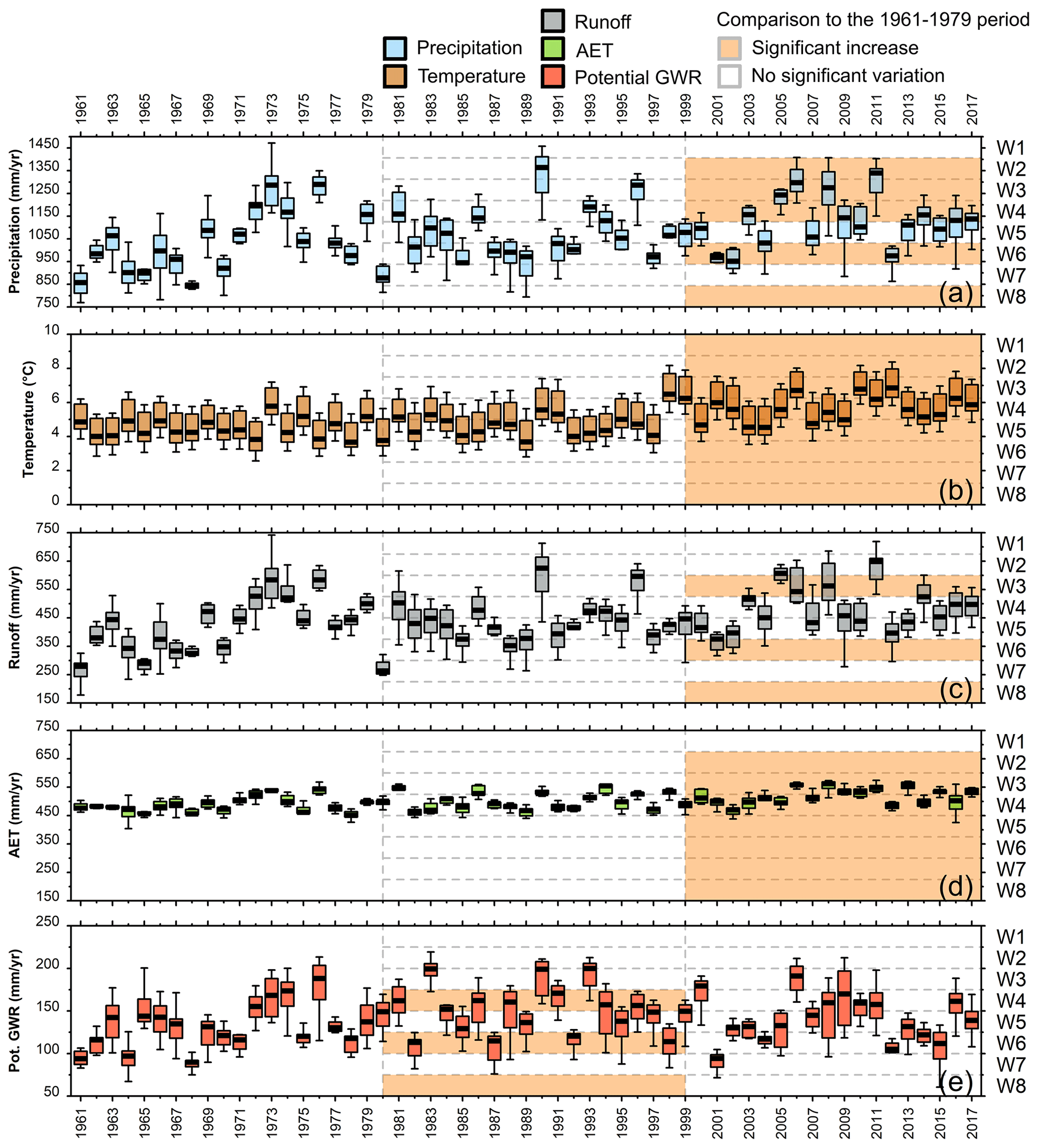
Figure 8Median, 25th and 75th percentiles, and minimum and maximum fluxes of (a) temperature, (b) precipitation, (c) simulated runoff, (d) simulated AET, and (e) simulated potential GWR and significant changes (Tukey test, p < 0.05) between the 1961–1979 period and the 1980–1998 and 1999–2017 periods for the eight watersheds (orange color).
The simulation period was split into three 19-year periods (1961–1979, 1980–1998, and 1999–2017) to look for significant changes in input variables (precipitation and temperature) and simulated variables (Tukey test, p < 0.05) (Fig. 8). Significant changes were found in the input variables between the 1961–1979 and 1999–2017 periods, with an increase in temperature for all watersheds and an increase in precipitation in five watersheds. These changes produced a significant increase in AET for all watersheds except W1 and an increase in runoff for three watersheds (W3, W6, and W8). However, these changes in precipitation and temperature did not impact the annual potential GWR, for which significant increases were simulated between the 1961–1979 and 1980–1998 periods only for W4, W6, and W8.
When considering the entire period (1961–2017), VI significantly increased (Mann–Kendall test, p < 0.05) annually for all watersheds except W5 and W7 and during winter (December to February) and summer (June to August) for all watersheds except W1 and W7 during summer (Appendix Table A2). Significant annual and seasonal temperature increases were also observed for all watersheds and for all seasons except W5 and W6 during spring. Similarly to VI, runoff significantly increased annually for all watersheds except W5 and W7 and during winter and summer for all watersheds except W1 during summer. Significant increases in AET were also simulated for annual values and during winter and spring, and unlike temperature, summer and fall AET showed no significant trend except for W6 and W8 during summer. Significant increases in potential GWR were simulated only for winter values for all watersheds except W1. Interestingly, although increasing runoff and AET were observed throughout the simulation period (1961–2017), no decreasing trends were simulated in potential GWR.
5.1 Regional groundwater recharge dynamic in cold and humid climates
Although river flows are well monitored by an extensive gauging station network over long periods, groundwater-level monitoring was initiated in the Province of Quebec only at the turn of the century (MELCC, 2020). Recharge estimates from these time series are yet to be produced. Moreover, a regional-scale lysimeter network still needs to be implemented. Local ground truthing of HB simulation results is thus limited by the lack of spatially distributed GWR estimates from alternative field-based measurements, restricting the verification of model results to comparisons with local field and modeling studies.
The average simulated potential GWR for the study area (139 mm/yr; 12 % of annual precipitation) is comparable to values found in previous studies in the region. For example, Chemingui et al. (2015) used the CATHY integrated hydrological model in W1 to estimate GWR to be 200 mm/yr. Although this value is much higher than the one obtained using HB in the same area (109 mm/yr), the resulting preferential recharge areas located close to the Canada–USA border are similar with both approaches (i.e., 70 to 250 mm/yr in Chemingui et al., 2015, and 70 to 280 mm/yr with HB). The average recharge rates simulated using the HELP model, also calibrated using flow rates and baseflow estimates, are similar to the HB-simulated potential GWR rates in two watersheds of the study area: 86 mm/yr for W1 (Croteau et al., 2010) and 185 mm/yr for W8 (Benoit et al., 2014) compared to 109 mm/yr and 145 mm/yr with HB, respectively. Using the WaterGAP Global Hydrology Model (WGHM; Döll et al., 2003) and a 0.5∘ spatial resolution, Döll and Fiedler (2008) found GWR rates ranging from 100 to 300 mm/yr in southern Quebec, thus generally matching the range of HB-simulated GWR. Wada et al. (2010) simulated much higher GWR rates over the study area (300 to 1000 mm/yr) with the global hydrological model PCR-GLOBWB (Bierkens and van Beek, 2009) at a 0.5∘ spatial resolution. These values do not match HB estimates, nor do they match any other results for the study area.
The spatially distributed potential GWR values show a clear difference between areas in the St. Lawrence Platform (GWR < 140 mm/yr) and areas in the Appalachian geological units (GWR > 140 mm/yr). Higher recharge occurs when soils are coarser or in outcropping bedrock areas, which are mostly located in the Appalachians and upstream in the watersheds, in accordance with what has been found in previous studies (Benoit et al., 2014; Croteau et al., 2010; Levison et al., 2014). Spatial variations in GWR also correlate well with land use, with preferential infiltration zones in forested areas and lower infiltration rates over wetlands and urban areas. Overall, local surface conditions, such as soil type and land use, mostly influence GWR rates. Similar results of factors influencing GWR are reported by Batelaan and De Smedt (2007) and Zomlot et al. (2015) in Belgium (oceanic climate) and by Nielsen and Westenbroek (2019) in Maine (USA – cold and humid climate).
Within the study area, potential GWR occurs mainly in the spring (44 %) and winter (27 %–38 %), while almost no GWR occurs in the summer (3 %–10 %), and a moderate contribution occurs in the fall (14 %–21 %). Differences between watersheds in this seasonal dynamic seem to be driven by the southwest–northeast decrease in temperatures, with higher winter GWR rates obtained in the warmer western watersheds and higher summer and fall GWR obtained in the colder eastern watersheds. Similar observations can be made for runoff and inversely for AET.
This spatiotemporal link between GWR and precipitation and temperature patterns is coherent with that reported in other studies. For example, Dierauer et al. (2018) used river flow observations of 63 streams in the Rocky Mountains (Canada and USA, snow-dominated hydrology) to link winter conditions to GWR. The proportion of total precipitation occurring in winter and winter temperature were identified as important variables for the variability of winter and summer low flows. The seasonality of GWR is well documented in the humid conditions of northern Europe as well, with an increase in the importance of winter events (rain-dominated GWR) at the expense of the spring snowmelt (snow-dominated GWR) with the increase in average temperature from north to south (Kløve et al., 2017; Nygren et al., 2020).
Simulated GWR from the current study is inversely correlated with AET, occurring preferentially when AET is low, immediately following snowmelt and before the onset of soil frost. Similar results are reported from other cold and humid climates (Grinevskiy et al., 2021; Kløve et al., 2017; Okkonen and Kløve, 2011; Nygren et al., 2020). The importance of snowmelt-related recharge evidenced by the simulations has also been observed using field data. Using isotopic analyses, Jasechko et al. (2017) have shown that high proportions of total GWR occurring during winter were associated with the amount of winter precipitation in central Canada and worldwide with preferential infiltration periods during the cold months (Jasechko et al., 2014). Wright and Novakowski (2020) have linked increases in groundwater levels from observation wells to GWR events in the neighboring Province of Ontario (Canada) during rain-on-snow and partial thaw events, despite the presence of a frozen soil. They underline the importance of winter recharge events in seasonally frozen environments and their potentially increased importance in a warming climate.
5.2 Trends in groundwater recharge in cold and humid climates in the past decades
Warming temperatures have been recorded in the cold and humid climates of the Northern Hemisphere since the middle of the 20th century. Mean annual temperature increased by +2 to +3 ∘C between 1954 and 2003, and this increase was more marked between December and February (up to +4 ∘C for the same period) (Arctic Climate Impact Assessment, 2004). In eastern Canada, temperature warming up to +1 to +3 ∘C has been identified for the 1948–2016 period (Vincent et al., 2018), leading to important changes in the seasonal distribution, and particularly to an increase in winter precipitation and a decrease in accumulated snow during the cold season (Kong and Wang, 2017). This work has shown that although the simulated potential GWR was not impacted by the long-term increases in precipitation or temperature on an annual time step for the 1961–2017 period, these changes produced significant increases in annual runoff and AET and may not have been sufficient yet to propagate to potential GWR. As observed with past data for winter trends in potential GWR, under changing climate conditions, seasonal and monthly GWR could increase during periods with more available liquid water and low AET rates (late fall, winter, early spring). Inversely, GWR could decrease for periods of enhanced AET rates (warmer temperature) such as late spring, summer, and early fall.
In Canada, other authors have looked for trends in observed time series of groundwater levels for the snow-dominated region of British Columbia (Allen et al., 2014) or across the country (Rivard et al., 2009), but each time, no coherent pattern could be identified. This could be due to short time series or insufficient data coverage. In western Russia, Grinevskiy et al. (2021) simulated an increase in GWR between the 1965–1988 and 1989–2018 periods with a surface energy balance coupled to the Hydrus unsaturated zone model. The GWR increase was due to a warmer winter, leading to a decrease in soil frost depth and an increase in the winter soil-water storage. Interestingly, the warming temperatures did not produce AET increases, which was interpreted to be due to a sharp decrease in wind speed. Inversely, Nygren et al. (2020) identified a significant decrease in groundwater depth time series across Finland and Sweden between the 1980–1989 and 2001–2010 periods. These authors showed that the deeper groundwater levels were linked to decreasing GWR patterns associated with shorter snowmelt periods and longer periods of intensive evapotranspiration. In comparison, the temperature increase observed in southern Quebec over the 1961–2017 period was probably not large enough to produce such a change.
An outcome of this work was to show that the regional long-term potential GWR simulations with a water budget allowed identification of the impacts of a changing climate on the past GWR conditions by positioning the trends (or absence of significant trends) in the globally changing hydrologic dynamic. Also, it emphasized the high responsivity of the hydrologic dynamic of the cold months to the climate changes in the cold and humid climates.
5.3 Implications for water management
This study has shown that the use of a GWR water budget model relatively easily produced long-term spatially distributed GWR values at the regional scale, with an acceptable spatial resolution and monthly time steps. The average GWR rate for the region, based on the new regional estimate, is 139 mm/yr, with lower aquifer renewal rates in the St. Lawrence Platform (< 140 mm/yr) than in the Appalachians (> 140 mm/yr). Preferential infiltration areas correspond to forested areas (170 mm/yr) and areas covered by coarse sediments (180 mm/yr) or outcropping bedrock (150 mm/yr). The decreasing temperature from west to east impacts the intra-annual GWR dynamic, imposing higher winter GWR in the warmer watersheds, from 38 % of annual recharge in W1 to 27 % in W8. Inversely, summer and fall GWR rates are lower in the western watersheds (3 % and 14 %, respectively, in W1) than in the eastern watersheds (10 % and 21 %, respectively, in W8). Furthermore, the warming temperatures since 1961 did not negatively affect GWR until 2017, due to a simultaneous increase in precipitation and higher winter GWR, compensating for the increase in AET. However, with more intense and faster climate change, this dynamic could change in the near future if temperature warming was to exceed precipitation increase.
Based on the study results, GWR maps should be included in land management planning to avoid impacting areas of preferential recharge, such as forests, areas covered by coarse material, and zones of outcropping bedrock. Although the GWR–precipitation ratio in eastern North America seems to be 0.25 and higher (Jasechko et al., 2014, based on the global simulation of Wada et al., 2010), areas of preferential recharge can be identified in the study area based on a GWR–precipitation ratio higher than 0.15 (the worldwide mean in Jasechko et al., 2014). These represent essential areas for the quantitative replenishment of groundwater resources and therefore the most vulnerable areas in terms of water quality of southern Quebec. Forested areas should be prioritized for future preservation and forest conservation policies implemented for groundwater resource protection. Although it has been shown that wetlands are often connected to the water table in southern Quebec (Bourgault et al., 2014), they are not considered to be preferential infiltration areas in HB. Separate studies will be necessary to investigate their role in regional groundwater flow. Considering the substantial influence of winter on the regional hydrology, one of the novel outcomes of this study, and that changes in the winter dynamic could highly influence the entire hydrologic dynamic of cold regions (Jasechko et al., 2014, 2017), additional winter-related research should target gauging of winter river flows, soil frost modeling, and enhancing the vertical inflow and snowpack modeling and would probably require the development of the winter monitoring network.
It is important to underline that actual GWR is most likely lower than potential GWR, especially where superficial deposits are thick and have low hydraulic conductivity or where impermeable sediments are present at depth and may induce confined conditions for underlying aquifers. To overcome this, Rivard et al. (2013) and Gagné et al. (2018) applied a 40 % reduction coefficient in the semi-confined areas of W5 to estimate actual GWR from potential GWR and assumed that no recharge occurred over confined aquifers.
5.4 Contributions to and limitations of water budget models in groundwater recharge simulation
HydroBudget was specifically developed to simulate spatial and temporal variations in potential GWR at the regional scale, for long periods and for regions where winter largely affects the intra-annual hydrologic dynamic. The model can reasonably be used where hydrogeological and superficial watersheds are similar, where regional groundwater flow converges to rivers, and when a monthly resolution is sufficient. Although the model does not compute water routing, groundwater–surface water feedback, or evapotranspiration from groundwater, and produces potential GWR, the satisfying simulation results found in this work justify the water budget calculation scheme used in HB, resulting in an easy-to-use and computationally efficient model. Furthermore, the uncertainty analysis showed that the calibration method provides an interestingly small uncertainty for the simulated variables and a mean bias similar to that of the input data.
The impact of long and cold winters was included in HB through the widely used degree-days method that represents snowpack evolution (Massmann, 2019) and through the representation of freezing soil conditions with a threshold temperature and a duration of the threshold temperature to freeze the soil (TTF and FT, respectively). The results showed that the simulated potential GWR was sensitive to TTF, while both flow rates and potential GWR had limited sensitivity to FT (Fig. 4). The colder watersheds were more sensitive to these parameters, while the simulations of river flows in the warmer watersheds were less sensitive to the snow-related parameters. These results underline the importance of including soil freezing in GWR modeling for cold regions, as did other studies in cold and humid climates (Grinevskiy et al., 2021; Nemri and Kinnard, 2020; Okkonen and Kløve, 2011). This work pinpoints the need for more research on winter recharge to better understand the processes involved.
Several existing water budget models (HELP; HydroBudget; SWB; water balance GIS tool; Huet et al., 2016) use the RCN curve number method (USDA-NRCS, 2004) as a simplification for runoff calculation. This method, developed specifically for the US context, has been criticized for its empirical basis (Ogden et al., 2017). However, it is continuously adapted and used for new environments and different size areas and is well documented and easy to use (Bartlett et al., 2016; Lal et al., 2015; Miliani et al., 2011; Ross et al., 2018). Notably, it is used to estimate runoff in the SWAT hydrological model (Neitsch et al., 2002) and is calibrated specifically in the Quebec climate and geological context (Gagné et al., 2013; Monfet, 1979). In water budget models, the RCN method drives the partitioning of the simulated water budget into runoff and water available for AET and GWR, therefore making the related parameters (tAPI and frunoff) particularly sensitive in their simulation (e.g., frunoff is the most sensitive parameter for potential GWR in HB; Fig. 4). Because it is based on land cover, topography, soil types, and seasonal humidity, the RCN method reflects the spatial variability of the large study area, which probably contributes to the ability of HB to simulate the surficial water budget and discriminate its partitioning depending on the superficial conditions (superficial geology, land cover).
The AET corresponded to 47 % of the annual precipitation (501 mm/yr), a result similar to those reported in previous work in the study area (Benoit et al., 2014; Croteau et al., 2010; Guay et al., 2013). Considering the vegetation cover of southern Quebec (45 % of the area of forest and 6 % of wetlands), its relatively large water availability, with an average of 1090 mm/yr of precipitation evenly distributed throughout the year, the topography-driven water table, and the shallow depth of the aquifers, groundwater–vegetation–atmosphere exchanges are probably intensive (Koirala et al., 2017; Xu and Liu, 2017). The configuration of the HB model, with a soil lumped reservoir for AET–potential GWR partitioning, is therefore conceptually suitable (Cuthbert et al., 2019). AET computation is driven by two parameters, i.e., the runoff factor (frunoff), influencing the partitioning between runoff and infiltration into the soil reservoir, and the soil reservoir parameter (swm), determining the reservoir capacity. Evapotranspiration calibration data would be useful to better constrain these two parameters, but measured values are rarely available for this variable.
The simulated transient GWR was calibrated with baseflows computed using regressive filters from river flow rate time series. Although Partington et al. (2012) showed that the association between baseflows and GWR is not always satisfactory and that different baseflow separation methods can lead to differences in volumes and timing (Gonzales et al., 2009; Zhang et al., 2017), baseflows are generally considered an acceptable proxy for GWR in cold and humid climates (Chemingui et al., 2015; Dierauer et al., 2018; Rivard et al., 2009). They are widely used for the calibration of GWR simulations (Batelaan and De Smedt, 2007; Croteau et al., 2010; Dripps and Bradbury, 2007; Gagné et al., 2018; Rivard et al., 2013). In this work, using baseflow estimated with the Lyne and Hollick (1979), Eckhardt (2005), and Chapman (1991) filters influenced the proportion of baseflow in total river flow and consequently led to variations in simulated potential GWR (Appendix Table A1). However, the quality of the simulations was comparable due to parameter variations that remained in the possible range of the parameters (Table 2).
Having a model that is fully coded in an open-source language leaves the option of reshaping its structure and conceptual model to specific study needs and environments. Changes to the model could include, for example, changing the PET calculation to a formula considered to be more suitable for a specific local context, defining a different runoff computation method that would better represent local conditions, modifying the representation of the soil reservoir by spatializing it, or using other calibration data, such as observation of AET or other baseflow filters. However, it should be kept in mind that increasing the complexity of the process representation would increase the number of parameters to be calibrated and most likely increase computation time as well. An original contribution of this work was to show that the tested calibration method combined with a regionalized parameter set offers a very acceptable solution that is highly reproducible and could be applied in less monitored regions. Apart from being relatively simple to use, the HB model has high potential for non-hydrogeologist users, especially if the computational time is limited and the update of observation data and the automatic calibration procedure are easy tasks. Hydrogeologist modelers might be interested in including HB as a complementary tool for comparative purposes when using integrated models or when in need of GWR estimates for groundwater flow models.
Groundwater recharge is a strategic hydrologic variable that needs to be estimated for sustainable groundwater management, especially within the global warming context that highly impacts winter conditions in the cold and humid climate regions. It is a challenge to simulate groundwater recharge at the regional scale and for long-term conditions because of long computational times and the large number of calibration data required to produce reliable results, especially because groundwater observations often remain too scarce for such spatiotemporal scales. The objective of this study was to demonstrate the relevance of using a water budget model to understand long-term transient and regional-scale GWR in cold and humid climates where groundwater observations are scarce. As a typical case study, the HydroBudget model was automatically calibrated with river flow rates and baseflow estimates to simulate long-term regional-scale GWR in the cold and humid climatic conditions of southern Quebec. With the model simultaneously calibrated on 51 gauging stations, GWR was simulated between 1961 and 2017 at the regional scale (36 000 km2) with very little uncertainty (< 10 mm/yr). GWR estimates at this scale, including eight tributary watersheds of the St. Lawrence River with a monthly time step and 500×500 m resolution, were not available until now. The study demonstrated that the ability of the HB model to simulate snowpack evolution and soil frost appears to be a key feature for GWR simulation. Another outcome of this work was to show that the model sensitivity to its parameters is correlated with the average air temperature of the watershed, making the simulated water budget in watersheds with lower temperature more sensitive to snow-related parameters than the warmer watersheds. Nevertheless, additional research focusing on snow melting and freezing soil processes would help to better constrain the model for the winter and spring periods, consequently helping better anticipate future changes.
Water budget partitioning has proven to be highly useful for linking changing climatic conditions to trends and evolution in regional GWR in the last 6 decades. The water budget is partitioned into runoff (41 %, 444 mm/yr), AET (47 %, 501 mm/yr), and potential GWR (12 %, 139 mm/yr). This study shows that groundwater recharge peaks in the spring (44 % of annual recharge) and is high during winter (32 % of annual recharge). Interestingly, the long simulation period made it possible to identify a significant increasing trend of GWR during winter and no decreasing trends during summer, despite warmer temperatures. This is most likely because increases in AET are compensated by increases in precipitation. In contrast to previous studies of past GWR trends in cold and humid climates, this work has shown that changes in past climatic conditions have not (yet) produced significant changes in annual potential GWR but have impacted runoff and AET. However, considering the intense and fast climate change expected in future decades, the water budget partitioning and the regional GWR could decrease if temperature warming were to exceed the increase in precipitation.
Besides providing essential long-term and regional-scale data on regional GWR, a water budget model with a relative ease of use, such as HB, and that can be calibrated regionally with available data can be extremely useful for non-hydrogeologist users from water management and environmental agencies. It can be used to implement water resource conservation policies, anticipate the impacts of climate change, and identify additional research required.
Equations used in the HydroBudget model (adapted from Dubois et al. (2021b), the eight calibration parameters, uniform over the grid and constant through time, are identified with bold characters).
A1 Degree-days snowmelt model
Determining whether the temperatures generate snowfall.
Determining whether the temperature generates snowmelt, calculating snowmelt and VI.
t is the current daily time step, Tt is the air temperature (∘C), snowfallt is the snowfall in snow water equivalent (mm), is the total precipitation (mm), TM is the melting temperature (∘C), snowpackt is the snowpack in snow water equivalent (mm), snowpackt−1 is the snowpack in snow water equivalent at the previous time step (mm), snowmeltt is the liquid water produced by snowmelt (mm), CM is the melting coefficient (mm ∘C−1 d−1), and VIt is the vertical inflow (mm).
A2 Runoff computation
Computing the antecedent soil conditions.
Computing the values of RCN for dry and humid soil conditions based on equations from Monfet (1979).
Adjusting the RCN value based on the antecedent soil conditions.
Computing runoff (with conditions on the soil frost).
APIt is the antecedent precipitation index (mm). tAPI is the antecedent precipitation index time (d). RCN is the computed value of the runoff curve number for the considered pixel (–). frunoff is the runoff factor (–). RCNdry is the corrected value of the runoff curve number for dry soil conditions (for the Quebec environment) (–). RCNwet is the corrected value of the runoff curve number for humid soil conditions (for the Quebec environment) (–). RCNt is the considered value of the runoff curve number for the time step (–). FT is the freezing time (d). TTF is the threshold temperature for soil frost (∘C). Rt is runoff (mm).
A3 Lumped soil reservoir
Computing infiltration as runoff excess.
Computing saturation excess.
Computing the AET based on the soil water content.
Computing the potential GWR based on the soil water content after the AET computation.
Inft is infiltration to the soil reservoir (mm). swm is maximum soil water content in the soil reservoir (mm). sw't−1 is soil water content at the end of the previous time step (mm). Excess Rt is saturation excess produced by the soil reservoir (mm). Total Rt is total runoff (mm). PETt is potential evapotranspiration (mm). AETt is actual evapotranspiration (mm). swt is soil water content after the AET computation (mm). GWRt is potential GWR (mm). finf is the infiltration factor (d−1). sw't is soil water content after the AET and GWR computation (mm).
A4 Model output per grid cell
Rm is simulated monthly total runoff (mm), n is the number of days in the considered month, AETm is simulated monthly AET (mm), and GWRm is simulated monthly potential GWR (mm).
Table A1Best compromises, interannual potential GWR, and optimized parameters obtained with the best compromises for the gauging stations of W6 and ranges obtained with the 25 best compromises (before regionalization) using different calibration weights and different baseflow separation methods.
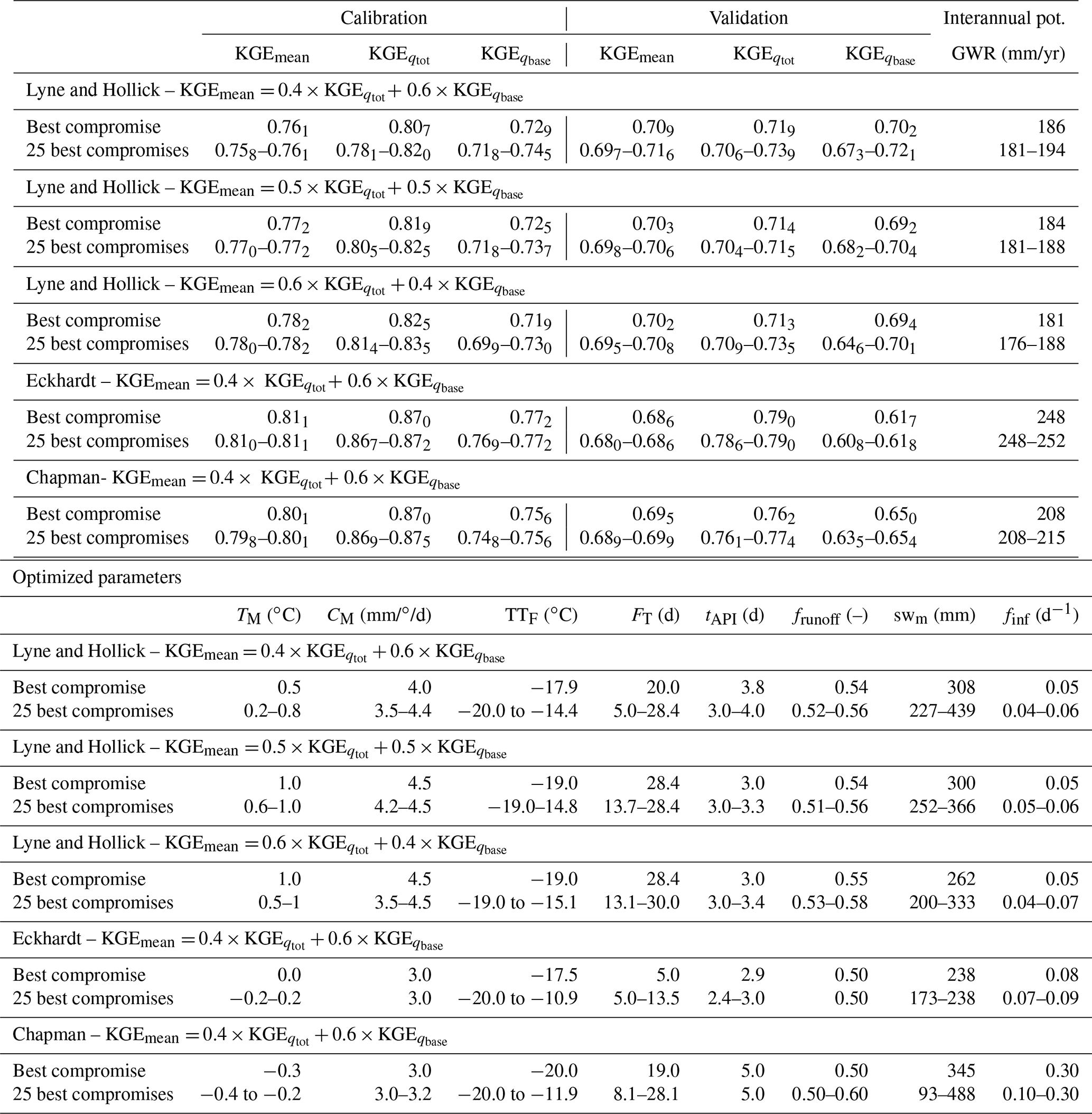
Table A2Annual and seasonal trends for vertical inflows (rain plus estimated snowmelt), observed temperatures, simulated runoff, simulated actual evapotranspiration (AET), and simulated potential groundwater recharge (GWR) for the 1961–2017 period for the eight watersheds (Mann–Kendall test; only p values > 0.05 are presented, otherwise a “–” is used; all trends are positive).
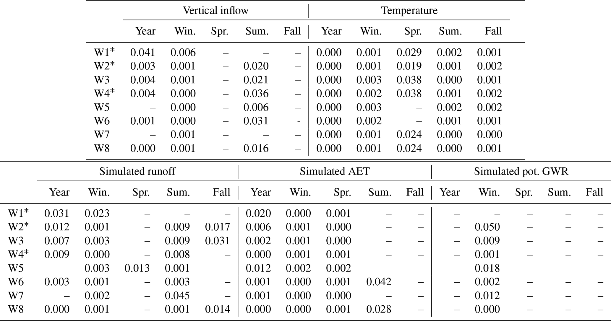
* Part of the watershed is located in the USA – the presented values are only for the Quebec part.
The script of the HydroBudget model is open source and can be downloaded with an application example from https://doi.org/10.5683/SP3/EUDV3H (Dubois et al., 2021a).
The simulated variables in this work are available here: https://doi.org/10.5683/SP3/TFNPQF (Dubois et al., 2021c).
ED, ML, and SG contributed to developing the approach, and all the authors contributed to writing the paper. ED and SG developed the HB script in R, based on the model created by GM, which was implemented in Java script. Data management, simulations, and figure preparation were done by ED. ML obtained the research grant and supervised the research.
The contact author has declared that neither they nor their co-authors have any competing interests.
Publisher's note: Copernicus Publications remains neutral with regard to jurisdictional claims in published maps and institutional affiliations.
The authors are grateful to the Quebec Ministry of Environment and Climate Change (Ministère de l’Environnement et de la Lutte contre les changements climatiques – MELCC) for providing the interpolated meteorological data.
This research has been supported by the Quebec Ministry of Environment and Climate Change.
This paper was edited by Mauro Giudici and reviewed by Marc Bierkens and two anonymous referees.
Abdollahi, K., Bashir, I., Verbeiren, B., Harouna, M. R., Van Griensven, A., Huysmans, M., and Batelaan, O.: A distributed monthly water balance model: formulation and application on Black Volta Basin, Environ. Earth Sci., 76, 198, https://doi.org/10.1007/s12665-017-6512-1, 2017.
Allen, D. M., Stahl, K., Whitfield, P. H., and Moore, R. D.: Trends in groundwater levels in British Columbia, Can. Water Resour. J., 39, 15–31, https://doi.org/10.1080/07011784.2014.885677, 2014.
Arctic Climate Impact Assessment: Impacts of a warming Arctic, Cambridge University Press, Cambridge, UK, New York, NY, 139 pp., 2004.
Arnold, J. G., Kiniry, J. R., Srinivasan, R., Williams, J. R., Haney, E. B., and Neitsch, S. L.: Soil Water Assessment Tool – Input/Ouput documentation – Version 2012, Texas Water Resources Institute, College Station, Texas, 2012.
Ashaolu, E. D., Olorunfemi, J. F., Ifabiyi, I. P., Abdollahi, K., and Batelaan, O.: Spatial and temporal recharge estimation of the basement complex in Nigeria, West Africa, J. Hydrol., 27, 100658, https://doi.org/10.1016/j.ejrh.2019.100658, 2020.
Aygün, O., Kinnard, C., and Campeau, S.: Impacts of climate change on the hydrology of northern midlatitude cold regions, Prog. Phys. Geog., 44, 338–375, https://doi.org/10.1177/0309133319878123, 2020.
Bartlett, M. S., Parolari, A. J., McDonnell, J. J., and Porporato, A.: Beyond the SCS-CN method: A theoretical framework for spatially lumped rainfall-runoff response, Water Resour. Res., 52, 4608–4627, https://doi.org/10.1002/2015WR018439, 2016.
Batelaan, O. and De Smedt, F.: GIS-based recharge estimation by coupling surface–subsurface water balances, J. Hydrol., 337, 337–355, https://doi.org/10.1016/j.jhydrol.2007.02.001, 2007.
Benoit, N., Nastev, M., Blanchette, D., and Molson, J.: Hydrogeology and hydrogeochemistry of the Chaudière River watershed aquifers, Québec, Canada, Can. Water Resour. J., 39, 32–48, https://doi.org/10.1080/07011784.2014.881589, 2014.
Bergeron, O.: Guide d'utilisation 2016 – Grilles climatiques quotidiennes du Programme de surveillance du climat du Québec, version 2 (User guide 2016 – Daily climate grids from the Quebec Climate monitoring program, version 2), ministère du Développement durable, de l'Environnement et de la Lutte contre les changements climatiques, Direction du suivi de l'état de l'environnement [data set], Quebec City, Canada, 2016.
Bierkens, M. F. P. and van Beek, L. P. H.: Seasonal Predictability of European Discharge: NAO and Hydrological Response Time, J. Hydrometeor., 10, 953–968, https://doi.org/10.1175/2009JHM1034.1, 2009.
Bissonnette, J., Demers, A., and Lavoie, S.: Utilisation du territoire. Méthodologie et description de la couche d'information géographique (Land use. Methodology and overview of the GIS layer), Gouvernement du Québec, Ministère du Développement durable, de l'Environnement et de la Lutte contre les changements climatiques [data set], Quebec City, Canada, 2016.
Bourgault, M. A., Larocque, M., and Roy, M.: Simulation of aquifer-peatland-river interactions under climate change, Hydrol. Res., 45, 425–440, https://doi.org/10.2166/nh.2013.228, 2014.
Brunner, P., Bauer, P., Eugster, M., and Kinzelbach, W.: Using remote sensing to regionalize local precipitation recharge rates obtained from the Chloride Method, J. Hydrol., 294, 241–250, https://doi.org/10.1016/j.jhydrol.2004.02.023, 2004.
Campolongo, F., Cariboni, J., and Saltelli, A.: An effective screening design for sensitivity analysis of large models, Environ. Modell. Softw., 22, 1509–1518, https://doi.org/10.1016/j.envsoft.2006.10.004, 2007.
Camporese, M., Paniconi, C., Putti, M., and Orlandini, S.: Surface-subsurface flow modeling with path-based runoff routing, boundary condition-based coupling, and assimilation of multisource observation data, Water Resour. Res., 46, W02512, https://doi.org/10.1029/2008WR007536, 2010.
CEHQ (Centre d'expertise hydrique du Québec): Gauging stations and historical time series, CEHQ [data set], available at: http://www.cehq.gouv.qc.ca, last access: 16 December 2019.
Chapman, T. G.: Comment on “Evaluation of automated techniques for base flow and recession analyses” by R. J. Nathan and T. A. McMahon, Water Resour. Res., 27, 1783–1784, https://doi.org/10.1029/91WR01007, 1991.
Chemingui, A., Sulis, M., and Paniconi, C.: An assessment of recharge estimates from stream and well data and from a coupled surface-water/groundwater model for the des Anglais catchment, Quebec (Canada), Hydrogeol. J., 23, 1731–1743, https://doi.org/10.1007/s10040-015-1299-1, 2015.
Crosbie, R. S., Davies, P., Harrington, N., and Lamontagne, S.: Ground truthing groundwater-recharge estimates derived from remotely sensed evapotranspiration: a case in South Australia, Hydrogeol. J., 23, 335–350, https://doi.org/10.1007/s10040-014-1200-7, 2015.
Croteau, A., Nastev, M., and Lefebvre, R.: Groundwater Recharge Assessment in the Chateauguay River Watershed, Can. Water Resour. J., 35, 451–468, https://doi.org/10.4296/cwrj3504451, 2010.
Cuthbert, M. O., Gleeson, T., Moosdorf, N., Befus, K. M., Schneider, A., Hartmann, J., and Lehner, B.: Global patterns and dynamics of climate–groundwater interactions, Nat. Clim. Change, 9, 137–141, https://doi.org/10.1038/s41558-018-0386-4, 2019.
Dierauer, J. R., Whitfield, P. H., and Allen, D. M.: Climate Controls on Runoff and Low Flows in Mountain Catchments of Western North America, Water Resour. Res., 54, 7495–7510, https://doi.org/10.1029/2018WR023087, 2018.
Doble, R. C. and Crosbie, R. S.: Review: Current and emerging methods for catchment-scale modelling of recharge and evapotranspiration from shallow groundwater, Hydrogeol. J., 25, 3–23, https://doi.org/10.1007/s10040-016-1470-3, 2017.
Döll, P. and Fiedler, K.: Global-scale modeling of groundwater recharge, Hydrol. Earth Syst. Sci., 12, 863–885, https://doi.org/10.5194/hess-12-863-2008, 2008.
Döll, P., Kaspar, F., and Lehner, B.: A global hydrological model for deriving water availability indicators: model tuning and validation, J. Hydrol., 270, 105–134, https://doi.org/10.1016/S0022-1694(02)00283-4, 2003.
Douville, H., Ribes, A., Decharme, B., Alkama, R., and Sheffield, J.: Anthropogenic influence on multidecadal changes in reconstructed global evapotranspiration, Nat. Clim. Change, 3, 59–62, https://doi.org/10.1038/nclimate1632, 2013.
Dripps, W. R. and Bradbury, K. R.: A simple daily soil–water balance model for estimating the spatial and temporal distribution of groundwater recharge in temperate humid areas, Hydrogeol. J., 15, 433–444, https://doi.org/10.1007/s10040-007-0160-6, 2007.
Dubois, E., Larocque, M., Gagné, S., and Meyzonnat, G.: HydroBudget – Groundwater recharge model in R, Dataverse [code], https://doi.org/10.5683/SP3/EUDV3H, 2021a.
Dubois, E., Larocque, M., Gagné, S., and Meyzonnat, G.: HydroBudget User Guide – Version 1.1, Université du Québec à Montréal, Montreal, Canada, available at: https://archipel.uqam.ca/14075/, last access: 10 November 2021b.
Dubois, E., Larocque, M., and Gagné, S.: 1961–2017 monthly potential groundwater recharge in southern Quebec database, Dataverse [data set], https://doi.org/10.5683/SP3/TFNPQF, 2021c.
Dyer, J. M.: A GIS-Based Water Balance Approach Using a LiDAR-Derived DEM Captures Fine-Scale Vegetation Patterns, Remote Sensing, 11, 2385, https://doi.org/10.3390/rs11202385, 2019.
Eckhardt, K.: How to construct recursive digital filters for baseflow separation, Hydrol. Process., 19, 507–515, https://doi.org/10.1002/hyp.5675, 2005.
Efstratiadis, A. and Koutsoyiannis, D.: Fitting Hydrological Models on Multiple Responses Using the Multiobjective Evolutionary Annealing-Simplex Approach, in Practical Hydroinformatics: Computational Intelligence and Technological Developments in Water Applications, edited by: Abrahart, R. J., See, L. M., and Solomatine, D. P., Springer, Berlin, Heidelberg, 259–273, https://doi.org/10.1007/978-3-540-79881-1_19, 2008.
Foster, S. and Ait-Kadi, M.: Integrated Water Resources Management (IWRM): How does groundwater fit in?, Hydrogeol. J., 20, 415–418, https://doi.org/10.1007/s10040-012-0831-9, 2012.
Fu, G., Crosbie, R. S., Barron, O., Charles, S. P., Dawes, W., Shi, X., Van Niel, T., and Li, C.: Attributing variations of temporal and spatial groundwater recharge: A statistical analysis of climatic and non-climatic factors, J. Hydrol., 568, 816–834, https://doi.org/10.1016/j.jhydrol.2018.11.022, 2019.
Gagné, G., Beaudin, I., Leblanc, M., Drouin, A., Veilleux, G., Sylvain, J.-D., and Michaud, A.: Classement des séries de sols minéraux du Québec selon les groupes hydrologiques (Classification of Quebec mineral soil types by hydrologic groups, final report), Rapport final, IRDA, Quebec City Canada, available at: https://www.irda.qc.ca/assets/documents/Publications/documents/gagne-et-al-2013_rapport_classement_sols_mineraux_groupes_hydro.pdf (last access: 16 December 2019), 2013.
Gagné, S., Larocque, M., Pinti, D. L., Saby, M., Meyzonnat, G., and Méjean, P.: Benefits and limitations of using isotope-derived groundwater travel times and major ion chemistry to validate a regional groundwater flow model: example from the Centre-du-Québec region, Canada, Can. Water Resour. J., 43, 195–213, https://doi.org/10.1080/07011784.2017.1394801, 2018.
Gleeson, T., Marklund, L., Smith, L., and Manning, A. H.: Classifying the water table at regional to continental scales, Geophys. Res. Lett., 38, L05401, https://doi.org/10.1029/2010GL046427, 2011.
Gonzales, A. L., Nonner, J., Heijkers, J., and Uhlenbrook, S.: Comparison of different base flow separation methods in a lowland catchment, Hydrol. Earth Syst. Sci., 13, 2055–2068, https://doi.org/10.5194/hess-13-2055-2009, 2009.
Grinevskiy, S. O., Pozdniakov, S. P., and Dedulina, E. A.: Regional-Scale Model Analysis of Climate Changes Impact on the Water Budget of the Critical Zone and Groundwater Recharge in the European Part of Russia, Water, 13, 428, https://doi.org/10.3390/w13040428, 2021.
Guay, C., Nastev, M., Paniconi, C., and Sulis, M.: Comparison of two modeling approaches for groundwater–surface water interactions, Hydrol. Process., 27, 2258–2270, https://doi.org/10.1002/hyp.9323, 2013.
Gupta, H. V., Kling, H., Yilmaz, K. K., and Martinez, G. F.: Decomposition of the mean squared error and NSE performance criteria: Implications for improving hydrological modelling, J. Hydrol., 377, 80–91, https://doi.org/10.1016/j.jhydrol.2009.08.003, 2009.
Healy, R. W. and Scanlon, B. R.: Estimating Groundwater Recharge, Cambridge University Press, United Kingdom, 2010.
Henry, H. A. L.: Soil freeze–thaw cycle experiments: Trends, methodological weaknesses and suggested improvements, Soil Biol. Biochem., 39, 977–986, https://doi.org/10.1016/j.soilbio.2006.11.017, 2007.
Hu, W., Wang, Y. Q., Li, H. J., Huang, M. B., Hou, M. T., Li, Z., She, D. L., and Si, B. C.: Dominant role of climate in determining spatio-temporal distribution of potential groundwater recharge at a regional scale, J. Hydrol., 578, 124042, https://doi.org/10.1016/j.jhydrol.2019.124042, 2019.
Huet, M., Chesnaux, R., Boucher, M.-A., and Poirier, C.: Comparing various approaches for assessing groundwater recharge at a regional scale in the Canadian Shield, Hydrolog. Sci. J., 61, 2267–2283, https://doi.org/10.1080/02626667.2015.1106544, 2016.
Hunt, R. J., Anderson, M. P., and Kelson, V. A.: Improving a Complex Finite-Difference Ground Water Flow Model Through the Use of an Analytic Element Screening Model, Groundwater, 36, 1011–1017, https://doi.org/10.1111/j.1745-6584.1998.tb02108.x, 1998.
Institut de recherche et développement en agroenvironnement (IRDA): Feuillets pédologiques numériques (Numeric pedology maps), [maps/data set] IRDA, Quebec City, Quebec (Canada), available at: https://www.irda.qc.ca/en/services/protection-resources/soil-health/soil-information/soil-surveys/ (last access: 16 December 2021), 2008.
Jasechko, S., Birks, S. J., Gleeson, T., Wada, Y., Fawcett, P. J., Sharp, Z. D., McDonnell, J. J., and Welker, J. M.: The pronounced seasonality of global groundwater recharge, Water Resour. Res., 50, 8845–8867, https://doi.org/10.1002/2014WR015809, 2014.
Jasechko, S., Wassenaar, L. I., and Mayer, B.: Isotopic evidence for widespread cold-season-biased groundwater recharge and young streamflow across central Canada, Hydrol. Process., 31, 2196–2209, https://doi.org/10.1002/hyp.11175, 2017.
Kløve, B., Kvitsand, H. M. L., Pitkänen, T., Gunnarsdottir, M. J., Gaut, S., Gardarsson, S. M., Rossi, P. M., and Miettinen, I.: Overview of groundwater sources and water-supply systems, and associated microbial pollution, in Finland, Norway and Iceland, Hydrogeol. J., 25, 1033–1044, https://doi.org/10.1007/s10040-017-1552-x, 2017.
Koirala, S., Jung, M., Reichstein, M., Graaf, I. E. M. de, Camps-Valls, G., Ichii, K., Papale, D., Ráduly, B., Schwalm, C. R., Tramontana, G., and Carvalhais, N.: Global distribution of groundwater-vegetation spatial covariation, Geophys. Res. Lett., 44, 4134–4142, https://doi.org/10.1002/2017GL072885, 2017.
Kong, Y. and Wang, C.-H.: Responses and changes in the permafrost and snow water equivalent in the Northern Hemisphere under a scenario of 1.5 ∘C warming, 8, 235–244, https://doi.org/10.1016/j.accre.2017.07.002, 2017.
Ladson, A. R., Brown, R., Neal, B., and Nathan, R.: A Standard Approach to Baseflow Separation Using The Lyne and Hollick Filter, Australian Journal of Water Resources, 17, 25–34, 2013.
Lal, M., Mishra, S. K., and Pandey, A.: Physical verification of the effect of land features and antecedent moisture on runoff curve number, CATENA, 133, 318–327, https://doi.org/10.1016/j.catena.2015.06.001, 2015.
Larocque, M. and Pharand, M.-C.: Dynamique de l'écoulement souterrain et vulnérabilité d'un aquifère du piémont appalachien (Québec, Canada) (Groundwater flow dynamics and aquifer vulnerability in the Appalachian foothills (Quebec, Canada)), Journal of Water Science, 23, 73–88, https://doi.org/10.7202/038926ar, 2010.
Larocque, M., Cloutier, V., Levison, J., and Rosa, E.: Results from the Quebec Groundwater Knowledge Acquisition Program, Can. Water Resour. J., 43, 69–74, https://doi.org/10.1080/07011784.2018.1472040, 2018.
Larocque, M., Levison, J., Martin, A., and Chaumont, D.: A review of simulated climate change impacts on groundwater resources in Eastern Canada, Can. Water Resour. J., 44, 22–41, https://doi.org/10.1080/07011784.2018.1503066, 2019.
Lavigne, M.-A., Nastev, M., and Lefebvre, R.: Numerical Simulation of Groundwater Flow in the Chateauguay River Aquifers, Can. Water Resour. J., 35, 469–486, https://doi.org/10.4296/cwrj3504469, 2010.
Levison, J., Larocque, M., Fournier, V., Gagné, S., Pellerin, S., and Ouellet, M.-A.: Dynamics of a headwater system and peatland under current conditions and with climate change, Hydrol. Process., 28, 4808–4822, https://doi.org/10.1002/hyp.9978, 2014.
Levison, J., Larocque, M., Ouellet, M.-A., Ferland, O., and Poirier, C.: Long-term trends in groundwater recharge and discharge in a fractured bedrock aquifer – past and future conditions, Can. Water Resour. J., 41, 500–514, https://doi.org/10.1080/07011784.2015.1037795, 2016.
Lyne, V. and Hollick, M.: Stochastic time-variable rainfall-runoff modelling, vol. 1979, Institute of Engineers Australia National Conference, Perth, 89–93, 1979.
Malo, M.: La diversité géologique du Québec (Geological diversity of Quebec), Géologues – Revue officielle de la Société Géologique de France, 198, 4–6, 2018.
Massmann, C.: Modelling Snowmelt in Ungauged Catchments, Water, 11, 301, https://doi.org/10.3390/w11020301, 2019.
MELCC (Ministère de l'Environnement et de la Lutte contre les changements climatiques – Quebec Ministry of Environment and Climate Change) [data set], available at: https://www.environnement.gouv.qc.ca/eau/piezo/, last access: 21 December 2020.
Meyzonnat, G., Barbecot, F., Alazard, M., and McCormack, R.: La richesse de la ressource en eau du Québec (Richness of Quebec's water ressource), Géologues – Revue officielle de la Société Géologique de France, 198, 69–75, 2018.
Miliani, F., Ravazzani, G., and Mancini, M.: Adaptation of Precipitation Index for the Estimation of Antecedent Moisture Condition in Large Mountainous Basins, J. Hydrol. Eng., 16, 218–227, https://doi.org/10.1061/(ASCE)HE.1943-5584.0000307, 2011.
Monfet, J.: Evaluation du coefficient de ruissellement à l'aide de la méthode SCS modifiée (Evaluation of the runoff coefficient computation with the modified SCS method), Bibliothèque nationale du Québec, Quebec City, Canada, 1979.
Monteil, C., Zaoui, F., Le Moine, N., and Hendrickx, F.: Multi-objective calibration by combination of stochastic and gradient-like parameter generation rules – the caRamel algorithm, Hydrol. Earth Syst. Sci., 24, 3189–3209, https://doi.org/10.5194/hess-24-3189-2020, 2020.
Morris, M. D.: Factorial Sampling Plans for Preliminary Computational Experiments, Technometrics, 33, 161–174, https://doi.org/10.2307/1269043, 1991.
Nastev, M., Morin, R., Godin, R., and Rouleau, A.: Developing conceptual hydrogeological model for Potsdam sandstones in southwestern Quebec, Canada, Hydrogeol. J., 16, 373–388, https://doi.org/10.1007/s10040-007-0267-9, 2008.
Neitsch, S. L., Arnold, J. G., Kiniry, J. R., Williams, J. R., and King, K. W.: Soil Water Assessment Tool – Theoretical documentation – Version 2000, Texas Water Resources Institute, College Station, Texas, 2002.
Nemri, S. and Kinnard, C.: Comparing calibration strategies of a conceptual snow hydrology model and their impact on model performance and parameter identifiability, J. Hydrol., 582, 124474, https://doi.org/10.1016/j.jhydrol.2019.124474, 2020.
Nielsen, M. G. and Westenbroek, S. M.: Groundwater recharge estimates for Maine using a Soil-Water-Balance model—25-year average, range, and uncertainty, 1991 to 2015, USGS Numbered Series, U.S. Geological Survey, Reston, VA, available at: http://pubs.er.usgs.gov/publication/sir20195125 (last access: 4 February 2020), 2019.
Nygren, M., Giese, M., Kløve, B., Haaf, E., Rossi, P. M., and Barthel, R.: Changes in seasonality of groundwater level fluctuations in a temperate-cold climate transition zone, J. Hydrol., 8, 100062, https://doi.org/10.1016/j.hydroa.2020.100062, 2020.
Ogden, F. L., Hawkins, R. P., Walter, M. T., and Goodrich, D. C.: Comment on “Beyond the SCS-CN method: A theoretical framework for spatially lumped rainfall-runoff response” by M. S. Bartlett et al., Water Resour. Res., 53, 6345–6350, https://doi.org/10.1002/2016WR020176, 2017.
Okkonen, J. and Kløve, B.: A sequential modelling approach to assess groundwater–surface water resources in a snow dominated region of Finland, J. Hydrol., 411, 91–107, https://doi.org/10.1016/j.jhydrol.2011.09.038, 2011.
Oudin, L., Hervieu, F., Michel, C., Perrin, C., Andréassian, V., Anctil, F., and Loumagne, C.: Which potential evapotranspiration input for a lumped rainfall–runoff model? Part 2—Towards a simple and efficient potential evapotranspiration model for rainfall–runoff modelling, J. Hydrol., 303, 290–306, https://doi.org/10.1016/j.jhydrol.2004.08.026, 2005.
Partington, D., Brunner, P., Simmons, C. T., Werner, A. D., Therrien, R., Maier, H. R., and Dandy, G. C.: Evaluation of outputs from automated baseflow separation methods against simulated baseflow from a physically based, surface water-groundwater flow model, J. Hydrol., 458–459, 28–39, https://doi.org/10.1016/j.jhydrol.2012.06.029, 2012.
Portoghese, I., Uricchio, V., and Vurro, M.: A GIS tool for hydrogeological water balance evaluation on a regional scale in semi-arid environments, Comput. Geosci., 31, 15–27, https://doi.org/10.1016/j.cageo.2004.09.001, 2005.
Reed, P. and Devireddy, V.: Groundwater monitoring design: a case study combining epsilon dominance archiving and automatic parameterization for the nsga-ii, in Applications of Multi-Objective Evolutionary Algorithms, World Scientific, 1, 79–100, https://doi.org/10.1142/9789812567796_0004, 2004.
Rivard, C., Vigneault, H., Piggott, A. R., Larocque, M., and Anctil, F.: Groundwater recharge trends in Canada, Can. J. Earth Sci., 46, 841–854, https://doi.org/10.1139/E09-056, 2009.
Rivard, C., Lefebvre, R., and Paradis, D.: Regional recharge estimation using multiple methods: An application in the Annapolis Valley, Nova Scotia (Canada), Environ. Earth Sci., 71, 1389–1408, https://doi.org/10.1007/s12665-013-2545-2, 2013.
Rivera, A.: Canada's groundwater resources, Fitzhenry & Whiteside, Markham, ON, 803 pp., 2014.
Ross, C. W., Prihodko, L., Anchang, J., Kumar, S., Ji, W., and Hanan, N. P.: HYSOGs250m, global gridded hydrologic soil groups for curve-number-based runoff modeling, Sci. Data, 5, 1–9, https://doi.org/10.1038/sdata.2018.91, 2018.
Saby, M., Larocque, M., Pinti, D. L., Barbecot, F., Sano, Y., and Castro, M. C.: Linking groundwater quality to residence times and regional geology in the St. Lawrence Lowlands, southern Quebec, Canada, Appl. Geochem., 65, 1–13, https://doi.org/10.1016/j.apgeochem.2015.10.011, 2016.
Scanlon, B. R., Healy, R. W., and Cook, P. G.: Choosing appropriate techniques for quantifying groundwater recharge, Hydrogeol. J., 10, 18–39, https://doi.org/10.1007/s10040-001-0176-2, 2002.
Schroeder, P. R., Aziz, N. M., Lloyd, C. M., and Zappi, P. A.: The Hydrologic Evaluation of Landfill Performance (HELP) model: User's guide for version 3, U.S. Environnemental Protection Agency Office of Research and Development, Washington, D.C., 1994.
Simunek, J., Van Genuchten, M. T., and Sejna, M.: The HYDRUS-1D software package for simulating the one-dimensional movement of water, heat, and multiple solutes in variably-saturated media, Research report, University of California, Riverside, California, available at: https://www.ars.usda.gov/research/publications/publication/?seqNo115=189969 (last access: 4 March 2020), 2009.
Thériault, R. and Malo, M.: La plate-forme du Saint-Laurent et les Appalaches (St. Lawrence Platform and Appalachians), Géologues – Revue officielle de la Société Géologique de France, 198, 24–29, 2018.
USDA-NRCS: Hydrologic Soil-Cover Complexes, United State Department of Agriculture-Natural Ressources Conservation Service, chap. 9, available at: https://www.nrcs.usda.gov/Internet/FSE_DOCUMENTS/stelprdb1043088.pdf (last access: 4 March 2020), 2004.
USDA-NRCS: Hydrologic Soil Groups, 2009th ed., United State Department of Agriculture-Natural Ressources Conservation Service, chap. 7, available at: https://directives.sc.egov.usda.gov/OpenNonWebContent.aspx?content=22526.wba (last access: 4 March 2020), 2007.
Vincent, L. A., Zhang, X., Mekis, É., Wan, H., and Bush, E. J.: Changes in Canada's Climate: Trends in Indices Based on Daily Temperature and Precipitation Data, Atmosphere-Ocean, 56, 332–349, https://doi.org/10.1080/07055900.2018.1514579, 2018.
Wada, Y., Beek, L. P. H. van, Kempen, C. M. van, Reckman, J. W. T. M., Vasak, S., and Bierkens, M. F. P.: Global depletion of groundwater resources, Geophys. Res. Lett., 37, L20402, https://doi.org/10.1029/2010GL044571, 2010.
Xu, X. and Liu, W.: The global distribution of Earth's critical zone and its controlling factors, Geophys. Res. Lett., 44, 3201–3208, https://doi.org/10.1002/2017GL072760, 2017.
Zhang, J., Zhang, Y., Song, J., and Cheng, L.: Evaluating relative merits of four baseflow separation methods in Eastern Australia, J. Hydrol., 549, 252–263, https://doi.org/10.1016/j.jhydrol.2017.04.004, 2017.
Zomlot, Z., Verbeiren, B., Huysmans, M., and Batelaan, O.: Spatial distribution of groundwater recharge and base flow: Assessment of controlling factors, J. Hydrol., 4, 349–368, https://doi.org/10.1016/j.ejrh.2015.07.005, 2015.