the Creative Commons Attribution 4.0 License.
the Creative Commons Attribution 4.0 License.
 | 20 Dec 2021
Possibilistic response surfaces: incorporating fuzzy thresholds into bottom-up flood vulnerability analysis
Thibaut Lachaut
Amaury Tilmant
Several alternatives have been proposed to shift the paradigms of water management under uncertainty from predictive to decision-centric. An often-mentioned tool is the response surface mapping system performance with a large sample of future hydroclimatic conditions through a stress test. Dividing this exposure space between acceptable and unacceptable states requires a criterion of acceptable performance defined by a threshold. In practice, however, stakeholders and decision-makers may be confronted with ambiguous objectives for which the acceptability threshold is not clearly defined (crisp). To accommodate such situations, this paper integrates fuzzy thresholds to the response surface tool. Such integration is not straightforward when response surfaces also have their own irreducible uncertainty from the limited number of descriptors and the stochasticity of hydroclimatic conditions. Incorporating fuzzy thresholds, therefore, requires articulating categories of imperfect knowledge that are different in nature, i.e., the irreducible uncertainty of the response itself relative to the variables that describe change and the ambiguity of the acceptability threshold. We, thus, propose possibilistic surfaces to assess flood vulnerability with fuzzy acceptability thresholds. An adaptation of the logistic regression for fuzzy set theory combines the probability of an acceptable outcome and the ambiguity of the acceptability criterion within a single possibility measure. We use the flood-prone reservoir system of the Upper Saint François River basin in Canada as a case study to illustrate the proposed approach. Results show how a fuzzy threshold can be quantitatively integrated when generating a response surface and how ignoring it might lead to different decisions. This study suggests that further conceptual developments could link the reliance on acceptability thresholds in bottom-up assessment frameworks with the current uses of fuzzy set theory.
- Article
(2137 KB) - Full-text XML
- BibTeX
- EndNote


Imperfect knowledge is a defining feature of water resources management. As a prime example, the uncertain availability of water at any given time drives human interventions such as building storage capacities or levees. To address the uncertain future in water systems, the dominant paradigm has been to optimize investments or management plans according to probabilistic estimates based on past observations, assuming that the underlying processes are stationary. However, the stationary assumption has been contested as anthropogenic activities do affect the very processes that govern the water cycle (Milly et al., 2008). A well-established alternative is to rely on some form of prediction of those processes through climate modelling and downscaling. Such an approach also has its own limitations, however. Greenhouse gas emission pathways depend on policy choices which are not predictable, while climate models and downscaling processes have structural uncertainties (Prudhomme et al., 2010; Mastrandrea et al., 2010; Kay et al., 2014). Besides, a discrete set of projections may not be suited to find the hydroclimatic thresholds beyond which a system fails to reach its target (Culley et al., 2016).
In the last 15 years, there has thus been a widespread effort to find new paradigms to make decisions under deep uncertainty (Marchau et al., 2019), notably through a greater focus on the robustness of the decision process rather than on improving predictions (Lempert et al., 2006; Maier et al., 2016; Lempert, 2019). Switching to a robust or decision-centric paradigm usually seeks to increase the sampling of hydroclimatic conditions. It relies on a sensitivity analysis of a water system to stressors rather than evaluating the consequences of the most probable future and optimizing accordingly (Weaver et al., 2013).
One of the most common tools within the decision-centric framework is the response function or surface (Prudhomme et al., 2010; Brown and Wilby, 2012). Through a bottom-up approach, an acceptability threshold is first defined with stakeholders in order to find the states of the world that lead to unacceptable outcomes. The system is simulated through a stress test for a large set of conditions representing possible evolutions of some uncertain hydroclimatic variables (or stressors), thereby establishing a relationship between such stressors and the performance of the system. Alternatives like making new investments or changing management schemes are compared through their respective simulation outcomes over a whole range of possibilities (states of the world) or also called exposure space (Culley et al., 2016). The performance threshold is key in dividing this exposure space between acceptable and unacceptable outcomes.
The intention shared within the overall decision-centric framework is to adapt classic risk assessments to the “death of stationarity” (Milly et al., 2008), while producing information that is more useful and engaging than a fully descriptive scenario approach (Weaver et al., 2013). Response surfaces have been illustrated by many case studies (e.g., Nazemi et al., 2013; Turner et al., 2014; Whateley et al., 2014; Steinschneider et al., 2015; Pirttioja et al., 2019; Broderick et al., 2019; Ray et al., 2020; Nazemi et al., 2020; DiFrancesco et al., 2020), expanded to many objectives or stakeholder systems (Herman et al., 2014; Poff et al., 2016; Kim et al., 2019), and sometimes officially adopted in management processes (Moody and Brown, 2013; Weaver et al., 2013; Brown et al., 2019).
Such bottom-up vulnerability assessments rely heavily on the definition of the acceptability threshold in the first place. Selecting the right threshold has a major impact on the outcome of the vulnerability assessment (Hadjimichael et al., 2020). However, such thresholds are often unclear or arbitrary (El-Baroudy and Simonovic, 2004). Stakeholders and decision-makers might be unable or unwilling to provide a single, well-defined value. Ambiguity is thus a form of imperfect knowledge, different from hydroclimatic or modelling uncertainty (Maier et al., 2016), that can affect bottom-up vulnerability assessments through one of their most important components, namely the stakeholder-defined acceptability threshold.
Fuzzy set theory (Zadeh, 1965) provides an analytical framework to characterize and manipulate stakeholders' ambiguity (Huynh et al., 2007). It has been extensively used in the water domain (Tilmant et al., 2002; El-Baroudy and Simonovic, 2004; Le Cozannet et al., 2017; Qiu et al., 2018), particularly to solve multi-objective decision-making problems (e.g., Jun et al., 2013). However, to the best of our knowledge, fuzzy set theory has not yet been used to handle imprecise thresholds between satisfactory and unsatisfactory regions of a response surface. The very notion of an arbitrary threshold to define success, like flood control reliability above 0.95, can be considered as being a departure from a strictly probabilistic framework and could justify a complementary possibilistic approach based on fuzzy sets (Dubois et al., 2004). This paper, therefore, introduces the use of fuzzy acceptability thresholds when building a response surface for decision-centric vulnerability assessment.
A central challenge to a straightforward incorporation of a fuzzy threshold is the internal uncertainty of the response surface. The selected stressor variables can only partially explain hydroclimatic uncertainties, and stochastic realizations introduce noise in the resulting system performance. As such, performance is an expected value rather than a deterministic one, and that estimate might underestimate real risks. Such uncertainty is often integrated to the response surface, for example with a logistic regression (Quinn et al., 2018; Kim et al., 2019; Lamontagne et al., 2019; Marcos-Garcia et al., 2020). These studies show that, even with a crisp acceptability threshold, the internal uncertainty of the response surface can challenge the separation of the exposure space. Introducing a fuzzy threshold to a response surface that also has its own uncertainty is not trivial, as these concepts address forms of imperfect knowledge that are very different in nature.
The present study proposes a method to articulate these two categories of imperfect knowledge, i.e., the ambiguity of the acceptability threshold and the uncertainty of the response surface, through a possibilistic approach. Section 2 presents this method, starting with the rationale that defines uncertain response surfaces and fuzzy sets, followed by a solution to handle a fuzzy acceptability threshold within a logistic regression approach. A case study is presented in Sect. 3 that refers to a flood-prone reservoir system in southern Quebec, Canada. Results are presented in Sect. 4, followed by a discussion on the merits and limitations of the proposed method.
This section starts with a rationale (Sect. 2.1) that defines uncertain response surfaces (Sect. 2.1.1) and fuzzy sets (Sect. 2.1.2). Then, Sect. 2.2 proposes a method to combine a fuzzy threshold and a logistic regression for a bottom-up vulnerability assessment.
2.1 Rationale
2.1.1 Uncertain response surfaces
Response surfaces are a common feature of bottom-up vulnerability assessments. Following a paradigm that is robust and decision-centric, they first consider the acceptability threshold of a water system and then ask what amount of pressure can lead a system to an unacceptable state. This pressure is sampled for different variables that form an exposure space and represent the possible states of the world.
Such an approach is sometimes called a scenario-neutral approach (Prudhomme et al., 2010; Broderick et al., 2019) as it separates the system response from the likelihood of each scenario describing future conditions. Different versions of what is here called the response surface have been used in specific decision-making frameworks. The response surface can be used to measure an uncertainty horizon between a first estimate of the state of the world and an acceptability frontier (information gap decision theory; Ben-Haim, 2006). In the decision-scaling approach (Brown et al., 2012, 2019; Poff et al., 2016), general circulation model (GCM) projections can then be introduced as weights on the response surface to inform probabilities associated with climate states. GCMs can, thus, remain useful without conditioning the decision process. Their weights can be updated as uncertainty is resolved, resulting in a refined estimate of the expected system outcome over the response surface.
While response surfaces usually seek to sample possible futures, for example in climate vulnerability assessments, they still have their own internal uncertainty. Hydrological modelling and internal climate variability can have strong impacts on a response surface compared to long-term climate uncertainty (Steinschneider et al., 2015; Whateley and Brown, 2016). Testing a limited number of stressors as explanatory variables, therefore, leads to a response function that returns imprecise performance estimates.
We first formulate how a limited set of variables leads to an inherently uncertain response surface and how it relates to the partition of the exposure space and the decision process.
A stress test consists of assessing the performance of a system for a large enough number of situations in order to identify which of these situations leads to an unacceptable performance. We first define how the terms “success”, “failure”, “performance”, and “acceptability” are used in this study. Success or failure is a state of the system at a given time step. For example, failure can be defined by a streamflow exceeding a threshold at any moment, characterizing a state of flooding. Common performance indicators of a water system are statistical measures of the frequency, amplitude, or duration of failures aggregated over a certain time period (Hashimoto et al., 1982; Loucks and van Beek, 2017). For example, the reliability of a flood control system can be measured as the proportion of a given period (frequency) in which no flooding happens.
While the terms success/failure define the state of the system for a single time step, the terms acceptable/unacceptable define its behavior over a time period. When performing a stress test of a system, the criterion for acceptable/unacceptable outcomes is usually defined by performance satisfying a threshold θ. For example, reliability above 0.95 over a given period can define an acceptable outcome.
A stress test maps the performance R on a response surface to a limited number of descriptive variables or stressors xi. Each coordinate, or state of the world, is a combination of specific values taken by such stressors. The stress test aims to delineate the subsets A and D of acceptable and unacceptable outcomes (Fig. 1). Alternative options (management rules, infrastructure design, etc.) can be ranked based on the respective size of subsets A and D. The more states of the world lead to acceptable outcomes, i.e., the more robust an option is, the more preferable this option will be.
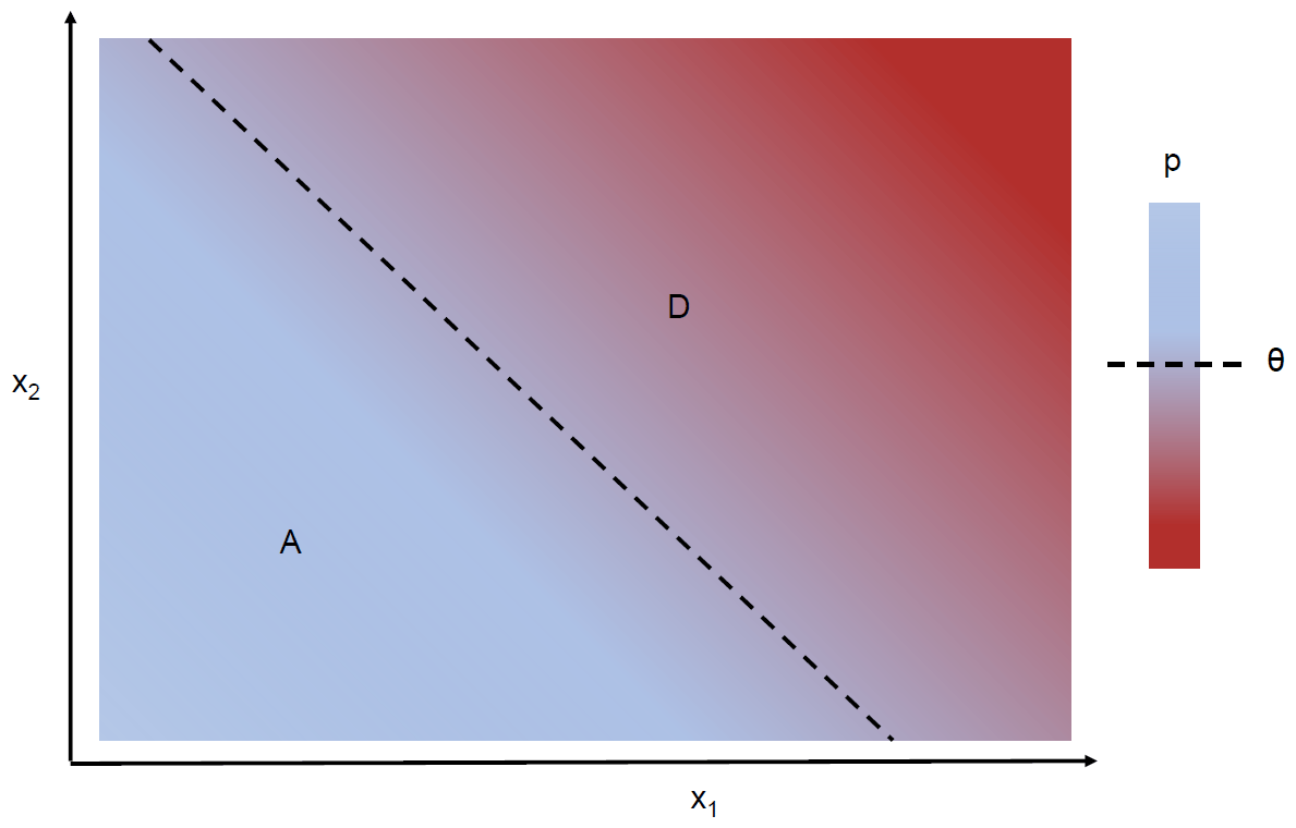
Figure 1Concept of the response surface as a stress test with descriptive variables (x1, x2). Acceptable and unacceptable regions are defined by a threshold θ over performance R.
The descriptive variables or stressors, like the mean flow, the peak flow, or temporal autocorrelations, are aggregations of the time series that are the inputs of a water system model. Because a limited number of descriptors do not capture all possible fluctuations of a time series, a term of irreducible uncertainty remains. The response surface, R, is then given by the following:
In a risk-averse approach, the objective is to find the range of unacceptable outcomes, i.e., the space over which a system fails to satisfy an acceptability threshold θ. With two variables, this space is the set of solutions to the inequality R<θ, so that, in the following:
Simplifying the response surface by, e.g., its average estimate can, thus, underestimate the unacceptability domain. The irreducible uncertainty can be addressed through adaptive management (Brown et al., 2011), but there is interest in integrating estimates of uncertainty into the response surface tool. Kay et al. (2014) proposed the use of uncertainty allowances that could vary depending on the response type and catchment. More specifically, flood control systems operate on shorter timescales and are harder to assess over long-term climate shifts (Knighton et al., 2017), increasing uncertainty in flood response functions. Kim et al. (2018) show how the choice of a longer modelling timescale (daily vs. hourly) can lead to risk underestimation. The choice of the weather generator used to generate synthetic weather series in a scenario-neutral experiment can also lead to different results (Keller et al., 2019; Nazemi et al., 2020). Steinschneider et al. (2015) and Whateley and Brown (2016) compare different sources of uncertainty in the response. Taner et al. (2019) integrate probability estimates through a Bayesian belief network model. Recently, logistic regression has been a convenient way to divide the exposure space based on probability of success (Quinn et al., 2018; Kim et al., 2019; Lamontagne et al., 2019; Hadjimichael et al., 2020; Marcos-Garcia et al., 2020).
2.1.2 Fuzzy acceptability thresholds
The acceptability criterion based on a threshold θ defines the set of acceptable outcomes. It is a subjective or arbitrary opinion from stakeholders or decision-makers to attribute a normative value to a certain performance level. The vast majority of the studies reported in the literature assume that the threshold between satisfactory and unsatisfactory outcomes is crisp (Brown et al., 2012; Culley et al., 2016; Kim et al., 2019). As such, a threshold shapes directly the partition of the response function; with a crisp value the exposure space can be subdivided in only two sub-spaces: acceptable versus unacceptable.
The very existence of a threshold is the basis of satisficing behaviors (Simon, 1955) that differ from utility maximizing behaviors, as coined by Von Neumann and Morgenstern (1944). In practice, however, there might be situations whereby the water manager is unable (or unwilling) to provide a crisp, well-defined threshold or when such threshold is disagreed upon by stakeholders. For example, when controlling water levels in a reservoir to prevent floods, the operator can handle certain tolerances above the maximum desired level. Of course, the greater the deviation from the desired level, the less acceptable it becomes.
Mathematically, fuzzy sets theory handles imprecisely defined or ambiguous quantities. Introduced by Zadeh (1965), fuzzy sets theory has become a common tool in decision-making analysis or computational sciences when nonprobabilistic, imperfect knowledge stemming from ambiguity or vagueness must be considered (Yu, 2002). In our case, fuzzy sets theory allows us to introduce vagueness in target-based decision-making, without forsaking a target-based model in favor of an unbounded maximizing behavior (although a fuzzy target can also be seen as a generalization of both maximizing and satisficing behaviors; see Castagnoli and Li Calzi, 1996, and Huynh et al., 2007).
We consider here the case where such a threshold θ may not be precisely defined by stakeholders but can take many subjective qualifications from acceptable to unbearable, hence relaxing (without fully removing) the arbitrary condition of satisfying a crisp value. A fuzzy set Aμ of acceptable states therefore qualifies the performance R with a membership value comprised between 0 and 1. The membership function μ associated to the fuzzy set A describes the degree to which any value of R more or less belongs to A (Fig. 2; Eq. 3).
When a threshold corresponds to a fuzzy set, it means that there is a transition zone between acceptable and unacceptable outcomes where intermediate levels of membership exist. Conversely, another interpretation is that the membership function is the distribution of the possibilities (Zadeh, 1978; Dubois and Prade, 1988) that any given performance R represents an acceptable outcome.
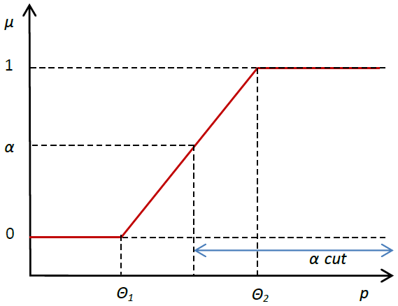
An α-cut Aα is the crisp set over Aμ for which the membership degree to Aμ is equal to or above α. The largest α-cut is called the support of the fuzzy set Aμ (R≥θ1). The smallest α-cut is the core of the fuzzy set (R≥θ2).
A fuzzy definition of acceptability is not only a way to accommodate ambiguity as a stakeholder-based constraint, but it can also alter the outcome of the analysis. Theoretically, it can happen when the slope of a response as a function of stressors is different for the compared alternatives (infrastructure investments, management rules, etc.), as illustrated in Fig. 3 for a single stressor variable. Rule 2 has a larger acceptable region with a crisp threshold, but the result is mixed with a fuzzy definition of acceptability. In that case, a trade-off appears between minimizing a loss of any sort (i.e., any type of flooding) and minimizing the maximum loss (min–max).
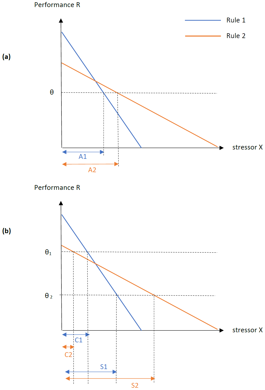
Figure 3The case of different performance slopes, as a function of a single stressor X. (a) With a crisp threshold θ, Rule 2 has a larger acceptable region A2. (b) With a fuzzy threshold (θ1, θ2), the fuzzy set of acceptable outcomes over performance R has a core (R≥θ1, where acceptability is μ=1) and a support (R≥θ2, where μ≥0), to which respective regions C and S are associated. Rule 2 has a larger domain S2 where acceptability is at least partial but a smaller full acceptability domain C2 than Rule 1.
For example, in Quinn et al. (2017a), an attempt at minimizing expected flood damage leads to worse results under extreme events most of the time. Hadjimichael et al. (2020) perform a sensitivity analysis on binary acceptability thresholds and show the impact such a definition has on the outcome of a vulnerability assessment. Criterion ambiguity could lead to similar effects, i.e., the preferred option might not be the same, depending on the value of the threshold, and in the present study it depends on the degree of acceptability.
2.2 Combination of fuzzy thresholds and uncertain response function
When incorporating a fuzzy threshold, the challenge is to combine two different sources of imperfect knowledge (described in Sect. 2.1), the uncertainty of the response itself, relative to the variables that describe change, and the ambiguity of the acceptability threshold. An approximated fuzzy random logistic regression is proposed in order to integrate both.
As the goal of the response surface is to divide the exposure space between acceptable and unacceptable outcomes, the value associated to any combination of variables can be either 0 or 1 whether a specific acceptability threshold θ is reached or not. As seen in Sect. 2.1, an intrinsic uncertainty remains in response surfaces. Several studies use a logistic regression to divide the exposure space based on probability of acceptability (Quinn et al., 2018; Kim et al., 2019; Lamontagne et al., 2019; Hadjimichael et al., 2020; Marcos-Garcia et al., 2020). The logistic regression is used to explain a binary outcome from independent variables (x1, x2) and returns a probability of acceptable outcome π as follows:
where xi are the defining variables of the exposure space, and βi are the regression coefficients. The logistic response surface therefore provides the probability π of meeting the threshold θ over the (x1, x2) exposure space. The logistic regression also has its own uncertainty, but it is not considered here. While the response surface considers a range of states of the world without knowing their probability of occurrence, the logistic regression still provides a conditional probability of acceptable outcome once a given state of the world is reached. Partitions of the space between acceptable and unacceptable subspaces that can be defined as π-cuts are now relative to a specific probability of acceptable outcome π*, taken by πθ, as follows:
By considering the domain of acceptable outcomes as a fuzzy set, we introduce a quantification of ambiguity that is different in nature from the irreducible hydroclimatic uncertainty. While the logistic regression returns a probability of surpassing any given acceptability threshold for a combination of variables (Eqs. 5 and 6), the fuzzy set of acceptable outcomes returns the possibility of any such performance value being actually considered as acceptable (Eq. 7).
Fuzzy regression models, including fuzzy logistic regression (e.g., Pourahmad et al., 2011; Namdari et al., 2013), replace probabilities by fuzzy numbers; they usually do not combine them. Fuzzy probabilities (Zadeh, 1984) are considered within the so-called fuzzy random regression field; however, no fuzzy random logistic regression seems to have been developed to date (see Chukhrova and Johannssen, 2019, for a review of the fuzzy regression field).
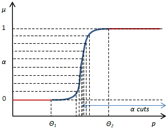
Here we use a discretized approximation of a fuzzy random logistic regression based on α-cuts. As illustrated in Figs. 2 and 4, a fuzzy set Aμ can be decomposed in α-cuts. Each α-cut is a crisp set, and the values belonging to an α-cut also belong to the fuzzy set Aμ with a membership degree equal to or above α.
Therefore, any crisp set of acceptable outcomes A, defined by a single threshold θ, is also an α-cut of the fuzzy set of acceptable outcomes Aμ. Then, a single logistic regression for any acceptability threshold θ is also the probability of belonging to the α-cut of the fuzzy set of acceptable outcomes defined by θ as follows:
with α=μ(θ).
Following the interpretation of Huynh et al. (2007), the overall possibility Π of the random variable R belonging to the fuzzy set Aμ can be given by the integral over α of the probabilities of acceptability defined at every α-cut.
And, thus,
The approximated logistic regression for a fuzzy set of acceptable outcomes is, therefore, the average of the logistic regressions for all the associated α-cuts. With a uniform discretization of 10 α levels, the spacing of every α-cut, defined with , relies on the shape of the membership function. A linear shape of μ(R) leads to a uniform sampling of the α-cuts, while a sigmoid error function leads to a Gaussian sampling of α-cuts centered on (Fig. 4).
A two-reservoir system in eastern Canada is used as a case study to illustrate the applicability of the possibilistic response surfaces.
3.1 Upper Saint François River basin features
The Upper Saint François River basin (USFRB) is located in the province of Quebec, Canada. The selected gauging point, near the agglomeration of Weedon, drains an area of 2940 km2 with an average annual flow of 2.1 ×10⁷ m3. The system (Fig. 5) involves the Saint François River, controlled by two reservoirs (Great Lake Saint François and Lake Aylmer) with a combined storage capacity of 941 ×106 m3 and the uncontrolled affluent Saumon River.
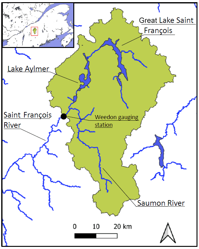
Figure 5Layout of the Upper Saint François River basin, Quebec, Canada. (Map credit: Ministère de l'Environnement et de la Lutte contre les changements climatiques.)
Both reservoirs are managed by the Quebec Water Agency, which is part of the Ministry of Environment (Ministère de l'Environnement et de la Lutte contre les changements climatiques – MELCC). The main operational objectives are (i) to protect the municipality of Weedon and several residential areas around the lakes from floods, (ii) to ensure minimum river discharges and water levels in the lakes to preserve aquatic ecosystems, (iii) to regulate the floods for downstream power plants, and (iv) to maintain desired water levels in the lakes for recreational use during the summer (Fortin et al., 2007).
This multipurpose reservoir system thus follows a refill–drawdown cycle accordingly. With a snowmelt-dominated flow regime, the reservoirs are emptied in winter, filled during the spring, and kept at a constant pool elevation during the summer.
3.2 Inflow time series
At the request of the system operators, we use hydrologic stressors instead of climatic ones. Other authors have also used hydrologic stressors (see, e.g., Nazemi et al., 2013, 2020; Borgomeo et al., 2015; Herman et al., 2014). Readily available inflow time series from GCM weather projections are used to generate additional synthetic streamflow series, as in Vormoor et al. (2017). Results are then directly plotted on the exposure space according to their own (x1, x2) coordinates. Such a method seeks to make greater use of hydroclimatic future scenarios when many are already available and to obtain a higher diversity of synthetic times series (based on different GCM simulations, Representative Concentration Pathway (RCP) scenarios, and downscaling techniques). We first describe the initially available time series and then how they are perturbed and reused to create synthetic time series.
Historical daily measurements are available for the 2000–2014 period (MELCC, 2018). They include the lakes' inflows, levels, and reservoir releases and river discharges from the tributary and at the basin outlet.
Streamflow scenarios are provided by MELCC through the Quebec Water Atlas 2015 (CEHQ, 2015; MELCC, 2018). Those hydrologic projections are based on climatic projections from the Natural Resources Canada database of GCM simulations (CMIP5; CEHQ, 2015). Meteorological time series were bias corrected by the Quebec Water Agency for the reference climate (1971–2000 period) and then processed by the HYDROTEL model (Fortin et al., 2001) for all major rivers in the southern part of the Quebec province. For the Upper Saint François River basin, resulting hydrological simulations were also bias corrected with the historical flow record and the quantile mapping approach.
A set of 501 time series was made available, spanning 30 years of daily inflows. The set contains 135 scenarios for a 1971–2000 reference period and 366 scenarios for the 2041–2070 period. The 366 scenarios are based on 122 GCM projections to which three different downscaling techniques were applied, i.e., projections without bias correction, with quantile mapping, or with delta quantile mapping (based on Mpelasoka and Chiew, 2009). In order to obtain the largest degree of variability, and find as many failure configurations as possible, all 501 time series are used indistinctively. These runoff time series are first perturbed to increase the sample size and cover a wider share of the exposure space and are then used as input for the synthetic time series generation.
In order to expand the sample of the exposure space and explore less favorable conditions, the perturbation of available inflows is performed by either modifying the average annual flow, the dispersion of daily flows, or both. To increase the range of tested inflow volumes, a single change factor is applied in the first case, arbitrarily increasing all flow values at every time step by 50 %. To perturb the dispersion, a varying factor multiplies flow values, depending on their rank in the series distribution (factor 1 for the lowest flow and factor 1.5 for the highest flow). There are then four categories of perturbation, namely volume only, dispersion, volume and dispersion, and none.
This expanded set of time series is then used as the input of the synthetic generator. The generator is the Kirsch–Nowak method (Nowak et al., 2010; Kirsch et al., 2013), made available online as MATLAB code by Quinn et al. (2017b), as employed, e.g., in Quinn et al. (2017a). Each synthetic generation is performed twice for each available time series. We then obtain 501 (initial tie series) × 4 (different perturbations) × 2 (synthetic realizations) = 4008 synthetic time series, each containing 30 years of daily river discharges.
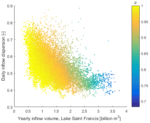
Similar to other stress test studies that generate inflow instead of climate time series (Feng et al., 2017), the selected driving variables (axes x and y of the response function) are the total annual inflow volume and a measure of the intra-annual variability in streamflow. The intra-annual variability is here measured with the dispersion coefficient G, a measure also known as Gini coefficient in economics but employed in hydrology too (Masaki et al., 2014). It is similar to the coefficient of variation used in, e.g., Nazemi et al. (2020) but bound between 0 and 1, which offers the following convenient interpretation: at G=0 all daily discharges in a year are equal; if G=1, the entire yearly runoff happens in a single day. Like the variation coefficient, it allows for a second variable statistically independent of the total annual runoff volume. Here qi are the ordered daily discharges of a given year, i.e., N=365 d.
3.3 Simulation and response surface
The model is built with HEC-ResSim, the Reservoir System Simulation software developed by the U.S. Army Corps of Engineers (Klipsch and Hurst, 2007). It relies on a network of elements representing the physical system (reservoirs, junctions, and routing reaches) and the sets of operating rules. HEC-ResSim replicates the decision-making process applied to many actual reservoirs through a rule-based modeling of operational constraints and targets.
Hydrologic inputs consist of 30-year-long daily river discharges for each sub-basin. The main outputs are daily water levels in lakes, reservoir releases, and the discharges at the outlet. A complementary Jython routine is developed in order to run HEC-ResSim in a loop to systematically load a large set of different hydroclimatic scenarios. Dam characteristics and operational rules were provided by the Quebec Water Agency (MELCC, 2018).
The model is developed with a first set of operating rules (Rule 1) expected to mimic the current operation of the system. It reproduces measured daily releases over the 2000–2014 period. A total of 4008 simulations are then run, each taking an input of synthetic daily flow series spanning 30 years. In order to increase the density of the ungridded exposure space sampling, the results are divided into 5-year periods. Such a decomposition is deemed acceptable based on the reservoir system, whose storage capacity is designed for seasonal, not multiyear, regulation, mitigating the effects of boundary conditions. It leads to a sample of 24 048 points, with each one representing a 5-year simulation.
Although the operating rules were designed by taking all operating objectives into account, the present study focuses on the flood control performance R. More specifically, it is the reliability (Hashimoto et al., 1982; Loucks and van Beek, 2017) of the system keeping the river discharge at Weedon below 300 m3 s−1. Mathematically, if F(t) is the state of flooding at time step t, then R is given by the following:
The response function is built by representing performance R as a function of the selected inflow characteristics (yearly volume and dispersion). We consider the case where the threshold between acceptable and unacceptable performance is not clearly defined but is bounded between θ1=0.93 and θ2=0.97.
The separation of the exposure space between acceptable and unacceptable regions is calculated following Sect. 2, combining a logistic regression with a fuzzy acceptability domain, with its support being [0.93, 1] and its core [0.97, 1]. Consequently, any given performance value R has a membership degree of 0 for R<0.93 and is equal to 1 for R≥0.97. A counterfactual exercise is also run with a crisp threshold , where the ambiguity is ignored and only the median between bounds is selected. Performance is also calculated for a sub-set of GCM-based projections deemed more trustworthy by the Centre d'expertise hydrique du Québec (CEHQ; with quantile mapping downscaling for the 2041–2070 period), with each one divided into 5-year periods.
These rules are compared to an instrumental set (Rule 2), which slightly alters the anticipation and emergency release algorithm of the reservoirs.
The simulation is first run with 122 of the original time series made available by the Quebec Water Agency. These are the bias-corrected rainfall–runoff simulations considered as being the most reliable for scenario-driven adaptation plans and corresponding to different radiative forcing scenarios. Taken in 5-year periods (thus, 610 time series), the values all lead to flood control reliabilities superior to 0.97, which is above any considered acceptability threshold. So, both rule sets are considered successful in all these time series.
Simulations are then run for the much larger and more diverse sample of 4008 synthetic time series. The performance R, measured as the reliability of flood control, is evaluated for each 5-year period contained in the 4008 simulations of 30 years (24 048 evaluations). The color scale represents the performance (reliability R against floods) in Fig. 6 for each 5-year time series. The axes are the stressors x1, x2, showing the average annual inflow volume at Great Lake Saint François and the dispersion (or Gini coefficient) of the daily inflows. The response shows considerable noise, although a northeast–southwest anisotropy or gradient can be visually noticed.
An acceptability value μ is then associated to each dot (time series) in the sample, depending on the value of the performance (reliability) R (Fig. 7a). The acceptability value μ is the membership degree of R to the fuzzy set of acceptable outcomes, with [0.93, 1] as the support and [0.97, 1] as the core (as in Fig. 2). The sample of simulations, thus, leads to acceptability values between 0 and 1 in Fig. 7a.
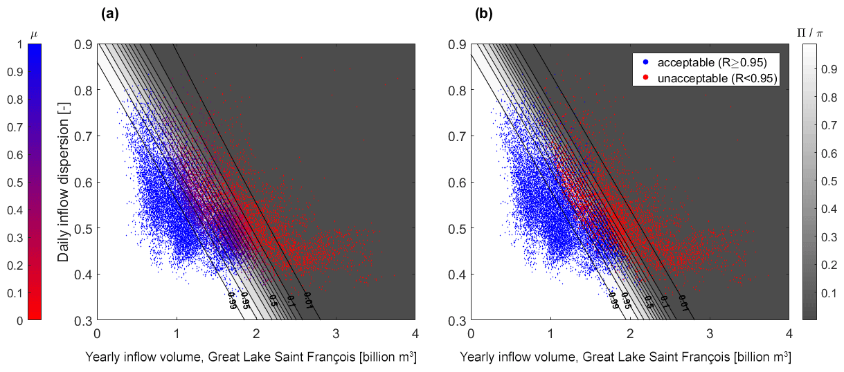
Figure 7Acceptability of sampled outcomes and logistic regressions. (a) Fuzzy outcomes and the possibility of an acceptable performance Π. (b) Binary outcomes and the probability of an acceptable performance π.
To solve the problem of combining two uncertainties that are different in nature (the probability of meeting a threshold vs. the possibility that this threshold is acceptable), the aggregated logistic regression presented in Sect. 2.2.1 is performed for the fuzzy outcomes, thus proposing a continuous mapping for a case where the outcomes are not available as binary categories. The logistic regression is performed 10 times for 10 α-cuts corresponding to a uniform sampling of α levels. The aggregated logistic regression at every coordinate is the average of the 10 logistic regressions, with each one considering a single α-cut as being the crisp set over R that defines acceptable outcomes.
It provides, at each coordinate of the exposure space (or state of the world), a possibility value Π of the outcome (reliability against floods) deemed as being acceptable given the realization of the state of the world. This – conditional – possibility measure expresses both the ambiguity of the acceptability criterion and the probability of an acceptable outcome at any location on the response surface. The surface can be divided into acceptable and unacceptable regions (Fig. 7) based on any desired level of possibility (Π-cut).
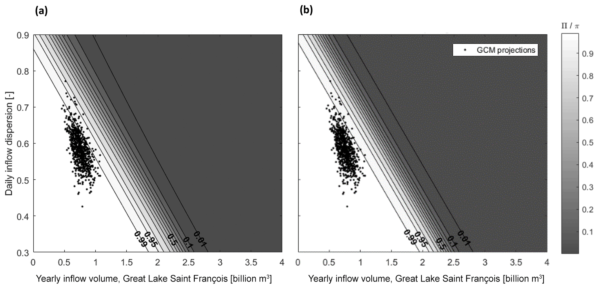
Figure 8Logistic regressions and GCM projections (a) for fuzzy outcomes and (b) for binary outcomes.
As a counterfactual point, we also compute an alternative, where the ambiguity of the threshold is ignored with the response surface converted into binary outcomes – acceptable or unacceptable frequency of flooding – based on a median crisp threshold of 0.95 (Fig. 7b). A simple logistic regression is performed for the counterfactual binary outcomes, leading to a probability π of acceptable outcome.
The approximation was done with the MATLAB® function mnrfit. The McFadden pseudo R2 of the median threshold logistic regression is 0.7531. The relation between explanatory variables is kept linear, as introducing an interaction term only increased the pseudo R2 to 0.7562. These values are considered as being an acceptable goodness of fit for this study. A pseudo R2 equal to 1 represents a perfect model, and a value of 0 means that the logistic model is not a better predictor of probabilities than an intercept-only model. A possible room for improvement of the predicting value of the model would be to change the predictors, although it was not the core of this study. Selecting two different predictors from a larger set of candidates might increase the final R2 (by performing a first round of logistic regressions for each pair and selecting the pair with highest R2, as in Quinn et al., 2018).
Π-cuts producing frontiers between acceptability regions can be contrasted with the mapping of the time series from GCM projections on the response surface (Fig. 8). While all these downscaled time series lead to fully acceptable performances, showing reliability values above 0.97, their coordinates, and thus their corresponding state of the world, can still fall below a Π-cut.
This is because, for any of these projections, the evaluated sequence is one realization of those conditions x1, x2. Assuming that the logistic regression model is accurate with the possibility of 1-Π, alternative realizations of those conditions may not be seen as being satisfactory. A scenario sharing the same properties x1, x2, i.e., yearly inflow volume and daily inflow dispersion, with a satisfactory GCM projection could still lead to an unacceptable frequency of flooding if its possibility of acceptable outcome Π is below the acceptable level.
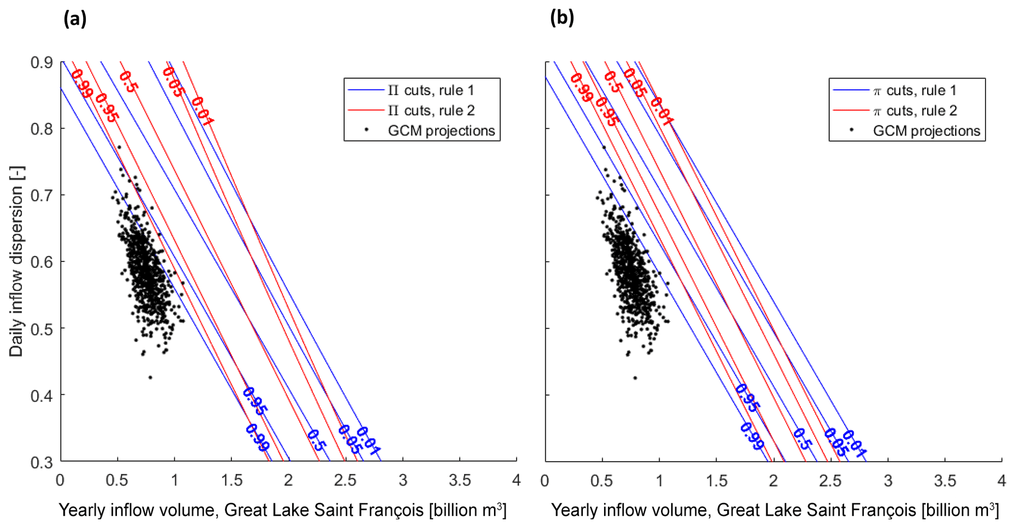
Figure 9Compared logistic regressions, Rules 1 and 2, and GCM projections for (a) fuzzy outcomes and (b) binary outcomes.
Respectively, the binary counterfactual model (Fig. 8b), provides a degree of probability π of an unacceptable outcome for the same state of the world as in the previous studies using the logistic regression. Figure 8 illustrates the straightforward difference between adapting to the ambiguity of the acceptability criterion (Fig. 8a) and ignoring it (Fig. 8b). For any given state of the world (coordinate) x1, x2, the aggregated logistic regression not only considers the probability of a realization leading to a certain performance, but also the possibility that such performance, the reliability against floods, would be considered an acceptable outcome. Accepting a fuzzy acceptability criterion thus mechanically widens the range of the continuous transition resulting from the logistic regressions. A state of the world with a near 100 % probability of meeting a 0.95 reliability threshold might still have a possibility of this threshold not actually being accepted.
Such differences are more noticeable in this case study when using GCM projections as ex post weights. With a fuzzy target, 46 projections (6.3 %) fall out of the 0.99 Π-cut, i.e., the sub-space where the possibility of acceptable outcome is at least 0.99. Said otherwise, there is a possibility of at least 0.01 that a realization leading to the same state of the world (coordinates) would produce a flooding pattern considered as being unacceptable according to the aggregated logistic regression. With a crisp simplification, thus with less information, 17 projections (2.3 %) fall out of the 0.99 π-cut. There is a probability of at least 0.01 that a realization leading to the same state of the world would produce an unacceptable outcome.
These frontiers are specific to a reservoir operation rule. When using a stress test with a response surface, alternative rules are compared based on the relative position of the frontiers between acceptable and unacceptable regions. Altogether, two of them are compared, namely an approximation of current reservoir operations (Rule 1) and an alternative, instrumental set of rules (Rule 2). Figure 9 compares the two rules based on selected Π-cuts (Fig. 9a). The counterfactual calculation with binary outcomes and π-cuts is also provided (Fig. 9b).
Figure 9 shows a situation partially similar to the theoretical situation of Fig. 2, where the relative advantage of each rule depends on the location on the exposure space and the preferred level of possibility. With a fuzzy acceptability criterion (Fig. 9a), Rule 2 is preferred to Rule 1 for the high possibility of an acceptable outcome (Π≥0.95) because the region defined by this frontier for Rule 2 is larger than for Rule 1. It means that Rule 2 leads to acceptable outcomes in a larger range of states of the world than Rule 1. However, for low possibilities of an acceptable outcome (below 0.05), the comparison depends on the stressors x1, x2. Rule 2 is preferred for very high daily inflow dispersion (or Gini coefficient; y axis) but moderate yearly inflow (x axis), while Rule 1 is preferred for low dispersion and very high yearly inflows (again assuming the logistic regression model is accurate).
Using a counterfactual with binary outcomes (Fig. 9b), and thus frontiers defined only by probabilities, modifies the above results. While Rule 2 remains preferable for high probabilities of acceptable outcomes, it becomes worse than Rule 1 for low probability cuts, which is this time independent of the location on the exposure space.
If the decision-makers choose to use GCM projections as ex post weights, the preference order for low possibility levels becomes less important. It narrows the relevance of the exposure space to the vicinity of the projections and, thus, to the high possibilities of acceptable outcomes. In this case, eight scenarios for Rule 2 (1.1 %) fall below the 0.99 Π-cut (meaning that other realizations have a 0.01 possibility of unacceptable outcome) compared to 46 scenarios for Rule 1 (6.3 %). Again, all GCM-based scenarios lead to fully acceptable outcomes (R≥0.97). Rule 2 would then be preferred to Rule 1, but there would still be a possibility of unacceptable outcome superior to 0.01 with this rule for the same states of the world (coordinates x1, x2) sampled by the GCM-based scenarios.
Using only binary outcomes, thus only probability-based frontiers, produces a slightly different result. Rule 2 is not only preferred in the vicinity of the GCM projections but also no such projection falls below the 0.99 π-cut. The probability of unacceptable outcome is, thus, less than 0.01 at the vicinity of any GCM projection. Based on such projections, Rule 2 would be adopted with less reservations with a binary model than with a fuzzy model.
By itself, a stress test approach can be seen as a departure from a probabilistic framework towards a possibilistic one. The stress test of a water system, through a response surface, asks which states of the world could possibly lead to an unacceptable outcome instead of evaluating the system performance with a given probability.
In this paper, we consider that the threshold employed to define acceptable outcomes might be ambiguous or contentious. The fuzzy or possibilistic framework (Zadeh, 1965, 1978; Dubois and Prade, 1988), often used in decision-making analysis, provides the analytical tools to incorporate an uncertainty that is not probabilistic, the ambiguity of a decision threshold, within the increasingly popular stress test tool.
Applying a fuzzy threshold would be straightforward for a deterministic response surface, with each performance value on the exposure space being mapped to a degree of acceptability between 0 and 1. This study explores how to solve the problem of combining a fuzzy definition of acceptability with the remaining hydroclimatic uncertainty of the response surface itself. These two concepts represent the following different sources of imperfect knowledge: one applies to the performance of the system and the other to the qualification of this performance as being acceptable or not. To integrate them in a same response surface, the methodology relies on the concept of α-cuts to produce an aggregated logistic regression from a membership function.
The case study of the Upper Saint François reservoir system illustrates the implementation of the aggregated logistic regression and the conceptual framework behind it. Just like for previous uses of logistic regression, in the present method, the response surface does not show a single frontier that divides the exposure space between acceptable and unacceptable flooding outcomes but rather a parametric frontier depending, in this case, on a desired level of possibility. While possibility and probability levels cannot be directly compared (the first comprises the latter), their difference is illustrated by the wider spread of the transition zone in the response functions. This wider spread is to be expected as more sources of ambiguity are considered in the possibilistic approach, and a consequence can be that GCM projections may fall below an acceptability frontier when they do not for a probabilistic logistic regression.
Although the main goal of this study is to propose a practical adaptation to a stakeholder-driven constraint (the absence of a clear threshold), results also explore the effect that threshold ambiguity can have on final decisions. Compared response surfaces show that ignoring the ambiguity of a criterion can alter the comparison between options, which is either based on the size of the acceptable domains or on the position of GCM projections in the response surface. While specifically applying this criterion for a fuzzy approach with varying degrees of acceptability, this type of result is comparable to more general sensitivity studies over binary thresholds, as in Hadjimichael et al. (2020). Not accounting for the criterion ambiguity may, thus, lead, in some cases and for some actors, to floods perceived as being worse with the selected option than with the discarded option.
Results show that the preference between options can change depending on the possibility level Π. When this happens, selecting the appropriate level Π threshold is highly consequential and depends on the involved actors. This challenge is the equivalent, in possibilistic terms, to the selection of the probability threshold π in the non-fuzzy logistic regression (Kim et al., 2019). The π threshold depends on both a probability level and the value of α.
Defining the membership function μ does introduce an additional layer of complexity in the modelling process. It is ultimately up to the modeler and stakeholders to decide if it is a necessary translation of the social reality, while keeping in mind how it can affect the results. The elaboration of membership functions from linguistic information has been well studied in many fields (Zimmermann, 2001; Garibaldi and John, 2003; Sadollah, 2018), including in water resources management (Khazaeni et al., 2012). Future works should further explore how to elaborate adapted membership functions specific to the linguistic inputs that characterize satisfaction thresholds in the case of flood control systems.
To further address both challenges of selecting the appropriate possibility level Π and eliciting the membership function μ, loss aversion, as developed by Kahneman and Tversky (1979) in prospect theory, would also be a useful concept. A parallel can be drawn with Quinn et al. (2018), where the choice of the probability level π in a logistic regression is instead linked to risk aversion.
Other studies have linked prospect theory with membership functions for fuzzy sets (e.g., Liu et al., 2014; Andrade et al., 2014; Gu et al., 2020). While this study focuses on the practical integration of ambiguity as a real-world constraint, further theoretical research should focus on linking both risk and loss attitudes to hydroclimatic response functions.
An important caveat is that the response surface relies on a specific set of realizations from a synthetic generator and a starting data set that is perturbed and reshuffled. The choices and assumptions that lead to a realization deserve further scrutiny in future works. Ungridded, on-the-fly sampling here allows us to more freely explore the variability in the response, as the focus of the study is the diversity of outcomes for a given coordinate. The sampling should be improved to cover the exposure space more evenly but without constraining too much the diversity of time series. The impact of the choice of a given synthetic generator, of the sample size, and of the perturbation process should be further examined. Likewise, the choice of describing variables was not the focus of the study but should be subject to an initial comparison among a larger number of candidate predictors. Finally, the quality of the logistic model should be further analyzed. External validation with a separate sampling of the exposure space should be included (Kim et al., 2019). Further work should seek to integrate the goodness of fit and the external validation as additional sources of uncertainty within the method. All the aforementioned steps should be considered for this possibilistic method to be used as policy recommendation.
A possibilistic framework could integrate within a response surface many more of these kinds of uncertainties when probabilities are not relevant or too uncertain, as done in other water management studies (El-Baroudy and Simonovic, 2004; Afshar et al., 2011; Jun et al., 2013; Le Cozannet et al., 2017; Qiu et al., 2018; Wang et al., 2021). One particularly suitable use of fuzzy logic should be to consider as fuzzy values the ex post expert judgment on the possibility or likeliness of the obtained synthetic time series in a given river basin. The synthetic generator explores time series configurations, but those may not always correspond to the range of outcomes expected in a watershed.
The integration of the uncertainty and ambiguity quantification within the response surface tool could allow for aggregation options in a multi-objective problem (like in Poff et al., 2016; Kim et al., 2019), while easily controlling its two separate components, i.e., response uncertainty and threshold ambiguity.
Importantly, the response surface is here considered as being a generic tool for decision-making under deep uncertainty, but it is used within more complex frameworks. Further research should also analyze how fuzzy thresholds can be inserted within a more complete set of methods.
We explore, in this study, how to integrate ambiguous acceptability thresholds within uncertain response surfaces in decision-centric vulnerability assessments. We propose a method to produce a possibilistic surface when the fuzzy threshold is applied to an uncertain surface. Aggregating logistic regressions over α-cuts incorporates, in a single measure, the ambiguity of the acceptability threshold and the probability of meeting such threshold for a given state of the world. The method is illustrated with the Upper Saint François reservoir system in Canada. We show how a fuzzy threshold shapes the response surface and how the way this ambiguity is treated can affect the vulnerability assessment.
Challenging old probabilistic assumptions, notably in a climate crisis context, brings new tools that also imply new choices and degrees of arbitrariness. How to transparently elaborate fuzzy thresholds jointly with stakeholders, or the choice of a synthetic scenario generator, are necessary research continuations. The presented approach can be followed by further work on stakeholder attitudes, multi-objective problems, and aggregation choices in bottom-up vulnerability assessments. The framework introduced here to solve a practical challenge can be consolidated from a more theoretical perspective, from both possibility theory and decision-making, under deep uncertainty.
The data can be provided upon authorization from MELCC, Quebec, Canada (Ministère de l'Environnement et de la Lutte contre les Changements Climatiques). The codes required to reproduce the results are available upon request (thibaut.lachaut1@ulaval.ca).
TL and AT conceptualized the study. TL developed the methods, models, and simulations and drafted the paper. AT acquired the funding and provided extensive supervision.
The contact author has declared that neither they nor their co-author has any competing interests.
Publisher's note: Copernicus Publications remains neutral with regard to jurisdictional claims in published maps and institutional affiliations. This study does not represent the views of MELCC.
The authors would like to thank Louis-Guillaume Fortin, Richard Turcotte, and Julie Lafleur from the CEHQ, for the fruitful discussions and the knowledge of the reservoir system, Alexandre Mercille and Xavier Faucher, who contributed to earlier versions of the HEC-ResSim model, and Jean-Philippe Marceau, who developed the iterative Jython routine.
The work was supported by a project from Ministère de l'Environnement et de la Lutte contre les Changements Climatiques (MELCC; Quebec, Canada) entitled “Étude visant l'adaptation de la gestion des barrages du système hydrique du Haut-Saint-François à l'impact des changements climatiques dans le cadre du Plan d'action 2013–2020 sur les changements climatiques (PACC 2020; Fonds vert)”.
This paper was edited by Ann van Griensven and reviewed by three anonymous referees.
Afshar, A., Mariño, M. A., Saadatpour, M., and Afshar, A.: Fuzzy TOPSIS Multi-Criteria Decision Analysis Applied to Karun Reservoirs System, Water Resour. Manage., 25, 545–563, https://doi.org/10.1007/s11269-010-9713-x, 2011.
Andrade, R. A. E., González, E., Fernández, E., and Gutiérrez, S. M.: A Fuzzy Approach to Prospect Theory, in: Soft Computing for Business Intelligence, in: Studies in Computational Intelligence, edited by: Espin, R., Pérez, R. B., Cobo, A., Marx, J., and Valdés, A. R., Springer, Berlin, Heidelberg, 45–66, https://doi.org/10.1007/978-3-642-53737-0_3, 2014.
Ben-Haim, Y.: Info-Gap Decision Theory: Decisions Under Severe Uncertainty, Academic Press, London, https://doi.org/10.1016/B978-0-12-373552-2.X5000-0, 2006.
Borgomeo, E., Farmer, C. L., and Hall, J. W.: Numerical rivers: A synthetic streamflow generator for water resources vulnerability assessments, Water Resour. Res., 51, 5382–5405, https://doi.org/10.1002/2014WR016827, 2015.
Broderick, C., Murphy, C., Wilby, R. L., Matthews, T., Prudhomme, C., and Adamson, M.: Using a scenario‐neutral framework to avoid potential maladaptation to future flood risk, Water Resour. Res., 55, 1079–1104, https://doi.org/10.1029/2018WR023623, 2019.
Brown, C. and Wilby, R. L.: An alternate approach to assessing climate risks, Eos Trans. Am. Geophys. Union, 93, 401–402, https://doi.org/10.1029/2012EO410001, 2012.
Brown, C., Werick, W., Leger, W., and Fay, D.: A decision-analytic approach to managing climate risks: Application to the upper Great Lakes, J. Am. Water Resour. Assoc., 47, 524–534, https://doi.org/10.1111/j.1752-1688.2011.00552.x, 2011.
Brown, C., Ghile, Y., Laverty, M., and Li, K.: Decision scaling: Linking bottom-up vulnerability analysis with climate projections in the water sector, Water Resour. Res., 48, W09537, https://doi.org/10.1029/2011WR011212, 2012.
Brown, C., Steinschneider, S., Ray, P., Wi, S., Basdekas, L., and Yates, D.: Decision Scaling (DS): decision support for climate change, in: Decision Making under Deep Uncertainty: From Theory to Practice, edited by: Marchau, V. A. W. J., Walker, W. E., Bloemen, P. J. T. M., and Popper, S. W., Springer International Publishing, Cham, 255–287, https://doi.org/10.1007/978-3-030-05252-2_12, 2019.
Castagnoli, E. and Li Calzi, M. L.: Expected utility without utility, Theor. Decis., 41, 281–301, https://doi.org/10.1007/BF00136129, 1996.
CEHQ – Centre d'Expertise Hydrique du Québec: Atlas hydroclimatique du Québec méridional – Impact des changements climatiques sur les régimes de crue, d'étiage et d'hydraulicité à l'horizon 2050, Québec, 2015.
Chukhrova, N. and Johannssen, A.: Fuzzy regression analysis: Systematic review and bibliography, Appl. Soft Comput., 84, 105708, https://doi.org/10.1016/j.asoc.2019.105708, 2019.
Culley, S., Noble, S., Yates, A., Timbs, M., Westra, S., Maier, H. R., Giuliani, M., and Castelletti, A.: A bottom-up approach to identifying the maximum operational adaptive capacity of water resource systems to a changing climate: identifying the maximum operational adaptive capacity, Water Resour. Res., 52, 6751–6768, https://doi.org/10.1002/2015WR018253, 2016.
DiFrancesco, K., Gitelman, A., and Purkey, D.: Bottom-Up Assessment of Climate Risk and the Robustness of Proposed Flood Management Strategies in the American River, CA, Water, 12, 907, https://doi.org/10.3390/w12030907, 2020.
Dubois, D. and Prade, H.: Possibility Theory: An Approach to Computerized Processing of Uncertainty, Plenum, New York, ISBN 9780306425202, 1988.
Dubois, D., Foulloy, L., Mauris, G., and Prade, H.: Probability-possibility transformations, triangular fuzzy sets, and probabilistic inequalities, Reliable Comput., 10, 273–297, https://doi.org/10.1023/B:REOM.0000032115.22510.b5, 2004.
El-Baroudy, I. and Simonovic, S. P.: Fuzzy criteria for the evaluation of water resource systems performance, Water Resour. Res., 40, W10503, https://doi.org/10.1029/2003WR002828, 2004.
Feng, M., Liu, P., Guo, S., Gui, Z., Zhang, X., Zhang, W., and Xiong, L.: Identifying changing patterns of reservoir operating rules under various inflow alteration scenarios, Adv. Water Resour., 104, 23–36, https://doi.org/10.1016/j.advwatres.2017.03.003, 2017.
Fortin, J.-P., Turcotte, R., Massicotte, S., Moussa, R., Fitzback, J., and Villeneuve, J.-P.: Distributed Watershed Model Compatible with Remote Sensing and GIS Data. I: Description of Model, J. Hydrol. Eng., 6, 91–99, https://doi.org/10.1061/(ASCE)1084-0699(2001)6:2(91), 2001.
Fortin, L.-G., Turcotte, R., Pugin, S., Cyr, J.-F., and Picard, F.: Impact des changements climatiques sur les plans de gestion des lacs Saint-François et Aylmer au sud du Québec, Can. J. Civ. Eng., 34, 934–945, https://doi.org/10.1139/l07-030, 2007.
Garibaldi, J. and John, R.: Choosing membership functions of linguistic terms, in: vol. 1, The 12th IEEE International Conference on Fuzzy Systems, FUZZ'03, 25–28 May 2003, St. Louis, MO, USA, 578–583, https://doi.org/10.1109/FUZZ.2003.1209428, 2003.
Gu, J., Zheng, Y., Tian, X., and Xu, Z.: A decision-making framework based on prospect theory with probabilistic linguistic term sets, J. Operat. Res. Soc., 72, 879–888, https://doi.org/10.1080/01605682.2019.1701957, 2020.
Hadjimichael, A., Quinn, J., Wilson, E., Reed, P., Basdekas, L., Yates, D., and Garrison, M.: Defining Robustness, Vulnerabilities, and Consequential Scenarios for Diverse Stakeholder Interests in Institutionally Complex River Basins, Earth's Future, 8, e2020EF001503, https://doi.org/10.1029/2020EF001503, 2020.
Hashimoto, T., Stedinger, J. R., and Loucks, D. P.: Reliability, resiliency, and vulnerability criteria for water resource system performance evaluation, Water Resour. Res., 18, 14–20, https://doi.org/10.1029/WR018i001p00014, 1982.
Herman, J. D., Zeff, H. B., Reed, P. M., and Characklis, G. W.: Beyond optimality: Multistakeholder robustness tradeoffs for regional water portfolio planning under deep uncertainty, Water Resour. Res., 50, 7692–7713, https://doi.org/10.1002/2014WR015338, 2014.
Huynh, V.-N., Nakamori, Y., Ryoke, M., and Ho, T.-B.: Decision making under uncertainty with fuzzy targets, Fuzzy Optimiz. Decis. Mak., 6, 255–278, https://doi.org/10.1007/s10700-007-9011-0, 2007.
Jun, K.-S., Chung, E.-S., Kim, Y.-G., and Kim, Y.: A fuzzy multi-criteria approach to flood risk vulnerability in South Korea by considering climate change impacts, Exp. Syst. Appl., 40, 1003–1013, https://doi.org/10.1016/j.eswa.2012.08.013, 2013.
Kahneman, D. and Tversky, A.: Prospect theory: an analysis of decision under risk, Econometrica, 47, 263–291, https://doi.org/10.2307/1914185, 1979.
Kay, A. L., Crooks, S. M., and Reynard, N. S.: Using response surfaces to estimate impacts of climate change on flood peaks: assessment of uncertainty, Hydrol. Process., 28, 5273–5287, https://doi.org/10.1002/hyp.10000, 2014.
Keller, L., Rössler, O., Martius, O., and Weingartner, R.: Comparison of scenario‐neutral approaches for estimation of climate change impacts on flood characteristics, Hydrol. Process., 33, 535–550, https://doi.org/10.1002/hyp.13341, 2019.
Khazaeni, G., Khanzadi, M., and Afshar, A.: Fuzzy adaptive decision making model for selection balanced risk allocation, Int. J. Project Manage., 30, 511–522, https://doi.org/10.1016/j.ijproman.2011.10.003, 2012.
Kim, D., Chun, J. A., and Aikins, C. M.: An hourly-scale scenario-neutral flood risk assessment in a mesoscale catchment under climate change, Hydrol. Process., 32, 3416–3430, https://doi.org/10.1002/hyp.13273, 2018.
Kim, D., Chun, J. A., and Choi, S. J.: Incorporating the logistic regression into a decision-centric assessment of climate change impacts on a complex river system, Hydrol. Earth Syst. Sci., 23, 1145–1162, https://doi.org/10.5194/hess-23-1145-2019, 2019.
Kirsch, B. R., Characklis, G. W., and Zeff, H. B.: Evaluating the impact of alternative hydro-climate scenarios on transfer agreements: practical improvement for generating synthetic streamflows, J. Water Resour. Pl. Manage., 139, 396–406, https://doi.org/10.1061/(ASCE)WR.1943-5452.0000287, 2013.
Klipsch, J. and Hurst, M.: HEC-ResSim: reservoir system simulation, User's manual version 3.0 CPD-82, USACE, Hydrologic Engineering Center, Davis, CA, 2007.
Knighton, J., Steinschneider, S., and Walter, M. T.: A vulnerability-based, bottom-up assessment of future riverine flood risk using a modified peaks-over-threshold approach and a physically based hydrologic model, Water Resour. Res., 53, 10043–10064, https://doi.org/10.1002/2017WR021036, 2017.
Lamontagne, J. R., Reed, P. M., Marangoni, G., Keller, K., and Garner, G. G.: Robust abatement pathways to tolerable climate futures require immediate global action, Nat. Clim. Change, 9, 290–294, https://doi.org/10.1038/s41558-019-0426-8, 2019.
Le Cozannet, G., Manceau, J.-C., and Rohmer, J.: Bounding probabilistic sea-level projections within the framework of the possibility theory, Environ. Res. Lett., 12, 014012, https://doi.org/10.1088/1748-9326/aa5528, 2017.
Lempert, R. J.: Robust Decision Making (RDM), in: Decision Making under Deep Uncertainty: From Theory to Practice, edited by: Marchau, V. A. W. J., Walker, W. E., Bloemen, P. J. T. M., and Popper, S. W., Springer International Publishing, Cham, 23–51, https://doi.org/10.1007/978-3-030-05252-2_2, 2019.
Lempert, R. J., Groves, D. G., Popper, S. W., and Bankes, S. C.: A general, analytic method for generating robust strategies and narrative scenarios, Manage. Sci., 52, 514–528, https://doi.org/10.1287/mnsc.1050.0472, 2006.
Liu, Y., Fan, Z.-P., and Zhang, Y.: Risk decision analysis in emergency response: A method based on cumulative prospect theory, Comput. Operat. Res., 42, 75–82, https://doi.org/10.1016/j.cor.2012.08.008, 2014.
Loucks, D. P. and van Beek, E.: Water Resource Systems Planning and Management: An Introduction to Methods, Models, and Applications, google-Books-ID: stlCDwAAQBAJ, Springer, Cham, https://doi.org/10.1007/978-3-319-44234-1, 2017.
Maier, H., Guillaume, J., van Delden, H., Riddell, G., Haasnoot, M., and Kwakkel, J.: An uncertain future, deep uncertainty, scenarios, robustness and adaptation: How do they fit together?, Environ. Model. Softw., 81, 154–164, https://doi.org/10.1016/j.envsoft.2016.03.014, 2016.
Marchau, V. A. W. J., Walker, W. E., Bloemen, P. J. T. M., and Popper, S. W. (Eds.): Decision Making under Deep Uncertainty: from theory to practice, Springer International Publishing, Cham, https://doi.org/10.1007/978-3-030-05252-2, 2019.
Marcos-Garcia, P., Brown, C., and Pulido-Velazquez, M.: Development of Climate Impact Response Functions for highly regulated water resource systems, J. Hydrol., 590, 125251, https://doi.org/10.1016/j.jhydrol.2020.125251, 2020.
Masaki, Y., Hanasaki, N., Takahashi, K., and Hijioka, Y.: Global-scale analysis on future changes in flow regimes using Gini and Lorenz asymmetry coefficients, Water Resour. Res., 50, 4054–4078, https://doi.org/10.1002/2013WR014266, 2014.
Mastrandrea, M. D., Heller, N. E., Root, T. L., and Schneider, S. H.: Bridging the gap: linking climate-impacts research with adaptation planning and management, Climatic Change, 100, 87–101, https://doi.org/10.1007/s10584-010-9827-4, 2010.
MELCC – Ministère de l'Environnement et de la Lutte contre les Changements Climatiques: Données du Programme de surveillance du climat, Direction générale du suivi de l'état de l'environnement, Québec, 2018.
Milly, P. C. D., Betancourt, J., Falkenmark, M., Hirsch, R. M., Kundzewicz, Z. W., Lettenmaier, D. P., and Stouffer, R. J.: Stationarity is dead: whither water management?, Science, 319, 573–574, https://doi.org/10.1126/science.1151915, 2008.
Moody, P. and Brown, C.: Robustness indicators for evaluation under climate change: Application to the upper Great Lakes, Water Resour. Res., 49, 3576–3588, https://doi.org/10.1002/wrcr.20228, 2013.
Mpelasoka, F. S. and Chiew, F. H. S.: Influence of rainfall scenario construction methods on runoff projections, J. Hydrometeorol., 10, 1168–1183, https://doi.org/10.1175/2009JHM1045.1, 2009.
Namdari, M., Taheri, S. M., Abadi, A., Rezaei, M., and Kalantari, N.: Possibilistic logistic regression for fuzzy categorical response data, in: 2013 IEEE International Conference on Fuzzy Systems (FUZZ-IEEE), 7–10 July 2013, Hyderabad, India, 1–6, https://doi.org/10.1109/FUZZ-IEEE.2013.6622457, 2013.
Nazemi, A., Wheater, H. S., Chun, K. P., and Elshorbagy, A.: A stochastic reconstruction framework for analysis of water resource system vulnerability to climate-induced changes in river flow regime, Water Resour. Res., 49, 291–305, https://doi.org/10.1029/2012WR012755, 2013.
Nazemi, A., Masoud, Z., and Elmira, H.: Uncertainty in bottom-up vulnerability assessments of water supply systems due to regional streamflow generation under changing conditions, J. Water Resour. Pl. Manage., 146, 04019071, https://doi.org/10.1061/(ASCE)WR.1943-5452.0001149, 2020.
Nowak, K., Prairie, J., Rajagopalan, B., and Lall, U.: A nonparametric stochastic approach for multisite disaggregation of annual to daily streamflow, Water Resour. Res., 46, W08529, https://doi.org/10.1029/2009WR008530, 2010.
Pirttioja, N., Palosuo, T., Fronzek, S., Räisänen, J., Rötter, R. P., and Carter, T. R.: Using impact response surfaces to analyse the likelihood of impacts on crop yield under probabilistic climate change, Agr. Forest Meteorol., 264, 213–224, https://doi.org/10.1016/j.agrformet.2018.10.006, 2019.
Poff, N. L., Brown, C. M., Grantham, T. E., Matthews, J. H., Palmer, M. A., Spence, C. M., Wilby, R. L., Haasnoot, M., Mendoza, G. F., Dominique, K. C., and Baeza-Castro, A.: Sustainable water management under future uncertainty with eco-engineering decision scaling, Nat. Clim. Change, 6, 25–34, https://doi.org/10.1038/nclimate2765, 2016.
Pourahmad, S., Ayatollahi, S. M. T., Taheri, S. M., and Agahi, Z. H.: Fuzzy logistic regression based on the least squares approach with application in clinical studies, Comput. Math. Appl., 62, 3353–3365, https://doi.org/10.1016/j.camwa.2011.08.050, 2011.
Prudhomme, C., Wilby, R., Crooks, S., Kay, A., and Reynard, N.: Scenario-neutral approach to climate change impact studies: Application to flood risk, J. Hydrol., 390, 198–209, https://doi.org/10.1016/j.jhydrol.2010.06.043, 2010.
Qiu, Q., Liu, J., Li, C., Yu, X., and Wang, Y.: The use of an integrated variable fuzzy sets in water resources management, Proc. IAHS, 379, 249–253, https://doi.org/10.5194/piahs-379-249-2018, 2018.
Quinn, J. D., Reed, P. M., Giuliani, M., and Castelletti, A.: Rival framings: A framework for discovering how problem formulation uncertainties shape risk management trade-offs in water resources systems, Water Resour. Res., 53, 7208–7233, https://doi.org/10.1002/2017WR020524, 2017a.
Quinn, J., Giuliani, M., and Herman, J.: Kirsch–Nowak Streamflow Generator, Github, https://github.com/julianneq/Kirsch-Nowak_Streamflow_Generator (last access: 24 February 2020), 2017b.
Quinn, J. D., Reed, P. M., Giuliani, M., Castelletti, A., Oyler, J. W., and Nicholas, R. E.: Exploring How Changing Monsoonal Dynamics and Human Pressures Challenge Multireservoir Management for Flood Protection, Hydropower Production, and Agricultural Water Supply, Water Resour. Res., 54, 4638–4662, https://doi.org/10.1029/2018WR022743, 2018.
Ray, P., Wi, S., Schwarz, A., Correa, M., He, M., and Brown, C.: Vulnerability and risk: climate change and water supply from California's Central Valley water system, Climatic Change, 161, 177–199, https://doi.org/10.1007/s10584-020-02655-z, 2020.
Sadollah, A.: Introductory Chapter: Which Membership Function is Appropriate in Fuzzy System?, Fuzzy Logic Based in Optimization Methods and Control Systems and Its Applications, Intechopen, London, https://doi.org/10.5772/intechopen.79552, 2018.
Simon, H. A.: A behavioral model of rational choice, Quart. J. Econ., 69, 99–118, https://doi.org/10.2307/1884852, 1955.
Steinschneider, S., Wi, S., and Brown, C.: The integrated effects of climate and hydrologic uncertainty on future flood risk assessments, Hydrol. Process., 29, 2823–2839, https://doi.org/10.1002/hyp.10409, 2015.
Taner, M. U., Ray, P., and Brown, C.: Incorporating multidimensional probabilistic information into robustness‐based water systems planning, Water Resour. Res., 55, 3659–3679, https://doi.org/10.1029/2018WR022909, 2019.
Tilmant, A., Vanclooster, M., Duckstein, L., and Persoons, E.: Comparison of Fuzzy and Nonfuzzy Optimal Reservoir Operating Policies, J. Water Resour. Pl. Manage., 128, 390–398, https://doi.org/10.1061/(ASCE)0733-9496(2002)128:6(390), 2002.
Turner, S. W. D., Marlow, D., Ekström, M., Rhodes, B. G., Kularathna, U., and Jeffrey, P. J.: Linking climate projections to performance: A yield-based decision scaling assessment of a large urban water resources system, Water Resour. Res., 50, 3553–3567, https://doi.org/10.1002/2013WR015156, 2014.
Von Neumann, J. and Morgenstern, O.: Theory of games and economic behavior, Theory of games and economic behavior, Princeton University Press, Princeton, NJ, USA, 1944.
Vormoor, K., Rössler, O., Bürger, G., Bronstert, A., and Weingartner, R.: When timing matters-considering changing temporal structures in runoff response surfaces, Climatic Change, 142, 213–226, https://doi.org/10.1007/s10584-017-1940-1, 2017.
Wang, W., Zhou, H., and Guo, L.: Emergency water supply decision-making of transboundary river basin considering government – public perceived satisfaction, J. Intell. Fuzzy Syst., 40, 381–401, https://doi.org/10.3233/JIFS-191828, 2021.
Weaver, C. P., Lempert, R. J., Brown, C., Hall, J. A., Revell, D., and Sarewitz, D.: Improving the contribution of climate model information to decision making: the value and demands of robust decision frameworks, Wiley Interdisciplin. Rev.: Clim. Change, 4, 39–60, https://doi.org/10.1002/wcc.202, 2013.
Whateley, S. and Brown, C.: Assessing the relative effects of emissions, climate means, and variability on large water supply systems, Geophys. Res. Lett., 43, 11329–11338, https://doi.org/10.1002/2016GL070241, 2016.
Whateley, S., Steinschneider, S., and Brown, C.: A climate change range-based method for estimating robustness for water resources supply, Water Resour. Res., 50, 8944–8961, https://doi.org/10.1002/2014WR015956, 2014.
Yu, C.-S.: A GP-AHP method for solving group decision-making fuzzy AHP problems, Comput. Operat. Res., 29, 1969–2001, https://doi.org/10.1016/S0305-0548(01)00068-5, 2002.
Zadeh, L. A.: Fuzzy Sets, Inform. Control, 8, 338–353, 1965.
Zadeh, L. A.: Fuzzy sets as a basis for a theory of possibility, Fuzzy Sets Syst., 1, 3–28, https://doi.org/10.1016/0165-0114(78)90029-5, 1978.
Zadeh, L. A.: Fuzzy probabilities, Inform. Process. Manage., 20, 363–372, https://doi.org/10.1016/0306-4573(84)90067-0, 1984.
Zimmermann, H.-J. (Ed.): Fuzzy Logic and Approximate Reasoning, in: Fuzzy Set Theory – and Its Applications, Springer Netherlands, Dordrecht, 141–183, https://doi.org/10.1007/978-94-010-0646-0_9, 2001.