the Creative Commons Attribution 4.0 License.
the Creative Commons Attribution 4.0 License.
 | 16 Dec 2021
Evaluation of Asian summer precipitation in different configurations of a high-resolution general circulation model in a range of decision-relevant spatial scales
Mark R. Muetzelfeldt
Reinhard Schiemann
Andrew G. Turner
Nicholas P. Klingaman
Pier Luigi Vidale
Malcolm J. Roberts
High-resolution general circulation models (GCMs) can provide new insights into the simulated distribution of global precipitation. We evaluate how summer precipitation is represented over Asia in global simulations with a grid length of 14 km. Three simulations were performed: one with a convection parametrization, one with convection represented explicitly by the model's dynamics, and a hybrid simulation with only shallow and mid-level convection parametrized. We evaluate the mean simulated precipitation and the diurnal cycle of the amount, frequency, and intensity of the precipitation against satellite observations of precipitation from the Climate Prediction Center morphing method (CMORPH). We also compare the high-resolution simulations with coarser simulations that use parametrized convection.
The simulated and observed precipitation is averaged over spatial scales defined by the hydrological catchment basins; these provide a natural spatial scale for performing decision-relevant analysis that is tied to the underlying regional physical geography. By selecting basins of different sizes, we evaluate the simulations as a function of the spatial scale. A new BAsin-Scale Model Assessment ToolkIt (BASMATI) is described, which facilitates this analysis.
We find that there are strong wet biases (locally up to 72 mm d−1 at small spatial scales) in the mean precipitation over mountainous regions such as the Himalayas. The explicit convection simulation worsens existing wet and dry biases compared to the parametrized convection simulation. When the analysis is performed at different basin scales, the precipitation bias decreases as the spatial scales increase for all the simulations; the lowest-resolution simulation has the smallest root mean squared error compared to CMORPH.
In the simulations, a positive mean precipitation bias over China is primarily found to be due to too frequent precipitation for the parametrized convection simulation and too intense precipitation for the explicit convection simulation. The simulated diurnal cycle of precipitation is strongly affected by the representation of convection: parametrized convection produces a peak in precipitation too close to midday over land, whereas explicit convection produces a peak that is closer to the late afternoon peak seen in observations. At increasing spatial scale, the representation of the diurnal cycle in the explicit and hybrid convection simulations improves when compared to CMORPH; this is not true for any of the parametrized simulations.
Some of the strengths and weaknesses of simulated precipitation in a high-resolution GCM are found: the diurnal cycle is improved at all spatial scales with convection parametrization disabled, the interaction of the flow with orography exacerbates existing biases for mean precipitation in the high-resolution simulations, and parametrized simulations produce similar diurnal cycles regardless of their resolution. The need for tuning the high-resolution simulations is made clear. Our approach for evaluating simulated precipitation across a range of scales is widely applicable to other GCMs.
- Article
(19043 KB) - Full-text XML
-
Supplement
(2673 KB) - BibTeX
- EndNote


The works published in this journal are distributed under the Creative Commons Attribution 4.0 License. This licence does not affect the Crown copyright work, which is re-usable under the Open Government Licence (OGL). The Creative Commons Attribution 4.0 License and the OGL are interoperable and do not conflict with, reduce or limit each other. © Crown copyright 2020
We declare that this is the original work of the authors, and all cited material is properly referenced.
Simulating the summer precipitation over Asia in atmospheric models poses many challenges. Atmospheric phenomena spanning a range of spatial and temporal scales are important. The large-scale circulation is dominated by the Indian summer monsoon (ISM) and East Asian summer monsoon (EASM) flows. At subseasonal and interannual timescales, both of these flows are affected by the boreal summer intraseasonal oscillation (Ajayamohan et al., 2008; Hsu et al., 2016), El Niño–Southern Oscillation (Wu and Wang, 2002; Xavier et al., 2007), and the Indian Ocean Dipole (Ajayamohan et al., 2008; Ding et al., 2010). At shorter timescales and space scales, the presence of depressions, tropical cyclones, and mesoscale convective systems can influence both monsoons (Zhong and Hu, 2007; Yang et al., 2015; Virts and Houze, 2016; Zhang et al., 2018); the EASM can be affected by Tibetan Plateau vortices (Curio et al., 2018). The presence of high mountains affects the circulation and leads to extremes in orographically induced precipitation. Traditional general circulation models (GCMs) are designed to represent the larger scales but at low resolution cannot capture the smaller scales, the effects of orography, or the interactions between scales. Regional climate models may simulate the small-scale features but cannot represent the upscale interactions and inherit biases from their driving GCMs. To address both of these issues, we analyse the precipitation produced by a new generation of high-resolution global models, which can represent more of the scales of monsoon flow in a physically consistent way.
High-resolution GCM simulations (here, 14 km grid length at 30∘ N) are now able to simulate multiple years of global atmospheric conditions. This resolution is comparable to high-resolution regional climate models from approximately 2010 (Hurkmans et al., 2010). Due to the computational cost of running these simulations, it was only feasible to run them for 4 years, and so we have chosen to analyse the seasonal mean and the diurnal cycle of precipitation. Both regionally and globally, simulated precipitation has been found to improve with increased resolution in some GCMs (e.g. Haarsma et al., 2016; Zhang et al., 2016; Schiemann et al., 2018; Vannière et al., 2019) but not in others run globally (e.g. Bador et al., 2019); we compare the high-resolution simulations with coarser ones to address this point. The high resolution and global nature of these simulations make them well suited, in principle, to address the challenges of simulating precipitation over Asia. For example, orography is more accurately resolved, which can improve simulated precipitation (Schiemann et al., 2018; Vannière et al., 2019). Scale interactions between large-scale atmospheric modes of variability can be modelled without artificial boundaries introduced when a large-scale GCM provides boundary conditions for a regional climate model.
The high-resolution simulations use grid lengths that can be considered “convection permitting”. That is, they can simulate convection using the model's internal dynamics of atmospheric motions and grid cell cloud parametrization scheme by disabling the model's convection parametrization scheme. These convection parametrization schemes are responsible for modelling the sub-grid moist convection; they represent the statistical effects of cumulus clouds at the grid scale and generally rely upon the quasi-equilibrium assumption stated in Arakawa and Schubert (1974). Although a grid length of 14 km is quite coarse to use without a convection parametrization scheme, studies have been carried out at comparable and coarser resolutions with the convection parametrization scheme disabled to understand the effects that this has on regional models (Bougeault and Geleyn, 1989; Holloway et al., 2013) and GCMs (Satoh et al., 2014; Webb et al., 2015; Becker et al., 2017; Schär et al., 2020; Vergara-Temprado et al., 2020). This approach was pioneered by Bougeault and Geleyn (1989), who assessed a 10 km regional model both with and without parametrized convection and highlighted several issues of contemporary importance, such as scale awareness, grey zone (their so-called “critical domain”), grid-point storms, and intermittency problems. Simulations with 12 km grid lengths and explicit convection have produced more realistic West African and Indian monsoons than equivalent parametrized simulations (Marsham et al., 2013; Willetts et al., 2017), with the diurnal cycle of precipitation in particular being improved.
The representation of precipitation in GCMs is usually evaluated on a grid-point basis, as defined by the grid columns of the GCM, possibly with upscaling to the coarsest-resolution dataset being used (Li et al., 2018). Klingaman et al. (2017) and Martin et al. (2017) recommend upscaling to coarser than the coarsest dataset, so that all datasets are subject to some upscaling. Here, we take a different approach. In the same manner as Schiemann et al. (2018), we choose to use hydrological catchment basins as the spatial units for our analysis. Basins determine how the river network experiences precipitation and thus represent the relevant interface between the atmosphere and the land surface. They aggregate the incoming precipitation and so represent decision-relevant spatial scales over which to analyse the precipitation, with possible implications for flooding, droughts, hydroelectricity and agriculture. They are closely tied to the underlying physical geography of the region, such as the orography and the land surface. To this end, we have developed the BAsin-Scale Model Assessment ToolkIt (BASMATI, Sect. 2.4.2), which is freely available. BASMATI can select catchment basins of different sizes, which allows us to perform scale-selective analysis.
Many studies have shown that the diurnal cycle of precipitation is not well represented in climate models (e.g. Yang and Slingo, 2001; Dai and Trenberth, 2004; Marsham et al., 2013; Covey et al., 2016). The convection parametrization scheme has been identified as one of the main reasons for this deficiency (e.g. Stirling and Stratton, 2012; Marsham et al., 2013; Willetts et al., 2017; Li et al., 2018). Furthermore, the representation of the diurnal cycle of precipitation varies with model resolution, with higher-resolution models producing more realistic diurnal cycles (Khairoutdinov et al., 2005; Sato et al., 2009; Ploshay and Lau, 2010). Since the diurnal cycle of precipitation captures the sub-daily precipitation, its representation is important for providing suitable input to land surface models (Sheffield et al., 2006; Reichle et al., 2011). For these reasons, we evaluate the simulated diurnal cycle of the precipitation against the observations and perform scale-selective analysis of the diurnal cycle over different sizes of catchment basin using BASMATI. By doing this, we can ascertain how the diurnal cycle is affected by the presence of a convection parametrization scheme and model resolution, and we can determine how it responds over larger decision-relevant spatial scales in a similar manner to Covey et al. (2016).
The aim of this study is to evaluate the precipitation produced by different configurations of a high-resolution GCM over Asia by comparing simulations against satellite observations. We do this by varying the resolution and representation of convection in order to learn about how the precipitation is affected by these and how the 14 km simulations perform. We assess both the mean seasonal precipitation and diurnal cycle. Using BASMATI, we carry out the analysis over a hierarchy of spatial scales defined by catchment basins. Our results evaluate the new capabilities offered by high-resolution models in representing precipitation and its diurnal cycle over Asia at different spatial scales. Additionally, our results should inform land surface and hydrological modelling, as the spatial distribution of precipitation and its diurnal cycle are key drivers of these, although evaluating such coupled setups is beyond the scope of this study.
The remainder of this study is structured as follows. In Sect. 2, we describe the observations (Sect. 2.1.1) and simulations (Sect. 2.2.1 and 2.2.2) which we analyse and compare. In Sect. 2.3 and 2.4, we describe respectively the amount, frequency and intensity analysis and the basin-scale analysis methods which we employ. The results are set out in Sects. 3 and 4, focusing on Asia and south-eastern China respectively. In Sect. 3.1 and 3.2, we compare the mean June–July–August (JJA) precipitation over Asia, as represented by the observations and the simulations, presenting both grid-point and basin-scale analyses. In Sect. 3.3 we compare the diurnal cycle of the amount, frequency and intensity of precipitation over Asia. In Sect. 3.4, we present analysis comparing the diurnal cycle of the amount of precipitation over different basin scales between the observations and simulations. In Sect. 4.1 and 4.2, we present results showing the amount, frequency and intensity of precipitation and their diurnal cycle over south-eastern China. We discuss our work in the context of the wider literature and give some suggestions for future work in Sect. 5. Finally, in Sect. 6, we finish with a summary and our conclusions.
2.1 Observations
2.1.1 CMORPH
To evaluate the representation of precipitation in the simulations, we use the Climate Prediction Center morphing method (CMORPH; Joyce et al., 2004) observational dataset. This dataset uses high-quality precipitation estimates from microwave satellite data, which are modified (morphed) by the information from geostationary infrared satellites by using a time-weighted linear interpolation to provide a higher temporal resolution. The morphing also allows the construction of a spatially and temporally complete precipitation dataset.
Due to the high spatial and temporal resolution (8 km and 30 min respectively), CMORPH is well suited to analysis of the diurnal cycle of precipitation. For example, Dai et al. (2007) found that the use of infrared data to improve sampling does not significantly affect the mean precipitation amount, frequency or intensity. Furthermore, satellite products such as CMORPH that include infrared data have smaller biases in the phase of the diurnal cycle. They note that CMORPH has a wet bias over warm season land areas compared with the Global Precipitation Climatology Project (GPCP; Adler et al., 2003). They summarize by saying that the satellite products they evaluate “capture much of the sub-daily variations in precipitation amount, frequency, and intensity, although quantitative differences in the diurnal phase and amplitude exist among the different products and with surface observations”. They also note that the diurnal cycle in these products is biased towards convective precipitation instead of detecting total precipitation, which is due to the microwave frequency detecting larger hydrometeors and the infrared frequency picking up cold cloud tops. Our simulations do not distinguish between convective and total precipitation, so this bias must be borne in mind when we compare to CMORPH.
Field et al. (2018)Roberts (2017a)Roberts et al. (2019)Roberts (2017c)Roberts et al. (2019)Roberts (2017b)Roberts et al. (2019)Table 1List of simulations. All the simulations were performed with the UM. The JJA seasons from 2005 to 2008 are used. The resolution is denoted by the equivalent longitudinal length of the grid cells at 30∘ N. Our focus is on the two high-resolution simulations N1280-PC and N1280-EC, although we compare with N1280-HC and the coarser simulations. All the simulation settings are described in the main text.

We use CMORPH to produce a 21-year climatology of JJA precipitation over Asia from 1998 to 2018. We produce climatologies of the mean precipitation and of the diurnal cycle of precipitation, against which we evaluate the representation of precipitation in the simulations. To ease comparison with the high-resolution simulations, we upscale the spatial resolution of CMORPH to match their resolution using area-weighted interpolation. We note that, although we use the full available time series for CMORPH (1998–2018), a shorter duration of 4 years (2006–2009) produces very similar values of amount, frequency and intensity (Sect. 2.3) to the full time series (Figs. S1 and S2 in the Supplement). We therefore infer that our results are robust with respect to this choice of analysis period, because there is not much difference between the mean precipitation in these two durations and we are interested in the average precipitation or its diurnal cycle over many seasons.
2.1.2 APHRODITE
Some results shown in the Supplement (Fig. S3) compare the simulations with the observational product Asian Precipitation – Highly-Resolved Observational Data Integration Towards Evaluation (APHRODITE; Yatagai et al., 2012), which is a gridded gauge-based precipitation product available at a daily temporal resolution. We used the latest version (V1901) and the years 1988–2015. We describe this dataset here for completeness. As with CMORPH, we do not expect that the results are sensitive to the exact choice of the multi-year analysis period.
2.2 Simulations
With increasing computing power, it is possible to run global simulations that have grid lengths of O(10 km), comparable to that of regional weather simulations run 2 decades ago (Golding, 2000) or regional climate models from 1 decade ago (Hurkmans et al., 2010). These high-resolution simulations are listed in Table 1 and described below in Sect. 2.2.1. Coarser-resolution simulations are described in Sect. 2.2.2.
2.2.1 High-resolution simulations
We have performed simulations with the UK Met Office Unified Model (UM), run in its global climate configuration – HadGEM3-GC3.1 (Hadley Centre Global Environment Model 3 – Global Climate 3.1; Williams et al., 2018). At these resolutions, it is insightful to run simulations both with and without parametrized convection (N1280-PC and N1280-EC respectively; see Table 1), as previous studies have shown that the convection scheme can have a drastic effect on the diurnal cycle (Li et al., 2018) and the spatial and temporal variability of the precipitation (Klingaman et al., 2017; Martin et al., 2017). Additionally, a simulation with a hybrid representation of convection (N1280-HC) was run. These global simulations are performed for 4 years, allowing us to sample some interannual variability and to assess their representation of the mean precipitation and the diurnal cycle of precipitation over Asia. As shown in Figs. S1 and S2, a 4-year time series of CMORPH observations is very similar to the full 21-year time series. From this, we infer that our 4-year simulations will be long enough to provide a representative duration which we can compare against observations.
The N1280-PC simulation with parametrized convection is based on the standard Global Atmosphere (GA) 7.1 configuration (Walters et al., 2019), which is the atmospheric component of HadGEM3-GC3.1. The N1280-PC simulation has some modifications to allow it to be used at a higher resolution. It broadly follows the HighResMIP protocol (Haarsma et al., 2016) and in particular uses the HadISST 2.2 sea ice and sea surface temperature dataset for the oceanic boundary conditions (Titchner and Rayner, 2014; Kennedy et al., 2017) which has a 0.25∘ horizontal grid length and a daily temporal frequency. The simulation uses the Coupled Model Intercomparison Project 6 (CMIP6) greenhouse gas, ozone and solar values (Haarsma et al., 2016). However, unlike in the HighResMIP protocol that recommends the use of MACv2-SP aerosols (Stevens et al., 2017), N1280-PC uses the GLOMAP-mode aerosol scheme (Mulcahy et al., 2018). The N1280 designation means it has 2×1280 longitudinal grid cells and 1.5×1280 latitudinal grid cells, which corresponds to a grid length of (16 km × 10 km at the Equator). It uses 85 vertical levels. The simulation is run with a 4 min time step. Apart from these changes that were required to run this simulation at high resolution and the different aerosol scheme, this simulation uses settings that are the same as the ones described in Sect. 2.2.2. This simulation was not tuned to produce a realistic climate, as is done for the original HadGEM3-GC3.1 model. For this simulation, three ensemble members are available. We mainly focus on one of the ensemble members below – referring to this as “the N1280-PC simulation”. Figures 5 and 8 below show the spread of ensemble members (light blue shading), and this is typically smaller than the difference between different simulations, which justifies this choice.
The N1280-HC simulation uses hybrid convection, meaning that the deep convection scheme is disabled, but the shallow and mid-level convection schemes are enabled. The convective available potential energy closure timescale is also increased from 3600 to 5800 s for the enabled convection schemes, as this was found to improve the representation of African easterly waves (Tomassini, 2018). Apart from these, it uses an identical configuration to the N1280-PC simulation. The results of this simulation are typically quite close to the N1280-EC simulation, as can be seen in Figs. 5 and 8. In most figures below we omit this simulation. We describe and show the differences where they are substantial.
The N1280-EC simulation with explicit convection, which is described in Field et al. (2018), uses the same configuration as the N1280-PC simulation apart from the following differences. The convection parametrization scheme is completely disabled. Hence all convection is a product of the model's dynamics: the large-scale microphysics scheme is responsible for producing precipitation. Some further modifications are made: a 3 min time step is used for numerical stability, both stochastic perturbation schemes are disabled (stochastic kinetic energy backscatter 2 and stochastic perturbed tendencies), as these depend on the convection parametrization scheme to function, two-dimensional Smagorinsky horizontal diffusion (Smagorinsky, 1964) is used, and the model uses a prognostic representation of graupel, as in Field et al. (2018).
2.2.2 Coarser-resolution simulations
Resolution has been shown to have a large effect on the simulated precipitation (e.g. Vannière et al., 2019). To investigate this, we compare with previous UM simulations, whose grid lengths at 30∘ N are shown in Table 1. These were performed as part of the European Commission Horizon H2020 PRIMAVERA project (Roberts et al., 2018) and are fully described in Roberts et al. (2019); here we note some of the details. They are run with similar settings to the high-resolution simulations, using the same GA7.1 atmospheric science configuration (Walters et al., 2019), where the main differences between the simulations are those needed for numerical stability of the simulations at higher resolutions and that they use the MACv2-SP aerosol scheme (Stevens et al., 2017). They all have parametrized convection; the scheme is the same as the one used in the N1280-PC simulation. As with HighResMIP (Haarsma et al., 2016) and the high-resolution simulations described above, little tuning was done between the different resolutions. Note that even though they are coarser than the high-resolution simulations described above, the N512-PC simulation is still a similar resolution to what is currently considered “high resolution” for climate simulations (Haarsma et al., 2016).
2.3 Amount, frequency and intensity analysis
Following many other studies, we partition the precipitation into three measures: amount (A), frequency (F) and intensity (I). This requires the use of a threshold for which we use 0.1 mm h−1, in line with previous studies (e.g. Li et al., 2018). A is the thresholded precipitation over a particular period. It is very close to the mean over a particular period, although precipitation rates lower than the threshold do not contribute to it. F is the percentage of time for which the threshold is exceeded. I is a measure of precipitation intensity for events above the threshold. The three measures are related by .
Each measure of precipitation can be calculated over a sub-daily window, e.g. for each hour of all days during JJA as is done here for the simulations. Thus, the diurnal cycle of each measure can be computed at every grid cell, where the diurnal cycle is calculated by using the mean value of the measure over a particular time period. For example, for the simulations, the diurnal cycle for A is calculated as the mean amount over each 1 h window across the 24 h day. Furthermore, the diurnal cycle can be summarized by two quantities: the phase of the peak and the amplitude of the cycle. We use harmonic analysis to compute this information, as in e.g. Dai and Wang (1999), where these are given by the phase and amplitude of the first harmonic respectively. The phase information is converted to local solar time (LST) using the longitude of each grid cell.
In the diurnal cycle figures below (Figs. 6, 7 and 10), we partition the amplitude of the diurnal cycle into three: strong (top third), medium (middle third) and weak (bottom third). Each of these is defined relative to the amplitude of the diurnal cycle separately for each dataset, over the complete Asian analysis domain shown in Fig. 2. As this is calculated separately for each dataset, the visual representation of the amplitude is a relative measure of the strength of the diurnal cycle within each dataset. However, when comparing the amplitude of the diurnal cycle using the root mean squared error (RMSE) (Sect. 2.4.4) in Fig. 8, the amplitudes are compared on an absolute basis between the datasets.
2.4 Basin-scale analysis
2.4.1 HydroBASINS dataset
We use the HydroBASINS catchment basin dataset (Lehner, 2014), which is a subset of the Hydrological data and maps based on SHuttle Elevation Derivatives (HydroSHEDS) dataset (Lehner and Grill, 2013). HydroBASINS is based on a high-resolution (15 arcsec) digital elevation model (DEM), which is stored in a raster (gridded) data format. The basins are generated from the DEM using the scheme of Verdin and Verdin (1999), which works by calculating the steepest-descent direction from the DEM and then calculating how many tributaries drain into a given grid cell. An area threshold of 100 km2 is applied to delineate the basin boundaries. The resulting raster basins are then vectorized and stored in a vector format.
The basins are represented by 12 different levels, with the lowest levels representing the largest-scale features (Lehner and Grill, 2013) and with levels 1, 2 and 3 assigned manually. Level 1 distinguishes continents: there are nine of these. We only use the Asian basins, which are denoted by a 4 at the top level using the Pfafstetter coding system (Verdin and Verdin, 1999). Level 2 splits each continent into nine large sub-units; level 3 splits these into the largest river basins. Beyond that, it follows the traditional Pfafstetter coding system, with minor modifications for islands, endorheic basins, coastal basins and sub-basin size consistency. There is, however, no guarantee that basins at the same level will have similar sizes.
2.4.2 BASMATI
To facilitate the basin-scale analysis and to make similar analysis easier for other studies in the future, we developed BASMATI – available from https://github.com/markmuetz/basmati (last access: 15 December 2021). BASMATI is written in Python 3 and uses some key libraries to interact with the underlying data: pandas, geopandas and rasterio. BASMATI simplifies downloading and interacting with the HydroBASINS dataset (Sect. 2.4.1), which provides the underlying data about catchment basins.
BASMATI adds some key capabilities to the HydroBASINS dataset. As already stated (Sect. 2.4.1), the dataset is split into different levels, where the largest basins are at the lowest levels (e.g. the top level is level 1). However, basins at a given level are not all the same size. For example, basins at level 4 range in size from 4 to 1 000 000 km2. As we want to compare basins that are of similar sizes, it is necessary to select basins from different levels that fall within a given size range. To that end, we implemented a simple area selection algorithm. This selects basins within a given size range, e.g. 2000–20 000 km2. It works by starting at the top level of basin size and if the basin is larger than the upper size limit, splitting the basin into its sub-basins. It does this iteratively until all the basins are below the upper size limit. It then removes basins if they are lower than the lower limit, meaning that the total area covered by the top-level HydroBASINS region is not completely covered (see e.g. Fig. 4). However, most of the area is covered (at least 92 % of the total area); the variation in area between the different basin scales is small (Table 2).
Table 2List of principal basin scales used, showing information about the properties of the basins, based on all basins which are part of the HydroBASINS Asian domain (shown in Fig. 2).

Table 2 shows the principal basin scales used in this study as well as some information about each scale. For some of the analysis, extra basin scales are used in between the principal basin scales (e.g. Fig. 5); these are chosen on a sliding scale of logarithmically equally spaced basin areas.
The HydroBASINS catchment basins are stored in the Environmental Systems Research Institute (ESRI) shapefiles (ESRI, 1998) vector format. The output from a GCM or other atmospheric model is typically on a latitude–longitude grid. To convert from a vector format to a gridded format, the basins must be rasterized. This produces a gridded field of weights for each grid cell that can be used to produce e.g. the mean precipitation over a given basin at any resolution. We do this by rasterizing the vector data onto a grid that is 10 times finer in both the latitudinal and longitudinal directions than the resolution for which we want to produce a weighted raster and using this to produce weights (accurate to 1 %) for each resolution. The weights for a given basin are zero outside the basin and one inside, with a fractional value on the boundary. These weights are shown in Fig. 1 for all resolutions for the median-sized basin at each of the basin scales in Table 2.
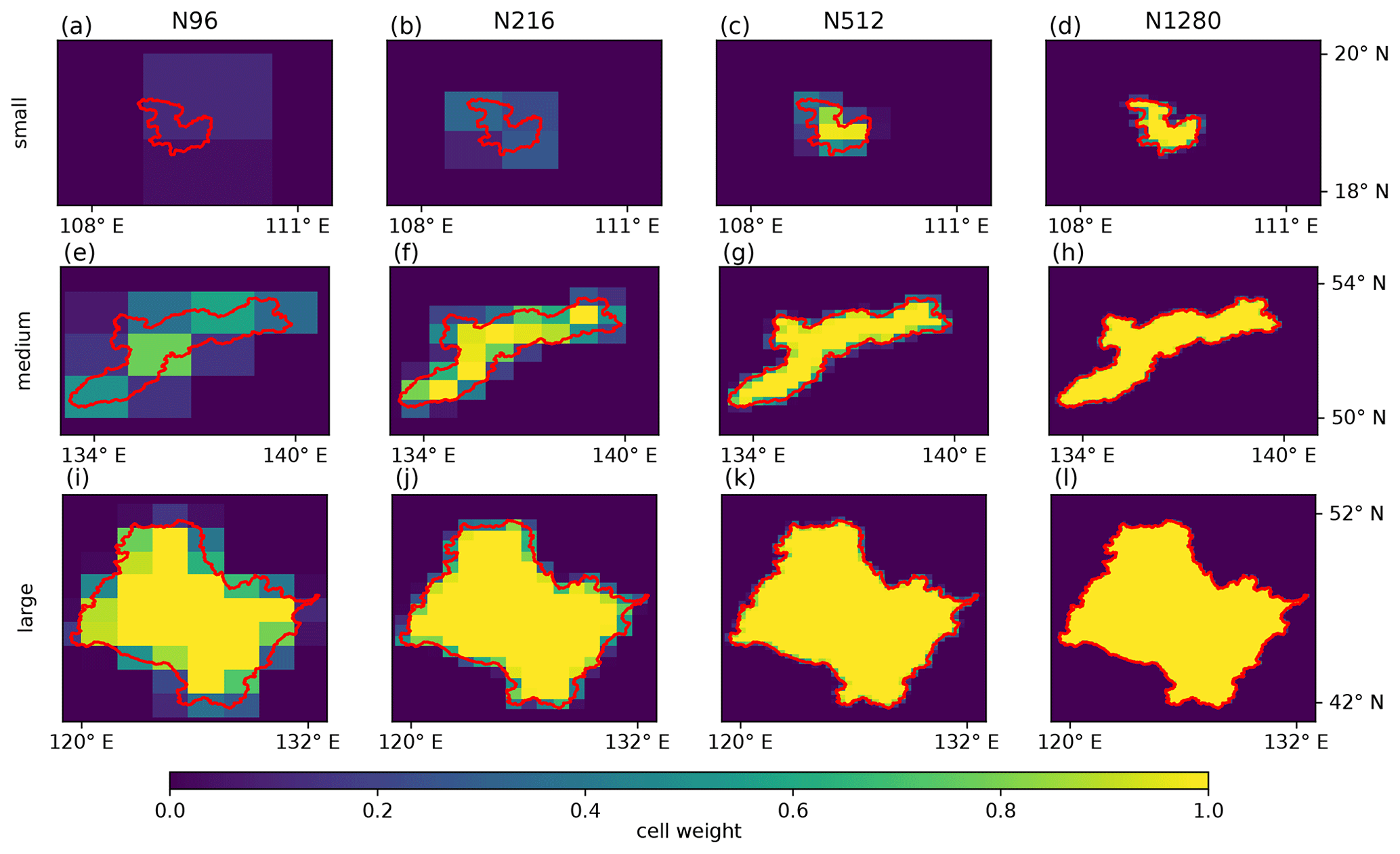
Figure 1Weights used in the gridded representation of example basins at different resolutions. The basin with the median area from each of the basin scales in Table 2 is shown in each row, and each column shows the different simulation resolutions used in this study. The small, medium and large basins shown have areas of 5040, 54 600 and 553 000 km2 respectively.
It is clear that, at lower resolutions, the smallest basins cover substantially less than one grid cell (e.g. Fig. 1a). We choose to perform the analyses at these scales for the coarse resolutions because, even though each basin is poorly represented by any one grid cell, the statistical picture that is created by aggregating over many such basins should still be accurate. This choice is somewhat validated by the evaluations between CMORPH and the simulations shown in Figs. 5 and 8, which show that the different-resolution simulations exhibit plausible relationships, even at the finest basin scale.
2.4.3 Spatial averages over basins
We complete the analysis by computing spatial means over each of the basins. For JJA mean precipitation, we use an area-weighted mean over each basin, also using the basin weights:
Here, Pj is the precipitation in the jth cell, and is the mean precipitation in the ith basin. The summation is over all N grid cells, and the area weights are the same for all cells at a given latitude. The area weights for each grid cell, Warea,j, are calculated to ensure that grid cells further north, which will be smaller on a latitude–longitude grid, contribute less to the mean. The basin weights for each basin i and each grid cell j, , are as described above (Sect. 2.4.2).
Producing the basin-weighted diurnal cycle requires the production of a composite diurnal cycle over the weighted grid cells that comprise each basin. We do this by taking the spatial mean of the diurnal cycle in each grid cell, weighted by the basin weights and an area weighting as above. For example, for the basin-mean diurnal cycle of amount, , at each time t over the day,
where Aj(t) is the amount at time t in grid cell j. The diurnal cycles of frequency and intensity have the same equation, replacing A with F or I. From the diurnal cycle of A over a basin, the phase of the peak and the amplitude of the diurnal cycle are calculated using harmonic analysis as above (Sect. 2.3).
2.4.4 Basin-scale error statistics
To compare the simulations with the CMORPH observations, we use basin-level error metrics. For example, we use the RMSE to compare the mean JJA precipitation between CMORPH and each of the simulations, as defined by
Here, there are Nbasin basins, and so the summation is over all basins. is the mean precipitation in basin i in the observations, and is the mean precipitation in basin i for the simulation.
When comparing the phase ϕ of the peak of A, F or I between simulations and observations, it is necessary to take into account the fact that this is a circular quantity. That is, a phase at 23:00 LST should be 2 h away from 01:00 LST, not 22 h away. This is achieved by applying a base-24 circular difference (circular diff24(x)) operation to the difference between observations and simulations to calculate a circular RMSE:
In Fig. 2, the regions of interest in this study are shown. The full domain encompasses the top-level HydroBASINS Asia region. Results from this region are discussed in Sect. 3. Because the orography is important for determining where and when precipitation occurs, the terrain over the top-level HydroBASINS Asia region is shown. The most prominent feature is the Tibetan Plateau; we are interested in the effect that it has on precipitation, particularly that of its southern flank. The Sichuan Basin can also be distinguished, where the diurnal cycle of precipitation exhibits a clear phase propagation (Li et al., 2020). In Sect. 4, we will focus on the south-east of China, shown by the black rectangle, in Figs. 9 and 10 below, so as to directly compare with previous results from a regional UM configuration (Li et al., 2018).
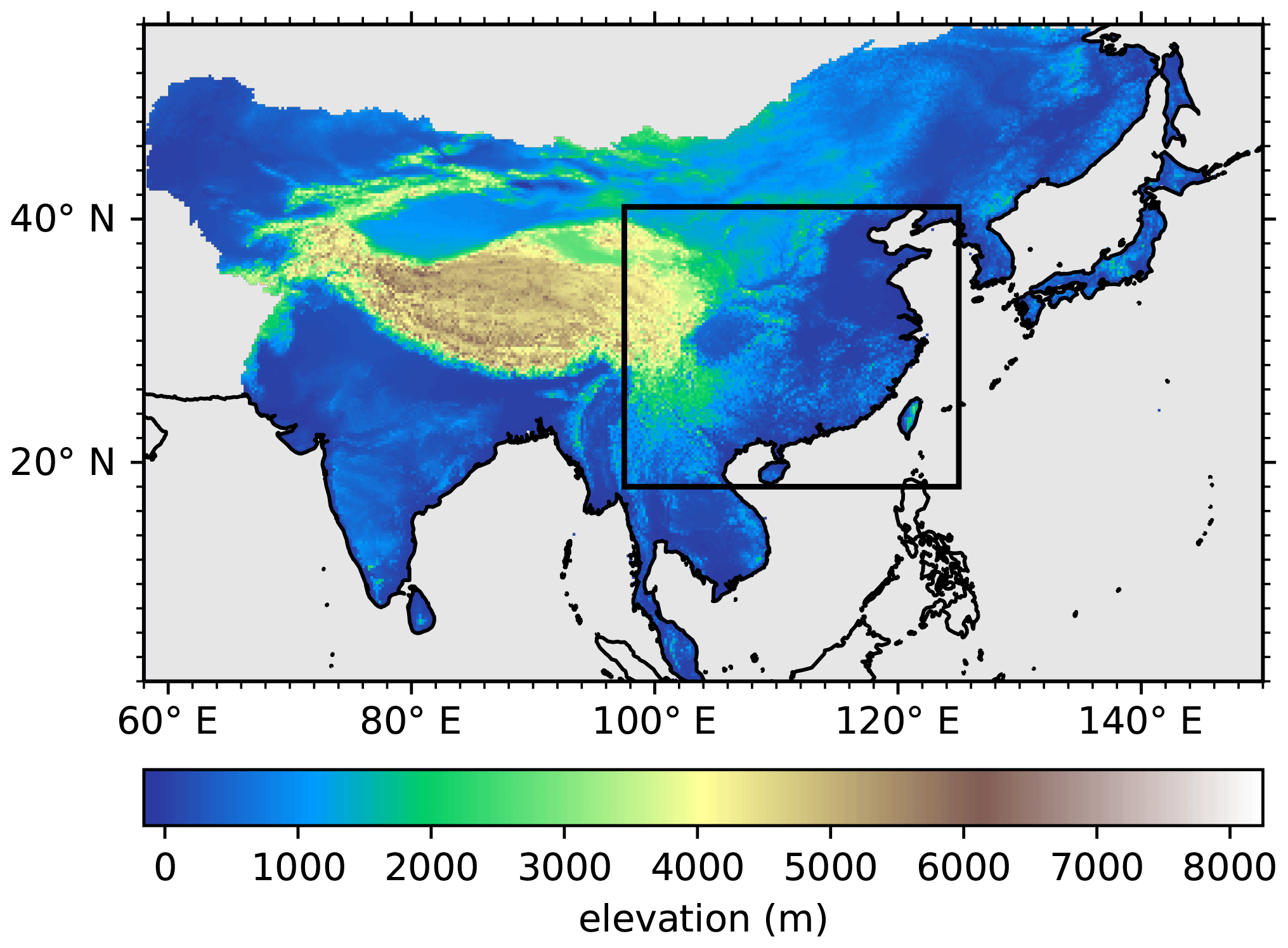
Figure 2Asia, as represented by the HydroBASINS level-1 dataset (coloured), showing the terrain elevation. The black rectangle is the region of interest over south-eastern China shown in Figs. 9 and 10. Prominent features which are discussed are the Tibetan Plateau, particularly the Himalayas on its southern flank. Also, the diurnal cycle over the Sichuan Basin (centred on 30∘ N, 106∘ E) will be discussed. The 30 arcsec elevation data from the HydroSHEDS dataset (Sect. 2.4.1) are shown.
3.1 Mean precipitation
In Fig. 3, the mean JJA precipitation over Asia from observations and simulations is shown. In the following, we mainly discuss the features over land. From the observations, several prominent features are visible. There is a strong band of precipitation off the western coast of India, which is related to the ISM flow. Precipitation falls at a rate of 2–4 mm d−1 over southern India east of the Western Ghats mountains, with substantially higher rates over northern India. Both of these are consistent with other studies of the ISM (e.g. Mitra et al., 2013). Along the Himalayas, there are very high local maxima of precipitation of 12 mm d−1. This is due to the ISM flow interacting with the high orography and associated steep gradients of the Tibetan Plateau and the Himalayas (Fig. 2). Some scattered points with high precipitation rates over the body of the Tibetan Plateau are an artefact of the satellite retrieval method and due to the snow cover in this region (Joyce et al., 2004).
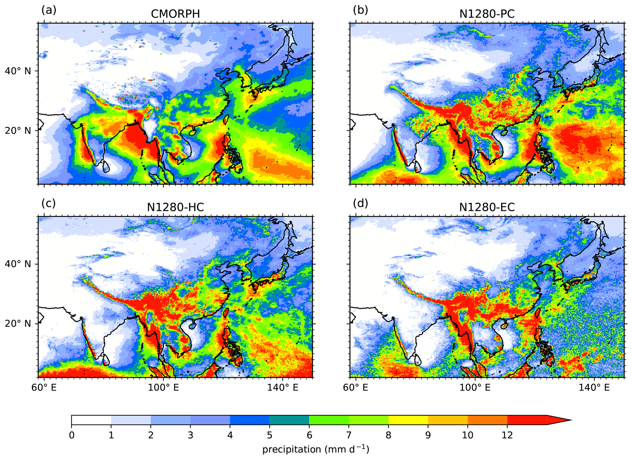
Figure 3Mean JJA daily precipitation over Asia for CMORPH observations (a) and the parametrized (b), hybrid (c) and explicit (d) convection simulations. The observations are taken from 1988 to 2018, and the simulations are all from 2005 to 2008. Note that in this figure we show mean precipitation, and in subsequent figures we show amount of precipitation; these two quantities are close to each other but not identical as amount of precipitation has very low values, under 0.1 mm h−1, thresholded out (Sect. 2.3).
Over south-eastern China, high precipitation rates of 6–12 mm d−1 are seen. This is associated with the EASM and the propagation of the Meiyu front, both of which are active during JJA. Further inland, there is a small secondary maximum at around 28∘ N, 102∘ E, which is related to the orography of the Tibetan Plateau on the north-western boundary of the Sichuan Basin.
A large area of intermediate summer rainfall (2–5 mm d−1) is seen over north-eastern China at higher latitudes. A maximum in seasonal JJA precipitation is seen over and near the Korean Peninsula. Over the Gobi and Taklamakan deserts, less than 1 mm d−1 occurs in JJA.
Over the ocean, the western tongue of the intertropical convergence zone (ITCZ) is clearly visible. Precipitation rates are high to the west of the Philippines, off the southern coast of Japan, and over a large area of the Bay of Bengal.
The simulations broadly reproduce the observed Asian summer precipitation distribution. The low precipitation rate over the deserts is well matched. The magnitude and extent of precipitation in north-eastern China are accurately reproduced, although N1280-EC produces some localized areas of higher precipitation and N1280-PC fails to produce the maxima over the Korean Peninsula. However, at lower latitudes there are substantial differences. Over China, the simulations produce too much precipitation, with maximum rain rates of over 12 mm d−1 over much larger areas than in the observations. Precipitation rates over India are much lower in the simulations than the observations – a known bias of the UM (Bush et al., 2015). N1280-EC in particular has very low rain rates over India (particularly north-eastern India), with no signal of the higher rates seen at 20∘ N in observations. An intriguing possibility is that this is due to a lack of Bay of Bengal depressions forming in N1280-EC, although we have not investigated this here. Clearly the lack of a convection parametrization affects the simulation to a large degree over this region. There are signs of a large, spurious maximum of precipitation over the Indian Ocean in all the simulations, which has been linked to the dry bias over India in the UM (Bush et al., 2015) and also in multiple other GCMs (e.g. Bollasina and Ming, 2013; Levine et al., 2013). Over land, N1280-EC and N1280-HC closely resemble each other.
All the simulations produce high rates of precipitation over the Himalayas, although N1280-PC produces a band of precipitation which is too wide. Both N1280-EC and N1280-HC produce maximum precipitation rates which are too high, particularly close to 100∘ E. This is consistent with Willetts et al. (2017), who found that shorter-duration explicit simulations with 12 km grid lengths produced excessive precipitation over the Himalayas. Furthermore, this bias is increased at higher resolutions compared to lower resolutions (not shown), which indicates that the high-resolution simulations are producing too much orographic precipitation.
Over the western Pacific, the N1280-PC simulation produces far too heavy precipitation over far too large an area, whereas the opposite is true for N1280-EC. N1280-HC has smaller precipitation biases against observations. All the simulations produce heavier precipitation west of the Philippines, consistent with observations. All the simulations produce less precipitation than observed over the Bay of Bengal.
3.2 Mean precipitation over catchment basins
In Fig. 4, the precipitation rates in Fig. 3 are averaged over basins of different scales. Thus, Fig. 4a, which shows the CMORPH observations averaged over the small basin scale (see Table 2), resembles Fig. 3a. As noted in Sect. 2.4.2, the basin-selection algorithm cannot pick basins in a given scale range that completely cover the Asian land, and hence there are gaps at each basin scale. As is clear from Fig. 4a to c, averaging over larger basin scales reduces the maximum precipitation rates at that scale, since high precipitation rates are averaged with lower rates.
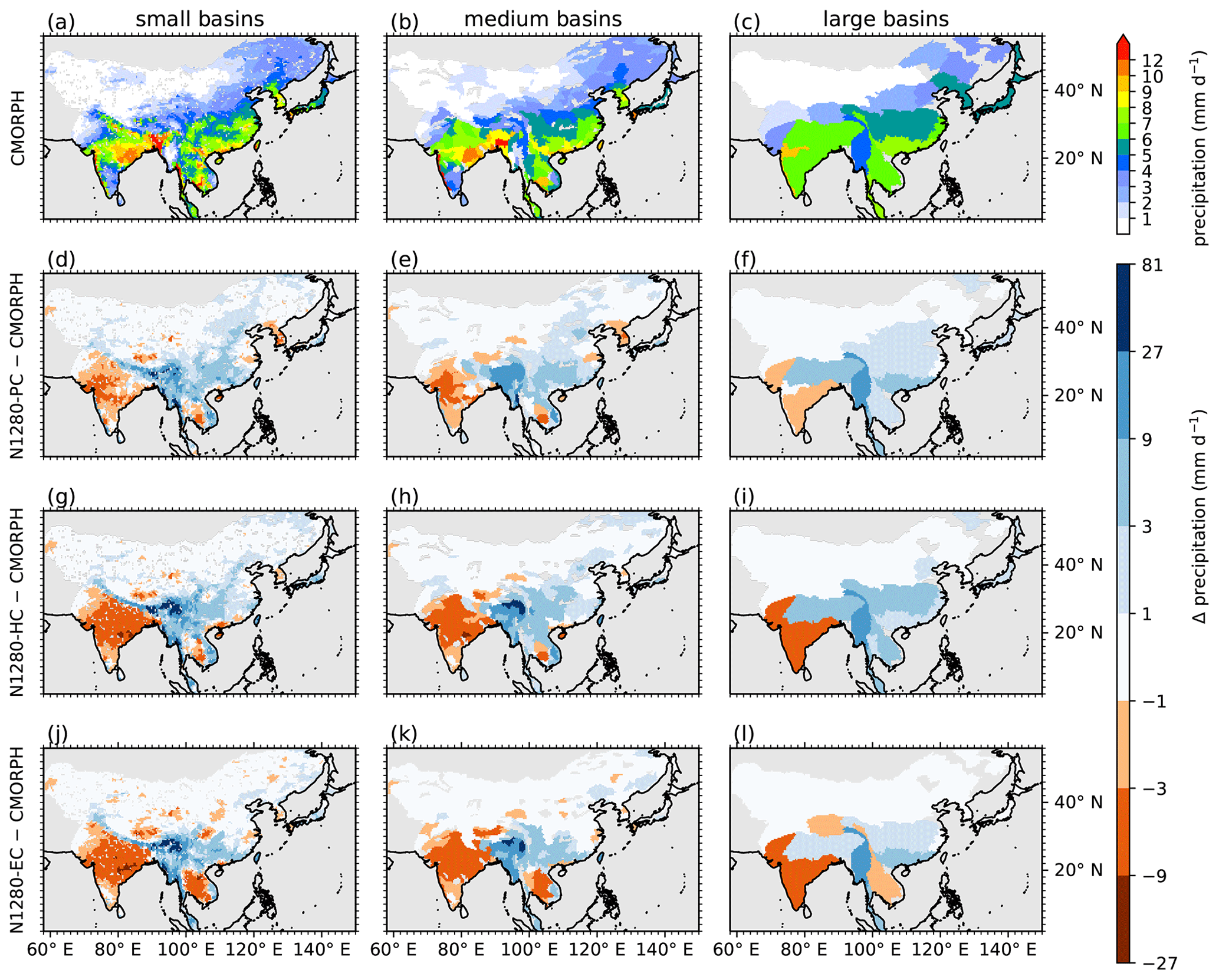
Figure 4Mean JJA precipitation over Asia averaged over basins of different scales showing CMORPH (a–c) and difference between simulations and CMORPH for N1280-PC (d–f), N1280-HC (g–i) and N1280-EC (j–l). One basin scale is shown in each column, and one dataset is shown in each row. Areas shown in grey are not covered by selected basins (see Sect. 2.4.1 and 2.4.2).
The small basin-scale column provides some more details of what was seen in Fig. 3. Both simulations produce too little precipitation over India; this is particularly the case for N1280-EC at around 20∘ N. Both simulations produce too much precipitation on the Himalayas, with N1280-EC producing up to 72 mm d−1 more precipitation at 95∘ E than CMORPH. The basins with the maximum precipitation rates in N1280-PC and N1280-EC have rates that are respectively 7 and 11 times higher than CMORPH. These biases dominate the differences between the simulations and observations; the increased precipitation over south-eastern China in the simulations is present but is smaller in magnitude. Similarly, the differences in precipitation rates between the simulations and CMORPH in north-eastern China are barely visible, as the magnitude of the precipitation in this region is typically low to begin with in both observations and simulations (Figs. 3 and 4a, d, g and j). There are few differences between N1280-EC and N1280-HC. Both simulations produce a dry bias over the Indochina Peninsula, although the spatial extent of this is larger for N1280-EC. Likewise, the dry bias over the Sichuan Basin in N1280-EC is larger than that in N1280-HC.
At the small basin scale, the HadGEM3-GC3.1 simulations at coarser resolutions (N512-PC, N216-PC and N96-PC) produce mean JJA precipitation over Asia that most closely resembles N1280-PC (not shown). The highest resolution of these simulations, N512-PC, is most similar to N1280-PC, although it has slightly enhanced precipitation (1 mm d−1) over India and slightly reduced precipitation (1–4 mm d−1) over China. N216-PC is less similar to N1280-PC than N512-PC. N216-PC produces less precipitation than N512-PC and N1280-PC over the Western Ghats on the western coast of India, presumably due to under-resolved orography, and produces more precipitation than N512-PC and N1280-PC over north-eastern China. N96-PC is least similar to N1280-PC. Again, there is less precipitation compared to N1280-PC over the Western Ghats, presumably because of under-resolved orography. A lack of precipitation over India is evident, as in the simulations of Bush et al. (2015). These broad comparisons are true at all basin scales.
For medium and large basin scales, there are smaller discrepancies between the simulations and observations as precipitation is averaged over larger basin scales. This is partly because averaging over a larger area smooths out the signal of localized maxima in precipitation, as mentioned above. We also expect to extract useful information about how the model represents precipitation at different spatial scales by calculating statistics about the agreement between the simulations and observations. In Fig. 5, basin-scale RMSE values (Sect. 2.4.4), calculated between the JJA mean precipitation in CMORPH and the simulations, are shown as a function of scale. As noted in Sect. 2.4.2, we perform the analysis at 11 different basin scales, ranging from small to large, spaced equally on a logarithmic scale. We also include the three lower-resolution simulations: N512-PC, N216-PC and N96-PC (Table 1). For all the simulations, averaging over a larger basin scale improves the error statistics by reducing the RMSE as the basin scale increases.
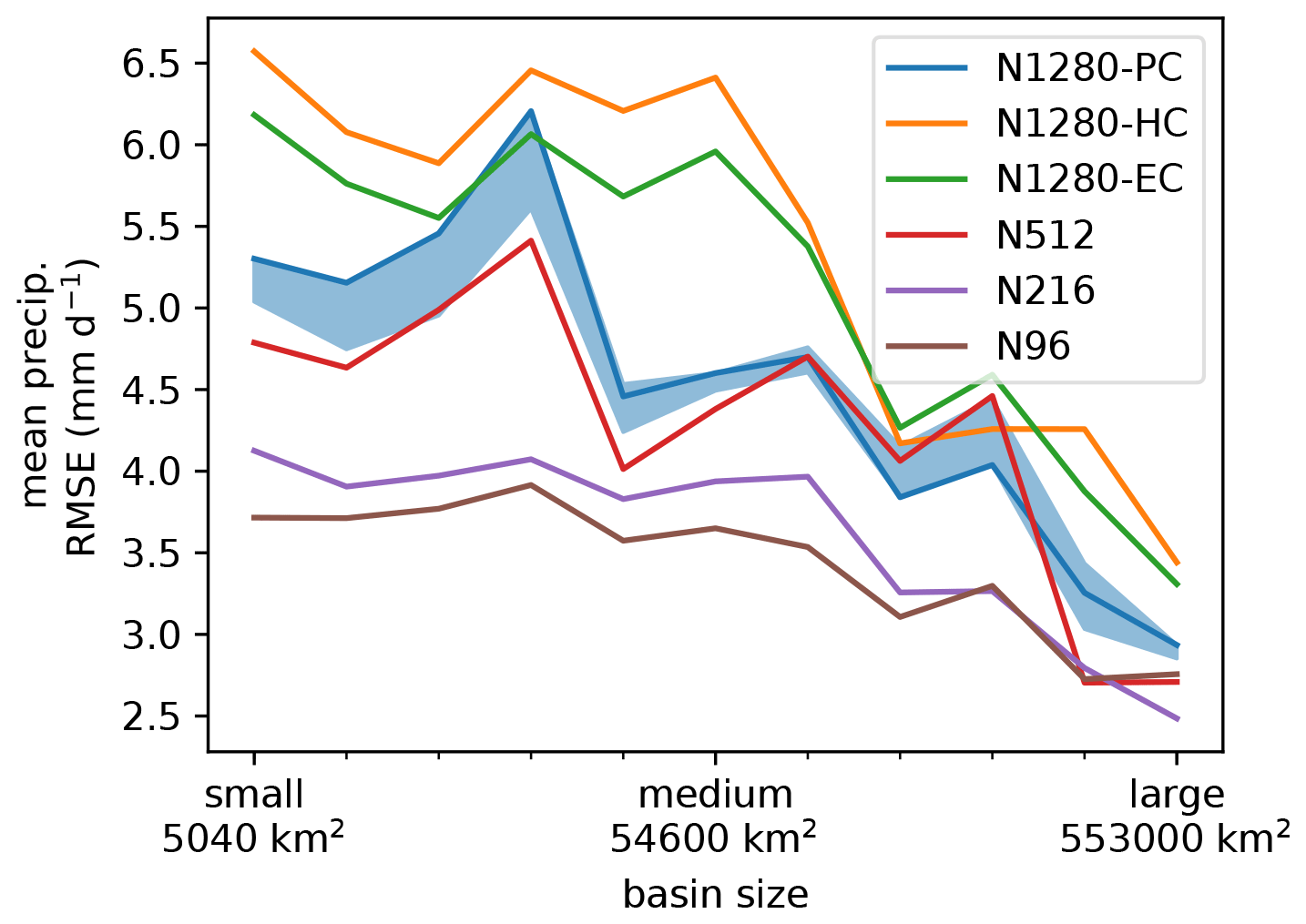
Figure 5Basin RMSE (Sect. 2.4.4) of each simulation compared to CMORPH shown as a function of basin scale. Light blue shading shows the maximum spread for the three N1280-PC ensemble members. The basin name and median basin size are shown on the x axis.

Figure 6The diurnal cycle of the amount, frequency and intensity of precipitation over Asia for CMORPH and the three high-resolution simulations, showing the phase in LST in colour and the amplitude by the opacity of the colour. The diurnal cycle is considered strong if its amplitude is in the top third of the Asia-wide amplitudes over the whole domain (including oceans), weak if it is in the bottom third and medium otherwise (Sect. 2.3). Note that the strength of the diurnal cycle is calculated separately for each dataset. Thus, it is possible to say that all datasets have a weak diurnal cycle for the amount of precipitation over the north-western region of the domain but not that the magnitude of the amount is similar where the diurnal cycle is considered strong. An absolute comparison is done in Fig. 8.
We note that the N96-PC simulation performs best by these metrics. This is because N96-PC produces much lower precipitation maxima and therefore is penalized less than the other five simulations for producing too much precipitation over e.g. the Himalayas. Indeed, the error increases with resolution for all spatial scales. The spread between the three N1280-PC ensemble members is typically smaller than the difference between that simulation and the other simulations. When the three high-resolution simulations are compared, N1280-EC and N1280-HC perform worse than N1280-PC, with N1280-HC performing slightly worse than N1280-EC. Again, this is due to excessive precipitation in the simulations with explicit deep convection. This shows that disabling the convection parametrization has an important bearing on performance for climatological JJA precipitation.
We have performed identical analysis comparing the simulations to APHRODITE (Sect. 2.1.2). The equivalent figure to Fig. 5 (Fig. S3) is very similar, and qualitatively the same conclusions would be drawn. This shows that the difference for this metric between the simulations and observations is larger than the differences between the observational products.
3.3 Diurnal cycle
Figure 6 shows the diurnal cycle over Asia in the CMORPH observations. As also seen below in Sect. 4.2 for south-eastern China, the amount and intensity of precipitation are highly similar. For both of these, there is a marked difference between land and ocean, both in the phase and amplitude of the diurnal cycle: over land the amplitude is larger and the phase is later. The phase over the ocean tends to be either early morning (03:00–07:00 LST) over the ITCZ and off the coast of Japan or close to midday off the coast of China. There is an interesting phase delay off the eastern coast of India over the Bay of Bengal, as the phase of the diurnal cycle goes from 08:00 to 17:00 LST. This feature has been noted in previous studies (e.g. Yang and Slingo, 2001): it is thought to be related to the coupling between gravity waves and convection, leading to long-lived mesoscale convective systems (Houze, 2004).
Over land, the diurnal cycles of the amount and frequency of precipitation show some clear features. North of 35∘N, the amplitude of the diurnal cycle is typically weak and the peak has a phase of 15:00–18:00 LST. Closer to the Equator, the amplitude of the diurnal cycle is generally strong, consistent with the stronger diurnal solar forcing in the tropics. India can be divided into two main regions. Central India shows a peak of precipitation in the late evening. Coastal western India, north-eastern India and north of about 20∘ N show an early evening peak. The southern flank of the Tibetan Plateau shows an interesting phase delay from north to south, with a late-night peak in precipitation close to the Plateau top progressing to an early morning peak (08:00 LST) further south.
The diurnal cycle field for intensity of precipitation is noisier. In general, late-night peaks in amount, frequency and intensity are co-located. We speculate that this could be due to the activity of mesoscale convective systems, which are associated with both convective and stratiform precipitation. The convective precipitation would likely affect the intensity of precipitation, whereas the combined convective and stratiform precipitation would affect the amount, frequency and intensity of precipitation. For intensity, some areas show broadly similar signals to those for amount and frequency, such as the phase delay over the Bay of Bengal, the pattern over the ocean and the phase delay on the southern flank of the Tibetan Plateau. However, some regions show substantial differences. At higher latitudes over land, the peak of intensity is 4–6 h later than the peaks of amount and frequency. This potentially indicates that convective precipitation is dominant later during the day in these regions.
We can compare the simulations to the observations (Fig. 6), noting again that the observations span 21 years and that the simulations span 4 years. This leads to the simulations being noisier than the observations. Before presenting a detailed analysis, we note that N1280-EC produces a more realistic diurnal cycle in most regards than either N1280-PC or N1280-HC. In N1280-EC, over land the phase of the diurnal cycle better matches the observations for both amount and frequency and is marginally better for intensity. The land–sea contrast is better represented, for example off the coast of south-eastern China. The similarity of the diurnal cycles of amount and frequency in N1280-EC is closer to that of the observations. Thus, in terms of producing a realistic diurnal cycle, the lack of parametrized convection is clearly an advantage.
Perhaps the most striking differences between the simulations and observations are for N1280-PC frequency and amount. For frequency, this simulation shows a peak over almost all of Asia that is far too uniform and too early, being close to local midday. It is well known that convection parametrization schemes respond to the peak in insolation forcing by producing convective precipitation (e.g. Yang and Slingo, 2001; Stirling and Stratton, 2012; Bechtold et al., 2014), which is certainly one of the reasons for this signal. Evidence for this is also seen in Bougeault and Geleyn (1989), who found that no precipitation was detected before local midday in a simulation with explicit convection, whereas in parametrized simulations too much rainfall is produced before midday. For intensity, the peak over almost all of Asia is close to local midnight. For N1280-PC, the peak in precipitation amount is also clearly biased to be too early, although it does show greater spatial variation than the frequency or intensity over this region. Additionally, there are differences between amount and frequency, even though this is not seen in the observations. There are few differences between the different N1280-PC ensemble members (not shown). The largest difference is for the phase of precipitation amount over eastern India, although in general the phase and amplitude are very similar among ensemble members.
For N1280-EC over land, the phases of the peaks for amount and frequency broadly agree, although this simulation appears to produce too little late-night precipitation. Additionally, the phases for all three precipitation measures over the ocean match the observed phases quite closely, although they are noisier for the simulation. Likewise, the amount and frequency are fairly similar for this simulation, although the similarity is not as strong as it is for the observations. N1280-EC does capture some aspects of the phase of the intensity field in the observations, such as the late-night peaks over India and the Indochina Peninsula. However, there are pronounced differences between N1280-EC and the observations. From the peak in amount of precipitation over India, the amplitude of the diurnal cycle is too weak. This is probably due to the dry bias in this region (Fig. 3c). N1280-EC produces a peak in intensity of precipitation that is too noisy, which is probably related to the shorter duration of the simulation. The peak in intensity is also weak, particularly over the Tibetan Plateau. However, this is a region with known biases in CMORPH (Joyce et al., 2004), so any comparisons to CMORPH in this region should be made with caution.
N1280-HC shares some similarities to both N1280-PC and N1280-EC, which makes sense given its hybrid representation of convection. Its diurnal cycle of the amount of precipitation resembles N1280-EC. This could indicate that the convective precipitation that is caused by deep convection is primarily responsible for the diurnal cycle of the amount of precipitation, as both simulations represent deep convection explicitly. For the diurnal cycle of the frequency of precipitation, N1280-HC more closely resembles N1280-PC, although it shows more spatial variation over land. The resemblance potentially indicates that the shallow and mid-level parametrizations of convection are responsible for this diurnal cycle. The fact that the N1280-HC amount and frequency diurnal cycles do not closely resemble each other means N1280-HC is less like the observations (Fig. 6). The diurnal cycle for the intensity is stronger over land in N1280-HC than N1280-EC, meaning N1280-HC matches the observations more closely and indicating that there may be issues with the representation of this diurnal cycle in N1280-EC.
Over the ocean, the N1280-PC simulation does not match the observations particularly closely, whereas the N1280-EC simulation performs better, with N1280-HC falling in between. All the simulations show hints of a phase delay of the peak in amount and frequency of precipitation over the Bay of Bengal, indicating that the simulations might capture the important aspects of the coupling between convection and gravity waves. However, all show significant biases: N1280-PC is too early close to the coast of India, and N1280-EC and N1280-HC are too weak and too late. N1280-PC produces diurnal cycles which have substantial biases in phase and amplitude over all other areas of the ocean for all three of amount, frequency and intensity. N1280-EC in general produces more realistic phases and produces slightly more realistic peaks in amount and frequency over the western Pacific and between the Philippines and the Indochina Peninsula. However, it is noisier than the observations, which is probably due to its shorter duration. The phase of the intensity of precipitation in N1280-EC does not match observations particularly closely, being stronger and too uniform and in general occurring later in N1280-EC than the observations. N1280-HC is again closer to N1280-EC in amount and N1280-PC in frequency and intensity. It has a particularly strong diurnal cycle near midnight for frequency over the western Pacific that is not evident in the observations, which is perhaps related to its wet bias at that location (Fig. 3).
3.4 Diurnal cycle over catchment basins
As with the mean precipitation (Sect. 3.1), the phase and amplitude of the diurnal cycle can be averaged over catchment basins of different spatial scales (see Sect. 2.4.2 for details). Figure 7 shows this over Asia for CMORPH, N1280-PC, N1280-HC and N1280-EC over small, medium and large basin scales for the amount of precipitation. Figure 7a, the CMORPH observations, is similar to Fig. 6a, as the basins are small, and likewise for the simulations (Fig. 7d, g and j).
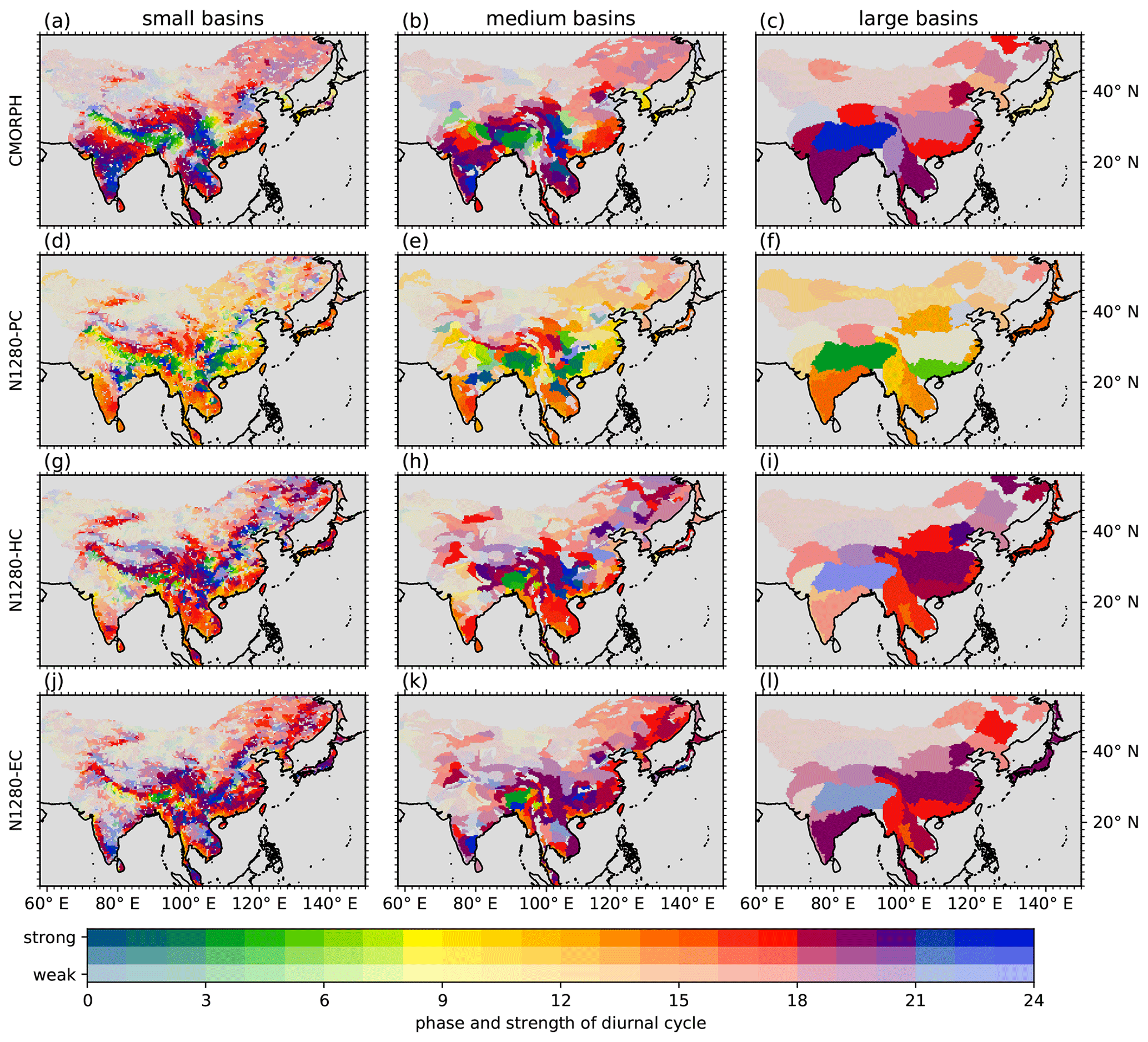
Figure 7Diurnal cycle of amount of precipitation over Asia averaged over different basin scales (columns) for CMORPH, N1280-PC, N1280-HC and N1280-EC (rows). As described in Sect. 2.3 and as in Fig. 10, a visual representation of the amplitude is given by its strength, dependent on whether it is strong, medium or weak. This is calculated separately for each dataset and scale (i.e. for each panel).
For the observations, averaging the diurnal cycle over larger basin scales yields useful information about the phase and amplitude of the diurnal cycle at different scales. This information is similar in spirit to that presented in Covey et al. (2016), although the method they used relied on vector averaging, whereas the method in this study uses direct averaging of the diurnal cycle at each grid point (Sect. 2.4.2). They recommend using their method to compare CMIP5 simulations with observations to give a sense of how well the diurnal cycle is represented. However, whereas they average over all land and ocean grid points, we use a much finer-grained approach of averaging over catchment basins over land. This allows us to distinguish between the phase and amplitude of the diurnal cycle over specific regions and allows us to compare simulations and observations as a function of spatial scale.
For the observations, as the diurnal cycle is averaged over larger scales, certain information comes to the fore, and at the same time location-specific detail is lost. For example, over northern India and Nepal, from Fig. 7a there is fine-scale detail in terms of the phase delay on the southern flank of the Tibetan Plateau, whereas this is no longer detectable over medium-sized basins – where it averages to around 06:00 LST. Furthermore, comparing Fig. 7b and c, the detail of the late-night phase over southern India is clearly lost at the large scales. However, at the large scale, a continent-wide pattern emerges that is hard to discern at the finer scales – that over southern India on average the diurnal cycle is strong and occurs at 19:00 LST. Thus, the large basin scale yields information about the overall behaviour of the diurnal cycle, which can be compared against its behaviour in simulations – similarly to Covey et al. (2016). Additionally, averaging over larger spatial scales will reduce the noise in the shorter-duration simulations and so should produce a fairer comparison between the simulations and the observations.
At small basin scales N1280-PC performs poorly for the diurnal cycle in the amount of precipitation (it performs worse for frequency and intensity of precipitation, not shown). It does not improve when the analysis is performed at the large basin scale. From the large scale, N1280-PC produces a diurnal cycle that peaks too early in the day, e.g. over India, where it occurs at 14:00 LST in the simulation and at 19:00 LST in the observations. In comparison, at the large scale, N1280-EC broadly agrees with the observations, producing phases over different regions such as southern India and the southern coast of China, which are much closer to the observations. There are regions that do not match so well, such as northern India, where the diurnal cycle in the simulation is far too weak, although the phase matches more closely. This weak diurnal cycle can be attributed to the dry bias in this simulation (Sect. 2.4.2). N1280-HC produces a diurnal cycle of amount of precipitation that is quite similar to that of N1280-EC. Some differences are evident at the smallest basin scales. The phase of the diurnal cycle is earlier over coastal south-eastern China, which means that N1280-HC matches CMORPH more closely. However, the phase is also earlier over the Indochina Peninsula, which means that it matches CMORPH less closely.
The N96-PC, N216-PC and N512-PC simulations all strongly resemble N1280-PC (not shown), suggesting that the convection parametrization scheme, and not model resolution, is responsible for producing the diurnal cycle in the simulations.
In Fig. 8, we compare the simulations to observations at different spatial scales. Error statistics appropriate for the phase and amplitude are shown for amount, frequency and intensity for all the simulations against CMORPH as a function of basin scale (the error statistics are described in Sect. 2.4.4).

Figure 8Basin error statistics (Sect. 2.4.4) of the diurnal cycle phase and amplitude of each simulation compared to CMORPH shown as a function of basin scale. Amount, frequency and intensity are shown in each column, and the error statistics appropriate for phase, amplitude and both combined are shown in each row. Light blue shading shows the maximum spread for the three N1280-PC ensemble members. The basin names and median basin sizes are shown on the x axis.
For the phase, the clear signal is that for amount, frequency and intensity N1280-EC performs best, with N1280-HC performing almost as well. Indeed, for amount of precipitation, all the simulations with parametrized convection perform worse as spatial scale increases to the large basin scale; only N1280-EC and N1280-HC improve as spatial scale increases. For frequency and intensity, all the simulations improve as spatial scale increases, although again N1280-EC shows the most improvement (particularly for frequency). It is remarkable that the parametrized convection simulations span a range of resolutions from 14 to 180 km, yet their error statistics are very similar across all three measures of precipitation (particularly so for frequency). Where there is some resolution sensitivity, the performance improves as resolution increases – e.g. amount at all spatial scales.
The main difference between N1280-EC and N1280-HC is that the latter performs better for the amplitude of the intensity. For the amount of precipitation, all the simulations perform better at larger spatial scales. N1280-EC performs worst at the finer scales. The same is broadly true for intensity, although the improvement at larger scales is less pronounced. For frequency, all the parametrized simulations perform poorly.
In this section, we focus on south-eastern China (Fig. 2, black rectangle) for straightforward comparison with Li et al. (2018). In Sect. 4.1, we analyse the amount, frequency and intensity of precipitation, and in Sect. 4.2 we analyse their diurnal cycles.
4.1 Amount, frequency and intensity of precipitation
The amount, frequency and intensity of precipitation are shown in Fig. 9 for JJA in south-eastern China. The threshold for the analysis is 0.1 mm h−1. The amount, averaged over 1 d, is very similar to the mean precipitation, although the thresholding means that the values are not identical. Thus, CMORPH amount, Fig. 9a, is effectively the same as Fig. 3a but for China instead of Asia, and likewise for the N1280-PC and N1280-EC amount. The results shown here are directly comparable to those in Li et al. (2018), who analyse precipitation in two regional UM simulations against gauge-based observations. Their simulations are run at 4.4 and 13 km grid lengths, with explicit and parametrized convection respectively, for the warm season of 2009, encompassing JJA. Both their simulations use boundary conditions provided by a global UM run with a grid length of 0.2∘. All their simulations use the GA6.1 science settings (Walters et al., 2017). To facilitate the comparison, we only show and discuss results from N1280-PC and N1280-EC here, omitting N1280-HC (Figs. S4 and S5 show N1280-HC and are equivalent to Figs. 9 and 10).
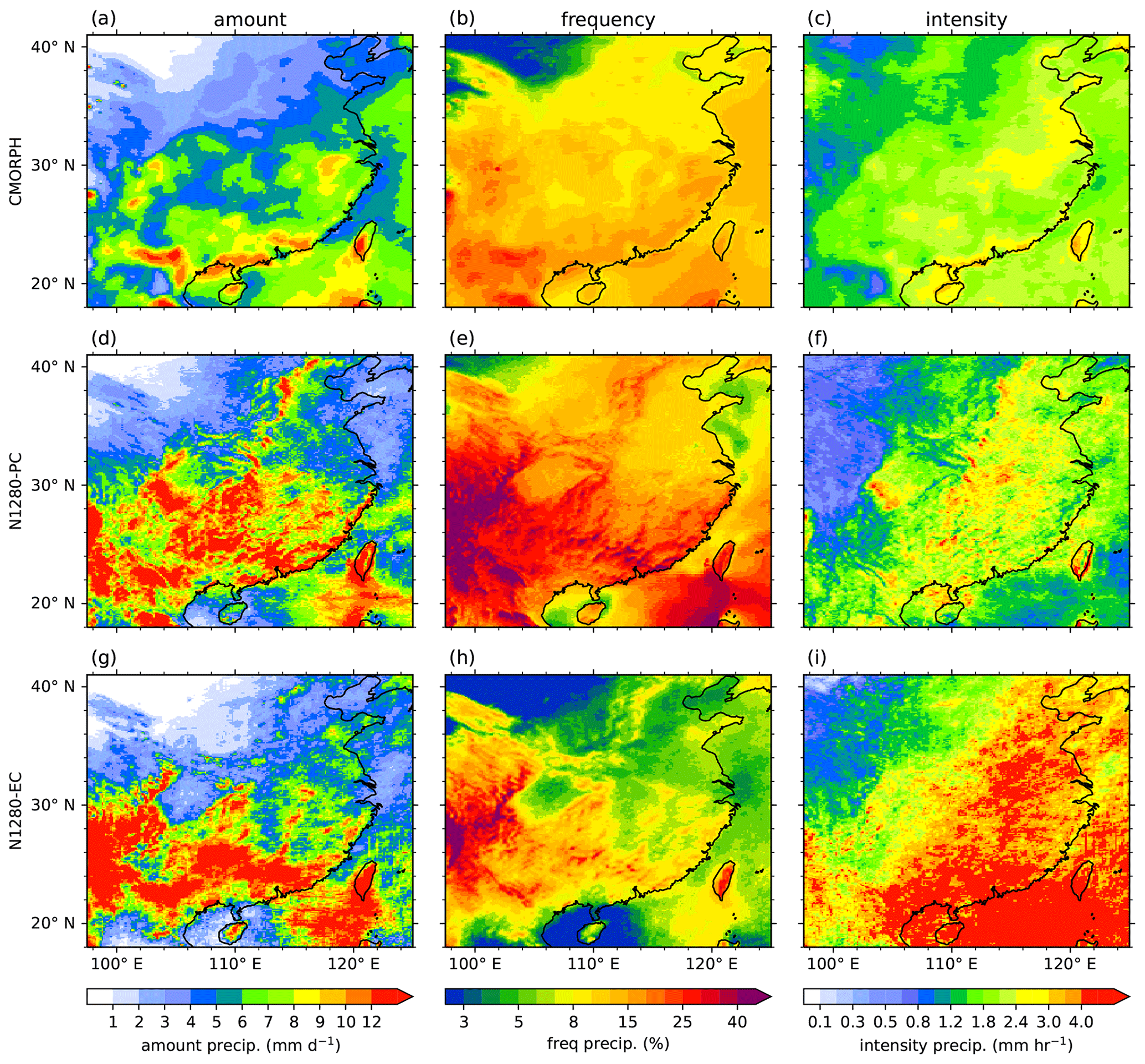
Figure 9Amount, frequency and intensity of precipitation (columns) over China for CMORPH (a–c), N1280-PC (d–f) and N1280-EC (g–i).
For the CMORPH amount, there are localized maxima near south-facing coasts, indicating that the moist EASM flow in JJA produces precipitation when it passes over land. These are linked to higher-intensity precipitation near the coast (Fig. 9c). There is a maximum near 23∘ N, 104∘ E, which appears to be related to particularly frequent precipitation. For amount, there is generally a decreasing gradient in precipitation going further inland, with local inland maxima and minima typically related to the orography.
Amount, frequency and intensity in CMORPH over south-eastern China are similar to Zhou et al. (2008), Figs. 2c, f and i, which show the Tropical Rainfall Measuring Mission (TRMM) satellite product. This is despite the fact that they use a different satellite product, a threshold of 0.2 mm h−1 (which will affect frequency and intensity), and a shorter time period of 2000–2004. The similarity indicates three things: that amount, frequency and intensity in CMORPH are broadly similar to those in TRMM, that a shorter time period is able to represent the mean of these precipitation measures, and that the quantitative values are affected by the threshold, but the qualitative conclusions are broadly the same for different thresholds.
From N1280-PC and N1280-EC amount, both simulations produce too much precipitation over the majority of south-eastern China. In the Sichuan Basin, both simulations produce amounts of precipitation that are too low, and this is pronounced in N1280-EC. This is due to less frequent precipitation in this region (Fig. 9e and h). The overestimation of precipitation in N1280-PC is due to too frequent precipitation, as can be seen by comparing Fig. 9b and e. However, in N1280-EC the frequency matches CMORPH more closely east of 104∘ E (notwithstanding the bias in the Sichuan Basin), and the bias in precipitation rates is due more to the intensity bias (Fig. 9c and i). West of 104∘ E, the wet bias in N1280-EC appears to be related to both frequency and intensity being too high. N1280-EC produces very intense precipitation over the sea, and there is a marked land–sea contrast that is not present in either CMORPH or N1280-PC.
Comparing with Fig. 2 from Li et al. (2018) is instructive. Comparing the observations (CMORPH here and gauge stations in their study) reveals that they both produce similar patterns of amount of precipitation. In Li et al. (2018) they only sample from 1 year, whereas this study uses a 21-year duration, and hence their Fig. 2a is noisier. We note that the frequency and intensity fields in both studies are qualitatively similar. However, in Fig. 9b the frequency is generally higher than that in Li et al. (2018), and correspondingly the intensity is less in this study. This could be due to the method they used to turn the point gauge observations into a continuous field, as both studies use the same precipitation threshold. The similarity between the explicit and parametrized simulations in both studies is striking, despite the difference in resolution between the explicit simulation in this study and that in Li et al. (2018). In both studies, both the parametrized and explicit simulations clearly overestimate precipitation amount: the parametrized simulation because precipitation is too frequent and the explicit simulation because precipitation is too intense. Indeed, Fig. 9e and f here match Fig. 2f and i in Li et al. (2018) very closely, and Fig. 9h and i here match Fig. 2e and h in Li et al. (2018) very closely. This is despite the differences in simulation design and duration, which demonstrates that this is a robust bias of the UM.
4.2 Diurnal cycle
As in Sect. 4.1, we focus on south-eastern China (Fig. 10) to investigate in detail the diurnal cycle of precipitation. In the observations, the phases of peak amount and frequency are again very similar, as in e.g. Zhou et al. (2008) and Li et al. (2018). The coastal region shows a peak in precipitation in the early evening for amount, frequency and intensity. The region of early evening peak precipitation covers a larger area for amount and frequency. A phase delay is evident, going south-west to north-east across the Sichuan Basin, with a peak in amount and frequency at 23:00 LST in the south-west of the basin shifting to 10:00 LST in the north-east. This has been observed in other studies (e.g. Li et al., 2018, 2020). Potential mechanisms include the interaction between the mean wind and the orography and the steering-level winds at 700 hPa affecting the propagation of mesoscale convective systems.
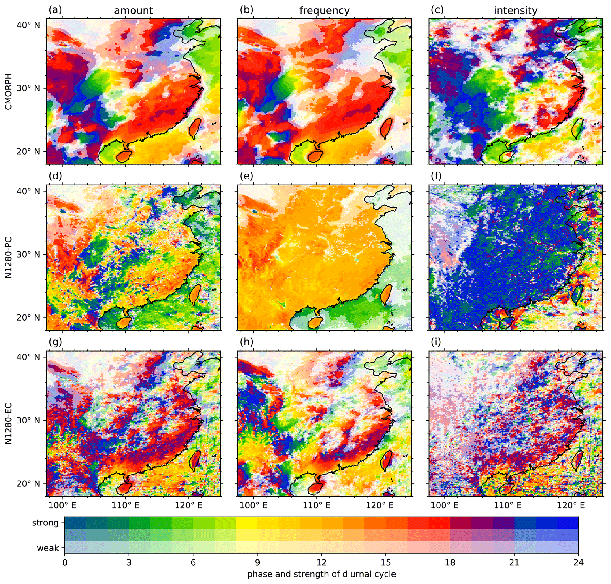
Figure 10Diurnal cycle of amount, frequency and precipitation over south-eastern China. Layout as in Fig. 9. A visual representation of the amplitude of the diurnal cycle is given by the opacity. This is calculated separately for each dataset over the entire Asian domain (Sect. 2.3), not for the subregion shown here.
As in Yu et al. (2007), their Fig. 3, and Chen et al. (2010), their Fig. 2a, a phase delay is also evident along 28∘ N, from 100 to 120∘ E for the diurnal cycle of the amount of precipitation. At the western end, the phase is in the late evening to midnight and the diurnal cycle is strong. Further east, between 107 and 113∘ E, the amplitude weakens and the phase is around 06:00–09:00 LST. At the eastern end, the phase is around 18:00 LST and the diurnal cycle is strong. There is a clear divide between the diurnal cycle over land and over ocean for all of amount, frequency and intensity, with oceanic precipitation peaking much closer to midday.
As in Sect. 3.3, N1280-PC produces a diurnal cycle of precipitation that is poorly matched with the observations across all three precipitation fields over both land and ocean. The frequency and intensity are both too uniform and generally have the wrong phase. For amount, there is more spatial variation, but the phase rarely matches that observed, being too close to midday. A phase delay at 28∘ N is difficult to discern.
N1280-EC bears a stronger resemblance to the observations for amount and frequency, although it produces too much late-night precipitation near the coast. The contrast between land and ocean is closer to the observed contrast than it is for N1280-PC. There are some signs of a phase delay going south-west to north-east across the Sichuan Basin, particularly in the frequency field, but it is not as clear as in the observations. This could be because N1280-EC produces too little precipitation in the Sichuan Basin (Fig. 9). Again, there is little clear sign of a phase delay at 28∘ N.
We can again compare directly with Li et al. (2018) and their Fig. 3. We note that they do not show the strength of the diurnal cycles. Comparing the observations, their diurnal cycles of amount and frequency of precipitation are similar, and so are those in this study. However, the phase of the peak is later over coastal China using CMORPH. This is consistent with Dai et al. (2007), who found that CMORPH had a delayed peak compared to gauge observations. Furthermore, the general patterns of amount, frequency and intensity are similar for both studies, although their fields are noisier (particularly frequency), which is to be expected given the shorter duration of their analysis.
Comparing the simulations to those of Li et al. (2018), the parametrized simulations produce diurnal cycles of amount, frequency and intensity that are very similar to each other (Fig. 10d, e and f here; their Fig. 3c, f and i). They see a slightly later peak in intensity in coastal China; however, this could be due to the particular year they have analysed or the boundary conditions provided by their coarser driving model. For the explicit simulations, more differences between this study and Li et al. (2018) are evident. Although both studies show a strong similarity between amount and frequency, the peak of the diurnal cycle of these often occurs later in this study over coastal regions than in Li et al. (2018). A similar comparison holds for intensity: there is a later peak in this study than in Li et al. (2018). Thus, even though both explicit simulations produce similar results for amount, frequency and intensity of precipitation (Sect. 4.1), this does not hold as strongly for their diurnal cycles. This could be due to the different resolutions, the shorter simulations or the boundary conditions they imposed on their regional model.
The value of aggregating precipitation over catchment basins was demonstrated in Schiemann et al. (2018). Here, we have extended that approach to allow for scale-selective analysis, which can be used to estimate the scales over which model simulations agree with observations and which is independent of the resolutions and grids of the datasets that are evaluated. This is similar in spirit to the fractional skill score metric (FSS), which can be used to determine the scale over which simulated precipitation is skilful (Roberts, 2008). However, there are important differences. For precipitation, the use of catchment basins provides a direct route into integrating the results from simulations into hydrological impact assessments, for example to predict large-scale flooding (e.g. Grams et al., 2014) or to provide useful information for the construction and management of dam networks (e.g. Zabalza-Martínez et al., 2018); these are not possible using the FSS. Furthermore, our approach could be used to provide a quantification of how the risks of widespread flooding or dams exceeding their limits will change due to a changing climate, in a way which takes into account the physical geography of a region.
We found that different configurations of a high-resolution GCM over Asia have some similar biases to coarser models. The biases are very similar when the same convection parametrization scheme is used, reinforcing the finding in e.g. Klingaman et al. (2017) and Martin et al. (2017) that this scheme is a key candidate for improving GCM performance. Disabling the scheme clearly produces a mean state that has larger biases than when it is enabled; however, the diurnal cycle of precipitation that is produced bears a stronger resemblance to the observational diurnal cycle. The high-resolution GCM configurations were not tuned, as the purpose is to compare the simulations on an equal footing following the CMIP6 HighResMIP philosophy (Haarsma et al., 2016). Given the mean biases identified in this study, some tuning of the N1280-resolution models will be necessary before using them in climatological and climate service applications.
The role of the convection parametrization scheme is clearly key in determining the spatial distribution, frequency, intensity and diurnal cycle of simulated precipitation. The scheme acts to remove convective instability by representing the bulk effect of the deep convective clouds in a grid column. The simulation that uses the scheme has more frequent precipitation and less intense precipitation compared to the explicit simulation (Fig. 9). The scheme uses a CAPE-based closure, which is non-local in the vertical (i.e. CAPE is an integral measure over the height of the atmosphere, and so the scheme can take into account the instability across the full height of a grid column). This is likely to be the reason why it produces more frequent precipitation; precipitation will occur when there is sufficient convective instability in a grid column (caused by, for example, surface heating, subsidence or radiative cooling). However, for the explicit simulation, convective precipitation will only be produced when the dynamics of the model react to local differences in convective instability. This can lead to a capping effect when there is sufficient convective inhibition (CIN). When the CIN is overcome (through, for example, orographic lifting), the built-up convective instability will be released. This is probably responsible for the increased intensity and reduced frequency of precipitation in the explicit simulation as well as for the improved timing of the diurnal cycle. Our results suggest that this capping effect is represented even at the comparatively coarse resolution of 14 km, although at this resolution the effect may be too strong. Further process-based analysis, testing the above suppositions, would be a worthwhile extension of the work here.
We note that the use of a convection parametrization scheme in our simulations is binary: it is either enabled or disabled for our fully parametrized and fully explicit simulations respectively. Given that this has such a large effect on the simulated precipitation, it difficult to ascertain the reasons for the differences between the simulations, as they are effectively at two ends of a spectrum. It could be beneficial to run a suite of experiments with the heating and moisture increments diagnosed by the scheme multiplied by different factors, e.g. 0 %, 25 %, 50 %, 75 % and 100 %. This would provide a more smoothly varying set of experiments, which would facilitate the analysis of the differences between the simulations. It may also provide some useful information on how to produce a scale-aware scheme – one which could be used at a range of different resolutions, blending seamlessly from fully parametrized to fully explicit convection. Thus, results from such experiments may provide useful insights for the development of scale-aware convection schemes such as CoMorph (Kendon et al., 2021).
The representation of simulated orographic precipitation seems to be particularly important (Sects. 3.1, 4.1 and 4.2); this has been noted in previous studies (Schiemann et al., 2018; Vannière et al., 2019) and is something we would like to investigate further. The nature of the precipitation is also important when considering the potential impacts: extreme convective precipitation increases the risk of landslides and localized flooding (He et al., 2018), whereas extreme large-scale precipitation increases the risk of widespread flooding and stresses dam networks (Hunt and Menon, 2020). It is likely that simulations with different configurations will have an effect on the distribution of precipitation; investigating this over catchment basins would be an interesting way to follow up our study.
Extending the simulation length would permit further analysis. Extremes of precipitation are difficult to analyse over only four summer seasons – with a longer duration more robust statistics on these could be generated, as in Schiemann et al. (2018). A longer simulation would also allow a better characterization of the climatology by sampling more interannual variability. However, previous works suggest that a longer simulation might not change the biases that we have identified, as the systematic errors which affect climate simulations develop after only a few days (Martin et al., 2010). The computational cost of such simulations would be high; however, the benefits would include an improved understanding of how various processes improve with increasing resolution and could also lay the foundations for the next generation of climate models.
Another way of producing high-resolution climate projections is by using statistical downscaling, as in Shashikanth et al. (2014), where they assess the utility of this method for projections of the ISM out to the 2080s. This method has the advantage of being less computationally demanding but drawbacks of not being able to represent smaller-scale features such as mesoscale convective systems and interactions between atmospheric flow and orography. Additionally, it assumes that statistical relationships that hold in the present-day climate will hold under a future climate, which may not be true. Thus, the high-resolution data generated by such methods may be useful for some applications but do not provide the same level of physical consistency as running high-resolution simulations.
We have compared the precipitation produced by new high-resolution GCM simulations against the observed precipitation from the CMORPH satellite dataset. The simulations were performed using the HadGEM3-GC3.1 Met Office Unified Model (UM) with a longitudinal grid length of 14 km at 30∘ N for 2005–2008. Three simulations were run: one with the standard UM convection parametrization scheme (N1280-PC), one with the deep convection scheme disabled but shallow and mid-level convection still parametrized (N1280-HC), and one where the convection scheme was disabled so convection was simulated explicitly by the model (N1280-EC). To determine the effect of resolution, we included results from other coarser-resolution HadGEM3-GC3.1 simulations, which also use the convection parametrization scheme.
6.1 Mean summer precipitation over Asia
We compared how the mean JJA precipitation over Asia was represented in the observations and simulations. We found that the simulations broadly reproduce observed Asian summer precipitation distribution. N1280-PC exhibited substantial biases compared with CMORPH, producing too much precipitation over the Indian Ocean, too little precipitation over India, and too much precipitation over south-eastern China. This is similar to biases seen in the UM at coarser resolutions; for example, Bush et al. (2015) found similar biases over India at N96 resolution. The N1280-PC simulation produced a band of precipitation on the Himalayas, indicating that it was representing some aspects of the interaction between the monsoon flow and orography, although the band was too wide and the precipitation rates were too high. The N1280-EC simulation worsened the existing biases in the UM, producing very little precipitation over India and maximum precipitation rates over the eastern end of the Himalayas that were far in excess of observations. The N1280-HC simulation performed similarly to N1280-EC over land.
Using the newly developed BASMATI, we averaged the precipitation field over hydrological catchment basins. The basins were chosen so that they were within a given size range, ranging from 2000–20 000 to 200 000–2 000 000 km2 for the small and large basin scales respectively. This allowed for the mean summer precipitation in the simulations to be compared against the observed precipitation from CMORPH as a function of spatial scale. We found that all the simulations improved as the spatial scale of analysis was increased and that the lowest-resolution simulation (N96-PC) produced the smallest error statistics, due mainly to its lack of very high precipitation rates.
6.2 Diurnal cycle of summer precipitation over Asia
Diurnal cycles of amount, frequency and intensity of precipitation were produced. We found that, for the summer diurnal cycle of precipitation over Asia, there were substantial differences between the observations and the simulations, with N1280-EC and N1280-HC generally performing far better than N1280-PC. For N1280-PC, the representation of the diurnal cycle is poor for all three precipitation measures. Over land across Asia, the peak in amount is too early at close to local midday, while the peak in frequency is too early at close to local midday and too uniform. The intensity is too late at local midnight and too uniform. For N1280-EC, the phase of the peak is more realistic for all three precipitation measures. However, the amplitude of the diurnal cycle is too weak over India, which we attributed to dry biases in this region. N1280-HC produced diurnal cycles that resemble both of the other simulations, yielding useful information about which aspect of the representation of convection is responsible for each of the diurnal cycles of amount, frequency and intensity. For the diurnal cycle of amount, N1280-HC closely resembles N1280-EC, indicating that the explicit deep convection is primarily responsible for producing this signal. For frequency, N1280-HC resembles N1280-PC more closely, indicating that the shallow and mid-level parametrizations of convection are responsible for this signal. However, in N1280-HC there is a clear difference between the diurnal cycles of amount and frequency, whereas in observations these fields are very similar.
Using BASMATI, diurnal cycles of amount, frequency and intensity were compared against CMORPH as a function of scale. For phase, N1280-EC and N1280-HC perform best for all three precipitation measures. These are the only simulations that perform better at a larger spatial scale for the amount of precipitation, which we attributed to their lack of a convection parametrization scheme. For the other simulations, higher resolution slightly improves the phase of the amount of precipitation. For the amplitude of amount, N1280-EC performs worst at small scales but improves more rapidly than the others as scale is increased, so that at the largest scales all the simulations perform similarly well. N1280-EC performs worst for intensity at all scales. The simulations which use a convection parametrization scheme at resolutions between N96 and N1280 (180 and 14 km grid length at 30∘ N respectively) perform almost identically and similarly poorly compared to CMORPH for frequency. This is consistent with the overestimation of precipitation frequency in parametrized simulations, as shown in Fig. 9 and e.g. Martin et al. (2017).
6.3 Summer precipitation over south-eastern China
Focusing on south-eastern China, the three precipitation measures in CMORPH matched similar analysis using gauge data in Li et al. (2018). The similarity was greatest for amount, which is least sensitive to the choice of threshold, whereas the frequency and intensity were generally lower and higher than those in Li et al. (2018) respectively. Li et al. (2018) used a regional version of the UM with both parametrized and explicit convection, and the explicit convection simulation had a finer resolution than the resolution used here. Similarly to Li et al. (2018), N1280-PC and N1280-EC overestimated the amount of precipitation, which we attributed to the overestimations of frequency for N1280-PC and to the overestimation of intensity for N1280-EC, consistent with Li et al. (2018). The similarities are apparent despite the differences in setup between this study and Li et al. (2018), which indicates that these are robust biases of the UM.
In N1280-PC, the land–sea contrast of the phase in maximum precipitation is unrealistic, whereas it is more realistic in N1280-EC. N1280-EC produces phase and amplitude for diurnal cycles of amount and frequency that are closer to the observed values, although the intensity is too weak.
6.4 Conclusions
The high-resolution global simulations we have analysed here show promise in representing some aspects of EASM precipitation despite producing large biases in the mean JJA precipitation. In particular, they reproduce the spatial patterns of the amount of precipitation over China reasonably well and compare well to similar regional models of the same area. The explicit-convection simulation produces a more realistic diurnal cycle than any parametrized-convection simulation. Further study of explicit-convection simulations, such as determining the scale at which they provide benefits over parametrized simulations, is likely to be beneficial. Additionally, development of scale-aware parametrizations, which seamlessly blend between fully parametrized at coarse resolution and fully explicit at fine resolution and take the best aspects of both representations of convection, would be highly desirable. However, some further work, some of which is already ongoing, will be necessary before HadGEM3 at N1280 resolution can be reliably used for climate projections:
-
tuning of the simulations to reduce the mean state precipitation bias;
-
longer simulations, which will allow for a better characterization of the climatology of the simulations;
-
process-based analysis, such as the ability of the simulations to represent mesoscale convective systems and the effect of orography; and
-
analysis of intraseasonal drivers of variability of the EASM, such as oscillations in the subtropical westerly jet and the boreal summer intraseasonal oscillation.
Furthermore, multiple model comparisons of high-resolution simulations such as Stevens et al. (2019) will be required before their full potential can be properly assessed. However, having a consistent representation of physics at all scales and the ability to reproduce regional and local precipitation patterns over Asian catchment basins would be invaluable for providing climate services to the region and determining the future hydrological changes expected from climate change.
The UM is available for use under licence. A number of research organisations and national meteorological services use the UM in collaboration with the Met Office to undertake basic atmospheric process research, produce forecasts, develop the UM code and build and evaluate Earth system models. For further information on how to apply for a licence, see https://www.metoffice.gov.uk/research/approach/collaboration/unified-model/partnership (Met Office, 2021).
The N1280 UM simulation output data are available upon request, as each simulation is over 80 TB in size and stored in the Met Office Managed Archive Storage System (MASS). The other simulations are part of CMIP6 HighResMIP and are available from the Earth System Grid Federation (ESGF) with DOIs as shown in https://www.primavera-h2020.eu/modelling/ (PRIMAVERA, 2021) and cited in Table 1, where N512-PC in this study refers to HadGEM3-GC31-HM, N216-PC refers to HadGEM3-GC31-MM, and N96-PC refers to HadGEM3-GC31-LM. All of these used the highresSST-present configuration.
CMORPH data are available from https://ftp.cpc.ncep.noaa.gov/precip/CMORPH_V1.0/CRT/8km-30min/ (NOAA, 2021).
The Basin-Scale Model Analysis ToolkIt (BASMATI) is freely available: https://doi.org/10.6084/m9.figshare.17049440.v1 (v0.3.3; Muetzelfeldt, 2021a).
The analysis packages that made use of BASMATI and produced all of the figures are also freely available: https://doi.org/10.6084/m9.figshare.17049428.v1 (v0.4.0 – Muetzelfeldt, 2021b) and https://doi.org/10.6084/m9.figshare.17206988.v1 (v0.4.1 – Muetzelfeldt, 2021c).
The supplement related to this article is available online at: https://doi.org/10.5194/hess-25-6381-2021-supplement.
Contributions by the different authors include conception of the study (MRM and RS), development of BASMATI, all data analysis and plotting of figures, and writing of the manuscript (MRM), performing the simulations (MJR and PLV), and feedback on the analysis as it progressed and on the manuscript (RS, NPK, AGT, PLV, MJR).
The contact author has declared that neither they nor their co-authors have any competing interests.
Publisher's note: Copernicus Publications remains neutral with regard to jurisdictional claims in published maps and institutional affiliations.
Mark R. Muetzelfeldt, Reinhard Schiemann, Andrew G. Turner, Nicholas P. Klingaman and Pier Luigi Vidale were supported by the COSMIC project through the Met Office Climate Science for Service Partnership (CSSP) China as part of the Newton Fund, contract number P106301. Nicholas P. Klingaman was supported by a Natural Environmental Research Council (NERC) Independent Research Fellowship (NE/L010976/1) and by the ACREW programme of the National Centre for Atmospheric Science. Malcolm J. Roberts received PRIMAVERA funding from the European Commission under grant agreement 641727 of the Horizon 2020 research programme.
The simulations were run using the Met Office supercomputer (https://www.metoffice.gov.uk/about-us/what/technology/supercomputer, last access: 15 December 2021), the ARCHER UK National Supercomputing Service (http://www.archer.ac.uk, last access: 15 December 2021), and MONSooN (https://www.metoffice.gov.uk/research/approach/collaboration/jwcrp/monsoon-hpc, last access: 15 December 2021). All analysis was done on JASMIN (https://www.jasmin.ac.uk/, last access: 15 December 2021).
This research has been supported by the Newton Fund (grant no. P106301), a NERC Independent Research Fellowship (NE/L010976/1), and the European Commission (grant agreement 641727).
This paper was edited by Rohini Kumar and reviewed by three anonymous referees.
Adler, R. F., Huffman, G. J., Chang, A., Ferraro, R., Xie, P.-P., Janowiak, J. E., Rudolf, B., Schneider, U., Curtis, S., Bolvin, D., Gruber, A., Susskind, J., Arkin, P., and Nelkin, E.: The Version-2 Global Precipitation Climatology Project (GPCP) Monthly Precipitation Analysis (1979–Present), J. Hydrometeorol., 4, 1147–1167, https://doi.org/10.1175/1525-7541(2003)004<1147:TVGPCP>2.0.CO;2, 2003. a
Ajayamohan, R. S., Rao, S. A., and Yamagata, T.: Influence of Indian Ocean dipole on poleward propagation of boreal summer intraseasonal oscillations, J. Climate, 21, 5437–5454, https://doi.org/10.1175/2008JCLI1758.1, 2008. a, b
Arakawa, A. and Schubert, W. H.: Interaction of a cumulus cloud ensemble with the large-scale environment, Part I, J. Atmos. Sci., 31, 674–701, https://doi.org/10.1175/1520-0469(1974)031<0674:IOACCE>2.0.CO;2, 1974. a
Bador, M., Boé, J., Terray, L., Alexander, L. V., Baker, A., Bellucci, A., Haarsma, R., Koenigk, T., Moine, M.-P., Lohmann, K., Putrasahan, D. A., Roberts, C., Roberts, M., Scoccimarro, E., Schiemann, R., Seddon, J., Senan, R., Valcke, S., and Vanniere, B.: Impact of higher spatial atmospheric resolution on precipitation extremes over land in global climate models, J. Geophys. Res.-Atmos., 125, e2019JD032184, https://doi.org/10.1029/2019JD032184, 2019. a
Bechtold, P., Semane, N., Lopez, P., Chaboureau, J.-P., Beljaars, A., and Bormann, N.: Representing equilibrium and nonequilibrium convection in large-scale models, J. Atmos. Sci., 71, 734–753, https://doi.org/10.1175/JAS-D-13-0163.1, 2014. a
Becker, T., Stevens, B., and Hohenegger, C.: Imprint of the convective parameterization and sea-surface temperature on large-scale convective self-aggregation, J. Adv. Model. Earth Syst., 9, 1488–1505, https://doi.org/10.1002/2016MS000865, 2017. a
Bollasina, M. A. and Ming, Y.: The general circulation model precipitation bias over the southwestern equatorial Indian Ocean and its implications for simulating the South Asian monsoon, Clim. Dynam., 40, 823–838, https://doi.org/10.1007/s00382-012-1347-7, 2013. a
Bougeault, P. and Geleyn, J. F.: Some problems of closure assumption and scale dependency in the parameterization of moist deep convection for numerical weather prediction, Meteorol. Atmos. Phys., 40, 123–135, 1989. a, b, c
Bush, S. J., Turner, A. G., Woolnough, S. J., Martin, G. M., and Klingaman, N. P.: The effect of increased convective entrainment on Asian monsoon biases in the MetUM general circulation model, Q. J. Roy. Meteorol. Soc., 141, 311–326, https://doi.org/10.1002/qj.2371, 2015. a, b, c, d
Chen, H., Yu, R., Li, J., Yuan, W., and Zhou, T.: Why nocturnal long-duration rainfall presents an eastward-delayed diurnal phase of rainfall down the Yangtze River valley, J. Climate, 23, 905–917, https://doi.org/10.1175/2009JCLI3187.1, 2010. a
Covey, C., Gleckler, P. J., Doutriaux, C., Williams, D. N., Dai, A., Fasullo, J., Trenberth, K. E., and Berg, A.: Metrics for the diurnal cycle of precipitation: Toward routine benchmarks for climate models, J. Climate, 29, 4461–4471, https://doi.org/10.1175/JCLI-D-15-0664.1, 2016. a, b, c, d
Curio, J., Chen, Y., Schiemann, R., Turner, A. G., Wong, K. C., Hodges, K., and Li, Y.: Comparison of a manual and an automated tracking method for Tibetan Plateau vortices, Adv. Atmos. Sci., 35, 965–980, https://doi.org/10.1007/s00376-018-7278-4, 2018. a
Dai, A. and Trenberth, K. E.: The diurnal cycle and its depiction in the Community Climate System Model, J. Climate, 17, 930–951, https://doi.org/10.1175/1520-0442(2004)017<0930:TDCAID>2.0.CO;2, 2004. a
Dai, A. and Wang, J.: Diurnal and semidiurnal tides in global surface pressure fields, J. Atmos. Sci., 56, 3874–3891, https://doi.org/10.1175/1520-0469(1999)056<3874:DASTIG>2.0.CO;2, 1999. a
Dai, A., Lin, X., and Hsu, K.-L.: The frequency, intensity, and diurnal cycle of precipitation in surface and satellite observations over low-and mid-latitudes, Clim. Dynam., 29, 727–744, https://doi.org/10.1007/s00382-007-0260-y, 2007. a, b
Ding, R., Ha, K.-J., and Li, J.: Interdecadal shift in the relationship between the East Asian summer monsoon and the tropical Indian Ocean, Clim. Dynam., 34, 1059–1071, https://doi.org/10.1007/s00382-009-0555-2, 2010. a
ESRI, E.: Shapefile technical description, An ESRI white paper, 39, available at: https://support.esri.com/en/white-paper/279 (last access: 15 December 2021), 1998. a
Field, P. R., Roberts, M. J., and Wilkinson, J. M.: Simulated lightning in a convection permitting global model, J. Geophys. Res.-Atmos., 123, 9370–9377, https://doi.org/10.1029/2018JD029295, 2018. a, b, c
Golding, B. W.: Quantitative precipitation forecasting in the UK, J. Hydrol., 239, 286–305, https://doi.org/10.1016/S0022-1694(00)00354-1, 2000. a
Grams, C. M., Binder, H., Pfahl, S., Piaget, N., and Wernli, H.: Atmospheric processes triggering the central European floods in June 2013, Nat. Hazards Earth Syst. Sci., 14, 1691–1702, https://doi.org/10.5194/nhess-14-1691-2014, 2014. a
Haarsma, R. J., Roberts, M. J., Vidale, P. L., Senior, C. A., Bellucci, A., Bao, Q., Chang, P., Corti, S., Fučkar, N. S., Guemas, V., von Hardenberg, J., Hazeleger, W., Kodama, C., Koenigk, T., Leung, L. R., Lu, J., Luo, J.-J., Mao, J., Mizielinski, M. S., Mizuta, R., Nobre, P., Satoh, M., Scoccimarro, E., Semmler, T., Small, J., and von Storch, J.-S.: High Resolution Model Intercomparison Project (HighResMIP v1.0) for CMIP6, Geosci. Model Dev., 9, 4185–4208, https://doi.org/10.5194/gmd-9-4185-2016, 2016. a, b, c, d, e, f
He, B., Huang, X., Ma, M., Chang, Q., Tu, Y., Li, Q., Zhang, K., and Hong, Y.: Analysis of flash flood disaster characteristics in China from 2011 to 2015, Nat. Hazards, 90, 407–420, https://doi.org/10.1007/s11069-017-3052-7, 2018. a
Holloway, C. E., Woolnough, S. J., and Lister, G. M. S.: The effects of explicit versus parameterized convection on the MJO in a large-domain high-resolution tropical case study. Part I: Characterization of large-scale organization and propagation, J. Atmos. Sci., 70, 1342–1369, https://doi.org/10.1175/JAS-D-12-0227.1, 2013. a
Houze Jr., R. A.: Mesoscale convective systems, Rev. Geophys., 42, RG4003, https://doi.org/10.1029/2004RG000150, 2004. a
Hsu, P.-C., Lee, J.-Y., and Ha, K.-J.: Influence of boreal summer intraseasonal oscillation on rainfall extremes in southern China, Int. J. Climatol., 36, 1403–1412, https://doi.org/10.1002/joc.4433, 2016. a
Hunt, K. M. and Menon, A.: The 2018 Kerala floods: a climate change perspective, Clim. Dynam., 54, 2433–2446, https://doi.org/10.1007/s00382-020-05123-7, 2020. a
Hurkmans, R., Terink, W., Uijlenhoet, R., Torfs, P., Jacob, D., and Troch, P. A.: Changes in streamflow dynamics in the Rhine basin under three high-resolution regional climate scenarios, J. Climate, 23, 679–699, https://doi.org/10.1175/2009JCLI3066.1, 2010. a, b
Joyce, R. J., Janowiak, J. E., Arkin, P. A., and Xie, P.: CMORPH: A method that produces global precipitation estimates from passive microwave and infrared data at high spatial and temporal resolution, J. Hydrometeorol., 5, 487–503, https://doi.org/10.1175/1525-7541(2004)005<0487:CAMTPG>2.0.CO;2, 2004. a, b, c
Kendon, E. J., Prein, A. F., Senior, C. A., and Stirling, A.: Challenges and outlook for convection-permitting climate modelling, Philos. T. Roy. Soc. A, 379, 20190547, https://doi.org/10.1098/rsta.2019.0547, 2021. a
Kennedy, J., Titchner, H., Rayner, N., and Roberts, M. J.: input4MIPs.MOHC.SSTsAndSeaIce.HighResMIP.MOHC-HadISST-2-2-0-0-0, Earth System Grid Federation, UK Met Office, https://doi.org/10.22033/ESGF/input4MIPs.1221, 2017. a
Khairoutdinov, M., Randall, D., and DeMott, C.: Simulations of the atmospheric general circulation using a cloud-resolving model as a superparameterization of physical processes, J. Atmos. Sci., 62, 2136–2154, https://doi.org/10.1175/JAS3453.1, 2005. a
Klingaman, N. P., Martin, G. M., and Moise, A. F.: ASoP (v1.0): A set of methods for analyzing scales of precipitation in general circulation models, Geosci. Model Dev., 10, 57–83, https://doi.org/10.5194/gmd-10-57-2017, 2017. a, b, c
Lehner, B.: HydroBASINS: Global watershed boundaries and sub-basin delineations derived from HydroSHEDS data at 15 second resolution, Technical Documentation Version 1.c (with and without inserted lakes), available at: https://hydrosheds.org/images/inpages/HydroBASINS_TechDoc_v1c.pdf (last access: 15 December 2021), 2014. a
Lehner, B. and Grill, G.: Global river hydrography and network routing: baseline data and new approaches to study the world's large river systems, Hydrol. Process., 27, 2171–2186, https://doi.org/10.1002/hyp.9740, 2013. a, b
Levine, R. C., Turner, A. G., Marathayil, D., and Martin, G. M.: The role of northern Arabian Sea surface temperature biases in CMIP5 model simulations and future projections of Indian summer monsoon rainfall, Clim. Dynam., 41, 155–172, https://doi.org/10.1007/s00382-012-1656-x, 2013. a
Li, J., Li, Y., Zhao, T., Schiemann, R., Jiang, X., and Muetzelfeldt, M.: Northeastward propagation of nocturnal precipitation over the Sichuan Basin, Int. J. Climatol., 41, E2863–E2879, https://doi.org/10.1002/joc.6886, 2020. a, b
Li, P., Furtado, K., Zhou, T., Chen, H., Li, J., Guo, Z., and Xiao, C.: The diurnal cycle of East Asian summer monsoon precipitation simulated by the Met Office Unified Model at convection-permitting scales, Clim. Dynam., 55, 131–151, https://doi.org/10.1007/s00382-018-4368-z, 2018. a, b, c, d, e, f, g, h, i, j, k, l, m, n, o, p, q, r, s, t, u, v, w, x, y, z
Marsham, J. H., Dixon, N. S., Garcia-Carreras, L., Lister, G. M. S., Parker, D. J., Knippertz, P., and Birch, C. E.: The role of moist convection in the West African monsoon system: Insights from continental-scale convection-permitting simulations, Geophys. Res. Lett., 40, 1843–1849, https://doi.org/10.1002/grl.50347, 2013. a, b, c
Martin, G. M., Milton, S. F., Senior, C. A., Brooks, M. E., Ineson, S., Reichler, T., and Kim, J.: Analysis and reduction of systematic errors through a seamless approach to modeling weather and climate, J. Climate, 23, 5933–5957, https://doi.org/10.1175/2010JCLI3541.1, 2010. a
Martin, G. M., Klingaman, N. P., and Moise, A. F.: Connecting spatial and temporal scales of tropical precipitation in observations and the MetUM-GA6, Geosci. Model Dev., 10, 105–126, https://doi.org/10.5194/gmd-10-105-2017, 2017. a, b, c, d
Met Office: Unified Model Partnership, available at: https://www.metoffice.gov.uk/research/approach/collaboration/unified-model/partnership, last access: 15 December 2021. a
Mitra, A. K., Momin, I. M., Rajagopal, E. N., Basu, S., Rajeevan, M. N., and Krishnamurti, T. N.: Gridded daily Indian monsoon rainfall for 14 seasons: Merged TRMM and IMD gauge analyzed values, J. Earth Syst. Sci., 122, 1173–1182, https://doi.org/10.1007/s12040-013-0338-3, 2013. a
Muetzelfeldt, M. R.: basmati, figshare [code], https://doi.org/10.6084/m9.figshare.17049440.v1, 2021a. a
Muetzelfeldt, M. R.: Muetzelfeldt, M. R.: cosmic, figshare [code], https://doi.org/10.6084/m9.figshare.17049428.v1, 2021b. a
Muetzelfeldt, M. R.: remake_v0.4.1, figshare [code], https://doi.org/10.6084/m9.figshare.17206988.v1, 2021c. a
Mulcahy, J. P., Jones, C., Sellar, A., Johnson, B., Boutle, I. A., Jones, A., Andrews, T., Rumbold, S. T., Mollard, J., Bellouin, N., Johnson, C. E., Williams, K. D., Grosvenor, D. P., and McCoy, D. T.: Improved aerosol processes and effective radiative forcing in HadGEM3 and UKESM1, J. Adv. Model. Earth Syst., 10, 2786–2805, https://doi.org/10.1029/2018MS001464, 2018. a
NOAA: Index of /precip/CMORPH_V1.0/CRT/8km-30min, NOAA [data set], https://ftp.cpc.ncep.noaa.gov/precip/CMORPH_V1.0/CRT/8km-30min/, last access: 15 December 2021. a
Ploshay, J. J. and Lau, N.-C.: Simulation of the diurnal cycle in tropical rainfall and circulation during boreal summer with a high-resolution GCM, Mon. Weather Rev., 138, 3434–3453, https://doi.org/10.1175/2010MWR3291.1, 2010. a
PRIMAVERA: Climate model simulations, PRIMAVERA [code], https://www.primavera-h2020.eu/modelling/, last access: 15 December 2021. a
Reichle, R. H., Koster, R. D., De Lannoy, G. J. M., Forman, B. A., Liu, Q., Mahanama, S. P. P., and Touré, A.: Assessment and enhancement of MERRA land surface hydrology estimates, J. Climate, 24, 6322–6338, https://doi.org/10.1175/JCLI-D-10-05033.1, 2011. a
Roberts, M. J.: MOHC HadGEM3-GC31-HM model output prepared for CMIP6 HighResMIP, Earth System Grid Federation, Met Office, https://doi.org/10.22033/ESGF/CMIP6.446, 2017a. a
Roberts, M. J.: MOHC HadGEM3-GC31-LM model output prepared for CMIP6 HighResMIP, Earth System Grid Federation, Met Office, https://doi.org/10.22033/ESGF/CMIP6.1321, 2017b. a
Roberts, M. J.: MOHC HadGEM3-GC31-MM model output prepared for CMIP6 HighResMIP, Earth System Grid Federation, Met Office, https://doi.org/10.22033/ESGF/CMIP6.1902, 2017c. a
Roberts, M. J., Vidale, P. L., Senior, C., Hewitt, H. T., Bates, C., Berthou, S., Chang, P., Christensen, H. M., Danilov, S., Demory, M.-E., Griffies, S. M., Haarsma, R., Jung, T., Martin, G., Minobe, S., Ringler, T., Satoh, M., Schiemann, R., Scoccimarro, E., Stephens, G., and Wehner, M. F.: The benefits of global high resolution for climate simulation: process understanding and the enabling of stakeholder decisions at the regional scale, B. Am. Meteorol. Soc., 99, 2341–2359, https://doi.org/10.1175/BAMS-D-15-00320.1, 2018. a
Roberts, M. J., Baker, A., Blockley, E. W., Calvert, D., Coward, A., Hewitt, H. T., Jackson, L. C., Kuhlbrodt, T., Mathiot, P., Roberts, C. D., Schiemann, R., Seddon, J., Vannière, B., and Vidale, P. L.: Description of the resolution hierarchy of the global coupled HadGEM3-GC3.1 model as used in CMIP6 HighResMIP experiments, Geosci. Model Dev., 12, 4999–5028, https://doi.org/10.5194/gmd-12-4999-2019, 2019. a, b, c, d
Roberts, N.: Assessing the spatial and temporal variation in the skill of precipitation forecasts from an NWP model, Meteorol. Appl., 15, 163–169, https://doi.org/10.1002/met.57, 2008. a
Sato, T., Miura, H., Satoh, M., Takayabu, Y. N., and Wang, Y.: Diurnal cycle of precipitation in the tropics simulated in a global cloud-resolving model, J. Climate, 22, 4809–4826, https://doi.org/10.1175/2009JCLI2890.1, 2009. a
Satoh, M., Tomita, H., Yashiro, H., Miura, H., Kodama, C., Seiki, T., Noda, A. T., Yamada, Y., Goto, D., Sawada, M., Miyoshi, T., Niwa, Y., Hara, M., Ohno, T., Iga, S.-I., Arakawa, T., Inoue, T., and Kubokawa, H.: The non-hydrostatic icosahedral atmospheric model: Description and development, Progr. Earth Planet. Sci., 1, 18, https://doi.org/10.1186/s40645-014-0018-1, 2014. a
Schär, C., Fuhrer, O., Arteaga, A., Ban, N., Charpilloz, C., Di Girolamo, S., Hentgen, L., Hoefler, T., Lapillonne, X., Leutwyler, D., Osterried, K., Panosetti, D., Rüdisühli, S., Schlemmer, L., Schulthess, T. C., Sprenger, M., Ubbiali, S., and Wernli, H.: Kilometer-scale climate models: Prospects and challenges, B. Am. Meteorol. Soc., 101, E567–E587, https://doi.org/10.1175/BAMS-D-18-0167.1, 2020. a
Schiemann, R., Vidale, P. L., Shaffrey, L. C., Johnson, S. J., Roberts, M. J., Demory, M.-E., Mizielinski, M. S., and Strachan, J.: Mean and extreme precipitation over European river basins better simulated in a 25 km AGCM, Hydrol. Earth Syst. Sci., 22, 3933–3950, https://doi.org/10.5194/hess-22-3933-2018, 2018. a, b, c, d, e, f
Shashikanth, K., Madhusoodhanan, C. G., Ghosh, S., Eldho, T. I., Rajendran, K., and Murtugudde, R.: Comparing statistically downscaled simulations of Indian monsoon at different spatial resolutions, J. Hydrol., 519, 3163–3177, 2014. a
Sheffield, J., Goteti, G., and Wood, E. F.: Development of a 50-year high-resolution global dataset of meteorological forcings for land surface modeling, J. Climate, 19, 3088–3111, https://doi.org/10.1175/JCLI3790.1, 2006. a
Smagorinsky, J.: Some aspects of the general circulation, Q. J. Roy. Meteorol. Soc., 90, 1–14, https://doi.org/10.1002/qj.49709038302, 1964. a
Stevens, B., Fiedler, S., Kinne, S., Peters, K., Rast, S., Müsse, J., Smith, S. J., and Mauritsen, T.: MACv2-SP: A parameterization of anthropogenic aerosol optical properties and an associated Twomey effect for use in CMIP6, Geosci. Model Dev., 10, 433–452, https://doi.org/10.5194/gmd-10-433-2017, 2017. a, b
Stevens, B., Satoh, M., Auger, L., Biercamp, J., Bretherton, C. S., Chen, X., Düben, P., Judt, F., Khairoutdinov, M., Klocke, D., Kodama, C., Kornblueh, L., Lin, S.-J., Neumann, P., Putman, W. M., Röber, N., Shibuya, R., Vanniere, B., Vidale, P. L., Wedi, N., and Zhou, L.: DYAMOND: the DYnamics of the Atmospheric General Circulation Modeled On Non-hydrostatic Domains, Progr. Earth Planet. Sci., 6, 1–17, 2019. a
Stirling, A. J. and Stratton, R. A.: Entrainment processes in the diurnal cycle of deep convection over land, Q. J. Roy. Meteorol. Soc., 138, 1135–1149, https://doi.org/10.1002/qj.1868, 2012. a, b
Titchner, H. A. and Rayner, N. A.: The Met Office Hadley Centre sea ice and sea surface temperature data set, version 2: 1. Sea ice concentrations, J. Geophys. Res.-Atmos., 119, 2864–2889, https://doi.org/10.1002/2013JD020316, 2014. a
Tomassini, L.: Mesoscale circulations and organized convection in African easterly waves, J. Atmos. Sci., 75, 4357–4381, https://doi.org/10.1175/JAS-D-18-0183.1, 2018. a
Vannière, B., Demory, M.-E., Vidale, P. L., Schiemann, R., Roberts, M. J., Roberts, C. D., Matsueda, M., Terray, L., Koenigk, T., and Senan, R.: Multi-model evaluation of the sensitivity of the global energy budget and hydrological cycle to resolution, Clim. Dynam., 52, 6817–6846, https://doi.org/10.1007/s00382-018-4547-y, 2019. a, b, c, d
Verdin, K. L. and Verdin, J. P.: A topological system for delineation and codification of the Earth's river basins, J. Hydrol., 218, 1–12, https://doi.org/10.1016/S0022-1694(99)00011-6, 1999. a, b
Vergara-Temprado, J., Ban, N., Panosetti, D., Schlemmer, L., and Schär, C.: Climate Models Permit Convection at Much Coarser Resolutions Than Previously Considered, J. Climate, 33, 1915–1933, https://doi.org/10.1175/JCLI-D-19-0286.1, 2020. a
Virts, K. S. and Houze Jr., R. A.: Seasonal and intraseasonal variability of mesoscale convective systems over the South Asian monsoon region, J. Atmos. Sci., 73, 4753–4774, https://doi.org/10.1175/JAS-D-16-0022.1, 2016. a
Walters, D., Boutle, I., Brooks, M., Melvin, T., Stratton, R., Vosper, S., Wells, H., Williams, K., Wood, N., Allen, T., Bushell, A., Copsey, D., Earnshaw, P., Edwards, J., Gross, M., Hardiman, S., Harris, C., Heming, J., Klingaman, N., Levine, R., Manners, J., Martin, G., Milton, S., Mittermaier, M., Morcrette, C., Riddick, T., Roberts, M., Sanchez, C., Selwood, P., Stirling, A., Smith, C., Suri, D., Tennant, W., Vidale, P. L., Wilkinson, J., Willett, M., Woolnough, S., and Xavier, P.: The Met Office Unified Model Global Atmosphere 6.0/6.1 and JULES Global Land 6.0/6.1 configurations, Geosci. Model Dev., 10, 1487–1520, https://doi.org/10.5194/gmd-10-1487-2017, 2017. a
Walters, D., Baran, A. J., Boutle, I., Brooks, M., Earnshaw, P., Edwards, J., Furtado, K., Hill, P., Lock, A. P., Manners, J., Morcrette, C., Mulcahy, J., Sanchez, C., Smith, C., Stratton, R. A., Tennant, W. J., Tomassini, L., Van Weverberg, K., Vosper, S., Willett, M. R., Browse, J., Bushell, A., Carslaw, K., Dalvi, M., Essery, R., Gedney, N., Hardiman, S., Johnson, B., Johnson, C., Jones, A., Jones, C., Mann, G., Milton, S., Rumbold, H., Sellar, A., Ujiie, M., Whitall, M. A., Williams, K., and Zerroukat, M.: The Met Office Unified Model Global Atmosphere 7.0/7.1 and JULES Global Land 7.0 configurations, Geosci. Model Dev., 12, 1909–1963, https://doi.org/10.5194/gmd-12-1909-2019, 2019. a, b
Webb, M. J., Lock, A. P., Bretherton, C. S., Bony, S., Cole, J. N. S., Idelkadi, A., Kang, S. M., Koshiro, T., Kawai, H., Ogura, T., Roehrig, R., Shin, Y., Mauritsen, T., Sherwood, S. C., Vial, J., Watanabe, M., Woelfle, M. D., and Zhao, M.: The impact of parametrized convection on cloud feedback, Philos. T. Roy. Soc. A, 373, 20140414, https://doi.org/10.1098/rsta.2014.0414, 2015. a
Willetts, P. D., Marsham, J. H., Birch, C. E., Parker, D. J., Webster, S., and Petch, J.: Moist convection and its upscale effects in simulations of the Indian monsoon with explicit and parametrized convection, Q. J. Roy. Meteorol. Soc., 143, 1073–1085, https://doi.org/10.1002/qj.2991, 2017. a, b, c
Williams, K. D., Copsey, D., Blockley, E. W., Bodas-Salcedo, A., Calvert, D., Comer, R., Davis, P., Graham, T., Hewitt, H. T., Hill, R., Hyder, P., Ineson, S., Johns, T. C., Keen, A. B., Lee, R. W., Megann, A., Milton, S. F., Rae, J. G. L., Roberts, M. J., Scaife, A. A., Schiemann, R., Storkey, D., Thorpe, L., Watterson, I. G., Walters, D. N., West, A., Wood, R. A., Woollings, T., and Xavier, P. K.: The Met Office global coupled model 3.0 and 3.1 (GC3.0 and GC3.1) configurations, J. Adv. Model. Earth Syst., 10, 357–380, https://doi.org/10.1002/2017MS001115, 2018. a
Wu, R. and Wang, B.: A contrast of the East Asian summer monsoon–ENSO relationship between 1962–77 and 1978–93, J. Climate, 15, 3266–3279, https://doi.org/10.1175/1520-0442(2002)015<3266:ACOTEA>2.0.CO;2, 2002. a
Xavier, P. K., Marzin, C., and Goswami, B. N.: An objective definition of the Indian summer monsoon season and a new perspective on the ENSO–monsoon relationship, Q. J. Roy. Meteorol. Soc., 133, 749–764, https://doi.org/10.1002/qj.45, 2007. a
Yang, G.-Y. and Slingo, J.: The diurnal cycle in the tropics, Mon. Weather Rev., 129, 784–801, https://doi.org/10.1175/1520-0493(2001)129<0784:TDCITT>2.0.CO;2, 2001. a, b, c
Yang, X., Fei, J., Huang, X., Cheng, X., Carvalho, L. M. V., and He, H.: Characteristics of mesoscale convective systems over China and its vicinity using geostationary satellite FY2, J. Climate, 28, 4890–4907, https://doi.org/10.1175/JCLI-D-14-00491.1, 2015. a
Yatagai, A., Kamiguchi, K., Arakawa, O., Hamada, A., Yasutomi, N., and Kitoh, A.: APHRODITE: Constructing a long-term daily gridded precipitation dataset for Asia based on a dense network of rain gauges, B. Am. Meteorol. Soc., 93, 1401–1415, https://doi.org/10.1175/BAMS-D-11-00122.1, 2012. a
Yu, R., Zhou, T., Xiong, A., Zhu, Y., and Li, J.: Diurnal variations of summer precipitation over contiguous China, Geophys. Res. Lett., 34, L01704, https://doi.org/10.1029/2006GL028129, 2007. a
Zabalza-Martínez, J., Vicente-Serrano, S. M., López-Moreno, J. I., Borràs Calvo, G., Savé, R., Pascual, D., Plá, E., Morán-Tejeda, E., Domínguez-Castro, F., and Tague, C.: The Influence of Climate and Land-Cover Scenarios on Dam Management Strategies in a High Water Pressure Catchment in Northeast Spain, Water, 10, 1668, https://doi.org/10.3390/w10111668, 2018. a
Zhang, L., Wu, P., Zhou, T., Roberts, M. J., and Schiemann, R.: Added value of high resolution models in simulating global precipitation characteristics, Atmos. Sci. Lett., 17, 646–657, https://doi.org/10.1002/asl.715, 2016. a
Zhang, Q., Gu, X., Li, J., Shi, P., and Singh, V. P.: The impact of tropical cyclones on extreme precipitation over coastal and inland areas of China and its association to ENSO, J. Climate, 31, 1865–1880, https://doi.org/10.1175/JCLI-D-17-0474.1, 2018. a
Zhong, Z. and Hu, Y.: Impacts of tropical cyclones on the regional climate: An East Asian summer monsoon case, Atmos. Sci. Lett., 8, 93–99, https://doi.org/10.1002/asl.158, 2007. a
Zhou, T., Yu, R., Chen, H., Dai, A., and Pan, Y.: Summer precipitation frequency, intensity, and diurnal cycle over China: A comparison of satellite data with rain gauge observations, J. Climate, 21, 3997–4010, https://doi.org/10.1175/2008JCLI2028.1, 2008. a, b
- Abstract
- Copyright statement
- Introduction
- Data and methods
- Precipitation over Asia
- Precipitation over south-eastern China
- Discussion
- Summary and conclusions
- Code and data availability
- Author contributions
- Competing interests
- Disclaimer
- Acknowledgements
- Financial support
- Review statement
- References
- Supplement