Identification of the contributing area to river discharge during low-flow periods

The increasing severity of hydrological droughts in the Mediterranean basin related to climate change raises the need to understand the processes sustaining low flow. The purpose of this paper is to evaluate simple mixing model approaches, first to identify and then to quantify streamflow contribution during low-water periods. An approach based on the coupling of geochemical data with hydrological data allows the quantification of flow contributions. In addition, monitoring during the low-water period was used to investigate the drying-up trajectory of each geological reservoir individually. Data were collected during the summers of 2018 and 2019 on a Mediterranean river (Gardon de Sainte-Croix). The identification of the end-members was performed after the identification of a groundwater geochemical signature clustered according to the geological nature of the reservoir. Two complementary methods validate further the characterisation: rock-leaching experiments and unsupervised classification (k-means). The use of the end-member mixture analysis (EMMA) coupled with a generalised likelihood uncertainty estimate (GLUE) (G-EMMA) mixing model coupled with hydrological monitoring of the main river discharge rate highlights major disparities in the contribution of the geological units, showing a reservoir with a minor contribution in high flow becoming preponderant during the low-flow period. This finding was revealed to be of the utmost importance for the management of water resources during the dry period.

1 Introduction

An increase in the severity of hydrological droughts, in terms of both duration and intensity found to be related to climate change, has been observed in the Mediterranean basin (Aubé, 2017; Bard et al., 2012; Giuntoli et al., 2015; Marx et al., 2018; Ruiz-Villanueva et al., 2014; Sauquet et al., 2015; Van Vliet et al., 2013; Vidal et al., 2016). The increase in the severity of low-water levels contributes to degrading the water resources in terms of both quantity and quality (Nosrati, 2011; Chiogna et al., 2018), thus impacting ecosystems connected to the river (Folegot et al., 2018). This trend enhances the need for a better understanding of the hydrological processes during these periods of resource scarcity (Buytaert et al., 2006; Chiogna et al., 2018; Correa et al., 2017). Investigations on the processes that sustain streamflow have been identified as a requirement for understanding the dynamics of the hydrological system (Smakhtin, 2001). Hence, as a first step, identifying the origin of the water that feeds streamflow during low-water episodes is essential.

The approach often used in the study of low flows targets the contribution dynamics of the different units of the watershed during those periods (Blumstock et al., 2015; Cartwright and Morgenstern, 2012; Cook et al., 2006) by focusing on the differences in contributions amongst the major units of the watershed, i.e. shallow groundwater, deep groundwater, rainfall, and sub-surface, or on the exchanges with the water table in lowland areas (Petelet-Giraud et al., 2018; Blumstock et al., 2016). Many studies emphasise the predominance of groundwater in maintaining flows in mountain areas (Tetzlaff and Soulsby, 2008) and more generally in maintaining baseflow. It is also commonly accepted that the process of baseflow generation is controlled by the nature of the geology of the watershed (Bloomfield et al., 2009; Farvolden, 1963; Freeze and Cherry, 1979; Neff et al., 2005; Smakhtin, 2001; Tague and Grant, 2004). Some studies investigated the origin of water in a stream based on the geological nature of the reservoir during high flow (Petelet-Giraud et al., 2018; Floriancic et al., 2018), but this has rarely been applied to low flow. The aim of this study was, therefore, to identify and then quantify the contributions of the different geological reservoirs during low-water conditions in a watershed showing a variety of geological facies.

The methods usually used to investigate the origin of water commonly conceptualise catchment areas in different landscape entities with specific geochemical signatures and then unravel each reservoir contribution using hydrogeochemical mixing models, such as the end-member mixture analysis (EMMA) (Christophersen and Hooper, 1992; Ali et al., 2010; Correa et al., 2017; Inamdar et al., 2013; Hooper, 2001). This approach considers the hydrogeochemical composition of the river water to be the result of the mixture of the different reservoirs contributing to the flow (Christophersen et al., 1990). Assumptions about conservative behaviour and linear mixing process are both equally necessary to run mixing models (Hooper, 2001). The contribution of each end-member is identified by tracing all potential water contribution to the streamflow, selected according to their ability to represent the overall variability of the geochemical signature of the stream data (Levia, 2011). The main interest of the EMMA analysis resides in its ability to consider the whole dispersion of the tracers and thus consider all possible mixing configurations associated with their output probabilities in the runs of the model (Barthold et al., 2017, 2011). With this tool, hydrogeochemical information is particularly valuable when used in combination with hydrometric data (Buttle, 1994; Inamdar et al., 2013). The use of this model with geochemical and hydrological data permits the decomposition of the discharge in several ways. It is thus possible to quantify the proportion of water coming from different seasonal recharges or to quantify the proportion coming from different units of the discharge (Ali et al., 2010; Correa et al., 2017; Delsman et al., 2013; Inamdar and Mitchell, 2007; Inamdar et al., 2013; Morel et al., 2009). Model uncertainties are assessed based on the propagation of Gaussian errors (Genereux, 1998; Phillips and Gregg, 2001). Uncertainties in the contribution estimation obtained with these models can only be minimised if the assumptions made for these tools (use of non-reactive tracer and marked difference in the end-member) are followed (Barthold et al., 2011). Estimates of the contribution of each end-member depend on tracers (Genereux, 1998), their numbers (Barthold et al., 2011), measurement uncertainties (Bazemore et al., 1994; Genereux, 1998) and the number of end-members included in the analysis (Delsman et al., 2013).

The majority of the studies using EMMA analyses focus on the identification of water during flood peaks (Brown et al., 1999; Burns et al., 2001; Engel et al., 2016; Evans and Davies, 1998; Fröhlich et al., 2008; Lloyd et al., 2016; Tetzlaff et al., 2014; Tunaley et al., 2017; Yang et al., 2015). Some authors also worked on the whole hydrological year (Correa et al., 2019; Petelet-Giraud et al., 2018, 2016; Petelet-Giraud and Negrel, 2007), but the focus generally remains on floods rather than on low flows. Most studies conceptualise water catchments into several major components: deep groundwaters, shallow groundwaters, soil water and rainwater. By focusing only on the low-water period in a watershed where the alluvial water table is limited, it is possible to consider the contribution of groundwaters and differentiate the reservoirs according to their geology. This paper shows the applicability of the EMMA method for identifying the origin of surface water during low flow to understand flow dynamics in catchments during periods of scarcity. This will provide a better understanding of the behaviour of this watershed during low-flow periods and allow the identification of reservoirs offering the highest runoff-generation contribution, which will ultimately allow improvement in resource management by concentrating protection on these reservoirs.

This approach of dealing exclusively with low-water levels is of interest as, although the application of these methods is frequent in hydrology, it is rarely applied during low flow. The water contribution of each groundwater reservoir feeding the mainstream during the drying period will, first, be identified based on the geochemical properties of the reservoir and, second, be quantified. Then the drying-out curve of each of the reservoirs will be computed. Hence, in the present paper, we intend to identify the geological reservoirs contributing to river flows and then to quantify their respective contributions during low flow. Two strong assumptions are made: an exclusive origin of low-flow waters from groundwater and possible discrimination of the end-member geochemical signatures related to their geological formation. The proposed approach is applied to a real case study. In order to take into account the limitations raised in the use of EMMA, include the assumption of the conservative behaviour of the end-member tracers in the model and fulfil the need to implement an unbiased method to define the end-members in terms of their number and the accuracy of their signatures, the approach presented will combine different tools (Barthold et al., 2011; James and Roulet, 2006; Hooper, 2001, 2003). To take into account this limitation, our approach will include statistical classification, a leaching approach and a multiple definition of the end-member signature. This combined approach will limit the problems of this geochemical modelling. Moreover, focusing on this period and not on the whole hydrological year facilitates a higher sampling rate and provides a finer analysis of the reservoirs' drying-up mechanisms feeding the river (Floriancic et al., 2018).

The article is organized into three sections. The first presents the watershed studied and the methodology proposed to identify the groundwater end-members in terms of the geological nature of the reservoir, and it then quantifies their contributions. The second section describes the results obtained in identifying the end-members and in the contributions produced by the mixing models, whilst the third section provides a discussion on the followed methodology and results.

2 Methodology

This study aims to differentiate, during the low-flow period, the origin of surface water according to the geological nature of the contributing reservoir. This approach is based on the assumption that only groundwater supplies streamflow during low-flow periods. This allows us to exclude rainwater from the process and disregard these reservoirs, letting us limit the number of contributing reservoirs, thus minimising the dispersion of our approach. The methodology relies first on the identification of different hydrogeochemical end-members present in the study area. These identified hydrogeochemical end-members are then linked to the different geological formations. Finally, a weekly hydrogeochemical survey of groundwater and surface water during the summer allowed us to quantify the contributions of each reservoir to surface water.

2.1 Study area

The study area is located in the south of France, in the Cévennes region, a Mediterranean mountainous chain 100 km north of Montpellier (see Fig. 1). Our approach was developed on the Gardon de Sainte-Croix watershed, which has an area of 95 km². This watershed located in the Cévennes area has a relatively simple geology, with three dominant geological units and limited anthropisation, which facilitate geochemical analyses and interpretation. The climate in the studied region is defined as Mediterranean with a very high annual rainfall of 1110 mm on average per year (Barre-des-Cévennes rain recorder, 1981 to 2010, Météo-France, denoted as BC in Fig. 1). Although total rainfall is high, summer rainfall is very low, less than 50 mm (July to September), and almost half of the total annual rainfall falls in autumn (October to December) during high-intensity rainfall events. The Gardon de Sainte-Croix river has a mean annual discharge of 960 L/s, and its mean monthly annual minimum discharge is equal to 0.135 L/s at the hydrometric station located at approximately one-third of the basin length (Pont Ravagers, denoted as PR in Fig. 1). The river is incised quite deeply into the relief, showing fairly steep slopes. The altitudinal gradient is quite pronounced, with an altitude ranging from 250 to 1100 m over 30 km. From a geological viewpoint, the watershed is located at the beginning of the central zone of the Massif Central, showing a predominance of mica schists (Fig. 1). A few granite stripes cross the upper section of the watershed, and a small limestone plateau forms the head of the basin. On the southern downstream slopes of the basin, mica schists turn into black mica schists (Arnaud, 1999). Rocks are dated between Cambrian and Ordovician for basement rocks and between Bajocian and Hettangian for sedimentary rocks. In terms of land cover, the basin is composed of 90 % forests and is sparsely populated with low agricultural activity, showing less than 2 % of agricultural land. There are about 1200 inhabitants on average during the year. Anthropic activities that can impact the streamwater quality include tourism, with only two campsites, one wastewater treatment plant and a cheese factory, all located in the downstream section of the basin. Hence the basin can be considered to be hardly affected by human activity and hence suitable for testing our approach. Hydrogeological analyses in the watershed suggest the existence of a water body in the small limestone causse due to its slightly synclinal structure (Faure et al., 2009). The presence of this aquifer corroborates the presence of a large number of springs at the edge of the sedimentary area. For the schistose part of the basin, no study suggests, to our knowledge, the presence of a water body in these areas. Only the small alluvial plains (very restricted in our basin) are likely to constitute an aquifer with limited capacity directly connected to the live river channels (Faure et al., 2009).

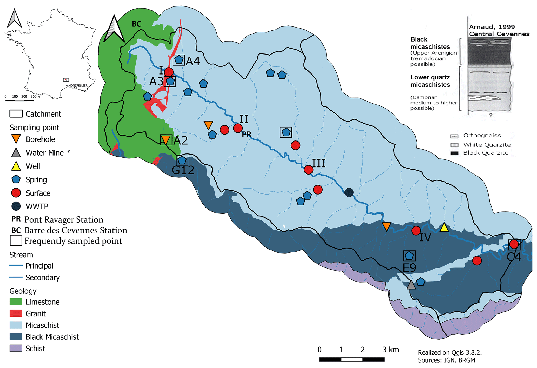
Figure 1 Geology of the watershed studied: Gardon of Sainte-Croix. * A water mine is a horizontal well dug on the mountain slope.

Low-flow values are severe in this watershed, with a discharge rate as low as 100 L/s, namely <1 L/s/km², at the end of the dry season (Fig. 2). Those low-flow levels occur rather late, with a minimum flow often found during September or October. The end of the dry season is determined by heavy autumn thunderstorms typical of the region – this study spans over two years, 2018 and 2019. A large inter-annual variability can be detected in the period between 2017 and 2019. The year 2018 is notable with a relatively high low-water flow, twice as high as in other years. Therefore, it can be assumed that the analysis of the contributions during these periods may shed some light on the differences in processes leading to this inter-annual variability in the flows. The importance of the volumetric discharge rate at the beginning of the monitoring period is linked to the amount of rainfall during winter and spring. However, during the summer period the rainy events have a low impact on the stream's volumetric discharge rate, which shows small and brief peaks following these events. The flow in fact returned to a level lower than that of the flow measured before the event in 1 to 3 d. This implies that the recharge brought by these rains to the subsurface reservoirs is negligible, and hence it is possible to disregard their impact on those reservoirs in our future modelling.

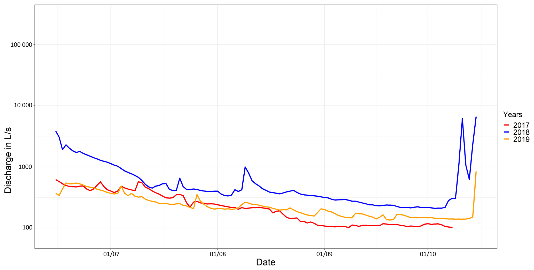
Figure 2 Gardon de Sainte-Croix hydrographs during the low-flow period between 2017 and 2019. The end of the low-flow period is different for each year and depends on the dates of the first important rainfall events. These hydrological data have been measured at the outlet of the catchment (Le Martinet hydrometric station) by the UMR ESPACE 7300 CNRS (Martin et al., 2019).

2.2 Sampling and analysis

To identify the hydrogeochemical end-members, a prospecting campaign was carried out before the low-flow period between April and June 2018. Groundwater samples were collected at 17 sites in the watershed (see Fig. 1). Boreholes were preferred, but only a small number of relevant boreholes exist in the area, so most groundwater samples were collected from springs. The prospecting campaign was completed with existing data from the French National Groundwater Data Access Portal (Lagarde, 2011) to increase the number of observation points and consolidate the characterisation of the geochemical end-members. Physical and chemical parameters (temperature, redox potential, hydrogen potential and alkalinity) were measured in situ at sampling sites. These measurements were carried out using a Hach SL 1000 multimeter. Temperature and electrical conductivity were measured with a CDC 401 probe, pH with a PHC 201 probe and redox potential with an MTC 101 probe. Alkalinity was also measured with a Hach multimeter using the reactive chemkey 8 636 200 for schist and granitic groundwater and chemkey 8 636 100 for limestone groundwater. Samples for the analysis of major ions were collected in closed polyethylene tubes suitable for analyses on the IC (one for the cation and one for the anion). Water was filtered through a 0.45 µm cellulose acetate membrane filter. Tubes for the cation analysis were acidified to pH 2 with a drop of nitric acid titrated to 0.5 N and stored in a cold place until analysis was done within 24 h. A spare bottle of sample was collected to allow double analyses if needed. The analysis was performed by ion chromatography (930 Compact ICFlex, Methrom). Major elements were carried out at the Laboratory of Environmental Isotope Geochemistry, University of Nîmes, EA 7352 CHROME. The mobile phase was prepared in 1 L of deionized water (18.2 MΩ cm at 25 ^∘C) with 50 mL of Na₂CO₃/NaHCO₃ at 64 mM/20 mM for the anions and 25 mL of 2.6-Pyridinedicarboxylic acid at 0.02 M and 2 mL of HNO₃ 3N for the cations. The chromatographs obtained were calibrated according to a series of standards ranging from 0.01 to 100 mg/L for the target ions. Two control samples, one with low concentrations close to water found in metamorphic waters (EC of 50 µS/cm) and the other with high concentrations close to water from sedimentary reservoirs (EC of 600 µS/cm), were analysed at the beginning of each series of analysis as well in order to ensure the absence of instrumental contamination or drift. A verification step was carried out on the integration of the chromatographs obtained.

To facilitate the monitoring during the low-flow period, the observation site area was downsized to two representative sites for each geological reservoir identified as potential end-members. These points were selected based on the results of the prospective campaign and the identification of the geochemical end-members (Table 1). Rainwater samples were collected using the same methodology as for groundwater. The water was collected from a rain gauge located in a neighbouring catchment area less than 10 km south of the catchment.

Table 1 Sampling frequency table detailed over both summers. The bold row in the table corresponds to the main groundwater sites, sampled weekly.

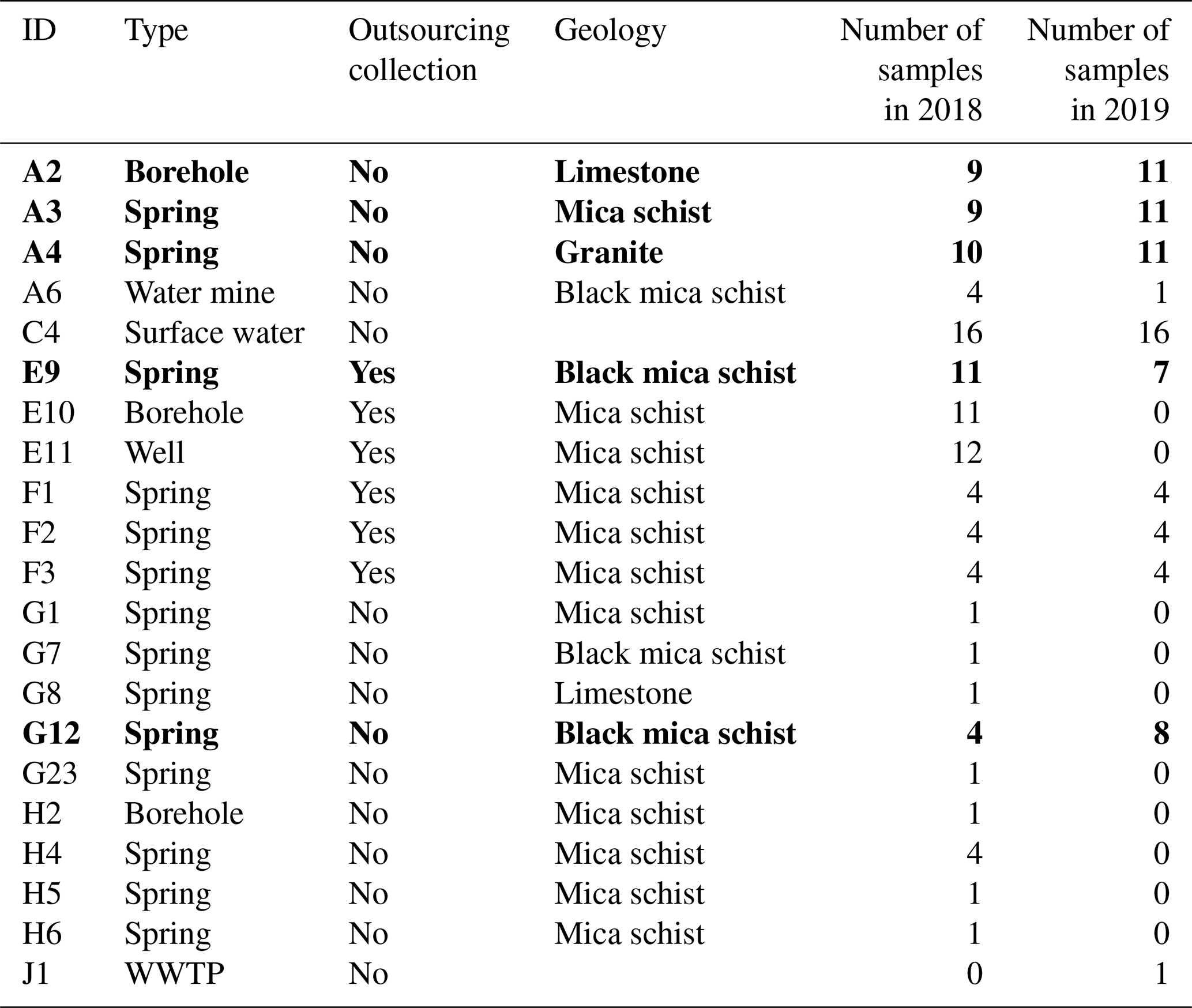
The selection of groundwater sites was made based on logistical reasons because not all sites could be monitored during the low-water period due to their non-perennity or poor accessibility. Springs with groundwater samples showing the influence of several geologies or boreholes located in the alluvial aquifer were also discarded from the monitoring to avoid bias in the characterisation of the end-members as they draw directly on surface water and hence do not represent the geochemical signature of the local geological basement. Two monitoring campaigns were carried out during the summers of 2018 and 2019. Both spanned at least June to October; six springs and borehole sites and one surface water point located at the basin outlet were sampled every week. The 2018 campaign focused on the characterisation of the groundwater contribution during the drying-up period of the river with a high frequency, weekly sampling for surface water and bi-monthly for groundwater. The 2019 monitoring period was complemented to include a spatial analysis where the stream was sampled in four sections (denoted as I, II, III and IV in Fig. 1), and the campaigns including a larger panel of groundwater sampling sites (eight spring or borehole sites) were carried out every month and with sampling continuing until December. The frequency of sampling for this campaign was done every month, both for groundwater and surface water.

Water from the wastewater treatment plant (WWTP) of the main village (Sainte-Croix-Vallée-Française, 350 inhabitants) was also collected for analysis (Fig. 1). An additional campaign was carried out in 2019 to analyse the spatial contribution of tributaries to the main watercourse throughout its route. Gauging and sampling were performed at five sites distributed along the main river and also on six tributaries (three on each side of the river) using the same sampling and laboratory analysis method presented above. The discharge measurements were carried out by the salt dilution method on the tributaries and by exploring the velocity field using a current meter for the main watercourse. The operation aimed to analyse the contribution of the reservoirs with a spatial approach. However, only one tributary on the northern slope could be analysed, as the other two were dry.

2.3 Identification of end-members and selection of representative springs for low-flow surveys

2.3.1 Using groundwater analyses to characterise the end-members

The main assumption behind the geochemical approach is that the stream is a discrete mixture of the different groundwater sources in the watershed. The sample analyses were categorised according to the reservoir geological nature and independent statistical analysis based on different graphical representations. Two diagrams for graphical representation are used: the Piper diagram, which presents the relative concentration of major elements, and the bivariate solute–solute plots that show absolute value results. End-members were defined by investigating the results from these two graphs, seeking to differentiate groundwaters according to the geology of their reservoirs. To validate the identified hydrogeochemical end-members, a principal component analysis (Christophersen, 1992; Long and Valder, 2011) was applied. This PCA was done in R using the FactoMineR package. A definition of end-members by classification was also carried out. This was done by cluster analysis using k-means, a classification method used in other studies (Fabbrocino et al., 2019; Monjerezi et al., 2011; Moya et al., 2015) to define end-members in a more complex system. The k-means analysis was done in R with stats packages. Mean analyses were based on major ion concentrations normalised to the total dissolved solids to avoid dilution. The number of end-members was defined by the average silhouette method defined by Rousseeuw (1987).

2.3.2 Validation of the end-member geochemical signature with a rock-leaching experiment

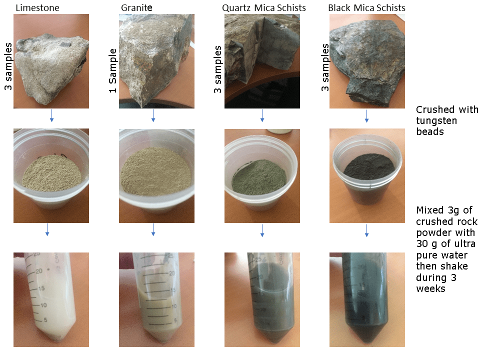
To confirm the validity of the defined hydrogeochemical end-members, a rock-leaching approach was implemented. It aimed to strengthen the validity of the previously defined end-members by using an inverse approach. Rock samples representative of these formations were collected, and the rock-leaching interaction experiment was carried out in the laboratory to ascertain the geochemical signature of the formation representing the geology (see Fig. 3). This approach defined pristine groundwater and allowed us to eliminate end-members showing mixed signatures between formations.

The leaching protocol was based on the widely used Afnor X31-210 standard and other articles (Chae et al., 2006; Gong et al., 2011; Grathwohl and Susset, 2009; Yu et al., 2015). For this purpose, three rock samples if possible were collected in each of the identified geological units at different locations. The rock samples were extracted from the bedrock and all had to be larger than 10 cm-sized blocks. Each sample was then stored individually until analysis. A portion of each sample was set aside for rock sample collection, whilst the rest was crushed with tungsten beads and then sieved through a 4 mm mesh. Rock powder was mixed with ultrapure water (18.2 MΩ) in a 50 mL bottle, with a ratio of $\mathrm{1}/\mathrm{10}$ (3 g rock water to 30 g water). The leaching time was calculated through an experiment to obtain the rock water equilibrium. This test was performed only on a schist sample where a single sample was analysed at several different time steps (1 h, 6 h, 12 h, 24 h, 1 d, 3 d, 1 week, 2 weeks, 3 weeks and 4 weeks), and the stabilisation of the major element point was obtained after 3 weeks. This bottle was then placed in a shaker for 3 weeks at 15 revolutions per minute. The result of this leachate was then analysed on the ionic chromatography machine. Triplicates were made for each sample to improve repeatability and the accuracy of results. Four lithologies were sampled, limestones, granites, black mica schists and quartz mica schists. For each of these formations, three samples were taken from different catchment areas, except for granites, where their limited spatial coverage did not allow multiple sampling sites.

Figure 3 Rock-leaching experiment.

2.4 Mixing analysis

2.4.1 Choice of tracers for mixing analysis

Following the characterisation of the end-members, mixing models were implemented to estimate the contribution of each end-member to the streamflow. This model relies on a sound choice of tracers to calculate the part of mixing. Usually, two to six tracers are considered depending on the number of considered end-members. They often include Ca²⁺, K⁺, Mg²⁺, Na⁺, Cl⁻, ${\mathrm{SO}}_{\mathrm{4}}^{\mathrm{2}-}$, ${\mathrm{HCO}}_{\mathrm{3}}^{\mathrm{2}-}$ and stable isotopes of water as well as physicochemical parameters such as electrical conductivity and alkalinity (Barthold et al., 2011; Bresciani et al., 2018; Burns et al., 2001). In contrast to most research papers, the usual conservative tracers are not considered in this study (the stable isotopes of water, bromides and chlorides), as conservative tracers are not affected by interactions with rocks and hence cannot be used to differentiate the water according to its geological reservoirs (Appelo and Postma, 2005). One of the study objectives was to test a simple method based on common and cheap tracers. Thus major elements are preferred to other more sophisticated tracers such as the strontium isotope ratio, for instance, used in other studies (Rose and Fullagar, 2005). The methodology to define the number of required tracers and the parameterisation for the use of the mixing model were based on a methodology developed by Barthold et al. (2011). This method first investigates correlations between the different tracers in order to eliminate redundant tracers and to retain a number of tracers equal to the number of end-members plus one. Tracers showing little variability or little correlation with the different end-members are also disregarded for this purpose.

2.4.2 End-member mixture model

EMMA was chosen to assess the contribution of the different geochemical end-members identified. Our approach used EMMA coupled with the generalised likelihood uncertainty estimate (GLUE), called G-EMMA and developed by Delsman et al. (2013). This GLUE method, developed by Beven and Binley (1992), manages uncertainties by accepting variations in sets of input parameters. A full range of plausible results can be explored with model executions within a user-defined range by varying the input parameters. The G-EMMA method considers both the uncertainties in the conceptualisation of the model (validity of the choice of end-members) and the measurement uncertainties related to the analytical errors. The variability accorded to the tracers chosen for the surface water is defined by the uncertainty associated with the devices used in the measurement (5 %). A temporal variation treats uncertainties associated with the choice of geochemical poles. Measurement uncertainties are defined by the variation in the measurements of the control samples. Considering this variability makes the geochemical end-member approach more robust by providing results over the full range of plausible results.

In terms of the model configuration, the number of iterations chosen was set at 10⁸. To solve mixtures, all defined end-members and all tracers must systematically be used. The option of “randomsolutes” was activated. This allows the random variation of the order in which the tracers are used in the modelling calculation.

To investigate the impact of the definition of geochemical end-members and its variability, four different methods were envisaged and compared. These methods are sorted in descending order according to their expected robustness and accuracy. The objective was to evaluate the loss incurred in the quality of results between these methods, which demand very distinct degrees of treatment.

• The first approach, the hereafter so-called “time window”. Each end-member is defined by its concentration in elements observed at a specific time in the groundwater and used to calculate the part of the mixture in the stream at the closest time measure of observation recorded in the watercourse (preferably before or, if suitable, just after the measure). The advantage of this method is to consider the seasonal variability of the solute concentration of groundwater.

• The second method, the hereafter so-called “seasonal mean”, considered the mean seasonal value of the groundwaters selected as representative of the reservoir. Therefore, all mixtures are resolved using the average of the groundwater sites previously defined as representative of the formation. The variability given to these end-members is defined by the observed seasonal variability of the end-member.

• The third method, the hereafter so-called “geological mean”, is based on an end-member signature defined by the average of the geochemical signatures of all groundwater collected in the same geological formation for each reservoir without assessment of their representativeness. To give the same importance to each groundwater site, when some were sampled frequently whilst others were sampled just once, the average of the groundwater geochemical signature is calculated at each site before averaging the full results. The variability defines the variability given to these end-members observed in each of the formations.

• The last method, the so-called “leaching method”, uses the results of the leachate experiment and considers these results to be representative of different end-members. End-members are simply calculated by averaging the three leachates carried out for each formation. Due to the relatively small number of samples, the variability of these end-members is defined by the variability of the results added to the ion chromatography analysis results (5 %).

3 Results

3.1 Identification of the end-members

3.1.1 Identification of the end-members by groundwater analysis

In the Piper diagram, three end-members are identified visually (see Fig. 4). The first one (visible in green) is marked by a magnesium and calcium signature for cations and by bicarbonate for anions. This end-member is composed exclusively of water from sedimentary rock reservoirs, mainly limestones and dolomites, and hence is consistent with the composition of limestone groundwater found in the literature (Clark and Fritz, 1997). This end-member is also identifiable in the bivariate solute–solute diagram, where we can see that these waters have conductivity values much higher than other end-members, ranging between 400 and 450 µS/cm, while most of the others are below 100 µS/cm (see Fig. 5). This high conductivity is related to high concentrations of three elements, calcium, magnesium and bicarbonate (3, 2, and 5 mEq/L), while concentrations of other elements remain relatively low.

A predominance of sulfate for anions marks the second end-member (visible in navy). The signature for cations is relatively undifferentiated but tends towards a slightly more magnesian facies. This leads to groundwater marked by a predominance of sulfates ions located in water hosted in the black mica schist formation. However, all springs sampled in this formation did not systematically show an excess of sulfate. In fact, sulfate contents varied from 0.3 to 1 mEq/L. Sulfate remained relatively low for all other end-members. According to previous studies, this sulfated signature could result from schist alteration (Mayer et al., 2010).

Groundwaters from the third pole come from the quartz mica schist reservoir (visible in light blue). The end-member shows a large dispersion with an undifferentiated signature. These waters are characterised by a very low conductivity (less than 60 µS/cm) and a very low concentration in all elements, which strongly differentiates them from other analysed end-members (Fig. 5). Therefore, this end-member can be considered to be undifferentiated; i.e. no element is present in greater proportion than the others. The observed dispersion of the signature in the Piper diagram can be explained by the very low concentrations of elements, leading to a large variation of the geochemical facies due to only small variations of individual element concentrations.

Also presented in Figs. 4 and 5, a unique groundwater sample collected in the granite shows surprisingly high bicarbonate, calcium and magnesium content (2, 1 and 1 mEq/L) and also, to a lesser extent, the presence of sulfates. These concentrations place this sample on the mixing line between two previously defined end-members, the limestone and the black mica schist end-members. The influence of the limestone end-members seems coherent because of the topography and stratigraphic position of the granitic layer crossing the limestone plateau. Moreover, drillings in the area show that the black mica schist layer is present just below the limestone plateau. It is, therefore, possible that springs collected in the granite sections are, in fact, water that percolated through the limestones and then the black mica schists. For these different reasons and the very small extension of the granitic part in the watershed, this reservoir was not considered an end-member.

A seasonal evolution in ion concentrations is clear in both the waters of the black mica schists and the limestones (see Fig. 5). During the drought period, ions concentrations increase, particularly visible for Ca²⁺, Mg²⁺, ${\mathrm{HCO}}_{\mathrm{3}}^{\mathrm{2}-}$ and ${\mathrm{SO}}_{\mathrm{4}}^{\mathrm{2}-}$. This increase in concentration is 12 % for the limestone waters and 20 % for the black mica schist waters.

Finally, a sodium facies marks the water from wastewater treatment plants for cations and high concentrations of sulfates and chlorides for anions with a relatively high electric conductivity (350 µS/cm).

Figure 4 Piper diagram of the groundwater sampled.

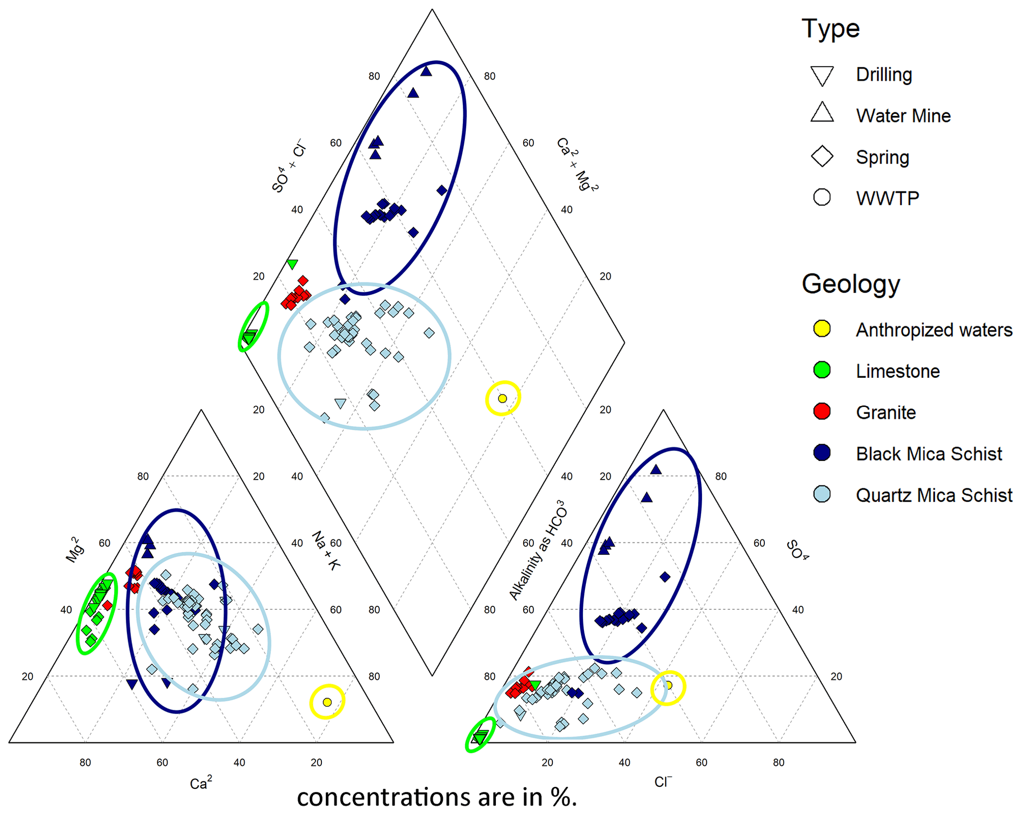
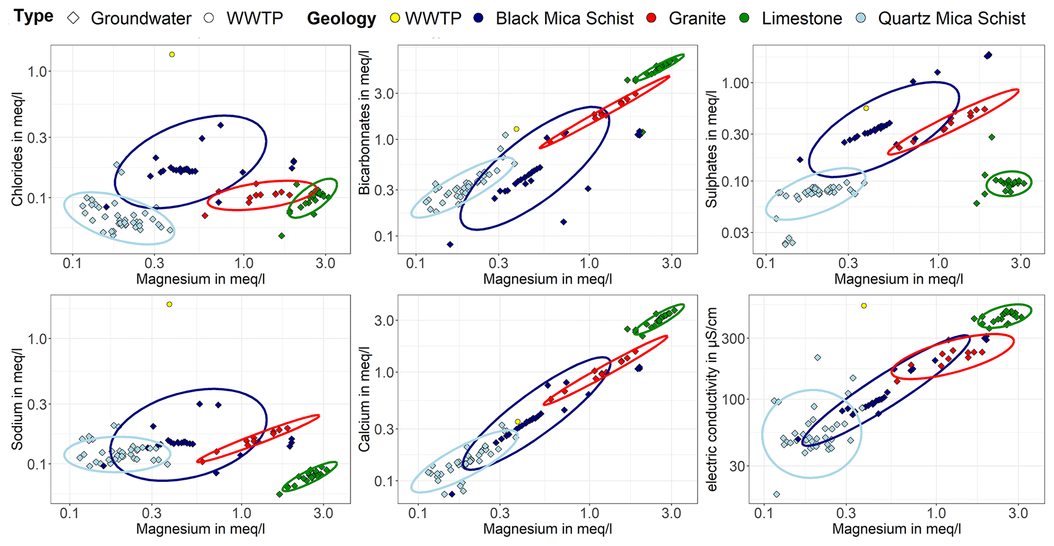
Figure 5 Bivariate solute–solute diagrams of groundwater. The ellipse in the graphs was calculated with stat ellipse (ggplot2 package). The arrows mark the seasonal variation of the different geological reservoirs.

3.1.2 Rock-leaching experiment

The results of the rock-leaching experiments lead to leachate geochemical signatures quite close to the observed signatures from groundwater sample analyses. The differences observed between groundwater and leachate water are of the order of 20 % in conductivity, with lower concentrations on average for leachate water. Four end-members of leaching are visible in the bivariate solute–solute diagrams of groundwater and leachate samples (Fig. 6). These results can be summarised as follows.

• Black mica schist leachates show a high proportion of sulfates and higher magnesium than calcium contents.

• Quartz mica schist leachates are defined by a neutral signature with conductivity lower than 30 µS/cm.

• Limestone leachates are marked by higher Ca²⁺, Mg²⁺ and ${\mathrm{SO}}_{\mathrm{4}}^{\mathrm{2}-}$ content. However, values observed in leachates (1 mEq/L) are 3 times lower than those observed in springs and boreholes (3 mEq/L). This may be inherent to the leaching experiment carried in a closed bottle with a limited quantity of CO₂. The lack of exchange with the atmosphere during the leaching process could indeed limit the concentration of dissolved elements in the leachate (Appelo and Postma, 2005).

• A granite pole marked by the presence of sodium and potassium in very large quantities can be identified here. The obtained leachate geochemical signature differs from that observed for the groundwater collected in this formation (showing both low Na and K contents).

  Large amounts of potassium are observed in the leachates of the crystalline rock samples typical of the weathering of potassium feldspars (Appelo and Postma, 2005; Clark and Fritz, 1997). Since no collected water shows this signature marked in sodium and considering that this layer has a very small spatial footprint, this granitic reservoir is disregarded from the estimations of the contributions to streamflow.

Leachate results raise questions regarding the relatively large amount of potassium in the metamorphic rock samples. These quantities are 3 times higher than those observed in the groundwaters. These differences can be explained by the leaching method (crushing of the rocks to a very fine granulometry), which favours the potassium solution via the alteration of potassium feldspars (Appelo and Postma, 2005; Clark and Fritz, 1997), while K in situ may already have been leached.

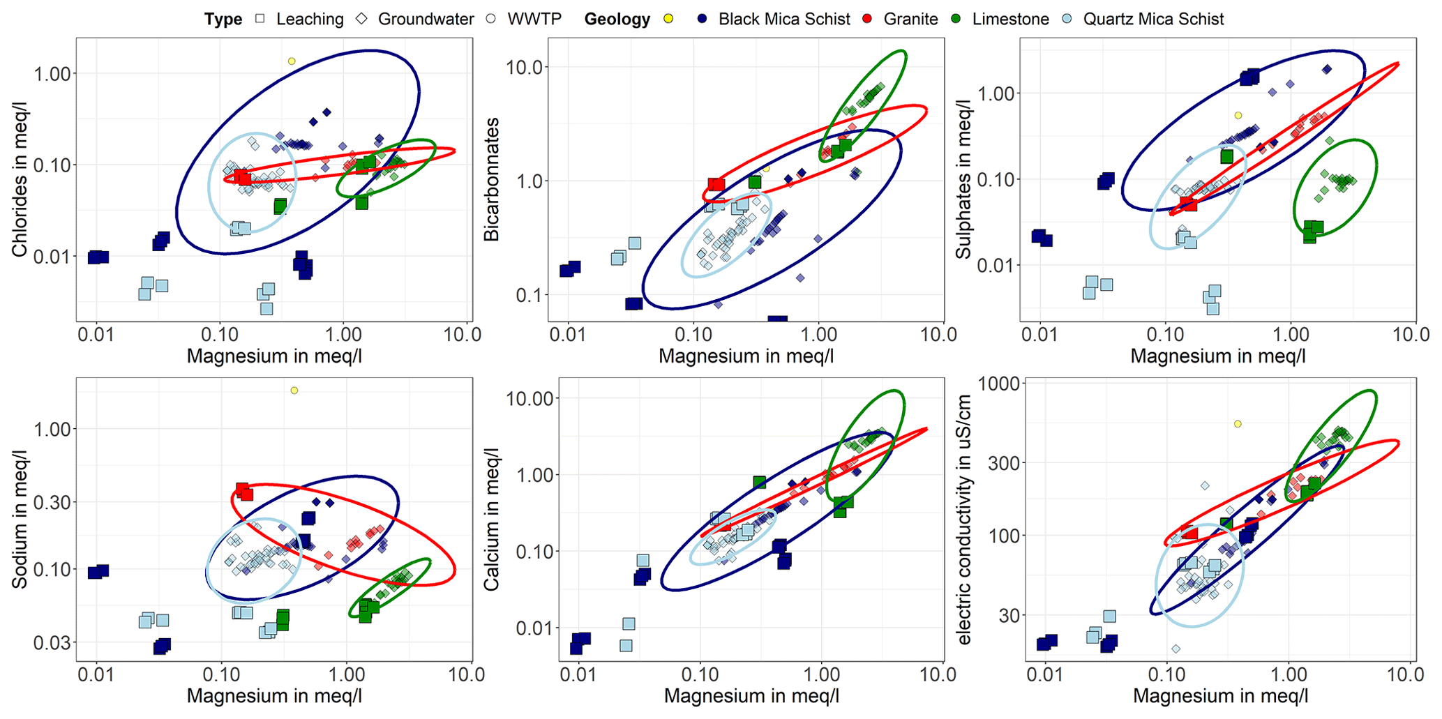
Figure 6 Bivariate solute–solute diagrams of the leachate result with the groundwater sample.

3.1.3 Validation of the end-member by statistical classification

In order to confirm the end-members' characterisation and clustering independence, a statistical approach has been carried out on collected groundwaters. Focussing on the groundwater end-member analyses, the WWTP's water was not included in the statistical analysis. The first step in this method is to define the number of clusters. The inertia curvature of groundwaters shows in both cases that the optimum number of classes is three (Fig. 7). This number of three classes corresponds to the number of identifiable end-members found in the catchment. This number is to be used for upcoming k-means analyses.

Figure 7 Silhouette values to define the optimal number of clusters.

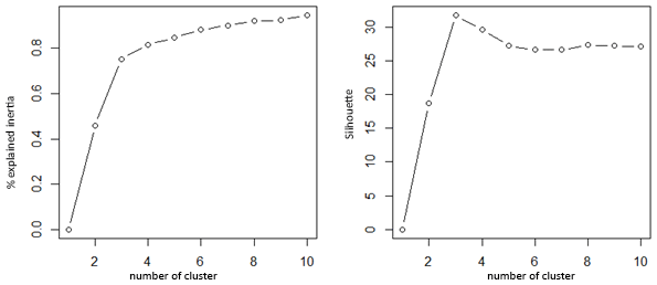
Inertia curves define an optimal value of three classes and give equivalent results to previous analyses on groundwater samples to characterise the end-members. Moreover, the three clusters defined by this method correspond to the three identified end-members and hence to the three main geological reservoirs, namely limestone, quartz mica schists and black mica schists.

Indeed, the first cluster is defined by a low conductivity and a high proportion of bicarbonates in the water, which is consistent with the quartz mica schist reservoir (Table 2).

The second cluster is defined by high sulfate and magnesium proportion and corresponds to the black mica schist reservoir. The third shows a high proportion of calcium, magnesium and bicarbonates in the water and high electrical conductivity, which is consistent with the limestone reservoir.

The locations of the groundwater samples, identified by clusters, are plotted on the geological map showing the good correspondence between the three clusters and the three geological reservoirs (see Fig. 8). Only two outliers are visible. The first corresponds to the point present in the granite formation and previously identified as a mixture of limestone and black mica schist. The second corresponds to the black mica schist spring identified by the classification as being from the quartz mica schist pole. Conversely, the K-means method attributes this point to the sedimentary rock clusters in coherence with the mixing hypothesis of groundwater issued from limestone and black mica schists.

Table 2 Mean proportion in percentage of the major elements in the cluster results.

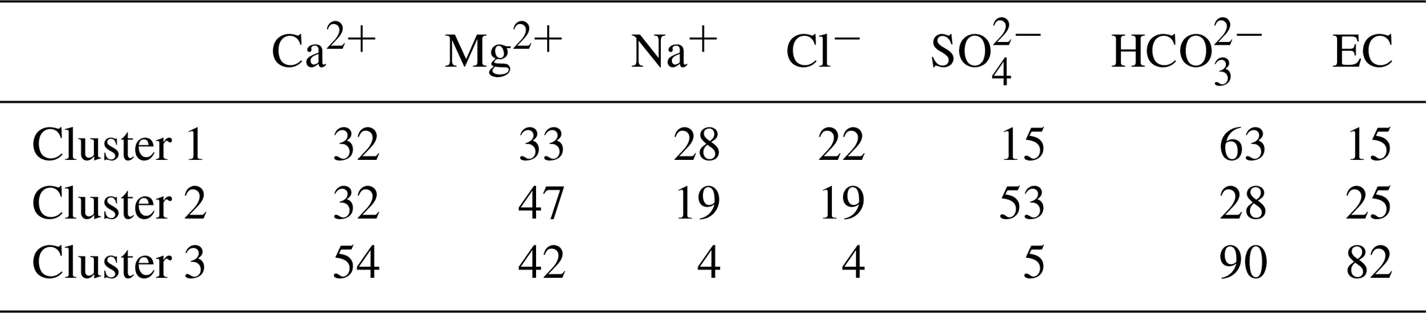
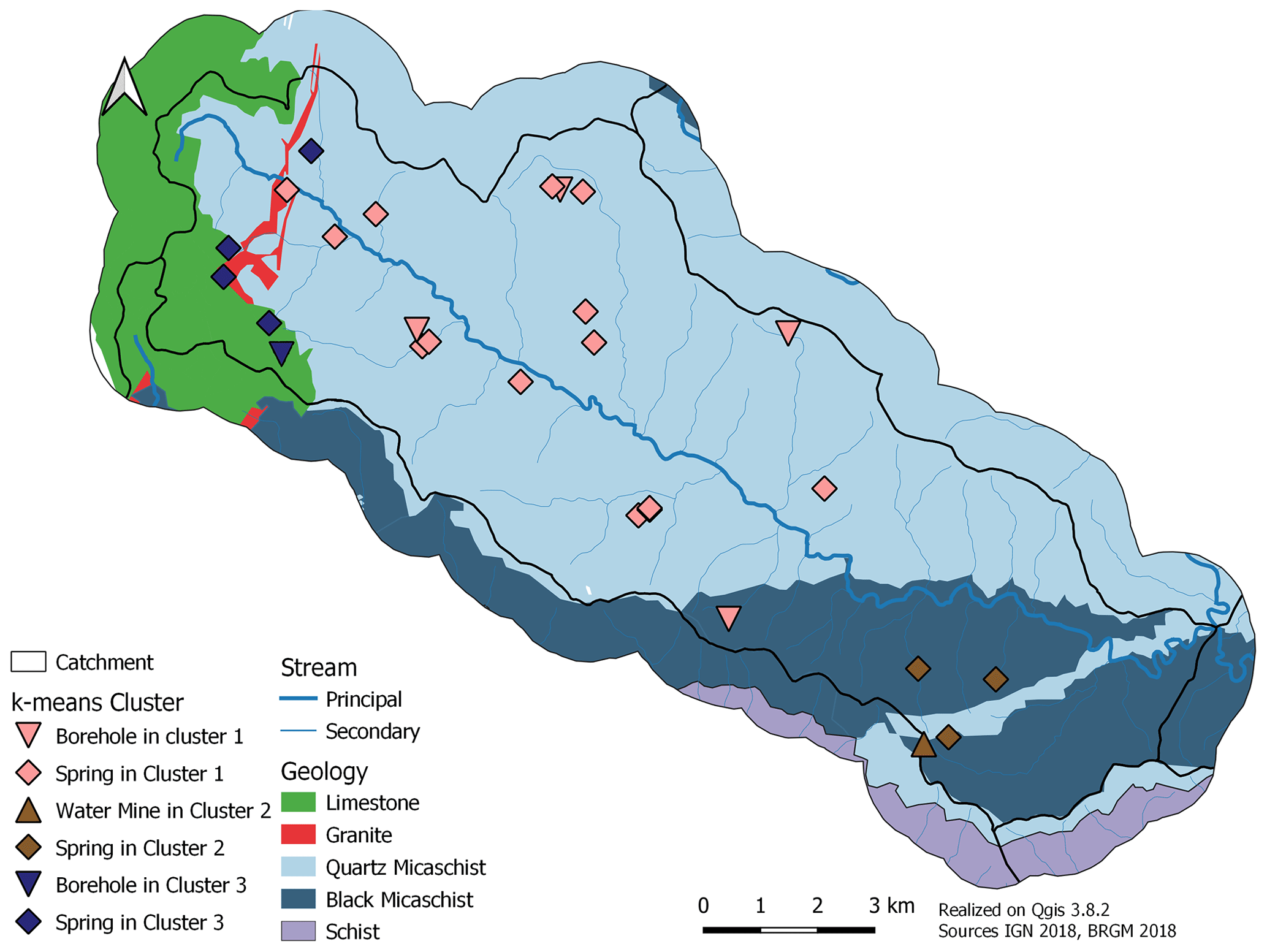
Figure 8 Cluster localisation obtained with the k-means method.

3.2 Mixing results

3.2.1 Choice of tracers

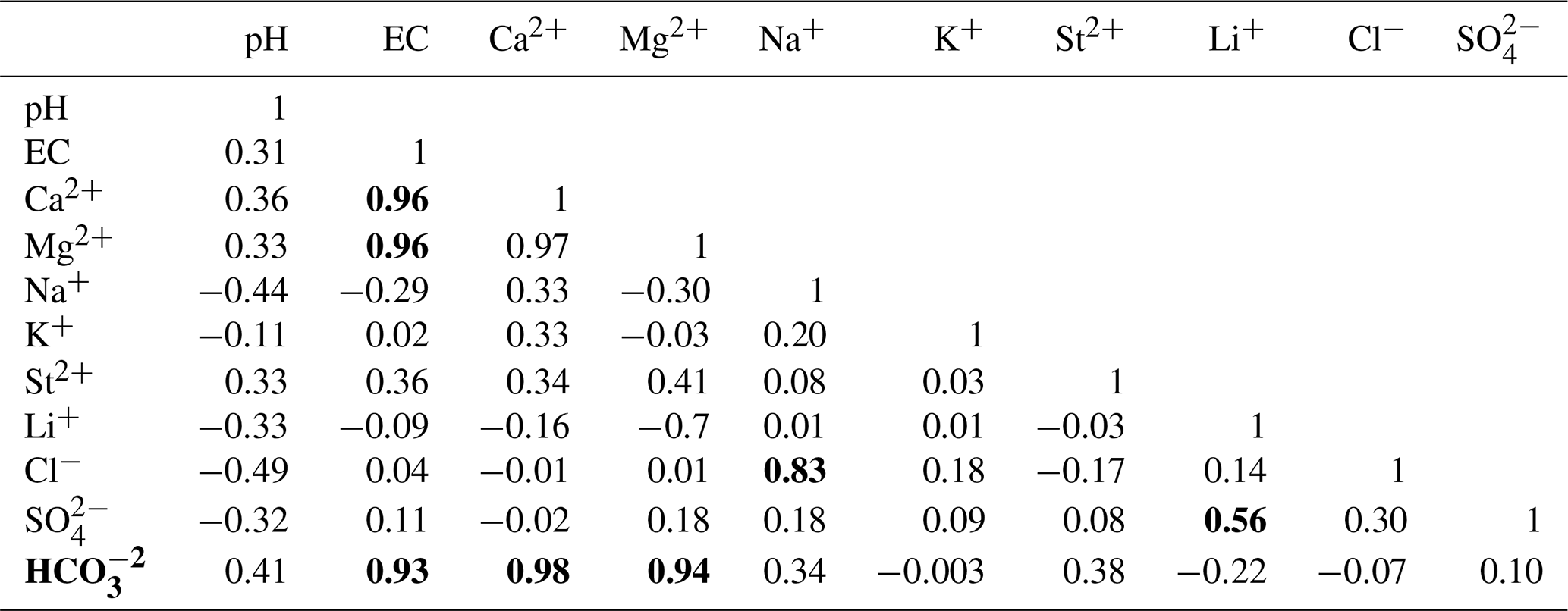
Regarding the choice of tracers used in the mixing model, previous studies, such as Barthold et al. (2011) and Christophersen (1992), recommend disregarding those with overly strong inter-correlation or overly weak variances. The principal component analysis (Fig. 9) shows the strong correlation between the limestone end-members (in green) with the Ca²⁺, Mg²⁺, HCO₃²− and Sr²⁺ tracers. Black mica schist (in navy blue) is significantly connected to ${\mathrm{SO}}_{\mathrm{4}}^{\mathrm{2}-}$ and to a lesser extent to Cl⁻ and F⁻. The pole of quartz mica schist (in cyan) shows a very low variance with both axes. However, it shows a slight inverse correlation with the axis 2, the variance of which is explained by ${\mathrm{SO}}_{\mathrm{4}}^{\mathrm{2}-}$.

Figure 9 Principal component analysis.

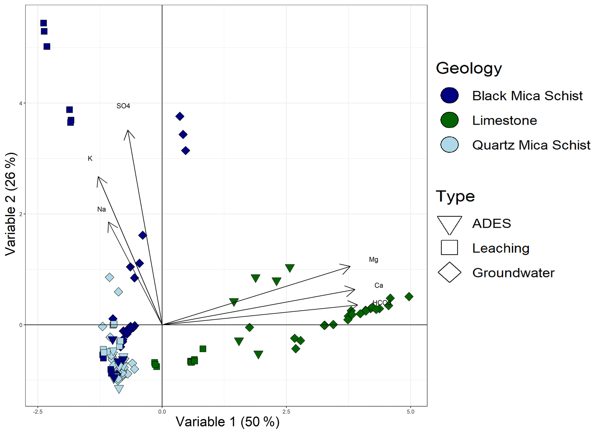
Based on those observations, the selected tracers are ${\mathrm{HCO}}_{\mathrm{3}}^{\mathrm{2}-}$, ${\mathrm{SO}}_{\mathrm{4}}^{\mathrm{2}-}$, Mg²⁺ and Na⁺. ${\mathrm{HCO}}_{\mathrm{3}}^{\mathrm{2}-}$ was selected for its correlation with the limestone end-members and ${\mathrm{SO}}_{\mathrm{4}}^{\mathrm{2}-}$ for its correlation with the black mica schist end-member. Sodium was also selected due to its connection with the wastewater pole. Minor ions have been disregarded because they are often below the detection limits, particularly for fluorides in limestone water. Due to the low concentration of total dissolved solids in all measured dissolved ionic elements of groundwater from the quartz mica schist reservoir, no tracers were specifically identified for this reservoir. This reservoir acts as a dilution end-member for all tracers. Low mineralisation in all tracers is the marker of this end-member. To improve the efficiency of the model and to conform with and follow the methodology developed in Barthold et al. (2011), the choice was made to add one additional tracer to the tracers chosen by the end-members. Due to their strong explanation of variance, calcium and magnesium were selected, but with the high correlation between these elements (Table 3), only magnesium is selected to limit the weight of the calcareous water contribution to the mixtures. Magnesium is preferred to calcium because it is slightly correlated with the pole of black mica schists, making it more relevant and different to bicarbonates (Fig. 9). These selected tracers have the particularity of being reactive in groundwater reservoirs, allowing them to be marked by the passage in this reservoir, but it can be considered conservative in the watercourse. In the stream, water–rock interactions are reduced, and equilibrium is rapidly obtained with the atmosphere. The measurement of dissolved oxygen in the springs confirms this by revealing identical oxygen concentrations to those found in the streams.

Table 3 Correlation matrix. The bold values show the correlation greater than 0.5.

In this analysis, it is evident that it is impossible to differentiate waters of quartz mica schists and rainwater. Rainwater collected in the area has an electrical conductivity of 14 µS/cm, only slightly lower than that of the mica schist water, which has an average electrical conductivity of 44 µS/cm². Moreover, rainwater shows an undifferentiated signature, similar to the water from the quartz mica schist reservoir. Hence, this model must be used exclusively in low-flow conditions so that the proportions of water identified as issued from quartz mica schists are not confused with the portion issued from rainwater.

3.2.2 Result of the mixing analysis of the time window method

The results obtained using the G-EMMA with the “time window” method are shown in Fig. 10. To start with, it is noticeable that both summer periods, 2018 and 2019, differ strongly in terms of hydrology. The Gardon de Sainte-Croix discharge varied from 600 to 200 L/s in 2018 and from 300 to 150 L/s in 2019. These differences in flow rates can be explained by higher cumulative precipitation in spring 2018 (700 mm) than spring 2019 (375 mm). This difference in the amount of precipitation is interesting as it allows for comparisons of the behaviour of this river system both during low flow and the slightly more severe drought period. Nevertheless, the mixing model gives overall relatively similar results for both summers. A relatively limited contribution from sedimentary rock reservoirs (under 10 %) is observed, while the largest part came from schist rocks (90 %). The quartz mica schists and black mica schists contribute roughly the same proportion at the beginning of the summer (see Fig. 10), and then a decrease in the contribution of quartz mica schists and a relative increase in the contribution of black mica schists is evident towards the end of the dry season. WWTP effluents show an extremely low contribution of 1 % to 2 %. A more important contribution of WWTP can be observed from mid-July to the end of August, consistent with the decrease in natural streams and the increase in WWTP effluent due to the increase in population during summer but remaining nevertheless below 4 %.

The distribution of the calculated contributions allowed by the model is very low for the results on water contributions from the limestone end-member and WWTPs, remaining below 1 % of the contribution. They are greater for schist waters, ranging from 10 % to 25 %. The relative similarity in mineralisation between the two end-members (quartz mica schist and black mica schists) and their dispersion leads to a wider range of possible results.

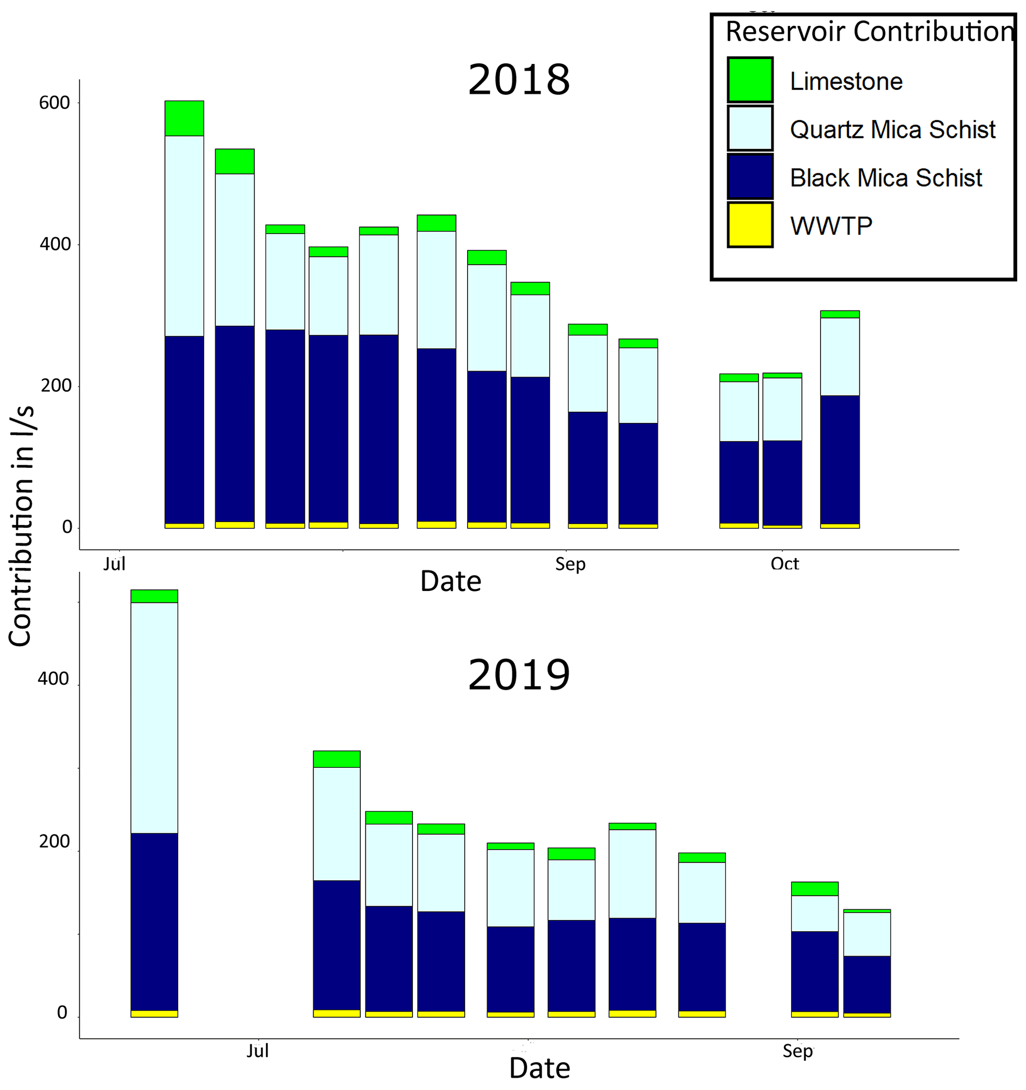
Figure 10 Evolution of the contribution of the various reservoirs during the summers of 2018 and 2019. The difference in the number of samples between 2018 and 2019 is due to the differences in sampling frequency between the two years, weekly and fortnightly for 2018 and for 2019 respectively. The uncertainty associated with these proportions is less than 15 % for WWTP and limestone waters and less than 35 % for quartz and black mica schist waters.

At the beginning of the monitoring period in 2018, the quartz mica schists brought 290 L/s and dropped to 75 L/s in low flow, while the black mica schist reservoir contribution varied only from 270 to 130 L/s. In 2019, the quartz mica schist contribution brought 120 L/s initially and dropped to 30 L/s at the end of the low-flow period, whilst black mica schist flow only dropped from 160 to 90 L/s.

Expressed in percentage of the flow rate, in 2018, the contribution to the flow rate is about 45 % for the black mica schist reservoir and 50 % for quartz mica schists. At the end of the summer, the contribution of the quartz mica schist reservoir drops slightly to 30 %, while the black mica schist reservoir provides 65 % of the flow. For the year 2019, the contribution is already unequal at the beginning of the season between the two formations, with nearly 55 % ensured by the black mica schists and 45 % by the quartz mica schists. The relative contribution of the black mica schist reservoir increases significatively during low-flow conditions, where it reaches 75 % of the total flow. The limestone reservoir shows a relatively low contribution whilst remaining relatively constant with a value between 5 % and 10 % throughout both summers. Hence, at the beginning of the summer (June 2019), most of the water flow comes from quartz mica schists, while the contribution of the black mica schists became preponderant during the low-flow period. Surprisingly, the contribution of the black mica schist reservoir is very high for the small surface area of this formation outcrop, approximately 20 % of the surface area.

The decreasing flow rate is very different between both schist reservoirs. It shows relatively equivalent flows at the beginning of the season, which decreased during the dry season, with a reduction of the flow by a factor of 4 for the quartz mica schists and only by a factor of 2 for the black mica schists.

The drying curve of these two reservoirs is consequently very different, reflecting two very different behaviours with a much steeper slope and therefore demonstrating a much lower low-water production capacity for the quartz mica schists during the low-flow period. The specific flow rates calculated with respect to the outcropping surfaces of each geology are less than 1 L/s/km² for quartz mica schists and more than 2 L/s/km² for black mica schists. All of this highlights the importance of the black mica schist reservoir in the maintenance of the discharge during low-flow period levels. The contribution of this reservoir became even more essential in times of extremely low flows.

3.2.3 Uncertainty of mixing analysis

To compare the results obtained with the different approaches considered for end-member signature characterisation, the outputs of the four models (time window, seasonal mean, geological mean and leaching experiment) were plotted together in Fig. 11. All four approaches gave similar results and trends to those observed with the time window method. Dispersion in the contributions remained high, reaching a variation of 25 % between the two quantiles and nearly 50 % between the limit of the models: time window and seasonal mean present low dispersion in the range of possible contributions. However, general trends seen in contribution graphs remain identifiable and consistent from one model to another, with an increase in the contribution of black mica schists and a decrease in the contribution of quartz mica schists during summers. The first autumn rains can explain the steep increase in the contribution of quartz mica schists and the decrease in black mica schists' contributions at the end of the season. The autumn rains reverse the contribution of these two reservoirs as they recharge the quartz mica schist reservoirs, which are much larger in surface area than those of the black mica schists and directly dilute the river water, acting as a contribution of the quartz mica schist reservoir diluting the surface water.

Figure 11 Mixing model result uncertainties for different contributions. The green colour represents the contribution of the limestones, the cyan represents the contribution of the quartz mica schists, the dark blue represents the contribution of the black mica schists and the yellow represents the contribution of the WWTP waters. For each variable the central line is the median value of the model, the outer limits are the limits of the model (respectively 5 % and 95 %) and the limit of the darker colours corresponds to the quantile of the model. The contributions are expressed in an index ranging between 0 and 1, where 1 corresponds to the sum of the contribution.

Differences are nevertheless visible between the four outputs. The selection graph by geology, which uses average values of all water collected in the same formation, shows the greater variability for the contribution of the quartz mica schist reservoir. This variability can be explained by a larger dispersion in water signatures encompassing all groundwater analyses over the observed period, thus integrating seasonal variations and leading to the definition of less constrained end-members. This gives the model greater freedom in solving mixtures.

The “leaching method” also shows less constrained outputs. These are mainly visible in the contribution of the limestone pole, of which the contribution is more important than for the other three model outputs. This relates to the fact that the limestone leachate end-member is artificially less concentrated than other approaches, leading to an overestimation of its contribution. There is also a difference between the “time window” method and the “seasonal mean” method, while the signal appears smoothed. This difference can be explained by account being taken or not of the seasonal drift (see Fig. 11). Regarding the “seasonal average” output, the results show a lower contribution of the waters with the highest low-flow electrical conductivity (limestone) and a higher contribution of the waters with the lowest electrical conductivity (quartz mica schist).

3.3 Spatial analysis of modelling results

The investigation of the spatial distribution of the different reservoir contributions was carried out. This spatial approach consisted of collecting samples and measuring the flow rate along the river length along with the main tributaries on the same day. This campaign was carried out during the 2019 low-water period (10 October). At that time, the measured flow rate was 142 L/s, while this year's lowest flow rate was 135 L/s. The measurement was performed on the three biggest tributaries on the right and left banks. Only one of the targeted tributaries was surveyed on the left bank, as all other streams had dried out.

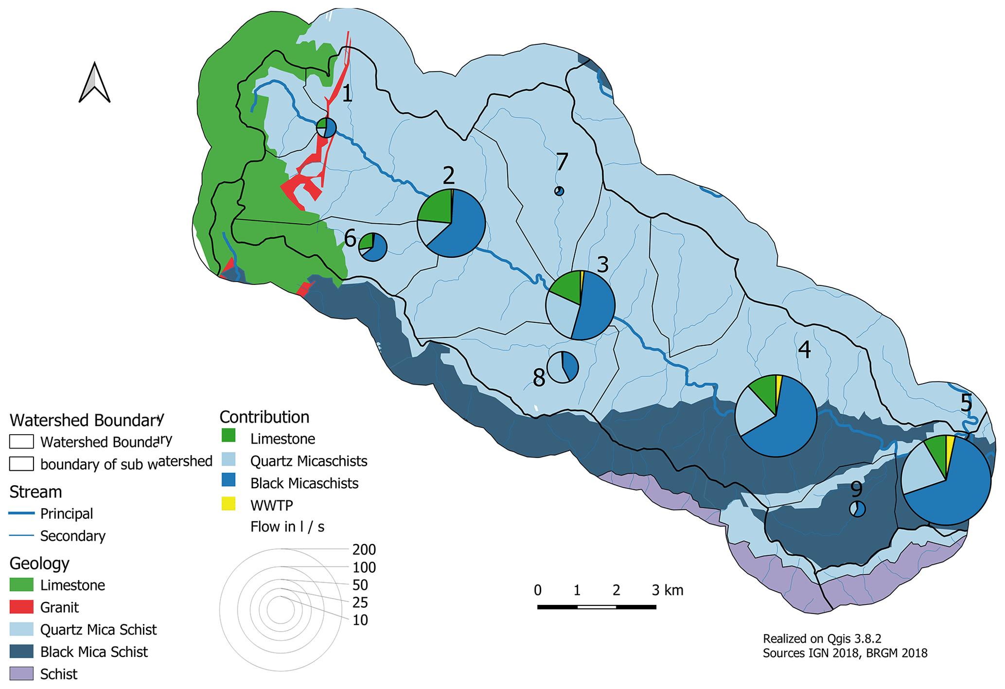
Figure 12 Map of the contributions of the different aquifers in the Gardon de Sainte-Croix basin on 11 October 2019.

The results underline the black mica schists' predominant contribution to low flow throughout the watershed (see Fig. 12). The results also show an uneven spatial distribution of the specific flow rate. The mainstream specific discharge varies widely from the headwater to the outlet, with more than 2 L/s/km² at the most upstream section (stations 1, 6 or 8), decreasing to approximately 1 L/s/km² at the outlet (station 5). With regards to the tributaries, the differences are even greater, with specific flows of less than 0.1 L/s/km² on the northern slope (left bank, station 7) and reaching nearly 2 L/s/km² on the southern slope (right banks 6, 7, and 9). The contribution of the upper limestone reservoir remains nevertheless a minor contribution (<20 %, at stations 1 or 6) and cannot explain the observed upstream high-flow rates. It is noticeable that the upstream flow already relies heavily on the black mica schist and quartz mica schist reservoirs. The high upstream and southern slope-specific flow rates may be explained by the presence of a black mica schist stratum, identified as the main source of water during low-water levels, located below the upper limestone plateau and extending on the southern slope (Arnaud et al., 2004). In terms of contribution levels, the black mica schist reservoir remains the main contributor throughout the basin. The quartz mica schist reservoir contributes only as a secondary source, of the order of 25 % of the low-flow rate, except on a tributary of the southern slope located downstream of the watershed. The WWTP contribution is insignificant in small tributaries and increases slightly downsteam along the mainstream with increasing urbanisation.

4 Discussion

4.1 Are the identification of mixing poles and the significance of geochemical end-members correct?

Mixture models are powerful tools that can deal with many scenarios and thus provide a wide range of possible solutions (Soulsby et al., 2003; Uhlenbrook and Hoeg, 2003). They deliver valuable information if the decisive parameters, such as uncertainties and end-members, are properly considered. The main challenge in studies using this tool concerns the availability for the end-member identification and the definition of their signatures. Regarding the first point, in this study, where the identified end-members match the geological reservoirs, it must first be demonstrated that the geochemical signature of water in the different geological reservoirs differs significantly according to the geology. The approach chosen in this article to address these issues is multi-faceted. It is based on a geological analysis of the groundwater collected in the basin consolidated by two complementary approaches. The first one is based on rock leaching, which confirms that the defined end-member signatures are sound and proves that the springs collected in the formations reflect well the formation's geochemical signature. The second is based on a supervised classification that allows the validation of the idea that the end-members are distinguishable by the geology of their reservoir.

The definition of the correct geochemical signatures of the different poles is complicated by the seasonal variation of the concentration in groundwater. This increase in different ion concentrations (Ca²⁺, Mg²⁺, ${\mathrm{SO}}_{\mathrm{4}}^{\mathrm{2}-}$, and ${\mathrm{HCO}}_{\mathrm{3}}^{\mathrm{2}-}$) during summer observed in groundwater can be explained by a decrease in precipitation leading to both a decrease in the dilution process of groundwater and a possible increase in the residence time of water in the reservoir and thus an increase in concentrations. A standard method, used in most studies, focusing on flood events, recommends using extreme values to characterise the signature of each pole (Ali et al., 2010; Christophersen, 1992; Correa et al., 2019; Genereux, 1998; Iwasaki et al., 2015). However, for the groundwater reservoir with the highest mineralisation, if only the high extreme values are considered to define the signature of the end-member, the amount of water contributed by the less mineralised water of this reservoir, i.e. with a higher dilution and a shorter residence time, would be underestimated in the mixing part of the calculation. This would lead to an underestimation of the contribution of these reservoirs in terms of volumetric flow. Conversely, for the reservoirs with the lowest concentration of dissolved elements, the choice of the most diluted end-member would lead to an overestimation of their contribution to the volumetric flow. Furthermore, the natural variability in the geochemical signature of different water samples taken from the same formation or leachate illustrates some heterogeneity in the geological formation or the weathering conditions and the need to consider a more appropriate value for defining end-members rather than a maximum or minimum.

In response to this issue, we tested four different methods to define the end-member signatures and assess their relevance. As a reminder, the first two are based on the analysis of collected groundwater defined as representative of a specific reservoir, one considering the “seasonal mean” of the groundwater geochemical signature as an end-member and the other taking into account the geochemical signature of the groundwater samples, collected at roughly the same time as the modelled surface water. The third method considers an average signature on all groundwater samples from the geological formation over the entire watershed, the “geological mean” approach and the last one based on the results of the rock-leaching experiments, the leaching approach. It appears that the methods based on rock leachate analyses and the “geological mean” present structural limitations. Regarding the leaching approach, the shortcomings are linked to the limestone leachate experiments, with leachates showing significantly lower mineralisation than was observed for the groundwater for the limestone rock formation due to a close system concerning the gas CO₂ during the leaching experiment, imposed by the experimental conditions. Regarding the “geological mean” method, the over-representation of the data on water collected during the pre-campaign period, between March and May 2018, i.e. in a hydrological situation of low average flow, induces an underestimation of the mineralisation of the end-member and an increase in the standard deviation (caused by a wider range of results). This leads to high variability in the obtained results and their uncertainties.

The other two approaches, the “time window” and “seasonal mean” approaches, give very concordant results. However, slight discrepancies appear in the modelled parts of mixing (see Fig. 11). This is especially visible in the second part of the summer of 2018, when the “time window” method differs from the “seasonal mean” method, showing a minor decrease in the black mica schist reservoir contribution and a minor increase in the quartz mica schist reservoir contribution. This discrepancy may result from the impact of a heavy rainfall episode that fell at the beginning of August in the basin (about 30 mm), inducing a visible dynamic after this event. This result suggests that the average seasonal method would not consider certain variations during the low-water period due to its excessive smoothing of the poles. Therefore, the “time window” method would allow for results with greater temporal precision. Moreover, the absence of considering the seasonal variations of the end-members leads to an overestimation in low flow of the mixing proportions of the reservoirs with a greater seasonal increase than the others. Despite the greater fluctuations for the “time window” method, it gives visibly finer results and allows a good understanding of temporal dynamics.

Based on those observations, it can be recommended to use the time window approach to identify the signature of end-members in a context of significant seasonal variability. The other approaches allow one to assess the trends but are not precise enough to compute the precise part of mixing.

4.2 Discussion of the results

The study of the contribution at the level of the watershed's outlet or, more generally, over the whole watershed shows the importance of black mica schists during low-water periods. At the beginning and at the end of the low-water periods, it can be seen that the majority of the water flow comes from the quartz mica schists. Nevertheless, the contribution of the black mica schist reservoir remains very important considering its small surface area, making up only 20 % of the catchment area. The drying curves of these two reservoirs are very different, reflecting two very different behaviours with a much steeper slope and demonstrating a much lower water production capacity in low-water levels for the quartz mica schists during the low-flow period. The specific flows in low flow calculated with the outcropping surfaces of each geology are less than 1 L/s/km² for the quartz mica schists and more than 2 L/s/km² for the black mica schists. All this underlines the importance of the black mica schist reservoir in supporting the low-water levels, which is even more marked when the flows are lower.

The analysis of the spatial distribution is in agreement with the location of the reservoirs and provides relevant results on the distribution of the productive reservoirs. We can see that the black mica schists are the biggest contributors, and the main resource area of this formation comes from the upstream part of the catchment. This result may appear contradictory due to the absence of outcrops of this formation in this part but can be justified by the presence of this formation under the limestone plateau (Arnaud, 1999). Other factors support this assertion: on the slopes where the black mica schists are inexistent, the flow rates are much lower than on the rest of the basin, and almost all of the tributaries dry up during severe low water. These results allow the clear identification of the main reservoir in the low-water support and could be used to guide streamwater management in this catchment area to preserve the resources of this essential reservoir.

These robust results in the contribution consolidate the conclusions made by other authors, who highlight the importance of groundwater in the hydrology of mountain areas (Gabrielli et al., 2012; Hale et al., 2016; Uchida et al., 2006). Nevertheless, the significant contribution of groundwater from metamorphic rocks in the basin is in contrast to traditional hydrological assumptions that consider such basement rocks in mountainous regions as having limited aquifer potential (Younger, 2007). However, there are significant differences between both schist reservoirs, with overall higher contributions from the black mica and lower contributions from the quartz mica schists. The analysis of the tributary contributions highlights an ever-greater variability linked to the upstream–downstream and southern side–northern side oppositions. These show that the flow is mainly produced during low flow on the southern slope and, more precisely, in its upstream part. The contribution is mainly from the black mica schists in this upstream zone. One another tributary (the Valat des Oules 8 in Fig. 5) has a very high specific flow (1.7 L/s/km²), with contributions coming mainly from the quartz mica schists. This singularity lends credence to another hypothesis in which this difference in low-water runoff generation comes from a difference in weathering in the mica schists. This difference in alteration would give the more weathered rocks a greater storage capacity and higher runoff generation at low water.

This higher runoff generation of the weathered zone has been evidenced in other studies (Floriancic et al., 2018; Mwakalila et al., 2002; Smith and Patton, 1981; Witty et al., 2003). It was shown that these weathered zones (e.g. saprolite or other regoliths) can serve as a larger baseflow maintenance reservoir than the underlying bedrock (Smith and Patton, 1981; Witty et al., 2003). This possible predominance of the weathered zone causes complications in interpreting the influence of bedrock type on baseflow due to the difficulty in separating it from the contribution of the unweathered zone (Mwakalila et al., 2002). It would be relevant to test methods to differentiate these contributions such as the investigation based on the lithium isotopes ((Millot et al., 2010)). Others may be considered: indeed, a more important fracturing of a rock may cause great differences in contributions (Uchida et al., 2006), or the orientation of the schistosity plane of the layers oriented mainly may move towards the north (Arnaud, 1999), which can lead to more important storage of the reservoirs on the southern slope and more rapid drainage of the groundwater from the northern slope.

5 Conclusions

The results presented in this article are convincing. They show that the use of tracers, as basic as major elements, was revealed to be relevant in identifying the contribution of the different geological reservoirs to streamflow during a low-flow period in small catchment areas. The method using groundwater major element analysis of each geological reservoir to characterise the end-members leads to sound results and validation by statistical analysis, and rock leaching analysis provided robustness to the end-member characterisation. Hence, the paper's first objective is validated: to identify and characterise the contributors to the streamflows based on simple major element analysis.

The second objective relates to the quantification of the contributions of each identified end-member. The different approaches used to characterise the geochemical signature of the end-member, i.e. “time window”, “seasonal mean”, “geological mean”, and “leaching”, lead to comparable results. The distinction of a specific geochemical end-member associated with each geological reservoir and the measure of discharge rates allowed us to quantify their contributions to the river flow. The results outline the discrepancy between the outcropping surface area of each geological reservoir and its contribution in terms of flow to the river.

It can be seen for this catchment area that the black mica schist reservoir becomes the predominant contributor during low-flow periods, although it only occupies a relatively small spatial coverage. Moreover, the spatial analysis of flow contributions shows that the main contribution of this formation comes from the upstream part of the catchment, where this formation hardly outcrops. Therefore, we can foresee a relatively large cover reservoir of this formation in this part of the catchment. These results highlight the key role of this reservoir and alert the stakeholders to the need to efficiently manage and preserve these specific water resources, especially under increasing pressure and the effects of climate change.

These encouraging results were probably facilitated because the basin is relatively simple from a geological perspective and shows very little anthropic activity that could significantly impact the river's chemistry and complexify the analysis. It would appear relevant to test this method in more complex catchments and/or those with a higher anthropic impact. The results of this study underline the predominance of a reservoir, with a small spatial extent in the support to low-water periods of the basin as a whole. They highlight the importance of a greater understanding of the functioning of watersheds at low flows to develop a better strategy for the management and preservation of the resource due to future climate trends.