the Creative Commons Attribution 4.0 License.
the Creative Commons Attribution 4.0 License.
 | 06 Dec 2021
Coherence of global hydroclimate classification systems
Kathryn L. McCurley Pisarello
James W. Jawitz
Climate classification systems are useful for investigating future climate scenarios, water availability, and even socioeconomic indicators as they relate to climate dynamics. There are several classification systems that apply water and energy variables to create zone boundaries, although there has yet to be a simultaneous comparison of the structure and function of multiple existing climate classification schemes. Moreover, there are presently no classification frameworks that include evapotranspiration (ET) rates as a governing principle. Here, we developed a new system based on precipitation and potential evapotranspiration rates as well as three systems based on ET rates, which were all compared against four previously established climate classification systems. The within-zone similarity, or coherence, of several long-term hydroclimate variables was evaluated for each system based on the premise that the interpretation and application of a classification framework should correspond to the variables that are most coherent. Additionally, the shape complexity of zone boundaries was assessed for each system, assuming zone boundaries should be drawn efficiently such that shape simplicity and hydroclimate coherence are balanced for meaningful boundary implementation. The most frequently used climate classification system, Köppen–Geiger, generally had high hydroclimate coherence but also had high shape complexity. When compared to the Köppen–Geiger framework, the Water-Energy Clustering classification system introduced here showed overall improved or equivalent coherence for hydroclimate variables, yielded lower spatial complexity, and required only 2, compared to 24, parameters for its construction.
Please read the corrigendum first before continuing.
-
Notice on corrigendum
The requested paper has a corresponding corrigendum published. Please read the corrigendum first before downloading the article.
-
Article
(1294 KB)
- Corrigendum
-
Supplement
(1308 KB)
-
The requested paper has a corresponding corrigendum published. Please read the corrigendum first before downloading the article.
- Article
(1294 KB) - Full-text XML
- Corrigendum
-
Supplement
(1308 KB) - BibTeX
- EndNote


A variety of classification schemes have been introduced to categorize specific biophysical characteristics of Earth systems, including those based on climatic behavior (Beck et al., 2018; Berghuijs and Woods, 2016; Holdridge, 1967), biodiversity (Olson et al., 2001), plant–climate interactions (Papagiannopoulou et al., 2018), and plant hardiness (Magarey et al., 2008; McKenney et al., 2007). These frameworks classify elements of a system based on common atmospheric or terrestrial characteristics to maximize their within-zone similarity, or coherence, which allows for a transfer of understanding across zones of similar attributes (Lanfredi et al., 2020). This study focuses specifically on climate classification schemes, which have provided a climatic context for a variety of applications, including socioeconomic assessments of human health conditions (Boland et al., 2017; Jagai et al., 2007; Lloyd et al., 2007), economic development (Mellinger et al., 2000; Richards et al., 2019), and the evaluation of anticipated terrestrial and climatic changes (Chen and Chen, 2013; Tapiador et al., 2019).
Different climate classification systems have emerged based on framework-specific suites of hydroclimatic variables used to define zone boundaries. Therefore, users should consider how a potential classification system application corresponds to the variables used to create it (Knoben et al., 2018; Meybeck et al., 2013). Climate classification systems are usually based in part on annual and seasonal water–energy budgets (Beck et al., 2018; Berghuijs and Woods, 2016; Holdridge, 1967; Knoben et al., 2018; Meybeck et al., 2013). The Köppen–Geiger classification system, the most widely used climate framework, was developed to regionalize climatic variables (specifically accounting for seasonal precipitation and temperature) and is often employed to compare the output of global climate models (Peel et al., 2007; Tapiador et al., 2019). Another common system is the Holdridge life zones scheme, which was created to classify land area with respect to vegetation and soil (Holdridge, 1967). This system subdivides zones based on thresholds of annual precipitation (P), potential evapotranspiration (PET), biotemperature (growing season length and temperature), and latitude and altitude.
Recent work has extended climate classification frameworks to specifically encompass hydrologic factors, since water resource-based analyses should take place within relevant hydrologic boundaries (Knoben et al., 2018; Meybeck et al., 2013). For example, Meybeck et al. (2013) proposed a global zoning system that was primarily based on the mean temperatures and gauged runoff (Q) of river basins. They compared the resulting boundaries against the Köppen–Geiger and Holdridge frameworks to assess zone boundary overlaps. The authors also evaluated the within-zone coherence of mean annual temperature, P, and Q, concluding that the latter two were most coherent in dry zones and least coherent in equatorial zones, while temperature was most coherent in equatorial zones. However, Meybeck et al. (2013) did not compare their zone coherence to that of previously established systems. Similarly, Knoben et al. (2018) formed zone boundaries based on climate indices (average aridity, seasonality of aridity, and P as snow) with the objective of minimizing within-zone Q variability (i.e., maximizing Q coherence). Those authors compared their results to the Köppen–Geiger framework and found theirs to be more coherent with respect to flow regime, but they did not compare other water budget components or additional climate classification systems.
Although the P and Q components of the long-term water budget have been extensively considered in climate classification schemes (Beck et al., 2018; Berghuijs and Woods, 2016; Holdridge, 1967; Knoben et al., 2018; Meybeck et al., 2013), notably absent is a system that is directly based on actual evapotranspiration (ET) rates. This gap is likely because ET traditionally has been the least empirically identified element of regional to global water budgets (Zhang et al., 2016). In addition to the absence of a zoning system that accounts for ET dynamics, there has been no comparison of within-zone hydroclimate coherence across multiple climate classification systems, with evaluation particularly lacking in considering ET rates. Furthermore, the spatial complexity of climate classification systems has not been systematically examined across multiple frameworks, although Guan et al. (2020) quantified the changing spatial structure of the Köppen–Geiger framework over time. Assessing the structure of a biophysical system is a concept that most notably originates from landscape ecology (O'Neill et al., 1988) and provides a suite of shape metrics that can be cross-disciplinarily applied. Quantifying shape pattern and spatial contouring of climate classification systems is important for understanding interactions between governing hydroclimatic characteristics as well as anticipating socioecological consequences that result from changing atmospheric configurations (Guan et al., 2020).
This work seeks to provide empirical support for application-dependent selection among candidate climate classification systems. We suggest that a successful classification system should have high within-zone coherence for variables that are related to the system's intended use, combined with relatively low shape complexity across zones, which is best for ease of interpretation within management and policy contexts. As such, we postulate that, for a given climate classification system, within-zone hydroclimate coherence and inter-zone shape complexity will be closely related to the organizing principle of that system. For example, the Köppen–Geiger and Meybeck et al. (2013) systems are based in large part on P and Q, respectively, and therefore these systems should show high coherence for these variables. Similarly, zone shape complexity will be lower in classification systems that include spatial contiguity in the organizing criteria (e.g., Meybeck et al., 2013). Given the major gap regarding the inclusion of ET in climate classification systems, we also created a series of ET-based global classifications that were expected to yield comparatively higher ET coherence than other systems.
We evaluated within-zone coherence of long-term water budget components (mean annual ET, P, and Q) and synchronous P and PET seasonality as well as zone shape complexity for four new global classification systems and compared these against four previously established systems (Beck et al., 2018; Holdridge, 1967; Knoben et al., 2018; Meybeck et al., 2013). The primary zone shape complexity metrics were the distribution of zone area (km2), mean zone fragmentation (i.e., mean number of patches comprising each zone), and the number of zones required to effectively form hydroclimate boundaries. This work presents novel approaches to identify boundary complexities and determine appropriate applications of classification frameworks. Understanding the relevance of a climate classification system is important since such frameworks are used in multi-disciplinary contexts to examine hydrological, ecological, and societal phenomena.
2.1 Coherence and complexity metrics
Variable coherence is defined by within-zone variability, represented by the intra-zone coefficient of variation (CV) of the hydroclimate variable of interest. Lower CV values correspond to higher coherence, meaning that regions delineated by zone boundaries that yield low CV values are more spatially homogenous with respect to hydroclimate variables and are therefore more hydroclimatically continuous. An additional important component of this analysis is the evaluation of the tradeoffs between hydroclimate coherence and the shape complexity of zone boundaries. It is valuable to consider the structural attributes of zone boundaries, because these boundaries are expected to change over time (Beck et al., 2018; Knoben et al., 2018). Building more precise boundaries may better delineate similar hydroclimate processes, but overly exact geographic specificity may compromise ease of interpretation, communication, and relevant application for management purposes (Knoben et al., 2018).
Classification system complexity metrics were primarily based on three principles: (1) classification systems should consist of a relatively even area distribution across zones, avoiding disproportionately large or small zones, (2) zones should be as hydrologically continuous as possible (Meybeck et al., 2013), minimizing patchiness or fragmentation, and (3) classification systems should comprise less than or equal to the number of zones in the Köppen–Geiger framework, which is used here as the standard to which other systems are compared. Therefore, complexity was assessed based on the inter-zone distribution of area (km2) as defined by CV, the mean number of patches in each zone (i.e., zone fragmentation), and the number of zones needed to bound hydroclimatically similar areas. The mean number of patches per zone was determined using R function lsm_c_np in package landscapemetrics (Hesselbarth et al., 2019). For each hydroclimate and complexity variable, statistical differences between classification systems were determined based on a series of two-sided Kolmogorov–Smirnov (K–S) tests, which compare probability distributions to a reference distribution.
2.2 Database construction
Several open-access datasets were compiled to create the database used for climate classification system calibration and validation. We evaluated global gridded monthly P and PET and mean annual ET and Q between 1980 and 2014 at spatial resolution. The Climate Research Unit TimeSeries V4.04 supplied monthly P and PET (Harris et al., 2020), while mean annual ET and Q were constructed from aggregated TerraClimate monthly data (Abatzoglou et al., 2018) by summing long-term mean monthly values. In this case, long-term mean values muted interannual variability. Annual ET and Q were resampled from their original resolution to the resolution of P and PET.
Additional ET and Q datasets were used for independent validation purposes. Observation-based monthly Q values from 1980 to 2014 were obtained at resolution from monthly global gridded runoff data (GRUN, Ghiggi et al., 2019). The Global Land Evaporation Amsterdam Model (GLEAM) produced terrestrial daily ET for 1980–2014 at resolution, which was also resampled to resolution. Here, we used the updated GLEAM version 3.5a, which is based on ERA5 net radiation (satellite) and air temperature (reanalysis) datasets, downloadable at a monthly time step (Martens et al., 2017). The GLEAM ET and GRUN Q datasets were independent of TerraClimate ET and Q datasets both temporally (Figs. S1 and S3 in the Supplement) and spatially (Figs. S2 and S4 in the Supplement). The two ET datasets were more similar than the two Q datasets, based on monthly linear models (R2 ranging from 0.78 to 0.87 for ET and from 0.47 to 0.84 for Q), and both the ET and Q datasets showed spatially consistent seasonal differences. Hereafter, TerraClimate ET and Q are simply referred to as “ET” and “Q” unless otherwise noted.
Spatial analysis R packages raster (Hijmans, 2017), sp (Bivand et al., 2013), and ncdf4 (Pierce, 2017) were used to build the database of long-term monthly and annual averages. The spatial extent of this study comprised all global land areas, excluding Antarctica, which resulted in a total of 60 726 pixels.
2.3 Sinusoidal functions as descriptors of seasonality
The seasonal dynamics of monthly P and PET were additionally considered in this analysis, as they are also included in the Köppen–Geiger framework, which considers temperature to be a general proxy for PET (Beck et al., 2018). Sine functions and their corresponding parameters can be used to describe intra-annual climate behavior. Sine functions were fitted to the long-term monthly distribution (following Berghuijs and Woods, 2016)
where y is either P or PET (mm month−1) for each month, m, with overall monthly mean (i.e., mean of the 12 long-term monthly means) denoted by the overbar, r is dimensionless amplitude, and t is the phase offset (months) from the reference time, January (m=1). Phase difference, Δt, which measures the synchronization of P and PET throughout the year, is determined as the difference tPET−tP and is constrained to (more details in the Supplement).
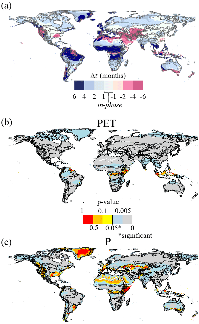
Figure 1Global spatial distributions of Δt (a) and of performance of monthly P (b) and PET (c) sine fits represented by p value.
Figure 1a shows the overall global distribution of Δt (Eq. S1), where some banding around the tropics as well as the Middle East can be seen. Equation (1) yielded overall good fits to the long-term mean monthly distributions of P and PET, with and 0.84±0.18, respectively (mean ± standard deviation across all pixels). These sine fits to monthly PET were statistically significant (p value ≤0.05) in 97 % of pixels, while fits to monthly P were statistically significant in 85 % of pixels (Fig. 1b and c). Cumulative distribution functions of both R2 and p value for PET and P sine fits can be seen in Fig. S5 in the Supplement. Similarly to Berghuijs and Woods (2016), P fits were good in South America and not as good in parts of the Sahara (Fig. 1c). Our P fits were good in East Asia and not as good in the southern United States, while Berghuijs and Woods (2016) had more error in East Asia and less error in the United States. Lastly, compared to the performance of our PET fits shown in Fig. 1b, the temperature fits of Berghuijs and Woods (2016) were overall much less spatially homogeneous than ours.
2.4 Established climate classification systems
Four previously established climate classification schemes were assessed in this analysis. We included two legacy schemes, Köppen–Geiger (KPG, Beck et al., 2018) and Holdridge life (HDL, Holdridge, 1967) zoning systems, and two recently proposed frameworks, here referred to as Meybeck Hydroregion (MHR, Meybeck et al., 2013) and Knoben Hydroclimate (KHC, Knoben et al., 2018) systems. Note that the original KHC zones created by Knoben et al. (2018) were not delineated by discrete boundaries but were instead represented as pixels with a corresponding probability continuum of belonging to a zone. However, Knoben et al. (2018) chose to bound 18 zones using their provided climate indices (aridity index, seasonal aridity index, and precipitation as snow) for inter-system comparison purposes. In the present study, 18 KHC boundaries were re-created using those climate indices in a clustering approach similar to the clustering methodology of Knoben et al. (2018). Here we applied a k-means, multi-start clustering method (n=80 starts), which was also used to form boundaries in two of our proposed frameworks described below. This k-means clustering approach, based on the Hartigan and Wong (1979) algorithm, was employed using the kmeans function in R package stats (R Core Team, 2018). Note that the very small KPG zones “Csc” and “Cwc” did not appear in the resolution KPG output created by Beck et al. (2018) that was used in this study, resulting in 28 KPG presently analyzed zones. As in other climate classification studies (Knoben et al., 2018; Meybeck et al., 2013), KPG was considered here to be the standard to which other systems are primarily compared and evaluated for performance.
2.5 Novel univariate ET climate classification systems
This study establishes and verifies ET-relevant climate classification frameworks by creating zones primarily based on ET rates and comparing ET coherence between systems. Three of the four systems developed in this study were univariate (formatted from global mean annual ET rates) with a single condition to emphasize a specific optimization goal. A fourth multivariate system is described below.
The first two novel univariate classification systems were based on the empirical cumulative distribution function (CDF) for global long-term mean annual ET rates. The first classification system, ET Area-optimizing (ETA), was created with the condition of having nearly equal area in each ET-based zone. This was motivated by the first complexity principle described in Sect. 2.1, which states that zones should not be meaninglessly small or disproportionately large. The KPG system has relatively high spatial non-uniformity, resulting in highly variable relevance for regional analyses. A classification system that is more spatially uniform can better inform large-spatial-scale understanding as well as the application of regional to semi-continental management strategies. Additionally, it is useful to have a simple baseline framework upon which to compare the other ET-based systems. Ultimately, ETA is a system that seeks to maximize area efficiency. This type of spatial condition is similar to the prioritizations of the MHR framework that suggest zones should ideally be “delineated in one piece,” although this is not a physical reality (Meybeck et al., 2013). The cumulative probability interval [0, 1] was divided into 15 equal parts, each corresponding to a separate zone, and the upper and lower bounds of ET thresholds for each zone were determined from the CDF of mean annual ET for all global land pixels (Fig. S6A in the Supplement). The number of ETA zones was chosen based on the number of zones in previously established systems and the relative improvement of ET coherence with the addition of more zones (Fig. S6B).
The second proposed classification system, ET Variability-optimizing (ETV), was based on the principle of maximizing within-zone ET coherence subject to the tradeoff of increasing complexity by adding zones. By fitting the empirical CDF with a continuous distribution, zone boundaries can be determined analytically for a minimum desired CVmin. For simplicity, and supported by empirical evidence (Fig. S7 in the Supplement), we fitted a uniform distribution, which is characterized by lower and upper bounds a and b, with . The ET limits defining each zone, i, were then determined directly from this relation as
where the upper and lower limits of sequential zones are shared (i.e., ). The largest value of b=1454 mm yr−1 was based on the maximum ET for all pixels, and CVmin=0.075 was chosen based on marginal CV decrease with an increasing number of zones (Fig. S7-B), which resulted in 29 zones. This method produces nearly equal CVs in all zones. Corresponding ET limits for each zone are shown in Fig. S7-A.
The third univariate scheme proposed here is the ET Clustering (ETC) classification system, in which the k-means clustering approach was applied. Previous analyses have used clustering techniques for climate classification purposes (Tapiador et al., 2019), including for the construction of the KHC boundaries (Knoben et al., 2018). Zones were built using a multi-start framework (n=80 starts) by forming clustering centers iteratively until the within-zone sum of squares of mean annual ET, based on Euclidean distances, was reduced. This method encompasses aspects of both ETA and ETV, in which ET variability and area distribution are considered. The ETC approach serves to compare a clustering methodology against the previously described analytical ET-based zoning frameworks. The final number of 20 clustering centers (i.e., zones) was selected based on the smallest number of zones with CV of mean annual ET below a low threshold, selected here as 0.1 (Fig. S8 in the Supplement).
2.6 Novel multivariate climate classification system
The final system developed in this study is a multivariate climate clustering framework, which was created from the same k-means clustering method described for the ETC framework. This new climate classification system included two hydroclimate variables (mean annual P and PET) and was designed for comparison against the univariate ET classification frameworks as well as previously established systems that were similarly formed from multiple variables. This final system is herein referred to as the Water-Energy Clustering (WEC) climate classification system.
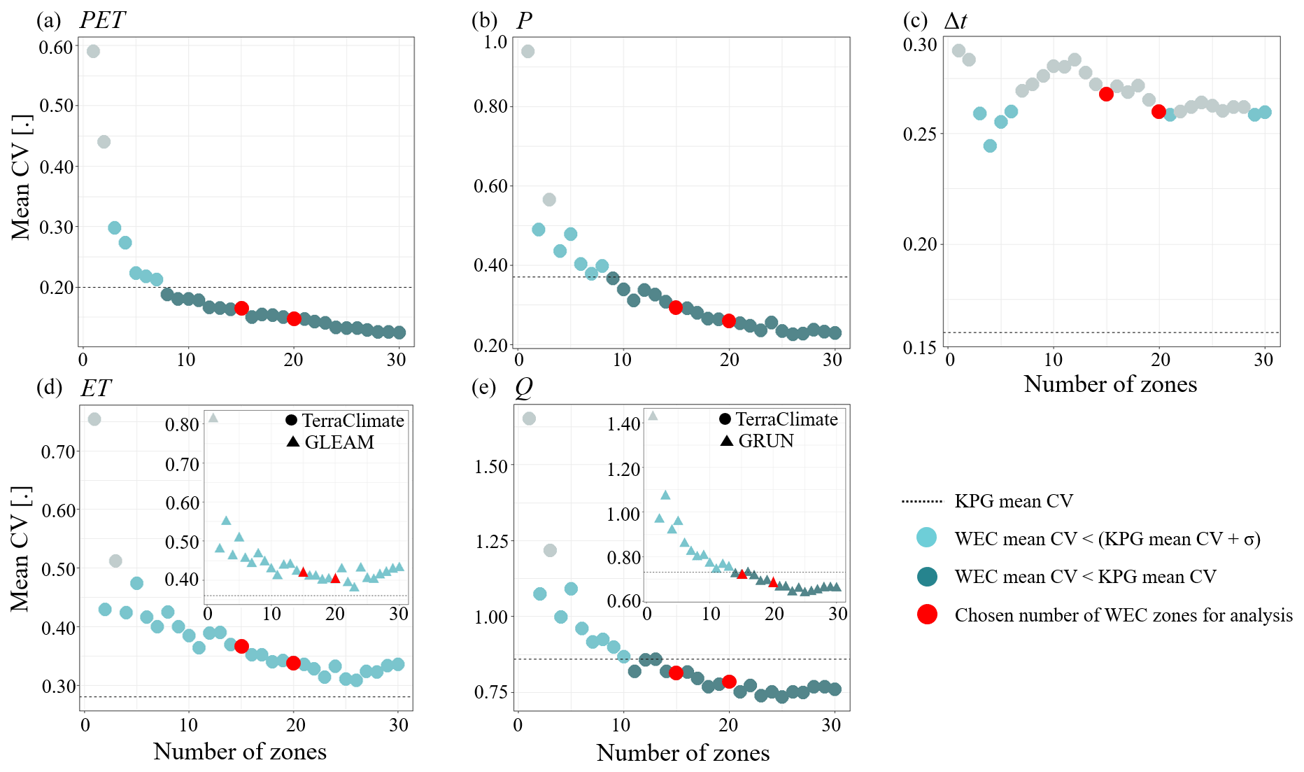
Figure 2Hydroclimate coherence with respect to number of possible zones within the WEC framework for all hydroclimate variables: PET (a), P (b), Δt (c), ET (d), and Q (e). For independent validation, ET and Q are also included from secondary gridded data sources, GLEAM and GRUN, respectively, and are differentially illustrated by triangles. Number of zones that yielded a mean CV value lower than that of KPG (gridded horizontal line) are shown in dark blue, number of zones that yielded a mean CV value that was lower than that of KPG plus 1 standard deviation (σ) are shown in light blue, number of zones that yielded a mean CV value that was higher than that of KPG plus σ are shown in light grey, and the final number of zones chosen for further evaluation are in red.
Since the KPG is the standard framework to which other systems were compared, a main objective was to create a classification scheme that was at least as good as KPG while also using fewer biophysical parameters to draw zone boundaries. The final number of proposed WEC zones was chosen based on the common “elbow method” for visually determining the optimal number of clusters, or zones (Syakur et al., 2018). Within the context of the presently applied k-means clustering method, the elbow method seeks to efficiently minimize the total within-zone sum of squares (TSS), such that the optimal number of zones exists where the rate of TSS change starts to decrease with the addition of more zones. According to the goal of efficiently minimizing the TSS, about five zones would be best (Fig. S9 in the Supplement). However, the aim of this study was to optimize zones based on hydroclimate coherence and zone shape complexity. Considering this premise, the “elbow” of hydroclimate coherence (i.e., low CV values) with respect to number of zones was between 10 and 20 zones for all hydroclimate variables, except for Δt (Fig. 2). Similarly, the elbow denoting the efficient minimization of mean number of patches across zones was approximately 15 to 25 WEC zones, but CV of zone area was relatively constant between 10 and 30 zones (Fig. S10B in the Supplement). A WEC system comprising at least 10 zones yielded mean coherence values that were better than those of KPG for PET, P, and Q, as denoted by dark blue dots in Fig. 2. It should also be noted that although there was no number of WEC zones that provided a lower mean number of patches than KPG, most possible numbers of WEC zones yielded mean values that were within 1 standard deviation of the KPG mean (Fig. S10A). Also, all possible numbers of WEC zones allowed for a more equal distribution of zone areas compared to the CV of zone area for KPG (Fig. S10B). We evaluated both 15 and 20 possible WEC zones (compared to KPG's 30-zone system) against all climate classification systems. However, the results for 15 WEC zones will be presented henceforth, since the K–S test showed no statistical difference in coherence or complexity between 15 and 20 zones (the coherence and complexity results for 20 WEC zones can be seen in Table S1 in the Supplement).
This study compared four previously established climate classification systems (KPG, HDL, MHR, and KHC) and four potential new climate classification systems (ETA, ETV, ETC, and WEC) to assess hydroclimate coherence as well as zone boundary complexities. The coherence of hydroclimate variables, PET, P, Δt, and TerraClimate ET and Q for each evaluated climate classification system is shown in Fig. 3. Figure S11 in the Supplement illustrates the coherence of GLEAM ET and GRUN Q, which were variables used to augment independent validation. A two-sided K–S test was conducted to determine differences between the cumulative distributions of CVs compared to a reference system for each variable. The WEC system was used as the reference system, since WEC is the novel multivariate system proposed in this study.
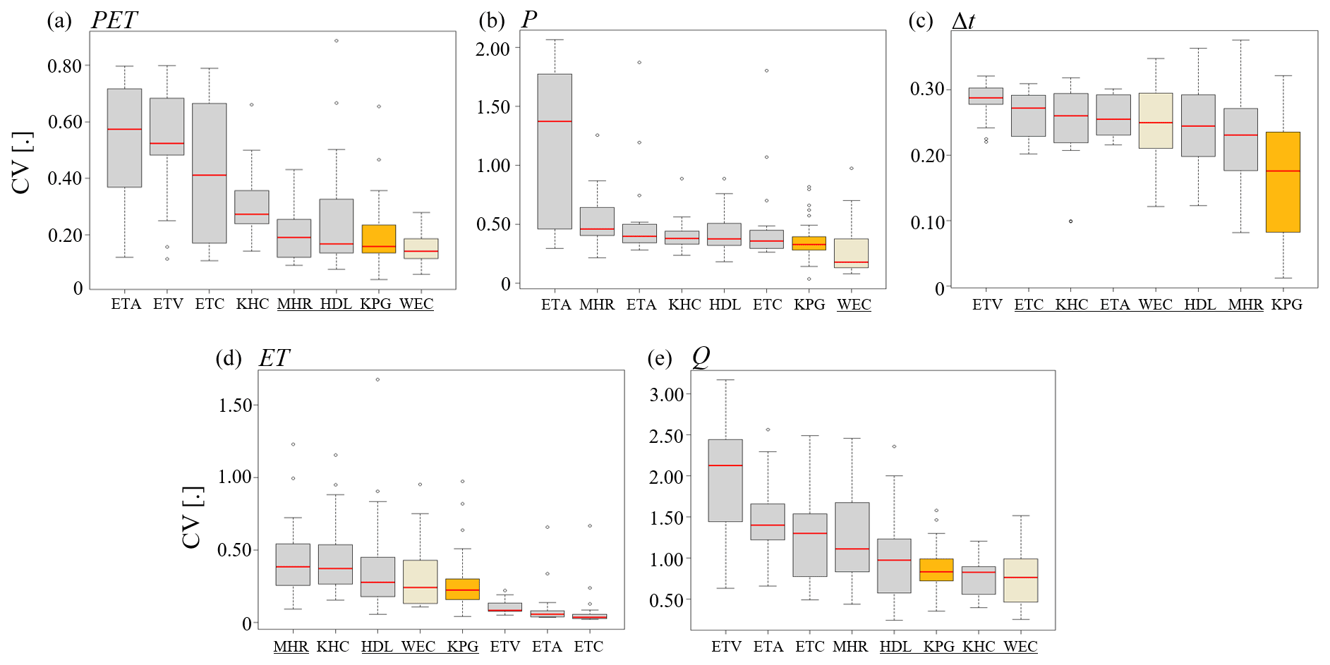
Figure 3Boxplots of coherence, quantified as intra-zone CV for hydroclimate variables of interest (a–e), for each assessed climate classification system. In each panel, KPG is shown in gold and WEC in light beige. The K–S test was used to determine whether the distributions were different from WEC. Systems whose coherence distributions were not statistically different from that of WEC are underlined.
Figure 4 showed MHR was the least fragmented system overall, although the KPG system was also characterized by low patchiness when compared to the distributions of the other systems (Fig. 4a). The KPG system also had relatively high hydroclimate coherence for most variables, including validation datasets GLEAM ET and GRUN Q (Fig. S11), appearing as the best system (i.e., low CV values) for Δt and not statistically different from the best system for PET and Q (Fig. 3). However, it did not have the highest P or ET coherence. The high Δt coherence of KPG is sensible, because KPG zones are built using intra-annual P and temperature (i.e., PET) dynamics. While the KPG system showed overall high coherence, which supports its status as the most widely used climate classification system, it was not the highest for all variables, and it also exhibited high complexity with respect to zone area distribution and number of zones used in its framework (Fig. 4b and c). Lastly, the number of biophysical parameters required to construct KPG zone boundaries (monthly P and temperature, n=24) is much higher than the novel systems presented here (n=2 for WEC and n=1, mean annual ET, for ETA-based systems).
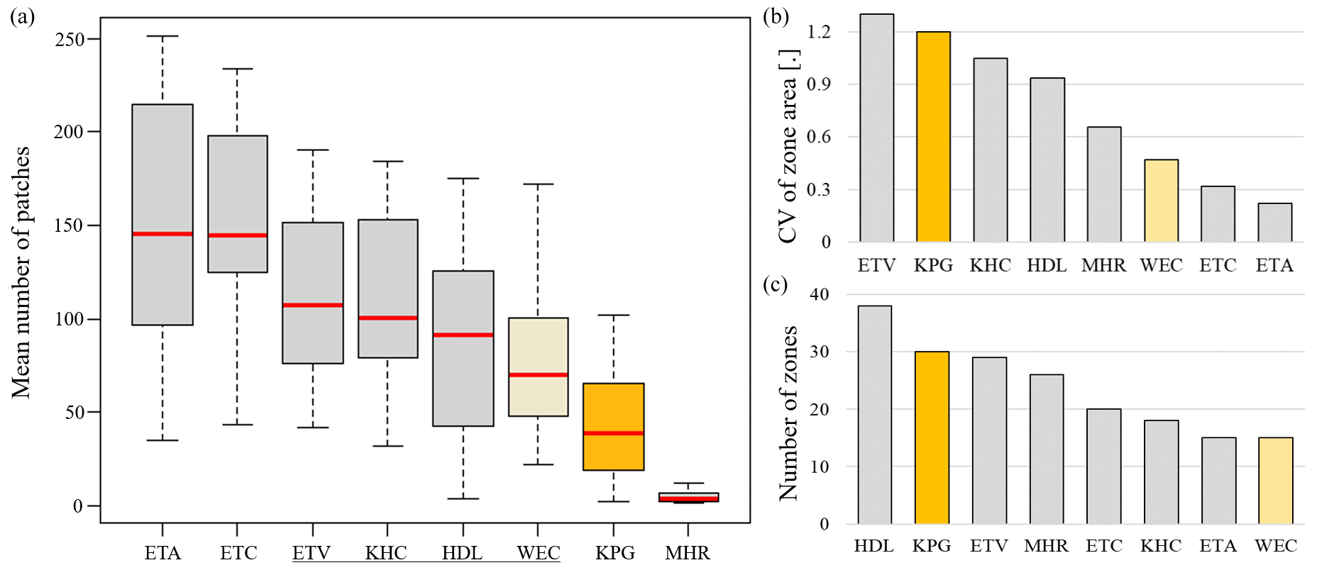
Figure 4Boxplots of mean number of patches per zone (a), barplots of CV of zone areas (b), and barplots of number of constructed zones (c) for each assessed climate classification system, with KPG shown in gold and WEC in light beige. The results of the K–S test were used to determine statistical difference of distributions compared to WEC. Systems whose distributions of mean number of patches were not statistically different from that of WEC are underlined.
The coherence of hydroclimate drivers, PET, P, and Δt, as well as hydroclimate response variables, ET and Q, were variable across systems (Fig. 3). The variable that was overall least coherent was Q (Figs. 3e and S11B), with both TerraClimate and GRUN Q CV values ranging beyond 1.50 for most classification systems, while the variable that was generally most coherent was Δt (Fig. 3c), with CV values generally between 0.10 and 0.30 for all assessed classification systems. Of all variables, Δt yielded the greatest number of systems not statistically different from WEC, based on the K–S test for differences in CV distributions (Fig. 3c). Additionally, the three novel ETA, ETV, and ETC systems had better ET coherence than the other classification systems (Fig. 3d). The ETA system, along with WEC, also had the fewest number of zones and provided the most uniform zone size distribution (Fig. 4b and c) but was not as coherent with respect to hydroclimate variables apart from ET (Fig. 3).
The WEC system had the lowest median CV for PET, P, and both TerraClimate Q (Fig. 3a, b, and e) and GRUN Q (Fig. S11B). It is reasonable that the WEC system is the most PET and P coherent, since these were the variables used to form the zone boundaries of the system. The high coherence of GRUN Q serves as an independent validation of the WEC framework, such that it can be concluded that the WEC system most effectively bounds zones that capture water availability drivers. Although the ET-based systems were best at bounding within-zone ET similarities and yielding high coherence, WEC did not perform worse than KPG in ET coherence, according to the K–S test (Fig. 3d). The WEC system was also relatively less complex compared to most other systems, including KPG, with respect to zone area distribution and number of zones required to draw hydroclimatically coherent boundaries (Fig. 4b and c). The WEC distribution of the mean number of patches in each zone was statistically different from that of KPG, and the WEC system had the next lowest median value following KPG (Fig. 4a). Since the proposed WEC system had similar or better performance than the KPG system in coherence and complexity metrics (except for Δt coherence and mean number of patches) and required 2 compared to 24 parameters to construct, the evaluated WEC framework was selected as the overall best hydroclimate classification system.
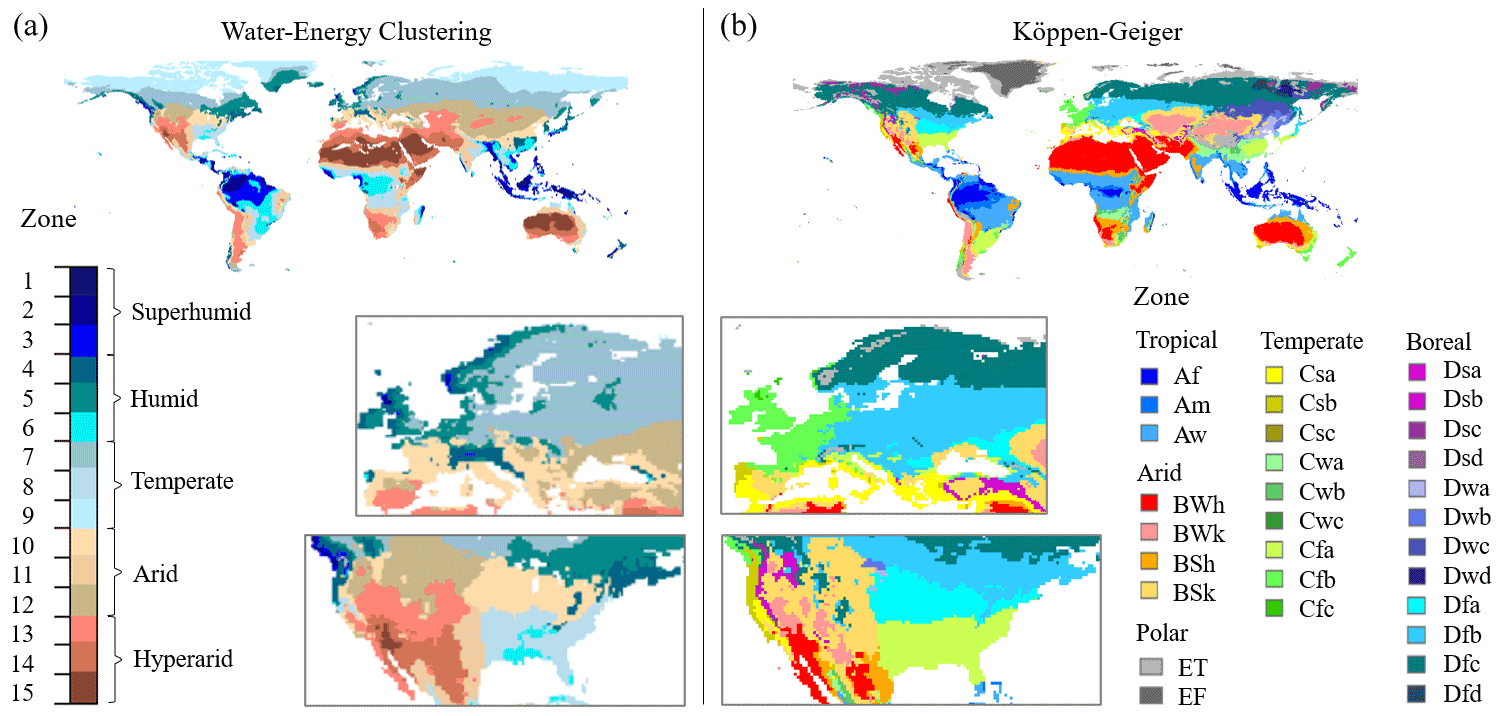
Figure 5Spatial distribution of WEC (a) and KPG (b) classification systems. Europe and North America are magnified.
The KPG system qualitatively groups 30 zones into five primary categories (“Tropical”, “Arid”, “Temperate”, “Boreal”, and “Polar”), and here the 15 WEC zones were also divided into five primary groups by ranking zones based on increasing zone mean aridity index, , where brackets indicate the spatial average within a zone and is the mean across zones within a group. The ranked zones were evenly grouped into the five categories: “Superhumid” (, “Humid” (, “Temperate” (, “Arid” (, and “Hyperarid” (. Note that the single WEC zone with the highest aridity encompasses the Sahara, parts of Saudi Arabia, and western Australia, for which φ=14.8. Maps of the boundaries for the proposed WEC system and the standard KPG framework are compared in Fig. 5. While there were some spatial similarities (e.g., see the Iberian Peninsula in Fig. 5), most regions were divided differently. For example, parts of northern Europe were mainly divided into three KPG zones but four WEC zones. Similarly, the southeastern United States, excluding southern Florida, was mostly one KPG zone but was separated in the WEC system into two distinct zones. The KPG framework conversely divided eastern and western Europe into respective temperate and boreal zones, while WEC treated western Europe as more heterogeneous. Clustering centers, which are the arithmetic means of each of the clusters, for the WEC climate classification system are listed in Table S2 in the Supplement.
We hypothesized that variable coherence and zone shape complexity would be related to the governing principles of the classification systems, which was mostly supported by the results of this study. For example, the principle of contiguity in the MHR system led to the lowest patchiness of all systems evaluated, so this system could be useful when continuous boundaries are important for ease of implementation or interpretation purposes. Additionally, concordant with the objectives of each ET-based framework, the three univariate ET-based classification systems had the highest ET coherence, while ETA (which additionally optimized equal zone area) also had the most uniform area distribution across zones. The KPG framework had the overall highest Δt coherence of the eight total compared systems, which is reasonable since KPG was the only system that accounted for monthly variability of water (P) and energy (temperature), which results in 24 biophysical parameters (Beck et al., 2018). The KHC framework similarly accounted for the long-term mean monthly ratio of P and PET, but it was not particularly high in Δt coherence (Fig. 3c). The WEC system was also based on water (P) and energy (PET) but from a mean annual perspective, thus requiring only two biophysical parameters as input variables. It is important to highlight that all novel systems presented here required fewer input variables, a notable aspect of system complexity, than any other evaluated previously established climate classification system, and substantially fewer than KPG.
Of the four previously established systems, KPG was the most hydroclimatically coherent but had high zone area variability (Fig. S10), even with the omission of the two small KPG zones when resampled to resolution in this study. When comparing all eight systems, WEC had the highest P, PET, and Q coherence and similar ET coherence to KPG. Although it was not surprising that the WEC classification systems yielded the highest P and PET coherence, given these were the variables used to draw its zone boundaries, WEC also had much more uniform zone area distribution, half the number of zones, and required substantially fewer parameters when compared to KPG. Areas of similar water availability rates, as defined by a low CV of Q, were best delineated by WEC, given that this system yielded the highest coherence for both TerraClimate Q and the independent validation source, GRUN Q. The MHR system used the long-term mean Q as a governing principle (Meybeck et al., 2013), while the KHC framework considered the Q regime as independent validation for their zones (Knoben et al., 2018). Although the MHR system used mean annual Q in their framework, it was not comparatively high in mean annual Q coherence, perhaps because their relatively larger zones did not reduce within-zone Q variability as much or because the present analysis considers locally generated Q (P–ET) and not gauged streamflow as they did. However, the KHC framework used gauged streamflow data for system evaluation (Knoben et al., 2018), and this system yielded a distribution of CV of Q not statistically different from that of WEC, which yielded the lowest median CV of Q.
Optimizing ET variability was a previously unconsidered objective in creating and validating climate classification schemes. The climate classification system comparison presented here supports the longstanding assertion that the primary mean ET drivers, water and energy (i.e., P and PET), are important considerations for broad hydroclimate analyses. For example, to delineate the landscape based on ET dynamics, the Budyko framework is a well-vetted mechanism for estimating the evaporative index (ET) using the primary drivers of the water budget, PET and P, as represented by the aridity index (Budyko, 1974; Milly, 1994; Reaver et al., 2020a, b; Zhang et al., 2004). We conclude that hydroclimate coherence is best achieved when P and PET are the governing principles of a zoning framework. However, when specifically evaluating ET dynamics, applying an ET-based delineation could be useful, especially if the objective of such a study is to distinctively evaluate factors that influence ET. It should be noted that boundaries created by ET drivers and not ET rates may influence the determined importance of such drivers, since intra-zone driver variability is likely to be reduced. Based on both ET coherence and spatial complexity, the ETA system established here is suggested for ET-focused questions such as large-scale assessments of ET drivers or crop productivity (Howell et al., 2015).
This study is limited by a few factors. First, distinct climate zone boundaries, although useful in practice, do not exist in the physical system (Knoben et al., 2018). Second, this study compared averaged metrics that were applied across zones within each classification system and did not distinguish between individual zones, which could be evaluated in subsequent studies. Third, the focus on long-term mean annual hydroclimate attributes for zone formation does not account for interdecadal climate dynamics. Last, the TerraClimate ET and Q data used to assess the suite of classification systems were in part formed using the same CRU climate data used here to create the WEC boundaries (Abatzoglou et al., 2018). However, GLEAM ET and GRUN Q were also used as independent datasets and did not yield different results, which is likely due to two primary reasons: (1) the spatial scope of this analysis is sufficiently large, such that calibrated rates for all hydroclimate variables are regionally representative (Abatzoglou et al., 2018), and (2) similarly, long-term hydrologic dynamics are not as subject to interannual variability, since these effects are more muted across longer timescales. In this way, the broad spatiotemporal nature of this analysis makes it reasonable that all available P, ET, Q, and PET data are appropriate metrics for forming more robust hydroclimate boundaries and subsequently assessing the water and energy budgets therein.
The KPG system is the most widely used climate classification system, and this analysis revealed that it indeed has relatively high hydroclimatic coherence with respect to several variables, but it also has high spatial complexity, as evidenced by multiple metrics in addition to its 24-parameter requirement. It was concluded that WEC was either better than or not statistically different from all other previously established systems, including the KPG framework, in all assessed coherence metrics apart from Δt. Moreover, compared to KPG, WEC builds half the number of zones using only two parameters as input variables and delineates a more uniform zone area distribution to better facilitate meaningful spatial interpretations.
It is widely accepted that water and energy, chiefly in the form of precipitation and solar radiation, govern long-term socioecological water availability at large spatiotemporal scales (Budyko, 1974; Berghuijs and Woods, 2016; Knoben et al., 2018; Sanford and Selnick, 2013). Several previous climate classification systems aimed to represent this water–energy interaction within bounded zones that encompass similar hydroclimatic sensitivities (Knoben et al., 2018; Meybeck et al., 2013). It was concluded here that WEC, using water and energy in the form of P and PET rates, was the best overall system for building zones that encompass similar Q rates. This suggests that the WEC scheme is valuable for assessing and predicting water availability changes given changes in water and energy. Therefore, WEC is the most relevant system for direct management understanding and application as it relates to hydroclimate dynamics.
This study proposes WEC as a new framework for regional hydroclimate inquiries and other large-spatial-scale research endeavors that may be influenced by hydroclimate systems that vary across the landscape. The WEC system is robust, since it is based on long-term mean annual rates that have low susceptibility to interannual and seasonal variability. This work is a promising pathway to regionalization within many different biophysical and socioeconomic contexts, clustering drivers to form zones of similar response variable sensitivities in order to more accurately extrapolate locally derived results and regional impacts of local management practices. The WEC framework can thus inform regional- to national-scale management strategies in the effort to account for potential hydroclimate zone-dependent responses to climate and land cover changes.
The code used in this study is available at https://doi.org/10.5281/zenodo.5748255 (Pisarello and Jawitz, 2021).
Netcdf files for the proposed WEC and ETA classification systems are available at the link above under “Code availability” (Pisarello and Jawitz, 2021). All data used in this study are publicly accessible, with noted descriptions in Sect. 2.2 “Database construction”. Climate Research Unit TimeSeries V4.04 (Harris et al., 2020) can be retrieved from the online catalog (https://catalogue.ceda.ac.uk/uuid/89e1e34ec3554dc98594a5732622bce9, University of East Anglia Climatic Research Unit et al., 2020). The following open-access data can be found: TerraClimate: https://www.climatologylab.org/terraclimate.html (Climatology Lab, 2021), GLEAM: https://www.gleam.eu/#downloads (Martens et al., 2017; Miralles et al., 2011), GRUN: https://doi.org/10.6084/m9.figshare.9228176 (Ghiggi et al., 2019).
The supplement related to this article is available online at: https://doi.org/10.5194/hess-25-6173-2021-supplement.
KLMP performed the analyses and led the manuscript preparation. JWJ conceived and directed the study.
The contact author has declared that neither they nor their co-author has any competing interests.
Publisher's note: Copernicus Publications remains neutral with regard to jurisdictional claims in published maps and institutional affiliations.
This research was supported in part by USDA National Institute of Food and Agriculture Hatch project FLA-SWS-005461. James W. Jawitz was supported in part by the National Science Foundation under award number 2000649.
This paper was edited by Roger Moussa and reviewed by four anonymous referees.
Abatzoglou, J. T., Dobrowski, S. Z., Parks, S. A., and Hegewisch, K. C.: TerraClimate, a high resolution global dataset of monthly climate and climatic water balance from 1958–2015, Scientific Data, 5, 170191, https://doi.org/10.1038/sdata.2017.191, 2018.
Beck, H. E., Zimmermann, N. E., McVicar, T. R., Vergopolan, N., Berg, A., and Wood, E. F.: Present and future Köppen Geiger climate classification maps at 1 km resolution, Scientific Data, 5, 180214, https://doi.org/10.1038/sdata.2018.214, 2018.
Berghuijs, W. R. and Woods, R. A.: A simple framework to quantitatively describe monthly precipitation and temperature climatology, Int. J. Climatol., 36, 3161–3174, 2016.
Bivand, R., Pebesma, E., and Gomez-Rubio, V.: Applied Spatial Data Analysis with R, 2nd edn., Springer, NY, 2013.
Boland, M. R., Parhi, P., Gentine, P., and Tatonetti, N. P.: Climate classification is an important factor in assessing quality-of-care across hospitals, Sci. Rep.-UK, 7, 1–6, 2017.
Budyko, M. I.: Climate and Life, Academic Press, New York, 1974.
Chen, D. and Chen, H. W.: Using the Köppen classification to quantify climate variation and change: An example for 1901–2010, Environmental Development, 6, 69–79, 2013.
Climatology Lab: TerraClimate, available at: https://www.climatologylab.org/terraclimate.html, last access: 1 December 2021.
Ghiggi, G., Humphrey, V., Seneviratne, S. I., and Gudmundsson, L.: GRUN: an observation-based global gridded runoff dataset from 1902 to 2014, Earth Syst. Sci. Data, 11, 1655–1674, https://doi.org/10.5194/essd-11-1655-2019, 2019.
Ghiggi, G., Gudmundsson, L., and Humphrey, V.: G-RUN: Global Runoff Reconstruction figshare [data set], https://doi.org/10.6084/m9.figshare.9228176.v2, 2019.
Guan, Y., Lu, H., He, L., Adhikari, H., Pellikka, P., Maeda, E., and Heiskanen, J.: Intensification of the dispersion of the global climatic landscape and its potential as a new climate change indicator, Environ. Res. Lett., 15, 114032, https://doi.org/10.1088/1748-9326/aba2a7, 2020.
Harris, I., Osborn, T. J., Jones, P., and Lister, D.: Version 4 of the CRU TS monthly high resolution gridded multivariate climate dataset, Scientific Data, 7, 1–18, 2020.
Hartigan, J. A. and Wong, M. A.: Algorithm AS 136: A k-means clustering algorithm, J. Roy. Stat. Soc. C-Appl., 28, 100–108, 1979.
Hesselbarth, M. H., Sciaini, M., With, K. A., Wiegand, K., and Nowosad, J.: landscapemetrics: an open-source R tool to calculate landscape metrics, Ecography, 42, 1648–1657, 2019.
Hijmans, R. J.: raster: Geographic Data Analysis and Modeling, R package version 3.4-13, available at: https://CRAN.R-project.org/package=raster, last access: 2 December 2021.
Holdridge, L. R.: Life Zone Ecology, Tropical Science Center, San Jose, Costa Rica, 1967.
Howell, T. A., Evett, S. R., Tolk, J. A., Copeland, K. S., and Marek, T. H.: Evapotranspiration, water productivity and crop coefficients for irrigated sunflower in the US Southern High Plains, Agr. Water Manage., 162, 33–46, 2015.
Jagai, J. S., Castronovo, D. A., and Naumova, E. N.: The use of Köppen climate classification system for public health research, Epidemiology, 18, S30, https://doi.org/10.1097/01.ede.0000276508.75400.ab, 2007.
Knoben, W. J., Woods, R. A., and Freer, J. E.: A Quantitative Hydrological Climate Classification Evaluated With Independent Streamflow Data, Water Resour. Res., 54, 5088–5109, 2018.
Lanfredi, M., Coluzzi, R., Imbrenda, V., Macchiato, M., and Simoniello, T.: Analyzing Space–Time Coherence in Precipitation Seasonality across Different European Climates, Remote Sens.-Basel, 12, 171, https://doi.org/10.3390/rs12010171, 2020.
Lloyd, S. J., Kovats, R. S., and Armstrong, B. G.: Global diarrhea morbidity, weather and climate, Clim. Res., 34, 119–127, 2007.
Magarey, R. D., Borchert, D. M., and Schlegel, J. W.: Global plant hardiness zones for phytosanitary risk analysis, Sci. Agric., 65, 54–59, 2008.
Martens, B., Miralles, D. G., Lievens, H., van der Schalie, R., de Jeu, R. A. M., Fernández-Prieto, D., Beck, H. E., Dorigo, W. A., and Verhoest, N. E. C.: GLEAM v3: satellite-based land evaporation and root-zone soil moisture, Geosci. Model Dev., 10, 1903–1925, https://doi.org/10.5194/gmd-10-1903-2017, 2017 (data available at: https://www.gleam.eu/#downloads, last access: 21 April 2021).
McKenney, D. W., Pedlar, J. H., Lawrence, K., Campbell, K., and Hutchinson, M. F.: Beyond traditional hardiness zones: using climate envelopes to map plant range limits, BioScience, 57, 929–937, 2007.
Mellinger, A., Sachs, J. D., and Gallup, J.: Climate, Coastal Proximity, and Development, 169–194, in: Oxford Handbook of Economic Geography, edited by: Clark, G. L., Feldman, M. P., and Gertler, M. S., Oxford University Press, New York, 2000.
Meybeck, M., Kummu, M., and Dürr, H. H.: Global hydrobelts and hydroregions: improved reporting scale for water-related issues?, Hydrol. Earth Syst. Sci., 17, 1093–1111, https://doi.org/10.5194/hess-17-1093-2013, 2013.
Milly, P. C. D.: Climate, soil water storage, and the average annual water balance, Water Resour. Res., 30, 2143–2156, 1994.
Miralles, D. G., Holmes, T. R. H., De Jeu, R. A. M., Gash, J. H., Meesters, A. G. C. A., and Dolman, A. J.: Global land-surface evaporation estimated from satellite-based observations, Hydrol. Earth Syst. Sci., 15, 453–469, https://doi.org/10.5194/hess-15-453-2011, 2011 (data available at: https://www.gleam.eu/#downloads, last access: 21 April 2021).
O'Neill, R. V., Krummel, J. R., Gardner, R. E. A., Sugihara, G., Jackson, B., and DeAngelis, D. L.: Indices of landscape pattern, Landscape Ecol., 1, 153–162, 1988.
Olson, D. M., Dinerstein, E., Wikramanayake, E. D., Burgess, N. D., Powell, G. V., and Underwood: Terrestrial Ecoregions of the World: A New Map of Life on Earth, A new global map of terrestrial ecoregions provides an innovative tool for conserving biodiversity, BioScience, 51, 933–938, 2001.
Papagiannopoulou, C., Miralles, D. G., Demuzere, M., Verhoest, N. E. C., and Waegeman, W.: Global hydro-climatic biomes identified via multitask learning, Geosci. Model Dev., 11, 4139–4153, https://doi.org/10.5194/gmd-11-4139-2018, 2018.
Peel, M. C., Finlayson, B. L., and McMahon, T. A.: Updated world map of the Köppen-Geiger climate classification, Hydrol. Earth Syst. Sci., 11, 1633–1644, https://doi.org/10.5194/hess-11-1633-2007, 2007.
Pierce, D.: ncdf4: Interface to Unidata netCDF (Version 4 or Earlier) Format Data Files, R package version 1.16, available at: https://CRAN.R-project.org/package=ncdf4 (last access: 2 December 2021), 2017.
Pisarello, K. and Jawitz, J.: ktpisa/Coherence-of-global-hydroclimate-classification-systems (v1.1.0c), Zenodo [code], https://doi.org/10.5281/zenodo.5748255, 2021.
R Core Team: R: A language and environment for statistical computing. R Foundation for Statistical Computing, Vienna, Austria, available at: https://www.R-project.org/ (last access: 1 October 2021), 2018.
Reaver, N. G. F., Kaplan, D. A., Klammler, H., and Jawitz, J. W.: Reinterpreting the Budyko Framework, Hydrol. Earth Syst. Sci. Discuss. [preprint], https://doi.org/10.5194/hess-2020-584, in review, 2020a.
Reaver, N. G. F., Kaplan, D. A., Klammler, H., and Jawitz, J. W.: Technical Note: Analytical Inversion of the Parametric Budyko Equations, Hydrol. Earth Syst. Sci. Discuss. [preprint], https://doi.org/10.5194/hess-2020-585, 2020b.
Richards, D., Masoudi, M., Oh, R. R., Yando, E. S., Zhang, J., and Friess, D. A.: Global Variation in Climate, Human Development, and Population Density Has Implications for Urban Ecosystem Services, Sustainability, 11, 6200, https://doi.org/10.3390/su11226200, 2019.
Sanford, W. E. and Selnick, D. L.: Estimation of evapotranspiration across the conterminous United States using a regression with climate and land-cover data 1, J. Am. Water Resour. As., 49, 217–230, 2013.
Syakur, M. A., Khotimah, B. K., Rochman, E. M. S., and Satoto, B. D.: Integration k-means clustering method and elbow method for identification of the best customer profile cluster, IOP Conference Series: Materials Science and Engineering, 336, 012017, https://doi.org/10.1088/1757-899X/336/1/012017, 2018.
Tapiador, F. J., Moreno, R., Navarro, A., Sánchez, J. L., and García-Ortega, E.: Climate classifications from regional and global climate models: Performances for present climate estimates and expected changes in the future at high spatial resolution, Atmos. Res., 228, 107–121, 2019.
University of East Anglia Climatic Research Unit, Harris, I. C., Jones, P. D., and Osborn, T.: CRU TS4.04: Climatic Research Unit (CRU) Time-Series (TS) version 4.04 of high-resolution gridded data of month-by-month variation in climate (Jan. 1901–Dec. 2019), Centre for Environmental Data Analysis [data set], available at: https://catalogue.ceda.ac.uk/uuid/89e1e34ec3554dc98594a5732622bce9, last access: 1 July 2020.
Zhang, K., Kimball, J. S., and Running, S. W.: A review of remote sensing based actual evapotranspiration estimation, WIREs Water, 3, 834–853, 2016.
Zhang, L., Hickel, K., Dawes, W. R., Chiew, F. H., Western, A. W., and Briggs, P. R.: A rational function approach for estimating mean annual evapotranspiration, Water Resour. Res., 40, W02502, https://doi.org/10.1029/2003WR002710, 2004.
The requested paper has a corresponding corrigendum published. Please read the corrigendum first before downloading the article.
- Article
(1294 KB) - Full-text XML
- Corrigendum
-
Supplement
(1308 KB) - BibTeX
- EndNote