the Creative Commons Attribution 4.0 License.
the Creative Commons Attribution 4.0 License.
 | 22 Nov 2021
Design flood estimation for global river networks based on machine learning models
Paul Bates
Jeffrey Neal
Bo Pang
Design flood estimation is a fundamental task in hydrology. In this research, we propose a machine-learning-based approach to estimate design floods globally. This approach involves three stages: (i) estimating at-site flood frequency curves for global gauging stations using the Anderson–Darling test and a Bayesian Markov chain Monte Carlo (MCMC) method; (ii) clustering these stations into subgroups using a K-means model based on 12 globally available catchment descriptors; and (iii) developing a regression model in each subgroup for regional design flood estimation using the same descriptors. A total of 11 793 stations globally were selected for model development, and three widely used regression models were compared for design flood estimation. The results showed that (1) the proposed approach achieved the highest accuracy for design flood estimation when using all 12 descriptors for clustering; and the performance of the regression was improved by considering more descriptors during training and validation; (2) a support vector machine regression provided the highest prediction performance amongst all regression models tested, with a root mean square normalised error of 0.708 for 100-year return period flood estimation; (3) 100-year design floods in tropical, arid, temperate, cold and polar climate zones could be reliably estimated (i.e. <±25 % error), with relative mean bias (RBIAS) values of −0.199, −0.233, −0.169, 0.179 and −0.091 respectively; (4) the machine-learning-based approach developed in this paper showed considerable improvement over the index-flood-based method introduced by Smith et al. (2015, https://doi.org/10.1002/2014WR015814) for design flood estimation at global scales; and (5) the average RBIAS in estimation is less than 18 % for 10-, 20-, 50- and 100-year design floods. We conclude that the proposed approach is a valid method to estimate design floods anywhere on the global river network, improving our prediction of the flood hazard, especially in ungauged areas.
- Article
(3694 KB) - Full-text XML
- BibTeX
- EndNote


Flood hazard is the primary weather-related disaster worldwide, affecting 2.3 billion people and causing USD 662 billion in economic damage between 1995 and 2015 (CRED and UNISDR, 2015). The frequency and severity of flood events are expected to increase in the future because of climate change and socio-economic growth in flood-prone areas (Sharma et al., 2018; Wing et al., 2018; Winsemius et al., 2016). Flood hazard models are mature tools to identify flood-prone areas and have been widely used in flood risk management at catchment or regional scales (Hammond et al., 2015; Teng et al., 2017). With the development of new remote sensing techniques and an increase in computing power, global flood hazard models (GFHMs) are now a practical reality and have been successfully applied for large-scale flood mapping and validated in several countries (Bates et al., 2020; Schumann et al., 2018). GFHMs can identify flood-prone areas in ungauged basins and provide a consistent and comprehensive understanding of the flood hazard at national, continental and global scales.
The “cascade” model type and “gauged flow data” model type are the two most frequently used approaches in global flood hazard modelling, and both map the flood hazard based on return period flows (Trigg et al., 2016). The cascade model type, for example CaMa-UT (Yamazaki et al., 2011) and GLOFRIS (Winsemius et al., 2013), uses land surface models driven by climate reanalysis data to simulate streamflow. Return period flows along the river network in the cascade model type are derived by an at-site flood frequency analysis of the resulting land surface model streamflow. However, due to the coarse resolution (usually 0.5∘) of global climate and land surface models (Yang et al., 2019b; Liu et al., 2019), some downscaling and bias correction methods usually need to be adopted for high-resolution flood hazard mapping (Müller Schmied et al., 2016; Frieler et al., 2017; Schumann et al., 2014a). Unlike the cascade model type, the gauged flow data model type uses observed gauged discharge and regional flood frequency analysis (RFFA) approaches to produce different return period flows along the global river network (Trigg et al., 2016). Compared with the cascade model type, the gauged flow data model type can be preferable for high-resolution flood hazard mapping as it avoids the uncertainties from rainfall-runoff modelling (Prihodko et al., 2008) and flood map downscaling (Schumann et al., 2014b). However, the performance of the RFFA approach adopted is highly dependent on the coverage and density of observed discharge stations (Hosking and Wallis, 1988; Lin and Chen, 2006).
RFFA has long been regarded as a reliable method to estimate design floods in engineering hydrology (Cunnane, 1988). Based on the basic assumption that there is a relationship between catchment descriptors and the design flood in a region, different types of RFFA approaches have been proposed and successfully applied in regional studies in the past 5 decades (Griffis and Stedinger, 2007; Merz and Blöschl, 2008a, b; Dalrymple, 1960). Among these, the index-flood method and the direct regression method are two of the most widely used procedures (Shu and Ouarda, 2008). The index-flood method assumes that the flood frequency curves at different sites in a region are identical except for one scale index (named the index flood) (Dalrymple, 1960; Bocchiola et al., 2003). Therefore, the index-flood method involves two steps, index-flood estimation and derivation of a single regional flood frequency relationship, often termed a growth curve. Unlike the index-flood method, the direct regression method predicts flood quantiles as a function of catchment descriptors directly (Shu and Ouarda, 2008). These two methods have been successfully applied at both regional and continental scales (Salinas et al., 2013), but very few applications of such methods have been performed at the global scale. To date, Smith et al. (2015) have proposed an RFFA approach at the global scale based on the index-flood method (termed global RFFA). This approach has been applied successfully in high-resolution flood hazard mapping for ungauged areas in several countries (Sampson et al., 2015; Wing et al., 2017).
However, the global RFFA approach of Smith et al. (2015) has shown some deficiencies during application, which we seek to address in this research as follows:
-
The global RFFA approach of Smith et al. (2015) was developed based on 945 stations in the Global Runoff Data Base (GRDB) and the United States Geological Survey (USGS) database. This limited number of stations means that it cannot provide a reliable estimation in some regions at global scale. To improve the coverage and density of discharge stations, nearly 12 000 stations from the newly published Global Streamflow Indices and Metadata (GSIM) archive were selected for model development in this research.
-
The flood frequency curve in the Smith et al. (2015) approach was assumed to obey a generalised extreme value (GEV) distribution for the global coverage. Studies have suggested alternate distributions, such as GEV, generalised logistic (GENLOGIS) and Pearson type III (P3), whilst log-normal (LN3) distributions are mandated for use in the United States (Water Resources Council (US), 1975). In this research, the at-site flood frequency curve was selected from eight widely used distributions based on the Anderson–Darling goodness-of-fit tests.
-
The global RFFA approach of Smith et al. (2015) adopted only three catchment descriptors (rainfall, slope and catchment area) for clustering and flood estimation. These three factors can only provide a basic description of global catchment characteristics. In this research, 12 catchment descriptors covering meteorological, physiographical, hydrological and anthropological aspects were considered for clustering and design flood estimation.
-
The global RFFA approach of Smith et al. (2015) was proposed based on the index-flood method, and the index flood in ungauged areas was computed with a power-form function. As the coefficient of variation of flood flows generally varies from site to site, the index-flood method is not recommended if available samples are sufficient or highly cross-correlated (Stedinger, 1983). Moreover, the simple power-form function may fail to capture complicated relationships within the data, since the relationship between flood and each descriptor is assumed to obey an explicit power-form function, which may not always be appropriate. In this research, the design flood in ungauged areas is estimated based on a direct regression method, and machine learning models were adopted to describe the unknown relationship between catchment descriptors and at-site design floods. These machine-learning-based methods have shown advantages over ordinary regression approaches in RFFA at regional scales (Gizaw and Gan, 2016; Shu and Ouarda, 2008; Zhang et al., 2018) and are tested here for the first time in a global study.
The aim of this research is therefore to provide an improved method for reliable design flood estimation, addressing the deficiencies identified with the previous global-scale study of Smith et al. (2015). A three-phase model framework is applied, where Bayesian Markov chain Monte Carlo (MCMC), K-means and support vector machine (SVM) models were applied for at-site flood estimation, subgroup delineation and regional flood estimation, respectively. Specifically, 11 793 stations selected from the GSIM archive are used for model development, and the stations were divided into 16 subgroups using a K-means model and 12 catchment descriptors. For each subgroup, 70 % and 30 % stations were randomly selected for model training and validation respectively. Three types of regressions including power-form function (PF), SVM and random forest (RF) were compared for regional flood estimation. Finally, the proposed direct regression approach is compared with the previous results of Smith et al. (2015) in each climate zone.
2.1 Flood data
Observed annual maximum streamflow data in the GSIM archive were used to estimate at-site design floods (DFs) at different return periods. This archive is a collection of streamflow indices that includes more than 35,000 stations from seven national and five international streamflow databases (Gudmundsson et al., 2018; Do et al., 2018a). Compared with a widely used database in large-scale hydrological studies, the Global River Discharge Database (GRDB), which contains data from 9500 stations, the GSIM archive can help to improve the understanding of large-scale hydrological processes by improving the coverage and density of streamflow observations. After quality control of the daily streamflow data, 15 types of time-series indices are provided at yearly, seasonal and monthly resolutions in the GSIM archive (Do et al., 2018a; Gudmundsson et al., 2018). In this research, time series of annual maximal floods in the GSIM archive were adopted for at-site design flood estimation. To date, this archive has been successfully used in flood classification (Stein et al., 2019), streamflow trend analysis (Do et al., 2019) and hydrological model evaluation (Yang et al., 2019a) at the global scale.
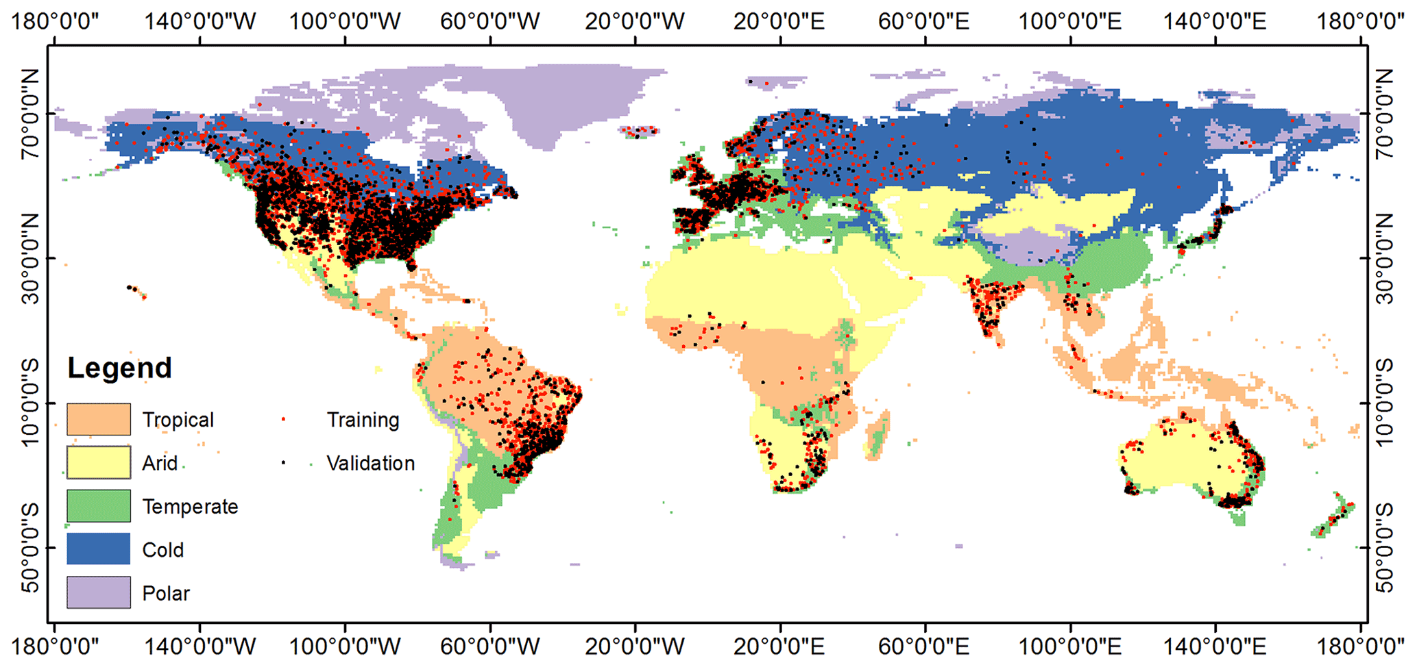
Figure 1The distribution of discharge stations used for training and validation in this research.
To make reliable estimates for at-site DFs, a station selection is needed based on some quality control criteria. Firstly, the hydrological signatures of streamflow are reported to become stable during estimation with at least 20 years of record (Richter et al., 1997). Therefore, only stations with a historical streamflow record of 20 years or longer were selected for the analysis. Second, the traditional RFFA approach requires the assumption of flood stationarity. Stations experiencing obvious trends or sudden changes were detected by a Mann–Kendall test (MKT) (Hamed, 2008) and the standard normal homogeneity test (SNHT) (Alexandersson, 1986). Any stations exhibiting obvious non-stationarity or which do not obey the given hypothetical distributions identified by Anderson–Darling goodness-of-fit tests were not considered further in model development. Lastly, to better estimate DFs at the global scale, the selected stations were first divided into several subgroups based on a K-means clustering model, and separate regression models were developed for the different subgroups. The streamflow stations in each subgroup were also required to pass discordancy and heterogeneity tests. The adopted stationarity, discordancy and heterogeneity measures are described in Sect. 3, and the distribution of training and validation stations after selection is shown in Fig. 1.
Table 1 compares the number of stations used for model training and validation in each climate class between Smith et al. (2015) and this study. Compared with the research of Smith et al. (2015), the number of stations in this research is significantly improved in all climate classes.
Table 1The number of discharge stations for model development in each climate class. NA stands for “not available”.

2.2 Catchment descriptors
The main idea of an RFFA is to characterise a relationship between at-site DFs and catchment descriptors and then apply this relationship to estimate flood magnitudes along the river network in similar ungauged catchments. In this research, the river network of the global coverage is extracted from the 1 km resolution catchment area map for catchments exceeding a threshold area of 50 km2. Twelve explanatory factors collected from open-access databases were selected as potential descriptors and applied for clustering and regression model development. A correlation analysis of all explanatory factors was done before model development to ensure none of them have strong correlation (Pearson's correlation coefficient > 0.6) with each other. The statistics and data sources of these factors are summarised in Table 2.
Table 2Statistics and data source of the explanatory descriptors.

These explanatory factors can be grouped into four categories as follows:
-
Meteorological factors included annual precipitation (AP), precipitation seasonality (PS), annual mean temperature (AT) and annual temperature range (TR). AP and AT represent the average annual precipitation and mean temperature of the upstream catchment respectively. PS is the coefficient of variation of the monthly rainfall series, and TR is the range between the maximal and minimal temperatures of the time series average over the upstream catchment. These four factors were collected from the WorldClim dataset (V2) at 30 arcsec (∼1 km) resolution (Fick and Hijmans, 2017) and are used to represent the extreme value and seasonal distribution of precipitation and temperature.
-
Physiographical factors comprised discharge station location, slope (SL) and lake fraction (LF) of the upstream catchment. Station location is defined by the longitude (LO) and latitude (LA) of the discharge station in degree units of the World Geodetic System 1984 (WGS84) spatial reference frame. SL reflects the average slope of the upstream catchment, which is calculated based on the MERIT DEM (Yamazaki et al., 2017). LF represents the fraction of the catchment area upstream of the station covered with lakes. The location and area of global lakes are taken from the Global Lakes and Wetlands Database (GLWD) (Lehner and Döll, 2004).
-
Hydrological factors of catchment area (CA) and curve number (CN) reflect the area and runoff capacity of the upstream catchment respectively. CA is defined as the upstream flow accumulation area based on the D8 algorithm and the MERIT DEM. CN is an empirical parameter for runoff prediction in ungauged areas, which is calculated from the tables in the National Engineering Handbook of the United States, Section-4 (NEH-4) (United States Soil Conservation Service, 1985). The CN in this research is collected from a global CN dataset that utilises the latest Moderate Resolution Imaging Spectroradiometer (MODIS) land cover information and the Harmonized World Soil Database (HWSD) soil data (Zeng et al., 2017).
-
Anthropological factors included total dam capacity (DC) and population density (PD). DC is the total dam capacity of the upstream catchment. The location and capacity of each dam are provided by the Global Reservoir and Dam (GRanD) dataset, which includes about 7000 dams globally (Lehner et al., 2011). PD is a widely used factor to reflect the impact of human activities on the environment. The PD map in this research is collected from the Gridded Population of the World (GPW) dataset of the year 2015 (Doxsey-Whitfield et al., 2015).
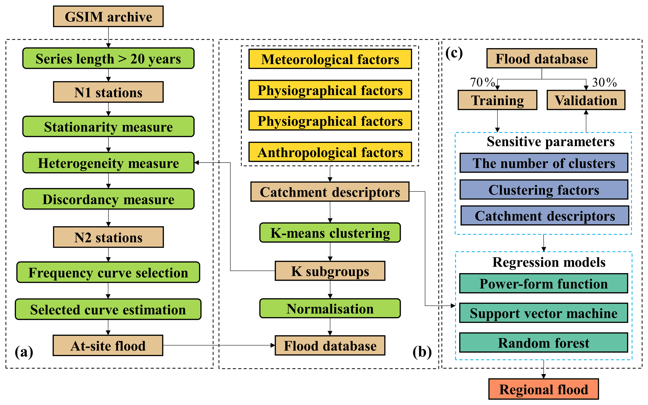
Figure 2The framework of this research. (a) At-site flood estimation; (b) subgroup delineation; (c) regional flood estimation.
The flowchart for this research has three parts, which are shown in Fig. 2. Panel (a) includes the procedures of station selection and at-site design flood estimation that are described in Sect. 3.1 and 3.2 respectively. Panel (b) displays the procedure for subgroup delineation by using a K-means clustering model (in Sect. 3.3). Panel (c) describes the procedure of regression model development and regional flood estimation in ungauged areas. Three regression models, described in Sect. 3.4, were adopted for model comparison.
3.1 Station selection methods
3.1.1 Stationarity measures
Two widely used stationarity measures in hydrology, the Mann–Kendall test (MKT) (Hamed, 2008) and the standard normal homogeneity test (SNHT) (Alexandersson, 1986), were adopted for trend and change-point detection respectively in the research. One advantage of these two tests is that they provide an index reflecting the degree of trend or change. The details of the MKT and SNHT methods are described in Appendix A and B respectively.
The Z index in the MKT test was used to evaluate the trend that is descending (negative values) and ascending (positive values) in the time series. The change points occurred at the largest value of T index among the time series Td, and a larger T represents a higher change. After stationarity measures were evaluated, each station has corresponding Zi and Ti indices. The stations experiencing obvious trends and/or sudden changes were removed based on the 95 % quantile value of the and Ti indices.
3.1.2 Discordancy measures
The aim of using the discordancy measures was to detect potential outliers in each subgroup. Two discordancy measures are applied in this research to the time series of observed discharge. The first is the Z score method (Shiffler, 1988), which is based on the value of mean annual runoff (R). The global gauging stations are divided into several subgroups, and the R in each subgroup is normalised using Eq. (C1) in Appendix C. A station is regarded as an outlier with the Z score is larger than 3 (Garcia, 2012).
Another discordancy measure was proposed by Hosking and Wallis based on L-moment ratios (Hosking and Wallis, 2005). The discordancy of each station can be evaluated by Di as defined in Eqs. (C2) to (C4) in Appendix C. As suggested by Hosking and Wallis (2005), a station is considered as discordant if Di≥ 3 when Nk is larger than 15.
3.2 At-site flood estimation
Table D1 (in Appendix D) describes the tested hypothetical distributions which have been widely recommended in flood frequency analysis in different countries. For example, a generalised Pareto distribution performs better in populated regions of Australia, whilst P3 is recommended as the national standard distribution for flood frequency analysis in China (Gao et al., 2019; Vogel et al., 1993; Wang et al., 2015). The at-site flood estimation involves two steps. Firstly, the flood frequency curve for each station was selected from eight widely used hypothetical distributions based on the Anderson–Darling goodness-of-fit test. After the preferred distribution was selected, the parameters and design floods for this station were derived by a Bayesian MCMC method. The adopted Anderson–Darling test and Bayesian MCMC method are briefly described as follows.
3.2.1 Distribution selection
The Anderson–Darling (AD) test can detect whether a given sample of data follows a hypothetical distribution. It has been widely used in flood frequency analysis as it shows good skill for small sample sizes and heavy-tailed distributions (Haddad and Rahman, 2011). For each station, the A2 statistic was calculated for all hypothetical distributions, and the distribution with the minimum A2 was selected as the flood frequency curve for that station. The calculation process for the A2 statistic is described in Appendix E. After selection of a flood frequency curve for all stations, a threshold was determined by the 95 % quantile value of . The stations at which exceeded the threshold were regarded as not obeying all hypothetical distributions, and these stations were not considered further for model development.
3.2.2 Parameter estimation
The adopted Bayesian inference consisted of three steps as follows:
- a.
Prior distribution and likelihood function calculation. The first step is to determine the prior distribution for Bayesian analysis. As non-prior knowledge (i.e. population distribution function) was considered, a non-informative normal distribution was selected as a prior distribution. The likelihood function f(q|θ) can be computed as in Eq. (1).
where q= () are the given samples, and θ is a parameter vector.
- b.
Posterior distribution calculation. The posterior distribution f(θ|q) is computed using Bayesian inference as in Eq. (16). As the integral in Eq. (2) cannot be solved analytically, the Metropolis–Hastings MCMC method (Chib and Greenberg, 1995) was used to generate samples from the posterior distribution.
where π(θ) is the density function of the prior distribution.
- c.
Parameter and design flood estimations. The final parameters can be calculated by the expected value of the posterior distribution. The probability density function of design flood Q can be described as in Eq. (3).
The three common methods for estimating the parameters of at-site flood frequency curves are based on moments (MOM), maximum likelihood (MLE) and Bayesian inference. Compared with MOM and MLE, the Bayesian approach can provide credibility intervals for the estimated design flood. The details of the adopted approach are comprehensively described in the research of Reis and Stedinger (2005), and the calculation is implemented based on a BayesianMCMC function (nsRFA package) in R software.
3.3 Clustering method
3.3.1 K-means model
The standard K-means model was adopted for clustering in this research. This model has been widely used in the area of hydrology, including in RFFA studies (Smith et al., 2015; Lin and Chen, 2006). The K-means model consists of two steps:
- a.
An input dataset , where N is the number of samples. The K centroids are first randomly selected from the input dataset D. Each sample xj is assigned to its nearest Ck based on the squared Euclidean distance as in Eq. (4).
where dis(−) is the function for Euclidean distance calculation.
- b.
The centroid Ck in step (a) is updated as in Eq. (5). Then, the algorithm iterates between centre assignment (a) and centre update (b) until the maximum number of iterations is reached or cluster assignments do not change.
where Ak is the subset of D, and Ni is the number of samples in Ak.
The K-means model was implemented based on the MATLAB kmeans function, and the maximum number of iterations was set to 1000 (https://www.mathworks.com/help/stats/kmeans.html, last access: 26 October 2021). Two sensitive parameters, the number of clusters and the clustering factors, were selected to maximise model performance during the validation procedure.
3.3.2 Heterogeneity measure
The heterogeneity of subgroup delineation is measured by a Davies–Bouldin index (Davies and Bouldin, 1979). This index considers both intra-subgroup diversity and inter-subgroup distances. The intra-subgroup diversity of a subgroup i is computed as Eq. (6)
where Cj is the centroid of subgroup i; xj is the clustering factors of subgroup j; and Ti is the number of samples in subgroup i.
The inter-subgroup distance between subgroup j and subgroup k is measured as in Eq. (7):
where dis(Ci,Cj) is the Euclidean distance between Ci and Cj.
The Davies–Bouldin index is computed as in Eq. (8) and (9):
where K is the number of subgroups, and DBI is the Davies–Bouldin index; a lower value means that the subgroups are better clustered.
3.4 Regression method
The direct regression method estimates design floods directly with catchment descriptors using a regression model as described in Eq. (10). Three types of regression models were compared in this research and are described below. The optimal regression model for the direct regression method was selected according to the highest prediction accuracy during the validation period. To the best of our knowledge, this research is the first in which three different regression models have been tested in an RFFA at the global scale.
where DF is the design flood for specific return periods, and fFQ is the regression model for design flood estimation in each subgroup.
3.4.1 Power-form function (PF)
The power-form (PF) function is a simple non-linear regression model that has been successfully used in RFFA studies at a global scale (Smith et al., 2015). The basic formula of PF regression is described in Eq. (11).
where βm are the model parameters, d is the explanatory descriptor used for model development, N is the total number of descriptors and ε is the error term.
3.4.2 Support vector machine (SVM)
SVM has shown advantages in solving complicated non-linear problems in the field of hydrology. The adopted SVM regression model was proposed by Drucker et al. (1997) and successfully used in forecasting of flood, drought and groundwater, etc. For a given training dataset {(x1,y1), (x2,y2), …, (xN,yN)}, where N is the number of training samples, the overall goal of SVM regression is to find a function f(x) that has at most ε deviation from the observed yi. Thus, the SVM regression model can be described as a convex optimisation problem as in Eq. (12).
where w and b are hyperplane parameters, and ε is the insensitive loss.
The SVM regression is formulated as follows by adding two slack variables in Eq. (13).
where ξi and are the two slack variables, and C is a parameter that controls the trade-off between the support line and training samples. The solution of Eq. (13) is described in Garmdareh et al. (2018) and Gizaw and Gan (2016).
3.4.3 Random forest (RF)
RF regression is a representative type of ensemble machine learning model. Unlike SVM, which makes decisions based on a single trained model, RF is based on the average result of numerous independent regression tree models (RTMs). In RF, n subsets were selected using a bootstrap aggregating method from the whole training samples, where n is the number of subsets. For each subset , an RTM is developed by minimising the loss as in Eq. (14).
where x is the input, y is the observed training target, M is the amount of leaf of an RTM, R is the subset of whole model inputs and pm is the predicted value of leaf m.
In each RTM, the factors were randomly selected for model development, and the final prediction of the RF model is calculated as the average of the results of different RTMs. This strategy means RF usually has good performance in terms of reducing overfitting, outliers and noise (Zhao et al., 2020, 2018).
The out-of-bag (OOB) samples (samples not selected by the bootstrap method) are applied to test its accuracy. Once an RF is developed, the error of OOB samples can be computed as in Eq. (15).
where n is the total number of OOB samples, and is the predicted value of RF.
Each factor in the OOB samples is permuted one at a time, and the permuted EOOB can be computed with the permuted OOB samples and the trained RF model. The RF estimates the factor importance by comparing the difference between the original and permuted EOOB, while all others are unchanged. RF has been successfully applied for tasks such as flood assessment, discharge prediction and ranking of hydrological signatures (Zhao et al., 2018; Hutengs and Vohland, 2016; Li et al., 2016), including RFFA at regional scales (Desai and Ouarda, 2021).
3.5 Validation indices
Two widely used indices, the root mean square normalised error (RMSNE) and the relative mean bias (RBIAS), were applied for model evaluation (Salinas et al., 2013; Shu and Ouarda, 2008; Smith et al., 2015). The RMSNE and RBIAS are computed as in Eqs. (16) and (17) respectively. RMSNE is a negatively oriented index, where lower value means better model performance. Since the errors in RMSNE are squared before they are averaged, it should be more useful than RBIAS when large errors are particularly undesirable. However, as well as its use in error evaluation, RBIAS can describe if the model has positive bias (underestimation) or negative bias (overestimation).
where qi is the specific flood quantile derived by observed data, is the specific flood quantile estimated by the RFFA method and N is the total number of stations.
4.1 At-site flood estimation
Firstly, 16854 stations with a historical streamflow record of 20 years or longer were selected from all stations in the GSIM archive. Then, the MK, SNHT and AD tests were applied to these stations. As shown in Fig. 3, the thresholds of the MK, SNHT and AD tests were derived based on the 95 % quantile value of the , T and A2 indices, respectively. A total number of 1951 stations which experience obvious trends (or sudden changes), or at which the discharge data did not obey the given hypothetical distributions, were not considered further. The selected stations were then clustered into several subgroups based on a K-means clustering model, and the discordancy measures described in Sect. 3.1.2 were further applied to these stations in each subgroup. Finally, 11 793 stations were selected for model development in this research.
Taking one selected station (no. AT0000032) as an example, as shown in Fig. 4a, the P3 distribution was selected as the optimal flood frequency curve for this station as this gives the minimal A2 of 0.43 among all hypothetical distributions. After the flood frequency curve was defined, the parameters and uncertainties of the P3 curve were estimated based on the Bayesian MCMC method described in Sect. 3.2.2. As shown in Fig. 4b, the uncertainties (band between 0.05–0.95 confidence interval) improved with the increase of return periods, and the 100-year return period could be estimated within 25 % RBIAS for this station. The results of flood frequency curve selection and 100-year return period flood estimation for all stations are shown in Fig. 4c. We found that P3 and GENLOGIS are the two most favoured distributions and that only a small percentage of stations obey a NORM distribution.
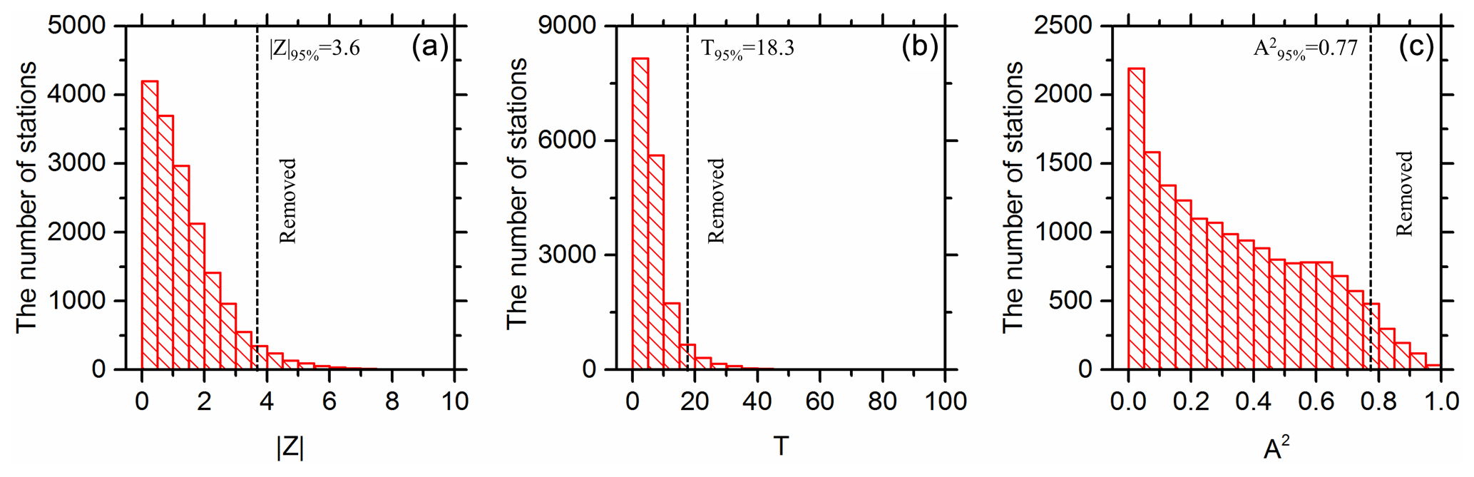
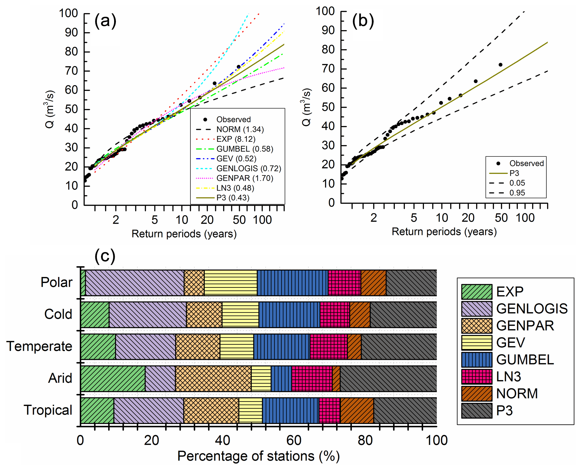
Figure 4Flood frequency curve selection and estimation. (a) Flood frequency curve selection of station no. AT0000032 (A2 value in brackets). (b) Design flood estimation of station no. AT0000032 using the Bayesian MCMC interface. (c) Selection results of flood frequency curve for all stations.
4.2 Subgroup delineation
For subgroup delineation, the number of clusters (K) and the clustering factors are two sensitive parameters. The value of K is selected by considering both the heterogeneity (reflected by the DB index) and the number of stations in the subgroup. Figure 5 describes the selection process of K when using all factors for clustering. As shown in Fig. 5a, the DB index reached an optimal value at K= 16 and then fluctuated with the increase of K. From Fig. 5b, we found that the number of stations in subgroups reduced with a larger K. To ensure a sufficient number of stations for model development for each subgroup, K greater than 40 is not considered in this research.

Figure 5Optimal K selection by (a) DB index and (b) the number of stations in subgroups during delineation.
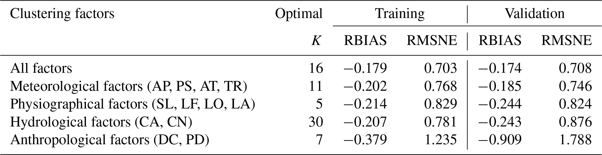
Taking the 100-year flood estimation as an example, different combinations of clustering factors were tested using the optimal K. As shown in Table 3, the best combination is to use all factors for clustering, and this result reaches the best RMSNE of 0.708 and RBIAS of −0.174 among all combinations for the validation periods. The design flood still could be satisfactorily estimated (RBIAS < 25 %) when using meteorological, physiographical or hydrological factors for clustering, respectively. Anthropological factors alone are not recommended for clustering as this results in the worst RMSNE of 1.788 and RBIAS of −0.909 among all combinations.
Table 3The impact of clustering factors on regional 100-year flood estimation.
4.3 Regression model comparison
Three regression models, PF, SVM and RF, were compared for 100-year flood estimation. Figure 6 describes the accuracy of the three models during training and validation periods. We found that PF showed the worse accuracy, with an RMSNE of 1.175 and 1.1089 in training and validation periods respectively. This reveals the coefficients of PF cannot accurately describe the contribution of factors to the results. RF gave the highest fitting ability during the training period, with an RMSNE of 0.290 and RBIAS of −0.037. However, the SVM model slightly outperformed the RF model during the validation period, with an RMSNE of 0.708 and RBIAS of −0.174. Therefore, SVM was selected for flood estimation for ungauged areas in this research.
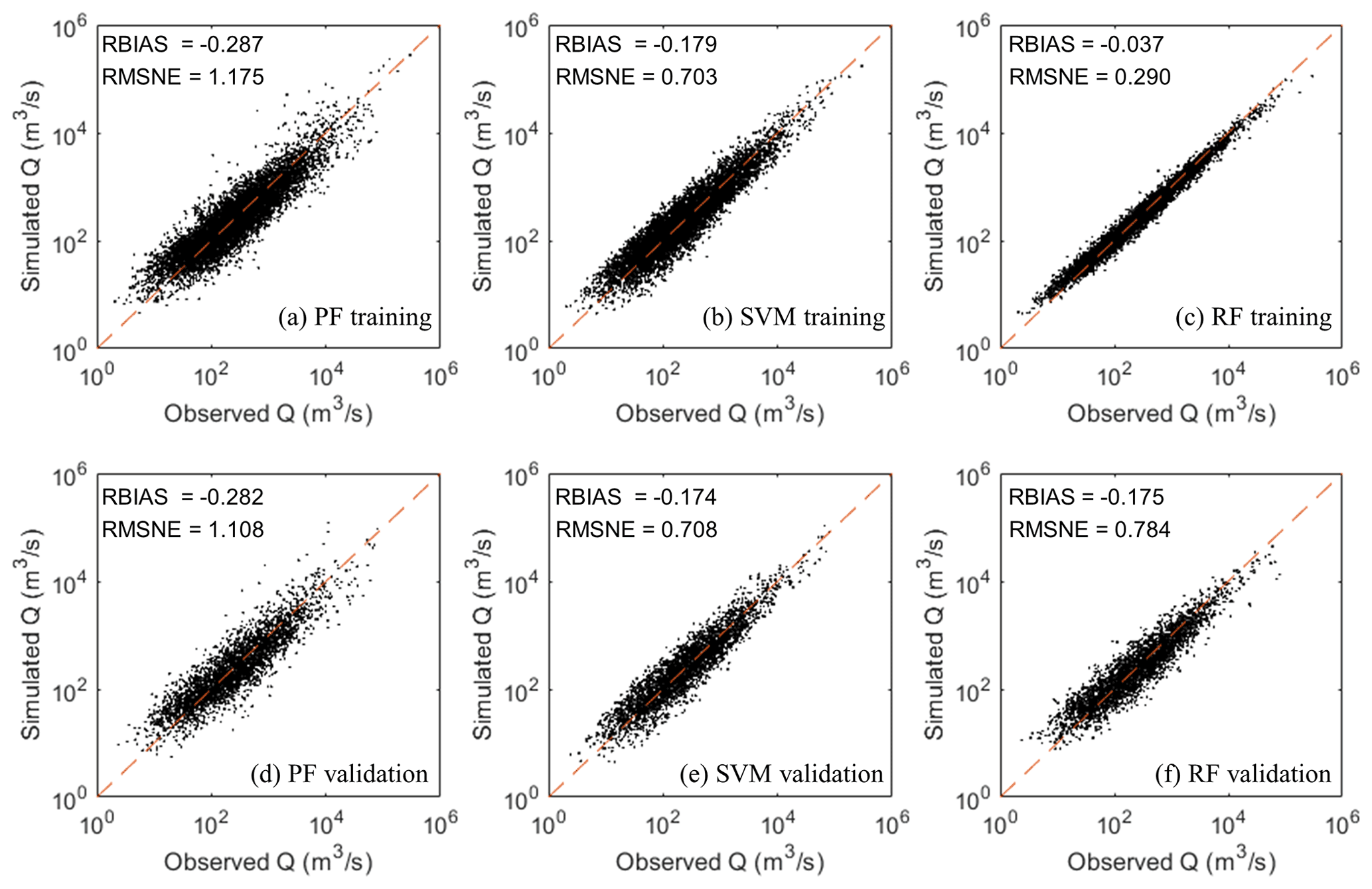
Figure 6Comparison of three regression models (PF, SVM and RF) during training and validation periods.
The factor importance in each subgroup was evaluated using the RF model, and Fig. 7a describes the range and average value of factor importance of all subgroups. The top four important factors are the catchment area (CA), annual precipitation (AP), longitude (LO) and latitude (LA). Meanwhile, dam capacity (DC) and curve number (CN) are the two least important factors and make up a relatively low proportion (average importance < 5 %) of the total importance among all factors.
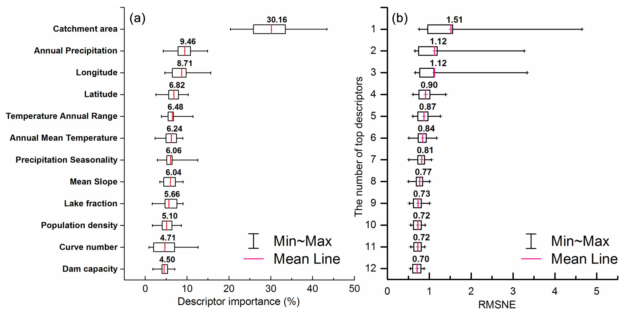
Figure 7(a) Descriptor importance evaluated by the RF model and (b) the optimal number of catchment descriptors for SVM regression.
To reduce model complexity, the type of descriptors for all subgroups was the same during training and validation. The optimal number of catchment descriptors used in the regression results was further tested based on the SVM regression and the factor importance order identified by the RF model. Figure 7b described the RMSNE for all subgroups during the validation period considering different combinations of catchment descriptors. AP and CA are the two most important factors and were also recommended as the catchment descriptors in the global RFFA approach of Smith et al. (2015), with a small number of samples (242 stations) for validation. When only using the CA and AP (top two factors) for regression and a large number of stations (3485 stations) for validation, the design flood cannot be accurately estimated (RMSNE > 1.0) for some subgroups. As shown in Fig. 7b, the prediction accuracy can be improved by considering more importance factors for model training and validation. After considering the top 10 factors for regression, the RMSNE of subgroups becomes stable and does not significantly improve by adding the further factors DC and CN. The SVM showed the highest performance considering all factors for regression (mean RMSNE of 0.70 in the validation period).
4.4 Regional flood estimation
Figure 8a–e demonstrate the simulated results from the optimal SVM model in each climate zone, and Fig. 8f displays the cumulative distribution function (CDF) between the simulated and observed discharge for all stations. Specially, the RMSNEs found were 0.746, 0.785, 0.722, 0.704 and 0.480 for tropical, arid, temperate, cold and polar climates respectively. Although there were some large individual errors, the SVM model showed good performance in tropical, temperature, cold and polar climate zones, with an RBIAS of −0.199, −0.169, −0.179 and −0.091 respectively. The SVM model showed a higher error of flood estimation in arid zones, with an RBIAS of −0.233. As shown in Fig. 8f, the simulated result can successfully fit the observed discharge curve given its likely error.
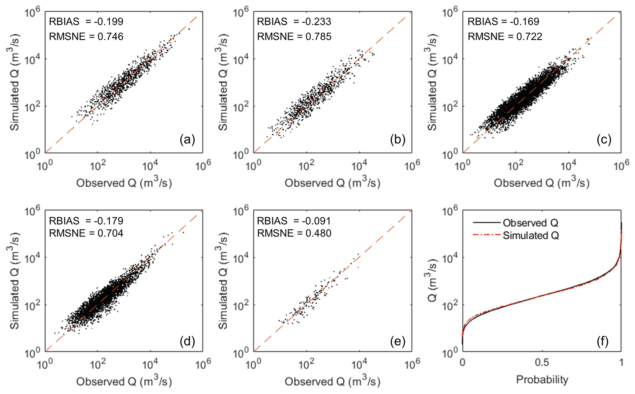
Figure 8Results of simulated Q100 in different climate zones, (a) tropical, (b) arid, (c) temperate, (d) cold and (e) polar. (f) Cumulative distribution function of simulated and observed discharge.
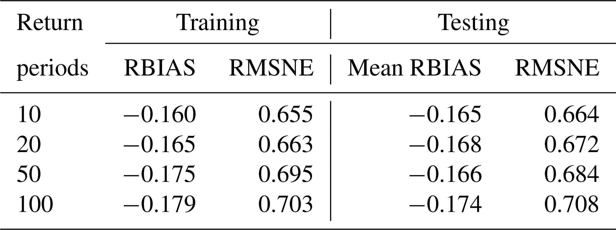
Table 4 compares the training and validation results of 10-, 20-, 50- and 100-year return period floods derived by the proposed direct regression method. By using the proposed direct regression method, all design floods could be estimated within the RBIAS of 0.18 (18 %). We found, unsurprisingly, that the prediction accuracy decreases with a larger flood magnitude. This is mainly because the at-site design flood is derived by observed data based on several assumptions, not the truth, and large return period floods are more difficult to be reliably estimated with limited observed data (Gaume, 2018). Regarding the natural and epistemic uncertainties in flood frequency analysis, the RBIAS of at-site design flood estimation was reported to be as large as 30 % in some studies (Di Baldassarre et al., 2012; Di Baldassarre and Montanari, 2009; Halbert et al., 2016; Merz and Thieken, 2005). As the at-site design flood is regarded as a training target, this error will be introduced in the regression and will directly affect the approach accuracy. Therefore, an RBIAS of 20 % or less is very impressive considering the uncertainties of at-site design flood estimation.
4.5 Discussion
In this research, we adopted a simple hold-out validation strategy such that 70 % and 30 % of stations were randomly selected for training and validation, respectively. To test the influence of hold-out samples on the model results, a 10-fold cross-validation strategy (Garmdareh et al., 2018; Lee et al., 2020) was applied. All stations in one subgroup were randomly divided into 10 folds. For every fold i (i= 1, 2, …, 10), the modeli was trained by the remaining 9 folds (except the ith fold) and validated by the ith fold. Using this strategy, 10 models were developed for each subgroup, and each sample in the original dataset was used for validation once. Table 5 describes the best, worse and median model performances validated by the different folds. We found that the selection of hold-out samples had a moderate impact on the PF model, and the RMSNE performance ranged from 0.97 to 1.49. Both SVM and RF showed more stable performances than PF, and SVM provided the narrowest range. We suggest using ensemble results from SVM models trained by different split samples to reduce the errors in sample selection.
Table 5Results of 100-year design flood estimation using 10-fold cross-validation.

We compared the flood estimation accuracy in different catchment sizes (Fig. 9a). Both over- and underestimations were found from small to large catchments. The range of RBIAS in small catchments is wider than that in large catchments. This reveals that design floods in small catchments are more difficult to estimate than large catchments. This is mainly because the catchment descriptors derived from global satellite images can have large uncertainties (McCabe et al., 2017) when describing small catchments and can lead to more substantial errors at low discharge. The negative value of RBIAS reflected some overestimation. Some studies suggested that the trends in observed discharge can lead to overestimation (or underestimation) of flood quantiles if such non-stationarity is not taken into consideration in RFFA (Kalai et al., 2020; O'Brien and Burn, 2014). Before model development, some non-stationary or discordant stations were eliminated from the whole dataset using a threshold of 5 %. This threshold is an empirical value and may remove some reliable stations if the sample is homogeneous. Figure 9b presents the model performances of training, testing and eliminated stations. We found that the proposed approach showed stable performance in the training and testing stations. However, the wide range of RBIAS in eliminated stations reveals that there may be some downsides in applying the proposed approach to a station where flows are changing rapidly. To address this limitation, the non-stationary RFFA approach should be explored in further research.
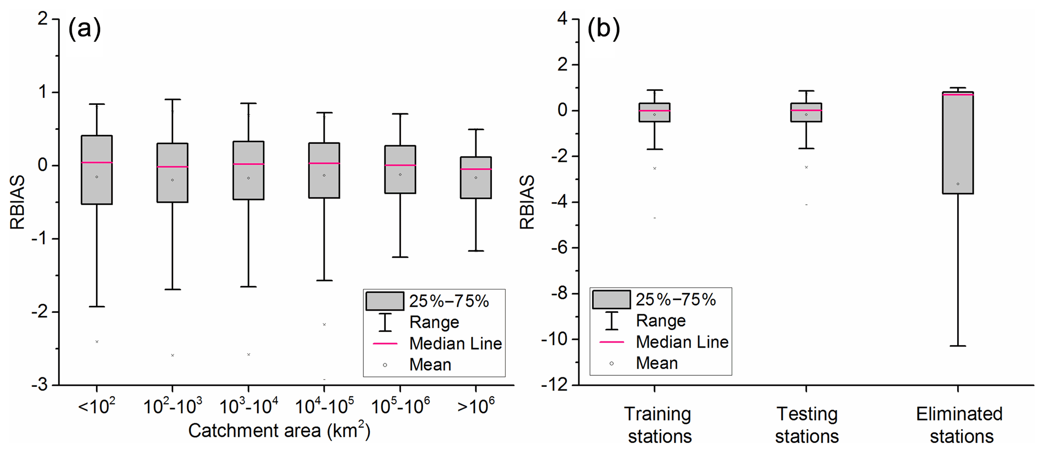
Figure 9RBIAS of 100-year return period flood estimation (a) in different catchment sizes and (b) in training, testing and eliminated stations.
All the proposed methods have not been implemented in a totally optimised way, the SVM model being slightly favoured in terms of the selected stations, not the whole initial GSIM dataset. Although only one-third of GSIM stations were selected, this research significantly improved the station density and model accuracy in all climate zones compared with the global RFFA of Smith (2015). The proposed approach achieved similar performances to some regional studies by adopting a global coverage of stations (Shu and Ouarda, 2008; Salinas et al., 2013). However, there can still be large errors in design flood estimation, especially in arid zones. This is consistent with previous research and is likely to be a result of drier regions being more heterogeneous (Salinas et al., 2013; Smith et al., 2015). In this study, the subgroups are delineated based on a widely used K-means model using squared Euclidean distance. Some studies showed that this model is not recommended for solving highly non-linear problems (Bárdossy et al., 2005; Samaniego et al., 2008; Raykov et al., 2016), and this may make it difficult to properly reflect the heterogeneous characteristics of the study area. Other clustering models and distance metrics that can better describe the non-linear relationship between descriptors should be compared in future studies.
A three-phase machine-learning-model-based approach was proposed to estimate design floods along river networks at the global scale. The at-site floods for global gauging station data were estimated based on a Bayesian MCMC method. The global stations were then clustered into several subgroups using a K-means clustering model, and a SVM regression was developed in each subarea for design flood estimation. Three widely used regression techniques, power-form function (PF), support vector machine (SVM) and random forests (RF), were compared for regression in each subgroup. The regional floods were final estimated using the same descriptors and the optimal SVM regression model.
The main conclusions of this study are summarised below:
-
To make reliable estimates, 11793 stations from the GSIM archive were selected for model implementation using stationarity, discordancy and homogeneity measures. For clustering, the impact of clustering number and clustering factors on estimation accuracy was tested. The best clustering number (K) was 16, which gave the lowest RMSNE of 0.708 for 100-year flood estimation when using all factors for clustering in a K-means model.
-
Three regression models were compared for 100-year flood estimation, and the SVM method showed the highest accuracy during the validation period, with an RMSNE of 0.708 and RBIAS of −0.174. Factor importance was identified using the RF model, and different combinations of factors were tested for the optimal SVM regression implementation. When only using the top two factors (annual precipitation and catchment area) for regression and a large number of stations (3485 stations) for validation, the design flood cannot be accurately estimated (RMSNE > 1.0) for some subgroups. After considering the top 10 factors for regression, the RMSNE for subgroups became stable and did not significantly improve by further adding factors.
-
The proposed approach showed good performance (i.e. the bias < ±20 %) in tropical, temperate, cold and polar climate zones, with an RBIAS of −0.199, −0.169, −0.179 and −0.091 respectively. A satisfying performance was found in arid areas with an RBIAS of −0.233. The negative value of RBIAS reflected some overestimation in RFFA.
This approach shows considerable promise for the estimation of extreme flood magnitudes at global scales, and the average RBIAS in estimation is less than 18 % for all design floods. This is likely to yield a significant improvement in the skill of global flood inundation models.
For a discharge series , the process of MKT is described in Eqs. (A1) to (A4):
The variance of S is computed as follows:
where n is the total number of time series Yi; Var(s) is the variance of S; and ti is the number of data points contained in the ith tie group.
The MKT statistic Z is given by
For a discharge series , the SNHT is described in Eqs. (B1) to (B4).
The SNHT statistic T is given by
where n is the total number of time series Yi; and and δ are the mean and standard deviation of time series Yi.
The Z score (ZS) method is described in Eq. (C1).
where Ri is the mean annual runoff of station i in one subgroup; is the mean value of Ri in one subgroup; and sd(R) is the standard deviation of Ri in one subgroup.
The L-moment-based method is presented in Eqs. (C2) to (C4).
where Nk is the number of stations in cluster k, and is the vector of the coefficient of L variation (L CV), L skewness and L kurtosis of the station i as defined by Hosking and Wallis (2005).
Table D1Hypothetical distributions adopted in this research.
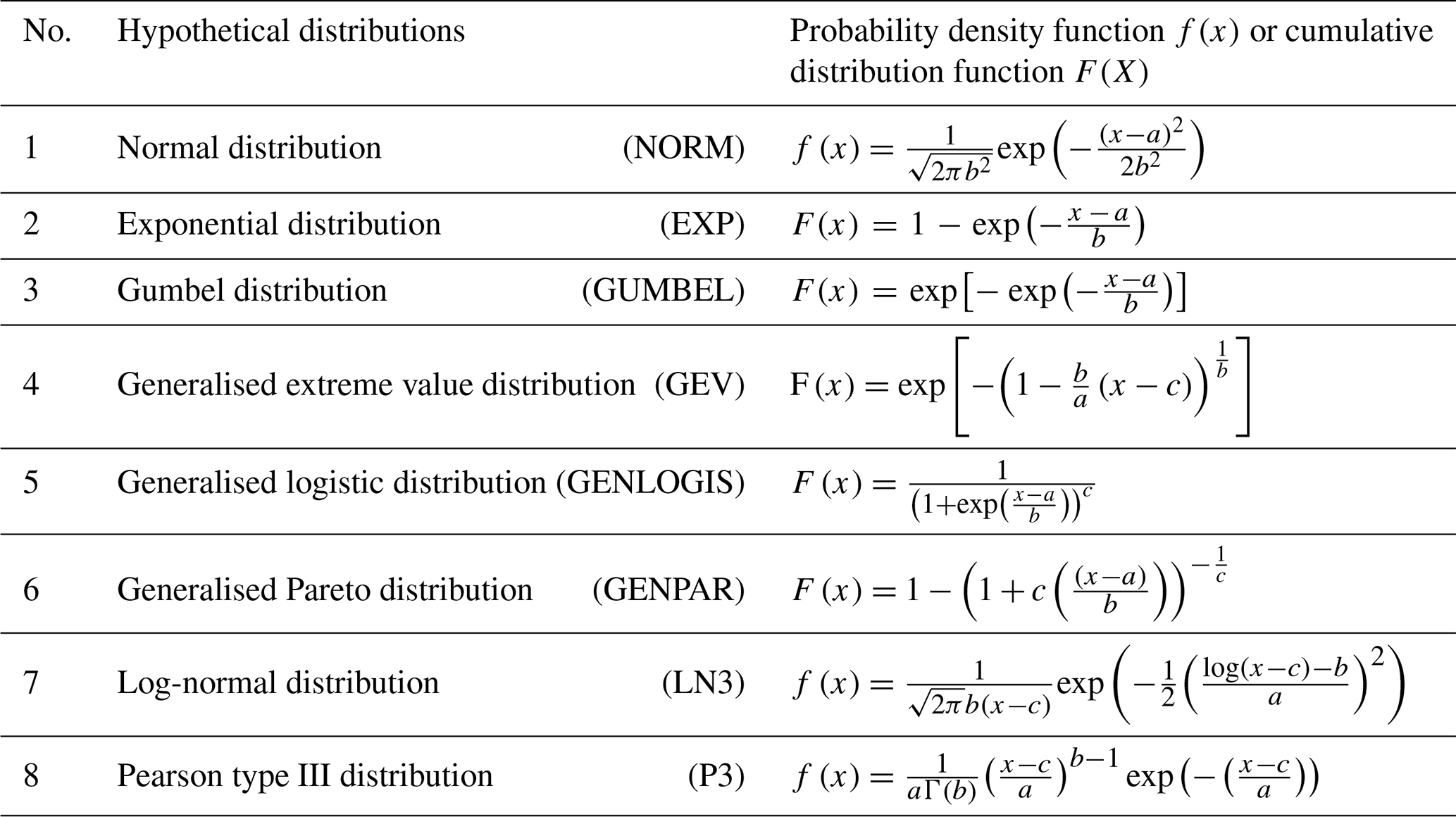
Note that x is the random variable; a, b and c are parameters of distributions.
Given a sample of data xi(i= 1, 2, …, m), the AD test will determine if a given dataset comes from a candidate cumulative distribution function F(x,θ) as in Eq. (E1), where θ is the parameter estimated by the sample xi.
where Fm(x) is the empirical cumulative distribution function; x(i) is the ith element of the sample in increasing order; and the AD test statistic A2 can be calculated as in Eq. (E2) (Ahmad et al., 1988; Laio, 2004).
The MKT and SNHT were implemented using the “trend” package (https://cran.r-project.org/web/packages/trend/index.html, Pohlert, 2021). The discordancy and at-site design floods were estimated based on the nsRFA package (https://CRAN.R-project.org/package=nsRFA, Viglione, 2021). The K-means, SVM and RF models are available from https://www.mathworks.com/help/stats/kmeans.html (MathWorks, 2021a), https://uk.mathworks.com/help/stats/support-vector-machine-regression.html (MathWorks, 2021b) and https://www.stat.berkeley.edu/~breiman/RandomForests/ (Breiman and Cutler, 2021) respectively.
The Global Streamflow Indices and Metadata Archive (GSIM) is freely available at https://doi.org/10.1594/PANGAEA.887477 (Do et al., 2018b). To access WorldClim – Global Climate Data, visit http://www.worldclim.org/ (Fick and Hijmans, 2021). The adopted terrain data are the MERIT-DEM at http://hydro.iis.u-tokyo.ac.jp/~yamadai/MERIT_DEM/ (Yamazaki, 2021). The Gridded Population of the World (GPW) dataset is available from https://sedac.ciesin.columbia.edu/data/collection/gpw-v4 (CIESIN, 2021). The Global Lakes and Wetlands Database (GLWD) is available from https://www.worldwildlife.org/pages/global-lakes-and-wetlands-database (Lehner and Döll, 2021). The data sources of the NRCS curve number dataset are described at https://doi.org/10.1080/2150704X.2017.1297544 (Zeng et al., 2017). The Global Reservoir and Dam Database (GRanD) can be downloaded by visiting http://globaldamwatch.org/grand/ (Beames et al., 2021).
GZ designed and conducted all experiments and analysed results under supervision from PB, JN and BP. All authors discussed and assisted with interpretation of the results and contributed to the article.
The authors declare that they have no conflict of interest.
Publisher's note: Copernicus Publications remains neutral with regard to jurisdictional claims in published maps and institutional affiliations.
Gang Zhao would like to thank Andrew Smith at Fathom for helpful discussions. We also thank the three reviewers and Luis Samaniego for their helpful review comments, which significantly improved the paper.
Paul Bates is supported by a Royal Society Wolfson Research Merit award. Jeff Neal is supported by NERC grants (grant nos. NE/S003061/1 and NE/S006079/1). Gang Zhao is supported by the China Scholarship Council–University of Bristol Joint PhD Scholarships Programme (grant no. 201700260088). Bo Pang is supported by the National Natural Science Foundation of China (grant no. 51879008).
This paper was edited by Luis Samaniego and reviewed by Eric Gaume, Dongyue Li, and one anonymous referee.
Ahmad, M. I., Sinclair, C., and Spurr, B.: Assessment of flood frequency models using empirical distribution function statistics, Water Resour. Res., 24, 1323–1328, 1988.
Alexandersson, H.: A Homogeneity Test Applied to Precipitation Data, J Climatol., 6, 661–675, https://doi.org/10.1002/joc.3370060607, 1986.
Bárdossy, A., Pegram, G. G., and Samaniego, L.: Modeling data relationships with a local variance reducing technique: Applications in hydrology, Water Resour. Res., 41, W08404, https://doi.org/10.1029/2004WR003851, 2005.
Bates, P. D., Quinn, N., Sampson, C., Smith, A., Wing, O., Sosa, J., Savage, J., Olcese, G., Neal, J., and Schumann, G.: Combined modelling of US fluvial, pluvial and coastal flood hazard under current and future climates, Water Resour. Res., e2020WR028673, https://doi.org/10.1029/2020WR028673, 2020.
Beames, P., Lehner, B., and Anand, M.: Global Reservoir and Dam Database (GRanD), available at: http://globaldamwatch.org/grand/, last access: October 2021.
Bocchiola, D., De Michele, C., and Rosso, R.: Review of recent advances in index flood estimation, Hydrol. Earth Syst. Sci., 7, 283–296, https://doi.org/10.5194/hess-7-283-2003, 2003.
Breiman, L. and Cutler, A.: Random Forests, available at: https://www.stat.berkeley.edu/~breiman/RandomForests/cc_home.htm, last access: October 2021.
Center for International Earth Science Information Network (CIESIN): Gridded Population of the World (GPW), v4, available at: https://sedac.ciesin.columbia.edu/data/collection/gpw-v4, last access: October 2021.
Chib, S. and Greenberg, E.: Understanding the metropolis-hastings algorithm, Am. Stat., 49, 327–335, 1995.
CRED and UNISDR: The Human Cost of Weather Related Disasters – 1995–2015, United Nations Office for Disaster Risk Reduction (UNISDR) and Centre for Research on the Epidemiology of Disasters (CRED), 2015.
Cunnane, C.: Methods and Merits of Regional Flood Frequency-Analysis, J. Hydrol., 100, 269–290, https://doi.org/10.1016/0022-1694(88)90188-6, 1988.
Dalrymple, T.: Flood-frequency analyses, manual of hydrology: Part 3, USGPO, https://doi.org/10.3133/wsp1543A, 1960.
Davies, D. L. and Bouldin, D. W.: A Cluster Separation Measure, IEEE T. Pattern Anal., PAMI-1, 224–227, https://doi.org/10.1109/TPAMI.1979.4766909, 1979.
Desai, S. and Ouarda, T. B.: Regional hydrological frequency analysis at ungauged sites with random forest regression, J. Hydrol., 594, 125861, https://doi.org/10.1016/j.jhydrol.2020.125861, 2021.
Di Baldassarre, G. and Montanari, A.: Uncertainty in river discharge observations: a quantitative analysis, Hydrol. Earth Syst. Sci., 13, 913–921, https://doi.org/10.5194/hess-13-913-2009, 2009.
Di Baldassarre, G., Laio, F., and Montanari, A.: Effect of observation errors on the uncertainty of design floods, Phys. Chem. Earth, Parts A/B/C, 42, 85–90, 2012.
Do, H. X., Gudmundsson, L., Leonard, M., and Westra, S.: The Global Streamflow Indices and Metadata Archive (GSIM) – Part 1: The production of a daily streamflow archive and metadata, Earth Syst. Sci. Data, 10, 765–785, https://doi.org/10.5194/essd-10-765-2018, 2018a.
Do, H. X., Gudmundsson, L., Leonard, M., and Westra, S.: Global Streamflow Indices and Metadata Archive – Part 1: Station catalog and Catchment boundary, PANGAEA, https://doi.org/10.1594/PANGAEA.887477, 2018b.
Doxsey-Whitfield, E., MacManus, K., Adamo, S. B., Pistolesi, L., Squires, J., Borkovska, O., and Baptista, S. R.: Taking advantage of the improved availability of census data: a first look at the gridded population of the world, version 4, Papers in Applied Geography, 1, 226–234, 2015.
Drucker, H., Burges, C. J., Kaufman, L., Smola, A., and Vapnik, V.: Support vector regression machines, Adv. Neural Inf. Process. Syst 9, 155–161, 1997.
Fick, S. E., and Hijmans, R. J.: WorldClim 2: new 1-km spatial resolution climate surfaces for global land areas, Int. J. Climatol., 37, 4302–4315, https://doi.org/10.1002/joc.5086, 2017.
Fick, S. E. and Hijmans, R. J.: Global climate and weather data, available at: https://worldclim.org/, last access: October 2021.
Frieler, K., Lange, S., Piontek, F., Reyer, C. P. O., Schewe, J., Warszawski, L., Zhao, F., Chini, L., Denvil, S., Emanuel, K., Geiger, T., Halladay, K., Hurtt, G., Mengel, M., Murakami, D., Ostberg, S., Popp, A., Riva, R., Stevanovic, M., Suzuki, T., Volkholz, J., Burke, E., Ciais, P., Ebi, K., Eddy, T. D., Elliott, J., Galbraith, E., Gosling, S. N., Hattermann, F., Hickler, T., Hinkel, J., Hof, C., Huber, V., Jägermeyr, J., Krysanova, V., Marcé, R., Müller Schmied, H., Mouratiadou, I., Pierson, D., Tittensor, D. P., Vautard, R., van Vliet, M., Biber, M. F., Betts, R. A., Bodirsky, B. L., Deryng, D., Frolking, S., Jones, C. D., Lotze, H. K., Lotze-Campen, H., Sahajpal, R., Thonicke, K., Tian, H., and Yamagata, Y.: Assessing the impacts of 1.5 ∘C global warming – simulation protocol of the Inter-Sectoral Impact Model Intercomparison Project (ISIMIP2b), Geosci. Model Dev., 10, 4321–4345, https://doi.org/10.5194/gmd-10-4321-2017, 2017.
Gao, S., Liu, P., Pan, Z., Ming, B., Guo, S., Cheng, L., and Wang, J.: Incorporating reservoir impacts into flood frequency distribution functions, J. Hydrol., 568, 234–246, 2019.
Garcia, F. A. A.: Tests to identify outliers in data series, Pontifical Catholic University of Rio de Janeiro, Industrial Engineering Department, Rio de Janeiro, Brazil, 2012.
Garmdareh, E. S., Vafakhah, M., and Eslamian, S. S.: Regional flood frequency analysis using support vector regression in arid and semi-arid regions of Iran, Hydrolog. Sci. J., 63, 426–440, https://doi.org/10.1080/02626667.2018.1432056, 2018.
Gaume, E.: Flood frequency analysis: The Bayesian choice, Wiley Interdisciplinary Reviews: Water, 5, e1290, https://doi.org/10.1002/wat2.1290, 2018.
Gizaw, M. S. and Gan, T. Y.: Regional Flood Frequency Analysis using Support Vector Regression under historical and future climate, J. Hydrol., 538, 387–398, https://doi.org/10.1016/j.jhydrol.2016.04.041, 2016.
Griffis, V. W. and Stedinger, J. R.: Log-Pearson Type 3 distribution and its application in flood frequency analysis. I: Distribution characteristics, J. Hydrol. Eng., 12, 482–491, https://doi.org/10.1061/(Asce)1084-0699(2007)12:5(482), 2007.
Gudmundsson, L., Do, H. X., Leonard, M., and Westra, S.: The Global Streamflow Indices and Metadata Archive (GSIM) – Part 2: Quality control, time-series indices and homogeneity assessment, Earth Syst. Sci. Data, 10, 787–804, https://doi.org/10.5194/essd-10-787-2018, 2018.
Haddad, K. and Rahman, A.: Selection of the best fit flood frequency distribution and parameter estimation procedure: a case study for Tasmania in Australia, Stoch. Env. Res. Risk A., 25, 415–428, 2011.
Halbert, K., Nguyen, C. C., Payrastre, O., and Gaume, E.: Reducing uncertainty in flood frequency analyses: A comparison of local and regional approaches involving information on extreme historical floods, J. Hydrol., 541, 90–98, 2016.
Hamed, K. H.: Trend detection in hydrologic data: the Mann–Kendall trend test under the scaling hypothesis, 349, 350–363, 2008.
Hammond, M. J., Chen, A. S., Djordjevic, S., Butler, D., and Mark, O.: Urban flood impact assessment: A state-of-the-art review, Urban Water J., 12, 14–29, https://doi.org/10.1080/1573062x.2013.857421, 2015.
Hosking, J. R. M. and Wallis, J. R.: The Effect of Intersite Dependence on Regional Flood Frequency-Analysis, Water Resour. Res., 24, 588–600, https://doi.org/10.1029/WR024i004p00588, 1988.
Hosking, J. R. M. and Wallis, J. R.: Regional frequency analysis: an approach based on L-moments, Cambridge University Press, Cambridge, https://doi.org/10.1017/CBO9780511529443, 2005.
Hutengs, C. and Vohland, M.: Downscaling land surface temperatures at regional scales with random forest regression, Remote Sens. Environ., 178, 127–141, https://doi.org/10.1016/j.rse.2016.03.006, 2016.
Kalai, C., Mondal, A., Griffin, A., and Stewart, E.: Comparison of nonstationary regional flood frequency analysis techniques based on the index-flood approach, J. Hydrol. Eng., 25, 06020003, https://doi.org/10.1061/(ASCE)HE.1943-5584.0001939, 2020.
Laio, F.: Cramer–von Mises and Anderson-Darling goodness of fit tests for extreme value distributions with unknown parameters, Water Resour. Res., 40, W09308, https://doi.org/10.1029/2004WR003204, 2004.
Lee, J.-Y., Choi, C., Kang, D., Kim, B. S., and Kim, T.-W.: Estimating Design Floods at Ungauged Watersheds in South Korea Using Machine Learning Models, Water, 12, 3022, https://doi.org/10.3390/w12113022, 2020.
Lehner, B. and Döll, P.: Development and validation of a global database of lakes, reservoirs and wetlands, J. Hydrol., 296, 1–22, https://doi.org/10.1016/j.jhydrol.2004.03.028, 2004.
Lehner, B. and Döll, P.: Global Lakes and Wetlands Database: Lakes and Wetlands Grid, available at: https://www.worldwildlife.org/pages/global-lakes-and-wetlands-database, last access: October 2021.
Lehner, B., Liermann, C. R., Revenga, C., Vorosmarty, C., Fekete, B., Crouzet, P., Doll, P., Endejan, M., Frenken, K., Magome, J., Nilsson, C., Robertson, J. C., Rodel, R., Sindorf, N., and Wisser, D.: High-resolution mapping of the world's reservoirs and dams for sustainable river-flow management, Front. Ecol. Environ., 9, 494–502, https://doi.org/10.1890/100125, 2011.
Li, B., Yang, G. S., Wan, R. R., Dai, X., and Zhang, Y. H.: Comparison of random forests and other statistical methods for the prediction of lake water level: a case study of the Poyang Lake in China, Hydrol. Res., 47, 69–83, https://doi.org/10.2166/nh.2016.264, 2016.
Lin, G. F. and Chen, L. H.: Identification of homogeneous regions for regional frequency analysis using the self-organizing map, J. Hydrol., 324, 1–9, https://doi.org/10.1016/j.jhydrol.2005.09.009, 2006.
Liu, X., Liu, W., Yang, H., Tang, Q., Flörke, M., Masaki, Y., Müller Schmied, H., Ostberg, S., Pokhrel, Y., Satoh, Y., and Wada, Y.: Multimodel assessments of human and climate impacts on mean annual streamflow in China, Hydrol. Earth Syst. Sci., 23, 1245–1261, https://doi.org/10.5194/hess-23-1245-2019, 2019.
MathWorks: kmeans, available at: https://www.mathworks.com/help/stats/kmeans.html, last access: October 2021a.
MathWorks: Support Vector Machine Regression, available at: https://uk.mathworks.com/help/stats/support-vector-machine-regression.html, last access: October 2021b.
McCabe, M. F., Rodell, M., Alsdorf, D. E., Miralles, D. G., Uijlenhoet, R., Wagner, W., Lucieer, A., Houborg, R., Verhoest, N. E. C., Franz, T. E., Shi, J., Gao, H., and Wood, E. F.: The future of Earth observation in hydrology, Hydrol. Earth Syst. Sci., 21, 3879–3914, https://doi.org/10.5194/hess-21-3879-2017, 2017.
Merz, R. and Blöschl, G.: Flood frequency hydrology: 2. Combining data evidence, Water Resour. Res., 44, W08433, https://doi.org/10.1029/2007wr006745, 2008a.
Merz, R. and Blöschl, G.: Flood frequency hydrology: 1. Temporal, spatial, and causal expansion of information, Water Resour. Res., 44, W08432, https://doi.org/10.1029/2007wr006744, 2008b.
Merz, B. and Thieken, A. H.: Separating natural and epistemic uncertainty in flood frequency analysis, J. Hydrol., 309, 114–132, 2005.
Müller Schmied, H., Adam, L., Eisner, S., Fink, G., Flörke, M., Kim, H., Oki, T., Portmann, F. T., Reinecke, R., Riedel, C., Song, Q., Zhang, J., and Döll, P.: Variations of global and continental water balance components as impacted by climate forcing uncertainty and human water use, Hydrol. Earth Syst. Sci., 20, 2877–2898, https://doi.org/10.5194/hess-20-2877-2016, 2016.
O'Brien, N. L., and Burn, D. H.: A nonstationary index-flood technique for estimating extreme quantiles for annual maximum streamflow, J. Hydrol., 519, 2040–2048, 2014.
Pohlert, T.: Non-Parametric Trend Tests and Change-Point Detection, available at: https://cran.r-project.org/web/packages/trend/index.html, last access: 31 October 2021.
Prihodko, L., Denning, A. S., Hanan, N. P., Baker, I., and Davis, K.: Sensitivity, uncertainty and time dependence of parameters in a complex land surface model, Agr. Forest Meteorol., 148, 268–287, https://doi.org/10.1016/j.agrformet.2007.08.006, 2008.
Raykov, Y. P., Boukouvalas, A., Baig, F., and Little, M. A.: What to do when K-means clustering fails: a simple yet principled alternative algorithm, PloS one, 11, e0162259, https://doi.org/10.1371/journal.pone.0162259, 2016.
Reis, D. S. and Stedinger, J. R.: Bayesian MCMC flood frequency analysis with historical information, J. Hydrol., 313, 97–116, 2005.
Richter, B. D., Baumgartner, J. V., Wigington, R., and Braun, D. P.: How much water does a river need?, Freshwater Biol, 37, 231–249, https://doi.org/10.1046/j.1365-2427.1997.00153.x, 1997.
Salinas, J. L., Laaha, G., Rogger, M., Parajka, J., Viglione, A., Sivapalan, M., and Blöschl, G.: Comparative assessment of predictions in ungauged basins – Part 2: Flood and low flow studies, Hydrol. Earth Syst. Sci., 17, 2637–2652, https://doi.org/10.5194/hess-17-2637-2013, 2013.
Samaniego, L., Bárdossy, A., and Schulz, K.: Supervised classification of remotely sensed imagery using a modified $ k $-NN technique, IEEE T. Geosci. Remote, 46, 2112–2125, 2008.
Sampson, C. C., Smith, A. M., Bates, P. B., Neal, J. C., Alfieri, L., and Freer, J. E.: A high-resolution global flood hazard model, Water Resour. Res., 51, 7358–7381, https://doi.org/10.1002/2015wr016954, 2015.
Schumann, G., Bates, P. D., Apel, H., and Aronica, G. T.: Global flood hazard mapping, modeling, and forecasting: challenges and perspectives, Global Flood Hazard: Applications in Modeling, Mapping, and Forecasting, 239–244, https://doi.org/10.1002/9781119217886.ch14, 2018.
Schumann, G. J. P., Andreadis, K. M., and Bates, P. D.: Downscaling coarse grid hydrodynamic model simulations over large domains, J. Hydrol., 508, 289–298, 2014a.
Schumann, G. J.-P., Andreadis, K. M., and Bates, P. D.: Downscaling coarse grid hydrodynamic model simulations over large domains, J. Hydrol., 508, 289–298, https://doi.org/10.1016/j.jhydrol.2013.08.051, 2014b.
Sharifi Garmdareh, E., Vafakhah, M., and Eslamian, S. S.: Regional flood frequency analysis using support vector regression in arid and semi-arid regions of Iran, Hydrolog. Sci. J., 63, 426–440, 2018.
Sharma, A., Wasko, C., and Lettenmaier, D. P.: If precipitation extremes are increasing, why aren't floods?, Water Resour. Res., 54, 8545–8551, 2018.
Shiffler, R. E. J. T. A. S.: Maximum Z scores and outliers, Am. Stat., 42, 79–80, 1988.
Shu, C., and Ouarda, T. B. M. J.: Regional flood frequency analysis at ungauged sites using the adaptive neuro-fuzzy inference system, J. Hydrol., 349, 31–43, https://doi.org/10.1016/j.jhydrol.2007.10.050, 2008.
Smith, A., Sampson, C., and Bates, P.: Regional flood frequency analysis at the global scale, Water Resour. Res., 51, 539–553, https://doi.org/10.1002/2014wr015814, 2015.
Stedinger, J. R.: Estimating a regional flood frequency distribution, Water Resour. Res., 19, 503–510, 1983.
Stein, L., Pianosi, F., and Woods, R.: Event-based classification for global study of river flood generating processes, Hydrol. Process., 34, 1514–1529, https://doi.org/10.1002/hyp.13678, 2019.
Teng, J., Jakeman, A. J., Vaze, J., Croke, B. F. W., Dutta, D., and Kim, S.: Flood inundation modelling: A review of methods, recent advances and uncertainty analysis, Environ. Modell. Softw., 90, 201–216, https://doi.org/10.1016/j.envsoft.2017.01.006, 2017.
Trigg, M. A., Birch, C. E., Neal, J. C., Bates, P. D., Smith, A., Sampson, C. C., Yamazaki, D., Hirabayashi, Y., Pappenberger, F., Dutra, E., Ward, P. J., Winsemius, H. C., Salamon, P., Dottori, F., Rudari, R., Kappes, M. S., Simpson, A. L., Hadzilacos, G., and Fewtrell, T. J.: The credibility challenge for global fluvial flood risk analysis, Environ. Res. Lett., 11, 094014, https://doi.org/10.1088/1748-9326/11/9/094014, 2016.
United States Soil Conservation Service: National Engineering Handbook, Section 19, Construction Inspection, Washington, D.C., U.S. Dept. of Agriculture, Soil Conservation Service, 1985.
Viglione, A.: Non-Supervised Regional Frequency Analysis, available at: https://CRAN.R-project.org/package=nsRFA, last access: October 2021.
Vogel, R. M., McMahon, T. A., and Chiew, F. H.: Floodflow frequency model selection in Australia, J. Hydrol., 146, 421–449, 1993.
Wang, J., Liang, Z., Hu, Y., and Wang, D.: Modified weighted function method with the incorporation of historical floods into systematic sample for parameter estimation of Pearson type three distribution, J. Hydrol., 527, 958–966, 2015.
Water Resources Council (US): Hydrology Committee, Guidelines for determining flood flow frequency, US Water Resources Council, Hydrology Committee, 1975.
Wing, O. E., Bates, P. D., Sampson, C. C., Smith, A. M., Johnson, K. A., and Erickson, T. A. J. W. R. R.: Validation of a 30 m resolution flood hazard model of the conterminous United States, Water Resour. Res., 53, 7968–7986, 2017.
Wing, O. E., Bates, P. D., Smith, A. M., Sampson, C. C., Johnson, K. A., Fargione, J., and Morefield, P.: Estimates of present and future flood risk in the conterminous United States, Environ. Res. Lett., 13, 034023, https://doi.org/10.1088/1748-9326/aaac65, 2018.
Winsemius, H. C., Van Beek, L. P. H., Jongman, B., Ward, P. J., and Bouwman, A.: A framework for global river flood risk assessments, Hydrol. Earth Syst. Sci., 17, 1871–1892, https://doi.org/10.5194/hess-17-1871-2013, 2013.
Winsemius, H. C., Aerts, J. C., Van Beek, L. P., Bierkens, M. F., Bouwman, A., Jongman, B., Kwadijk, J. C., Ligtvoet, W., Lucas, P. L., and Van Vuuren, D. P.: Global drivers of future river flood risk, Nat. Clim. Change, 6, 381–385, 2016.
Yamazaki, D., Kanae, S., Kim, H., and Oki, T.: A physically based description of floodplain inundation dynamics in a global river routing model, Water Resour. Res., 47, W04501, https://doi.org/10.1029/2010wr009726, 2011.
Yamazaki, D.: MERIT DEM: Multi-Error-Removed Improved-Terrain DEM, available at: http://hydro.iis.u-tokyo.ac.jp/~yamadai/MERIT_DEM/, last access: October 2021.
Yamazaki, D., Ikeshima, D., Tawatari, R., Yamaguchi, T., O'Loughlin, F., Neal, J. C., Sampson, C. C., Kanae, S., and Bates, P. D.: A high-accuracy map of global terrain elevations, Geophys. Res. Lett., 44, 5844–5853, https://doi.org/10.1002/2017gl072874, 2017.
Yang, T., Sun, F., Gentine, P., Liu, W., Wang, H., Yin, J., Du, M., and Changming, L.: Evaluation and machine learning improvement of global flood simulations, AGUFM, 2019, H33L-2122, 2019a.
Yang, T., Sun, F., Gentine, P., Liu, W., Wang, H., Yin, J., Du, M., and Liu, C.: Evaluation and machine learning improvement of global hydrological model-based flood simulations, Environ. Res. Lett., 14, 114027, https://doi.org/10.1088/1748-9326/ab4d5e, 2019b.
Zeng, Z. Y., Tang, G. Q., Hong, Y., Zeng, C., and Yang, Y.: Development of an NRCS curve number global dataset using the latest geospatial remote sensing data for worldwide hydrologic applications, Remote Sens. Lett., 8, 528–536, https://doi.org/10.1080/2150704x.2017.1297544, 2017.
Zhang, Y., Chiew, F. H., Li, M., and Post, D.: Predicting runoff signatures using regression and hydrological modeling approaches, Water Resour. Res., 54, 7859–7878, 2018.
Zhao, G., Pang, B., Xu, Z. X., Yue, J. J., and Tu, T. B.: Mapping flood susceptibility in mountainous areas on a national scale in China, Sci. Total Environ., 615, 1133–1142, https://doi.org/10.1016/j.scitotenv.2017.10.037, 2018.
Zhao, G., Bates, P., and Neal, J.: The impact of dams on design floods in the Conterminous US, Water Resour. Res., 56, e2019WR025380, https://doi.org/10.1029/2019WR025380, 2020.
- Abstract
- Introduction
- Study areas and data
- Methodology
- Results and discussion
- Conclusions
- Appendix A: Mann–Kendall test (MKT)
- Appendix B: Standard normal homogeneity test (SNHT)
- Appendix C: Discordancy measure methods
- Appendix D: Hypothetical distributions
- Appendix E: Anderson–Darling (AD) test
- Code availability
- Data availability
- Author contributions
- Competing interests
- Disclaimer
- Acknowledgements
- Financial support
- Review statement
- References