the Creative Commons Attribution 4.0 License.
the Creative Commons Attribution 4.0 License.
 | 15 Nov 2021
Rainfall-induced shallow landslides and soil wetness: comparison of physically based and probabilistic predictions
Elena Leonarduzzi
Brian W. McArdell
Peter Molnar
Landslides are an impacting natural hazard in alpine regions, calling for effective forecasting and warning systems. Here we compare two methods (physically based and probabilistic) for the prediction of shallow rainfall-induced landslides in an application to Switzerland, with a specific focus on the value of antecedent soil wetness. First, we show that landslide susceptibility predicted by the factor of safety in the infinite slope model is strongly dependent on soil data inputs, limiting the hydrologically active range where landslides can occur to only ∼20 % of the country with typical soil parameters and soil depth models, not accounting for uncertainty. Second, we find the soil saturation estimate provided by a conceptual hydrological model (PREVAH) to be more informative for landslide prediction than that estimated by the physically based coarse-resolution model (TerrSysMP), which we attribute to the lack of temporal variability and coarse spatial resolution in the latter. Nevertheless, combining the soil water state estimates in TerrSysMP with the infinite slope approach improves the separation between landslide triggering and non-triggering rainfall events. Third, we demonstrate the added value of antecedent soil saturation in combination with rainfall thresholds. We propose a sequential threshold approach, where events are first split into dry and wet antecedent conditions by an N d (day) antecedent soil saturation threshold, and then two different total rainfall–duration threshold curves are estimated. This, among all different approaches explored, is found to be the most successful for landslide prediction.
- Article
(10004 KB) - Full-text XML
- BibTeX
- EndNote


Landslides are a natural hazard affecting alpine regions worldwide. They damage infrastructure and buildings, sometimes leading to loss of life (e.g. Kjekstad and Highland, 2009; Salvati et al., 2010; Petley, 2012; Trezzini et al., 2013; Mirus et al., 2020). Shallow landslides occur when and where the applied shear on the soil–bedrock interface exceeds the shear strength of the soil on a slope. Their occurrence is determined by two key factors: predisposing factors, which are a collection of soil and land surface properties of a certain location which make it susceptible (or not) to landsliding (e.g. Reichenbach et al., 2018), and triggering factors, which are those that initiate slope failure on susceptible slopes. In general, most landslides are either triggered by earthquakes or rainfall (e.g. Iverson, 2000; Highland and Bobrowsky, 2008; Leonarduzzi et al., 2017; Marc et al., 2019). Here we focus on shallow rainfall-induced landslides, which involve the top layer of the soil, typically less than 2 m thick, and fail instantaneously. In such landslides, failure is typically the result of the development of positive pore water pressure in the soil, which decreases its strength (e.g. Anderson and Sitar, 1995; Highland and Bobrowsky, 2008). This condition is often associated with intense or long-lasting rainfall events that saturate the soil by vertical infiltration and lateral subsurface drainage. The wetness of the soil prior to the triggering rainfall is therefore a key ingredient in slope failure (Bogaard and Greco, 2018).
Several approaches exist for the prediction of landslides that focus on one or more predisposing and triggering factors, typically classified into three types: susceptibility mapping, probabilistic approaches, and physically based modelling (e.g. Aleotti and Chowdhury, 1999).
Susceptibility mapping assesses the vulnerability of a certain area to landsliding based on predisposing factors. In statistical susceptibility mapping, the different predisposing factors, geological, topographical, and climatological properties, are combined with landslide inventories and used as explanatory variables in a statistical model (e.g. Reichenbach et al., 2018). Landslide hazard maps are then generated by various forms of linear and non-linear multivariate regression models (e.g. Chung et al., 1995), logistic regression (e.g. Ohlmacher and Davis, 2003; Ayalew and Yamagishi, 2005; Lee and Pradhan, 2007; Yilmaz, 2009; von Ruette et al., 2011), or machine learning algorithms (e.g. Saito et al., 2009; Ermini et al., 2005; Yilmaz, 2009). Susceptibility mapping can also be achieved by applying a physically based geotechnical model which identifies the likelihood of failure in a region based on an assessment of likely soil water distribution in space (e.g. Baum et al., 2002, 2008; Dietrich and Montgomery, 1998; Formetta et al., 2016).
Probabilistic approaches focus mainly on the temporal component of the landslide hazard (triggering factors) rather than the spatial susceptibility (predisposing factors). They are based on the assumption that rainfall is the main triggering factor and take advantage of historical records of rainfall and landslides. These databases are combined to learn which meteorological conditions have been associated with the triggering of landslides in the past. This allows us then to recognise critical conditions in weather forecasts of the coming days and estimate how likely the occurrence of landsliding is. The most common of these approaches is that of rainfall thresholds, and in particular intensity–duration or total rainfall–duration threshold curves (e.g. Guzzetti et al., 2007; Leonarduzzi et al., 2017; Segoni et al., 2018). While rainfall is the main triggering factor, soil wetness conditions prior to triggering rainfall can also be included in this framework (e.g. Bogaard and Greco, 2018; Marino et al., 2020). The antecedent soil wetness conditions can be derived in many different ways, each with its advantages and limitations, e.g. from in situ measurements (depend on network density, e.g. Wicki et al., 2020), remote sensing of soil moisture (suffer from low resolution and insufficient penetrating depth, e.g. Brocca et al., 2012; Thomas et al., 2019), through proxies of soil wetness like antecedent rainfall (miss evapotranspiration and snowmelt, e.g. Glade et al., 2000; Godt et al., 2006; Mathew et al., 2014), or by hydrological soil water balance modelling (e.g. Ponziani et al., 2012; Thomas et al., 2018).
Finally, physically based modelling approaches are usually made up of two components to directly simulate slope stability in time and space: a hydrological and a geotechnical model. The hydrological model is used to estimate the condition of the soil, i.e. the pore water pressure and/or saturation, which are then used in the geotechnical model for the estimation of slope stability (e.g. by the infinite slope or other hydromechanical slope failure model). These approaches are theoretically the most sound and predict both when and where a landslide could occur, but they are computationally expensive and data demanding. For these reasons, they are typically applied on individual slopes in landslide-prone areas or small catchments only (Cohen et al., 2009; von Ruette et al., 2013; Anagnostopoulos et al., 2015; Fan et al., 2015, 2016).
In this work, we conduct a comparison of a probabilistic and physically based modelling approach to landslide prediction with the specific question of the value of the inclusion of antecedent soil wetness state in the prediction. Our scale of analysis is regional (Switzerland) instead of hillslope/catchment scale, because it is at this scale that landslide early warning systems need to be developed (e.g. Staehli et al., 2015). First we explore the regional susceptibility to landslides following the infinite slope approach (physically based susceptibility mapping). This allows us to understand where hydrology can play a role in the landscape in triggering landslides, i.e. identifying areas where the transient soil wetness results in the factor of safety (FoS) fluctuating above 1 (stable) and below 1 (unstable). We then explore two approaches to account for the soil wetness state for landslide prediction, taking advantage of the hydrological estimates of soil moisture provided by two different model set-ups for forecasting purposes and covering Switzerland.
-
A fully physically based approach that takes advantage of a state-of-the-art European simulation of hydrology (Furusho-Percot et al., 2019) with three physically based coupled models (climate forecast model, land surface model, hydrological model) at a coarse resolution (12.5 km × 12.5 km), from which we extract pore water pressure. The pressure field is then used as a dynamic component in the factor of safety estimation in the infinite slope approach. This framework is designed based on similar existing blueprints for landslide warning systems (Schmidt et al., 2008; Wang et al., 2020).
-
A probabilistic approach in which we develop rainfall threshold curves for landslide prediction based on a combination of historical databases of rainfall and landslides for Switzerland (Leonarduzzi et al., 2017). We then combine these predictions with estimated soil saturation by a Swiss operational, semi-distributed conceptual hydrological model (PREVAH; Viviroli et al., 2009) to quantify the strength of the signal in antecedent soil moisture which could be used in rainfall threshold curve methods for landslide prediction at this scale.
The comparison between the two approaches allows us to answer the following questions. (1) Is the infinite slope approach valuable for landslide hazard assessment at the regional scale? (2) Where does hydrology play a role in the triggering of landslides in Switzerland? (3) Which hydrological soil water estimate (PREVAH or TerrSysMP) is more informative for landslide prediction and why? (4) How can we best take advantage of the soil saturation estimates in combination with rainfall characteristics for landslide prediction?
2.1 Physically based approach
2.1.1 The infinite slope model
For the stability assessment, we choose to follow the infinite slope approach, because this is one of the most widely used models for slope failure prediction (e.g. Pack et al., 1998; Iverson, 2000; Baum et al., 2008; Lu and Godt, 2008). It is based on the assumption that the thickness of the sliding mass (soil) is much smaller than the length of the slope, which is typically true for shallow landslides (up to 2 m deep). The factor of safety (FoS) is computed as the ratio between soil shear strength and applied stress to the soil layer:
where h is the water pressure head within the soil layer [m] (see Sect. 2.1.3), d the soil depth [m] (see Sect. 2.1.2), c is soil cohesion [Pa], γ is soil unit weight [N/m2] (computed from the bulk soil density ρ and gravitational acceleration g as ), γw is the specific weight of water [N/m2], β is the slope angle [rad], and ϕ is the soil internal friction angle [rad]. Typically FoS = 1 is assumed to be the threshold of failure, with landsliding occurring when FoS < 1, i.e. when the applied shear stress exceeds the soil shear strength.
All calculations are done at the resolution of the DEM, i.e. a grid of cell size 25 m × 25 m in this paper. This resolution is a result of testing (not reported here) and a compromise between not violating the infinite slope assumptions (length scale of landslides ≫ their depth) and keeping the grid size similar to that of a typical landslide detachment area while also capturing local topographic gradients β, which are smoothed as resolution decreases.
To estimate the bulk soil density, cohesion, and friction angle, we used publicly available datasets in OpenLandMap (OpenLandMap, 2020; Hengl et al., 2017), which provide global maps of a wide range of soil, land cover, hydrology, geology, climate, and relief characteristics. All the maps used here are available at a resolution of approximately 250 m × 250 m. The soil properties are provided for six different depths up to 200 cm produced by machine learning algorithms trained on soil profiles globally (SoilGrids dataset). For the estimation of the bulk soil density, we compute the thickness-weighted average for the 2 m soil column. For the friction angle, we first associate a value for each soil texture class (USDA system) present in Switzerland in the OpenLandMap dataset (Geotechdata.info, Angle of Friction, 2013). Then at each location, we choose the value of the friction angle at the depth corresponding to the local soil depth (e.g. if the soil is 120 cm deep locally, the closest value in SoilGrids will be that at 1 m depth). Finally for cohesion, we assume that the soil itself is cohesionless (c=0), but we add the important contribution of vegetation to cohesion on slopes. From the land-cover map in OpenLandMap, we identify eight classes of tree cover, and we assign them a cohesion value between kPa. Denser tree cover and mixed forests are associated with larger values of cohesion (Schwarz et al., 2012; Dorren and Schwarz, 2016). To quantify the sensitivity of the FoS estimation to the apparent root cohesion, we also simulate the reference case in which cohesion is assumed c=0 over the entire country (Fig. 1). All maps are downscaled to 25 m × 25 m resolution by resampling with nearest neighbour.

Figure 1Maps of the distributed input used in the factor of safety calculations. (a) The 25 m digital elevation model (Swisstopo), (b) friction angle obtained from the OpenLandMap USDA texture class and provided soil depth, (c) bulk density obtained from OpenLandMap, and (d) cohesion estimated for the land-cover map from OpenLandMap. The friction angle depends on the local soil depth; here soil depth is estimated with the linear diffusion model.
To assess the susceptibility to landsliding in Switzerland, we compute the factor of safety of the two endmember scenarios: completely wet soil (h=d) or completely dry soil (h=0), which give us the minimum and maximum FoS. This allows us to identify unconditionally stable and unstable areas in our domain just based on hydrology and soil and topographic characteristics. Unconditionally stable areas have the minimum FoS > 1 for a completely wet soil and will never fail regardless of the actual hydrological state. Unconditionally unstable areas have the maximum FoS < 1 for a completely dry soil and will (should) always fail according to Eq. (1). In all other areas, hydrology plays a role in the initiation of landslides according to the FoS methodology.
We then compute the dynamic factor of safety in time and its statistics for all cells (25 m × 25 m) in which at least one landslide was recorded according to the landslide database (for details on the database see Sect. 2.2), using the water pressure head h estimated from the hydrological model described in Sect. 2.1.3. Additionally, we also compute the departure of the minimum FoS from the local temporal mean (i.e. mean of the 25 m cell) during each triggering and non-triggering rainfall event which are defined in Sect. 2.2. These analyses allow us to observe variations in FoS at cell level and relate them to observed landslide occurrence at those locations. If these relations are found to be strong, we hypothesise that a warning system could be based on the estimated FoS. Otherwise, its use for landslide warning is questionable.
2.1.2 Soil depth
Because soil depth is the most poorly known variable and uncertain parameter in the slope stability model in Eq. (1), here we use four different methods to estimate soil thickness distributions in space and test their impacts on FoS estimates. (1) Uniform soil depth of 1 m for the entire country is the first method. (2) The slope-dependent model is given as follows (Saulnier et al., 1997):
where dmax is maximum soil depth, dmin is the minimum soil depth (assumed to be 5 cm), βi is the local slope, βmax is the maximum slope above which no soil layer can form (assumed to be 45∘), and βmin is the minimum slope (0∘). (3) The elevation-dependent model is given as follows (Saulnier et al., 1997):
where zi is the local elevation, zmax is the maximum elevation, and zmin is the minimum elevation. (4) The steady-state soil depth produced by the linear diffusion transport model (Roering, 2008) is the fourth method where we simulate the distributed soil depth after 15 000 years of soil development. This approach is based on mass conservation (Eq. 4), with soil production decreasing exponentially with soil depth (Eq. 5), and soil erosion and transport assumed to be linearly dependent on slope (Eq. 6).
where is the change of soil depth in time, qs,i the soil (sediment) transport vector at location i, the ratio between the bedrock and soil density (2 as in Dietrich et al., 1995), ϵi the soil production rate at location i, ϵ0 the maximum soil production rate associated with 0 depth (0.000268 m per year as in Heimsath et al., 2001), β the slope angle at location i, μ the critical value depth (3/m as in Roering, 2008), Kl the coefficient of linear proportionality (0.0050 as in Dietrich et al., 1995), and ∇zi the gradient of elevation at location i.
For the soil depth models (2)–(4), we fix the maximum soil depth dmax=2 m to be consistent. In fact, no deeper soil depths are reported in the Swiss soil suitability map for agriculture (Bodeneignungskarte der Schweiz, 2020).
2.1.3 Hydrology
The water pressure head within the soil layer required for the calculation of the factor of safety (h in Eq. 1) is provided by an operational European forecasting system. This consists of the climatology from 1989 to current day, obtained by applying the Terrestrial Systems Modeling Platform (TerrSysMP) (Kurtz et al., 2016). This platform is made up of three physically based coupled models that solve the water and energy fluxes from the atmosphere to the groundwater: a weather prediction model, a land surface process model, and a hydrological model for surface and subsurface 3D water fluxes. TerrSysMP is produced at daily resolution over a 12.5 km × 12.5 km grid covering Europe. Several state and flux variables are available and can be freely accessed; here we use the water pressure in the soil and soil saturation.
We extract from the historical simulations the water pressure at the depth obtained by the soil depth model chosen and correct for the elevation difference between the centre of the corresponding TerrSysMP vertical layer and the estimated local depth and use it as the water pressure head term in Eq. (1), h. In addition to pressure, we also extract the average saturation of the top two soil layers (total depth of 60 cm from the surface), in order to facilitate comparisons with the saturation obtained by the conceptual hydrological model PREVAH.
2.2 Probabilistic approach
2.2.1 Rainfall threshold curves
We combine landslide inventory data in Switzerland and a daily gridded dataset of rainfall to develop rainfall threshold curves following the method by Leonarduzzi et al. (2017). The historical landslides were collected in the Swiss flood and landslide damage database (Swiss Federal Research Institute WSL; Hilker et al., 2009). This database contains floods, landslides, and rockfall events which produced damages in Switzerland since 1972. We select the landslide events that have a known location and date and were not associated with snowmelt, for a total of 1807 events between 1981 and 2016 (time frame of the analysis). The rainfall record is obtained as the interpolation of a network of ca. 430–460 rain gauges, using the local climatology and regional precipitation–topography relationships (Shepard, 1984; Frei and Schär, 1998; Frei et al., 2006). It contains daily rainfall totals on a 1 km × 1 km grid covering the entire country since 1961.
For the definition of rainfall events, we follow the procedure introduced in Leonarduzzi et al. (2017). First we select susceptible cells, i.e. rainfall cells (1 km × 1 km grid cells) where at least one landslide was recorded. For those cells, we separate the rainfall time series into events, where an event is defined as a series of consecutive rainy days with a minimum of 1 dry day between events. These events are then classified as observed triggering if a landslide was recorded during or immediately after them and non-triggering otherwise. The properties of each event are total rainfall depth (E), event duration (D), event mean daily intensity, and event maximum daily intensity.
We then define a power-law total rainfall–duration (ED) threshold curve E=aDb that separates triggering and non-triggering rainfall events. To this end, we estimate the a and b parameters of the power-law curve by maximising the true skill statistic (TSS = true positive ratio − false positive ratio), as in Leonarduzzi et al. (2017). This allows us to classify the rainfall events by the calibrated ED threshold into the following groups (see also Leonarduzzi and Molnar, 2020): observed and correctly predicted triggering events above the ED curve (true positive), observed triggering events which fall below the ED curve (false negative), observed non-triggering events which fall above the ED curve (false positive), and observed non-triggering events which fall below the ED curve (true negative).
2.2.2 Antecedent soil saturation
We use the values of soil saturation estimated by the Swiss operational hydrological model PREVAH (Viviroli et al., 2009) at a 500 m × 500 m resolution to explore the added value of antecedent soil saturation on the ED curve predictions. PREVAH is a conceptual model, where the soil is represented by three storage modules: soil moisture storage (SSM), upper zone (unsaturated) runoff storage (SUZ), and lower zone (saturated) runoff storage. We use the values of the first two (unsaturated) layers and combine and transform them into a 0–1 soil saturation estimate. This is computed as , where SUZmax is a distributed calibrated parameter, while SSMmax is the maximum value of SSM simulated over the entire time frame (1981–2018) at each grid cell.
For each susceptible cell defined in Sect. 2.2.1, we extract the time series of the PREVAH soil saturation estimate at the corresponding cell, and we compute the departure of the maximum saturation during triggering and non-triggering rainfall events from the local temporal mean and the N d mean antecedent saturation (N=1, 2, 5, 10, 20, 30, 60 d).
We test the information content of soil saturation for the ED curves, i.e. analyse whether information on soil saturation could reduce some of the false positives and negatives generated by the ED threshold curve estimated in Sect. 2.2.1. For each group of events (false positives, false negatives, true positives, and true negatives) and each rainfall event duration (1 to 6 d), we compute the mean soil saturation over 5–60 d prior to the beginning of the event. This allows us to examine if we fail to predict some triggering events (false negative) with the ED curve because saturation was very high, reducing the rainfall amount required for the initiation of a landslide, and likewise if some larger rainfall amounts were insufficient for the triggering (false positive) because the soil was very dry prior to rainfall.
Finally we explore two different approaches to combine rainfall characteristics and antecedent saturation. On the one hand, a hydrometeorological threshold separating the antecedent N d mean saturation (with N=1, 2, 5, 10, 20, 30, 60 d) and rainfall characteristic (logarithm of either total rainfall, maximum or mean intensity) pairs for triggering and non-triggering events. On the other hand, a sequential threshold system where events are first split into high and low N d antecedent saturation, and then two different ED thresholds are used accordingly, for wet and dry antecedent conditions (e.g. Sidle and Ochiai, 2006). We optimise the saturation and ED thresholds by maximising the TSS, but we also consider different antecedent saturation periods (N=1, 2, 5, 10, 20, 30, 60 d). We propose that such thresholds could be used in a landslide warning context together with estimated current soil wetness and forecasted rainfall.
3.1 Physically based approach
3.1.1 Infinite slope model spatial patterns
Distributed inputs (Fig. 1) are used to compute the FoS across Switzerland as a function of the hydrological term h for the two endmember states h=0 and h=d. As a first step, we generate the distributed soil depth values following the four approaches introduced in Sect. 2.1.2 (Fig. 2).
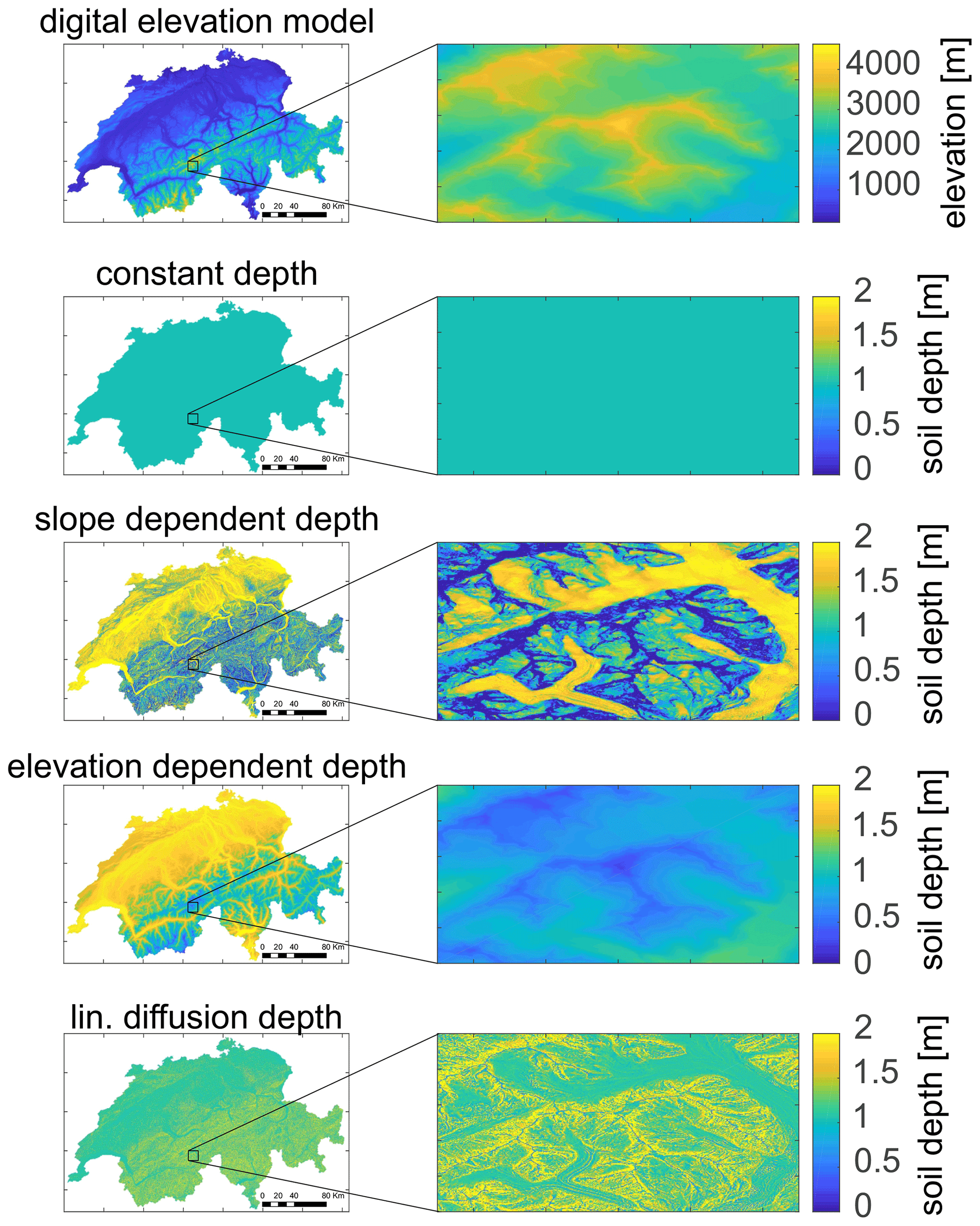
Figure 2From top to bottom: digital elevation model (DEM, Swisstopo 25 m) and four soil depth distributions: constant (d=1 m), slope- and elevation-dependent, and d between 0 and 2 m assuming the linear diffusion model at steady state. The maps on the right show a zoom-in view to the same area to appreciate small-scale variability.
These result in quite different spatial soil depth distributions, with the elevation-dependent soil depth mirroring the DEM, the slope-dependent soil depth showing low variability in depth in valleys and lowlands where slope is constant, and the linear diffusion model soil depth showing the highest spatial heterogeneity, with large differences in soil depth over short distances. This is due to the dependence on the second derivative of elevation (curvature) and results in low soil depth on mountain ridges but sometimes larger values in convergent topography right next to them.
We then compute the minimum (assuming soil completely wet, h=d in Eq. 1) and maximum (assuming soil completely dry, h=0 in Eq. 1) FoS for every 25 m × 25 m cell in Switzerland considering all four soil depth maps. We group the cells as unconditionally stable (when FoSmin>1), unconditionally unstable (when FoSmax<1), and conditionally (un)stable (all remaining cells) (Fig. 3). The resulting limits of the FoS over the country seem not to be affected strongly by the soil depth model chosen. This is confirmed also when looking at the fraction of cells with observed landslides in each condition (Table 1). Nevertheless this is not to say that soil depth is not an important parameter for the initiation of landslides, as in Fig. 3 and Table 1 we are not considering the interplay of soil depth and hydrology. Considering the two extreme scenarios (soil completely wet or completely dry), we are ignoring how likely these conditions are to occur and the fact that a thicker soil will likely be more difficult to saturate. Therefore, while soil depth does not seem to impact the areas with limiting conditions for completely wet and dry soil, it will very likely impact the landslide volume and the actual hydrological state and therefore FoS value.
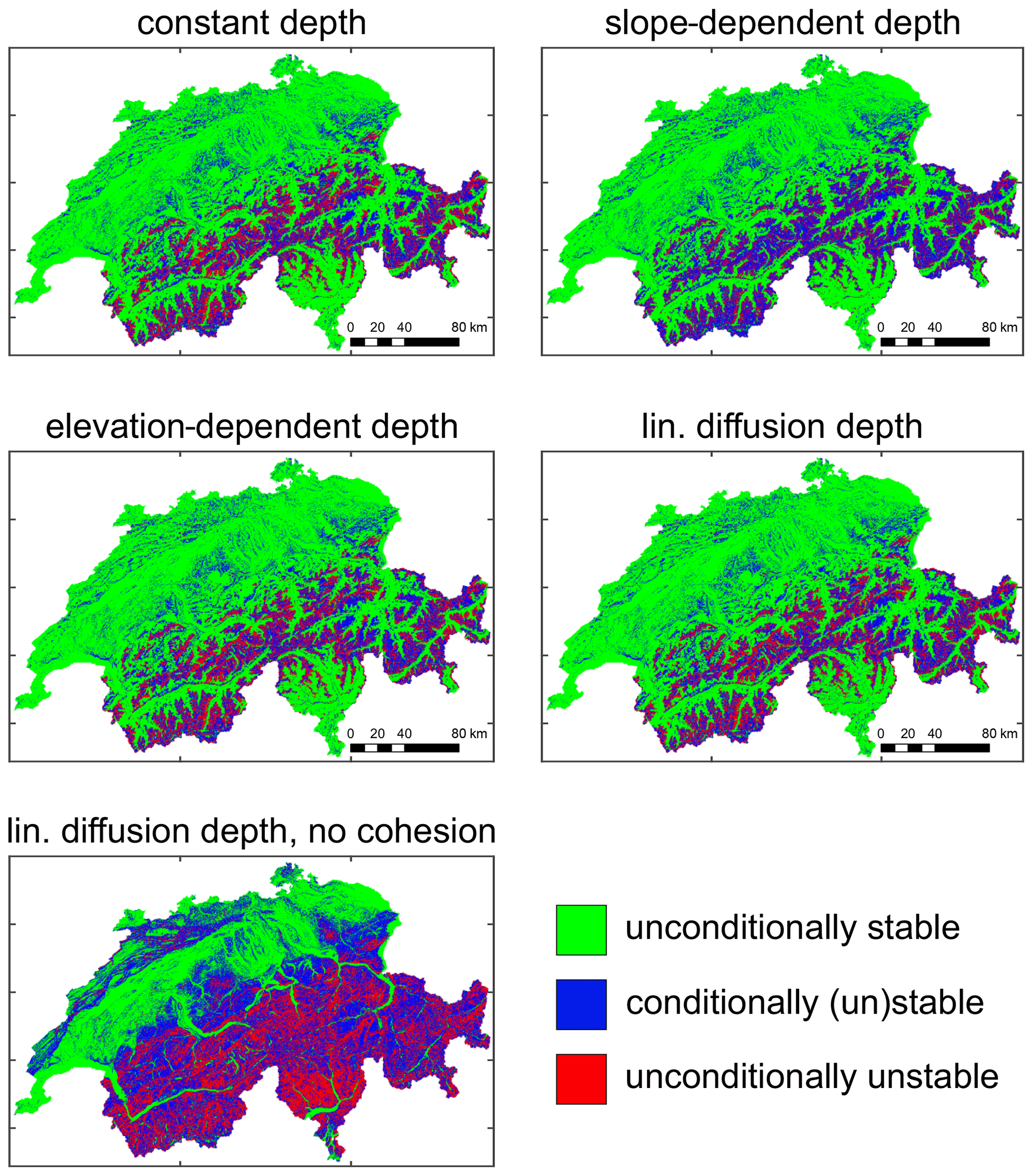
Figure 3Maps of (un)conditionally (un)stable regions of Switzerland obtained from the two factor of safety limiting cases (soil completely wet or dry) and the different soil depth models. Panel in the bottom row is the reference case obtained with the linear diffusion model neglecting cohesion (c=0).
Table 1Percentage of unconditionally stable (US), conditionally (un)stable (CUS), and unconditionally unstable (UU) cells in Switzerland according to the FoS calculations for each soil depth model and percentage of landslides in each condition from the landslide inventory. For the linear diffusion model, the results are also shown when cohesion is neglected (c=0).
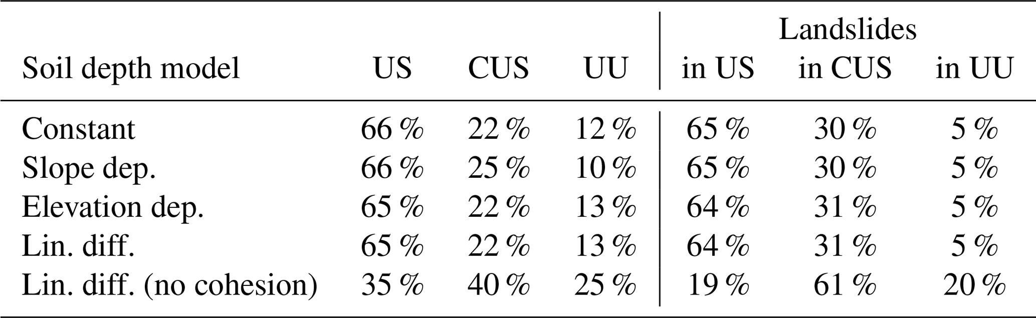
Under the conditions studied here, only 22 %–25 % of the area of Switzerland is conditionally unstable, i.e. area where hydrology matters for landslide occurrence according to the infinite slope model. The presence of so many landslides in unconditionally stable areas (65 %–66 % of the total number of landslides) and the existence of some unconditionally unstable cells (10 %–13 % of the country) are undesirable outcomes. While some inaccuracy in the location of the landslides (which might not refer to the detachment zone) could play a role, these results also suggest that either the infinite slope model is inadequate or that the input parameters are inaccurate. In fact, the sensitivity of the FoS to cohesion makes the point (Fig. 3 and Table 1) regarding parameter uncertainty. If we remove cohesion (c=0), a much larger portion of the country is susceptible to landslides (unstable or potentially unstable), and the hydrologically active portion, conditionally (un)stable, is now 40 % of the country, with more than 60 % of the total landslides recorded in this area, and only 19 % of the landslides remain in unconditionally unstable areas (Fig. 3 and Table 1). This is a strong indication that the infinite slope model predictions are highly sensitive to input parameters. These aspects and potential limitations of the FoS will be further discussed in Sect. 4.
3.1.2 The effect of dynamic hydrology
To address the temporal dynamics of FoS in the susceptible areas (25 m × 25 m cells where at least one landslide was recorded) and their connection to observed landslides, we extract the daily time series of simulated TerrSysMP soil water pressure for all TerrSysMP cells within Switzerland for the period 1989–2018, and we then compute the FoS in time for all 25 m × 25 m cells in which at least one landslide was recorded at the local depth estimated by the linear diffusion soil depth model.
The expectation is that landslides should occur when and where FoS < 1. While the value of 1 is often chosen as a theoretical threshold based on the balance of forces in a soil, several studies actually calibrate either the threshold FoS value or the critical area over which FoS < 1 in a region (e.g. Casadei et al., 2003). In this work we accept that the critical value of FoS can vary spatially depending on the soil parameters and the performance of the hydrological model. To this end, we focus on the departure of the FoS from the long-term temporal average of each cell. This allows us to focus only on the temporal dimension and observe whether the FoS is lower during triggering rainfall events (i.e. prior to landsliding). We compare the histograms of the departures in FoS from the local temporal mean of the triggering and non-triggering events (Fig. 4). While there is a clear trend of FoS being smaller than the mean (i.e. negative values) during triggering events more than non-triggering events, the separation is not sufficient to establish a warning system based on a threshold of FoS.
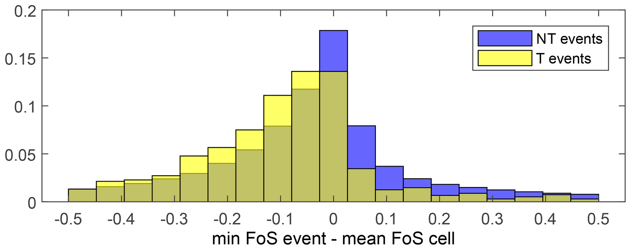
Figure 4Histograms of the departures of the minimum factor of safety from its grid-based long-term mean during landslide triggering (T) and non-triggering (NT) rainfall events, combining spatial (i.e. differences between landslide locations) and temporal (i.e. differences between events in the cells) variability.
In addition to soil pore water pressure and the FoS, we also consider the mean saturation over the top two model layers estimated by TerrSysMP and compare the departure of it from its long-term local temporal mean (Fig. 5a). This not only allows us to directly compare the estimates of the two modelling frameworks (PREVAH and TerrSysMP) but also to further assess the usefulness and validity of the infinite slope approach. For TerrSysMP, the difference between the departure from the mean during triggering and non-triggering events is barely noticeable for saturation. This suggests that although modelled TerrSysMP soil saturation by itself is not a good metric for a landslide warning system, its inclusion into a FoS with additional local soil and topography characteristics has some merit. Proof of this is the clearer separation between the distribution of values of triggering and non-triggering events for FoS departures from the mean (Fig. 4).
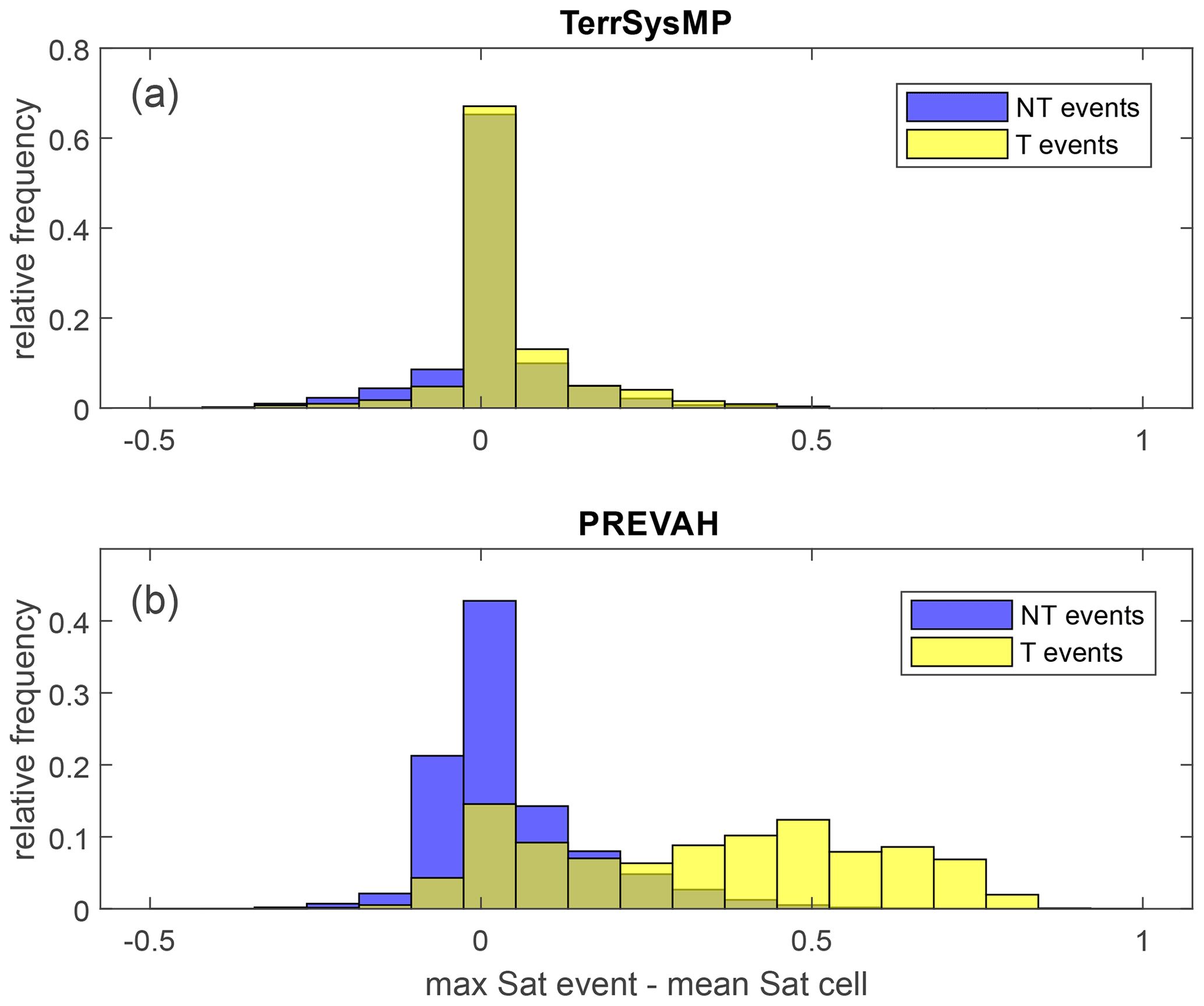
Figure 5Histograms of the departure of the maximum event saturation from its long-term local temporal mean for landslide triggering and non-triggering events, considering (a) saturation estimates from TerrSysMP and (b) from PREVAH.
3.2 Probabilistic approach
The role of antecedent wetness and the information content of the saturation estimates provided by the hydrological model PREVAH (Viviroli et al., 2009) for landslide prediction is explored in a similar way to the physically based approach, but because we do not have an estimate of soil pore water pressure in PREVAH, we use only soil saturation. We expect patterns opposite to that of the FoS: the saturation to be exceptionally large on landslide days and generally larger during triggering than non-triggering events. The separation of the distribution of the departure of saturation during triggering and non-triggering events from the local mean saturation (Fig. 5b) is evident and much clearer than for TerrSysMP. This suggests that the saturation estimate provided by PREVAH might contain information useful for the prediction of landslides. We explore this further by focusing on the misclassification associated with a rainfall threshold (i.e. false positives and false negatives). We first define the optimum ED threshold for landsliding by maximising the TSS (E=20.1D0.74, TSS = 0.68), and we then compute the average antecedent saturation for each duration and class of events: false positives, false negatives, true positives, and true negatives. Regardless of the number of days prior to the beginning of the rainfall event over which the mean saturation is computed, the false negatives (FNs, in Fig. 6) are always associated with the highest antecedent saturation, and the false positives (non-triggering events above the threshold, FPs in Fig. 6) with the lowest saturation. This confirms that at least some of the false negatives were triggered by a smaller rainfall amount than expected due to exceptionally high antecedent soil wetness, whereas sometimes, although the ED threshold was exceeded, no landslide event was observed due to exceptionally low saturation prior to the rainfall event. The only point for which the antecedent saturation prior to false negatives is not the highest is for duration of 6 d. However, this is due to the insufficient number of true negatives of such duration that are available (see dashed red line in the bottom right panel in Fig. 6).
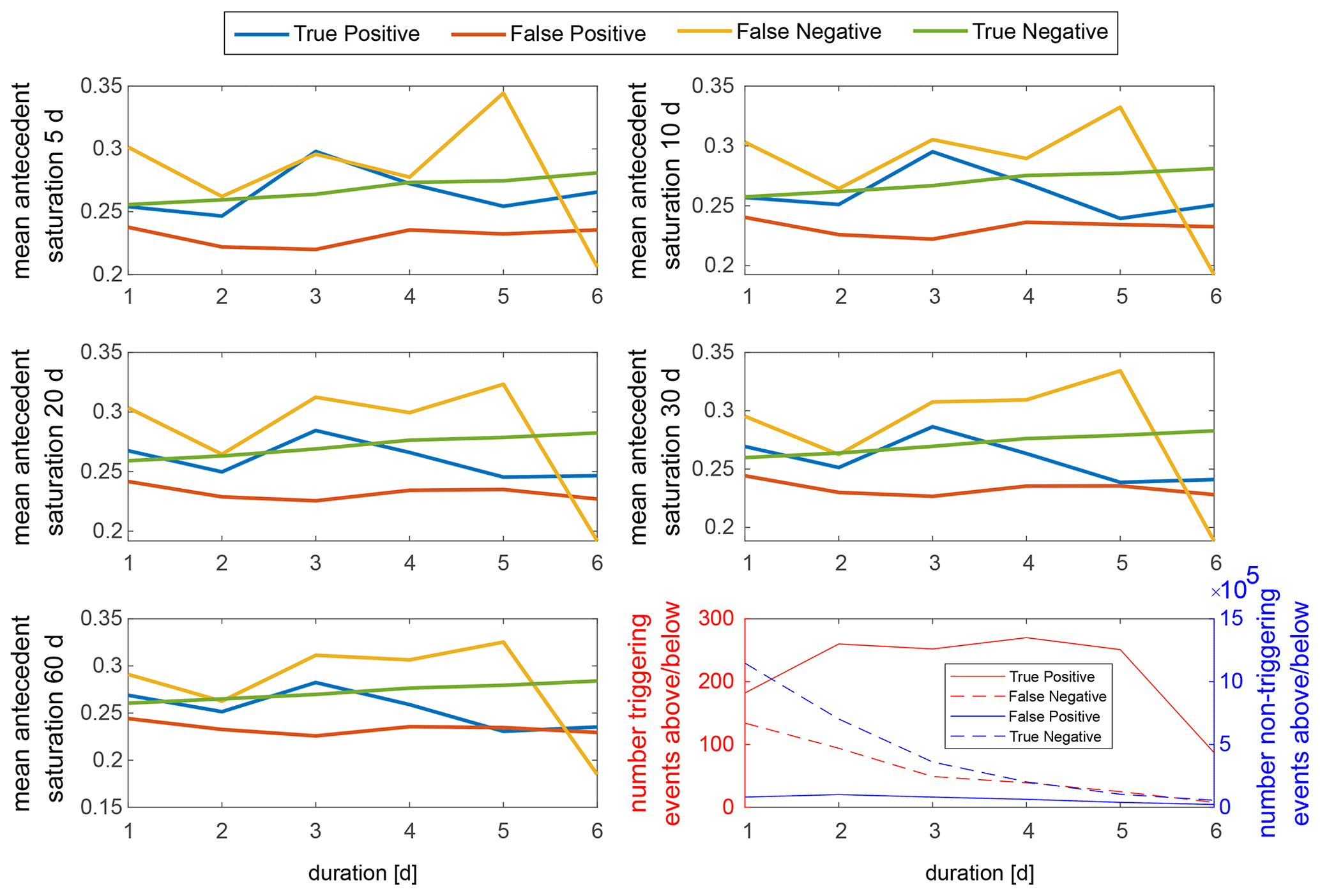
Figure 6Plots of mean antecedent soil saturation averaged over 5, 10, 20, 30, and 60 d prior to the beginning of the corresponding rainfall event for durations of 1–6 d. Events are divided into four groups: true positive (TP, triggering events above the threshold), false positive (FP, non-triggering events above the threshold, also called false alarms), false negative (FN, triggering events below the threshold, also called misses), and true negative (TN, non-triggering events below the threshold). The plot in the lower right shows the number of events in each group of events for each duration, to check the robustness of the mean estimates.
Based on these results, we consider two alternative approaches to combine antecedent saturation and rainfall characteristics for a landslide warning system. First we optimised thresholds by combining N d (N=1, 5, 10, 20, 30, 60 d) antecedent saturation with the logarithm of maximum daily rainfall, total rainfall, or mean daily intensity, in the shape of , where R is the rainfall characteristic, S the N d mean antecedent saturation, and a and b the parameters optimised by maximising TSS. The best performances are obtained with maximum daily rainfall intensity and 5 d antecedent saturation (Fig. 7), with a TSS of 0.67.
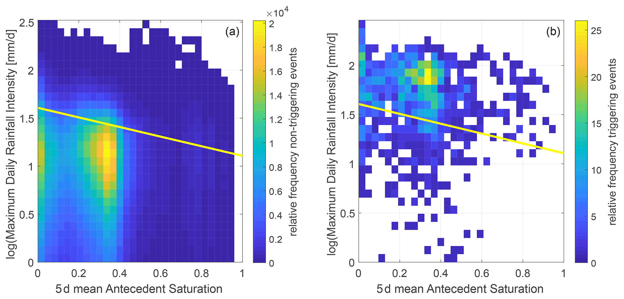
Figure 7Relative frequency plot of triggering (b) and non-triggering (a) events for the hydrometeorological threshold combining 5 d mean antecedent saturation and the logarithm of maximum daily intensity. The threshold leading to the highest TSS is indicated with a yellow line.
While these results show clearly the usefulness of antecedent soil saturation (i.e. smaller amounts of rainfall being necessary to trigger a landslide in wetter conditions), the performances are not superior to that of a standard rainfall threshold, which does not account for saturation. In fact, the total rainfall–duration (ED) threshold obtained, considering the same rainfall events, results in a maximum TSS of 0.68.
We therefore explored an alternative approach, where pure rainfall thresholds are defined but for different levels of antecedent soil saturation conditions, similarly to what Sidle and Ochiai (2006) did by splitting events according to antecedent rainfall. For this sequential thresholds approach, we first split the events according to the N d mean antecedent saturation and then utilised two different ED thresholds for wet (exceeding the saturation threshold) and dry (not exceeding it) conditions. Of the different antecedent periods and saturation thresholds considered, we find 10 d antecedent saturation with a 0.45 saturation threshold to lead to the best performances (Fig. 8 and to the ED thresholds shown in Fig. 9). It is interesting to notice that the parameters of the best thresholds for the wet () and dry () antecedent conditions suggest yet again that, at least for shorter duration events for which antecedent conditions are expected to be relevant, more rainfall is required to generate a landslide in dry conditions. The overall TSS value is 0.69, improving slightly upon the performances of pure rainfall thresholds. We propose this sequential threshold system as a candidate for the design of a regional warning system.
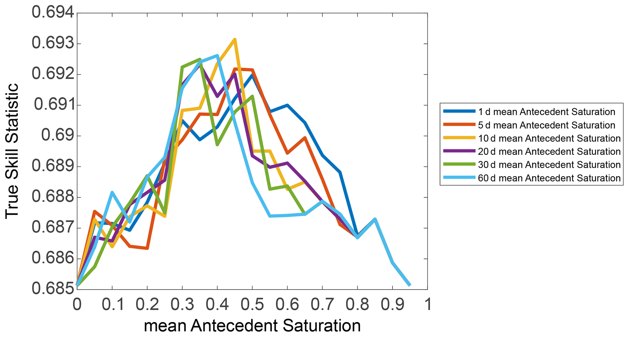
Figure 8True skill statistic values associated with the dual total rainfall–duration (ED) thresholds for high/low antecedent saturation conditions separated by thresholds of mean antecedent saturation (x axis). Colour lines represent different N d antecedent condition time frames.
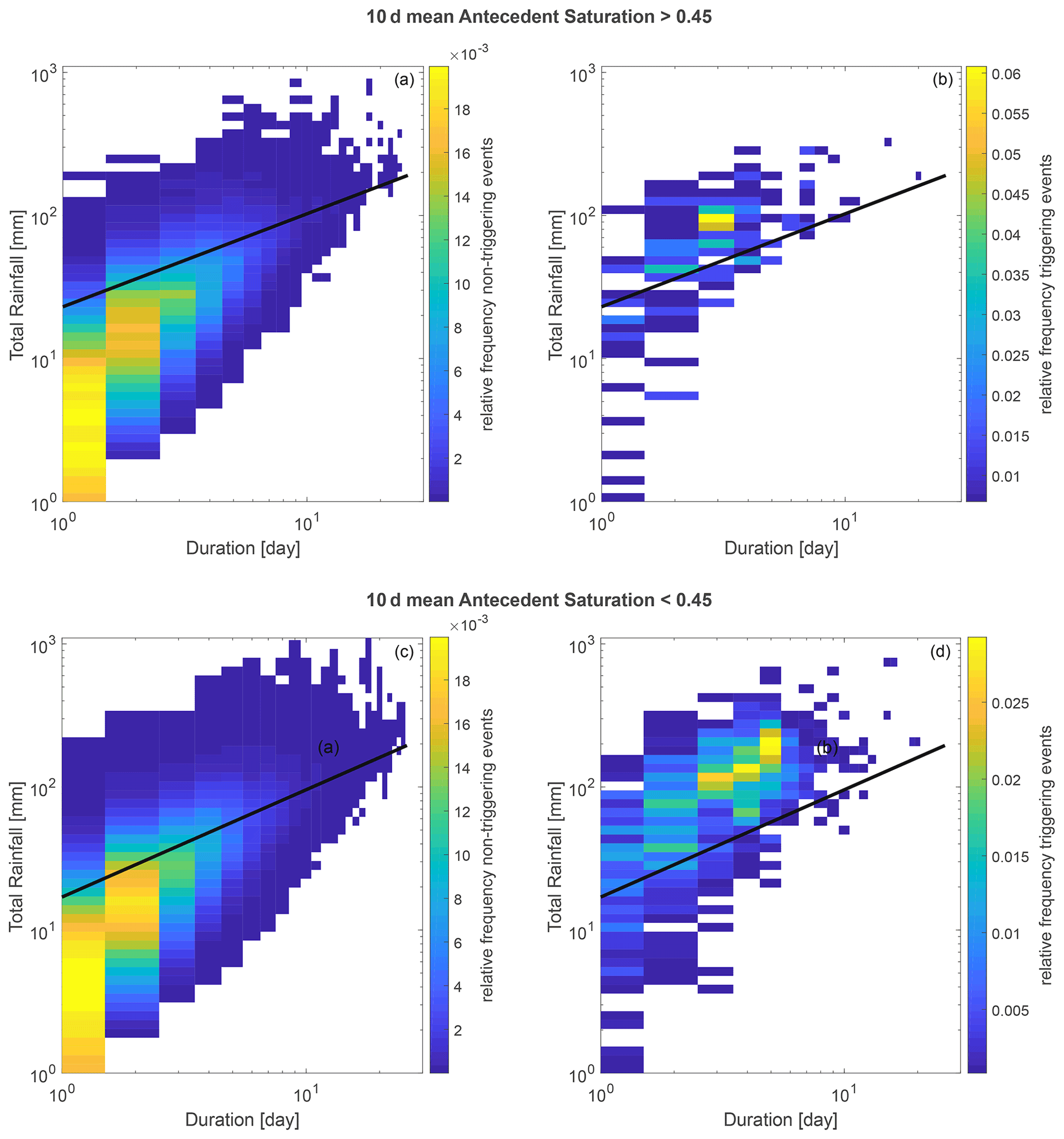
Figure 9Relative frequency plot of triggering (b, d) and non-triggering (a, c) events for the total rainfall–duration (ED) threshold above (a, b) and below (c, d) the soil saturation threshold of 0.45. The two ED thresholds curves are indicated as black lines in the upper panels, and their equations are in the text.
The results presented here suggest that the probabilistic approach with rainfall and soil saturation thresholds is superior to the physically based approach with the factor of safety calculation. It is important to stress that this is not a general statement but rather a conclusion drawn from the specific models and data which we compared. In fact, if a physically based approach would accurately capture the pore water pressure variations at the required high-resolution scales and therefore reproduce and predict slope failure with the FoS (or another geotechnical) model, we maintain that it would be superior to a probabilistic approach. It is therefore worthwhile to discuss the limitations of the tested physically based approach and the results obtained with regards to the geotechnical component (i.e. the infinite slope approach and FoS calculations) and those related to the hydrological component.
To consider the infinite slope approach independently from the hydrology, we can focus on the analysis of conditionally and unconditionally stable/unstable areas of Switzerland and their validation against the location of historical landslides. There are two concerning aspects in these results: the presence of many historical landslides (65 %–66 %) in unconditionally stable areas and the existence of unconditionally unstable areas. The uncertainty in the location of the landslides could explain some of the slope failures in unconditionally stable areas. Out of the 1354 landslides in unconditionally stable (US) areas, for 937 there are no US cells in the 24 neighbouring cells (area of 125 m × 125 m centred on the cell) and for 739 not even in the 80-cell neighbourhood (area of 275 m × 275 m centred on the cell). Furthermore, unconditionally unstable areas should theoretically not exist, because they should have failed already or have no soil. Nevertheless roughly 10 %–13 % of the country is classified as such. These two outcomes are therefore failures of the infinite slope approach and uncertainties in the soil parameters in the model. The FoS approach is based on strong simplifications and ignores potentially important processes such as suction in unsaturated soils, which temporarily increases stability. Nevertheless, we believe the uncertainties in the soil parameters have the strongest influence. Proof of this is the results obtained when neglecting apparent root cohesion (Fig. 3). The fact that the map of (un)conditional (in)stability changes considerably when removing cohesion shows the sensitivity of the FoS calculations to this parameter. Other input parameters may be similarly influential. For instance, the friction angle values obtained based on the soil texture map from OpenLandMap (Fig. 1b) are practically homogeneous over the country. We expect that friction angle is in reality much more heterogeneous and, together with cohesion, is affecting the unconditionally stable area. The sensitivity of the FoS estimates to the uncertain soil parameters can be examined theoretically or by Monte Carlo simulations, provided that parameter distributions are known (Hammond et al., 1992; Pack et al., 1998; Griffiths et al., 2011). Soil depth is also a very uncertain and influential parameter. The UU areas in the alpine region are very likely steep locations were the soil is absent (exposed bedrock). This aspect is missed by most soil datasets as well as soil depth models.
Another important aspect to consider for the FoS calculation is the spatial resolution. Higher resolutions allow models to better capture the local heterogeneities (if data are available), most importantly the topography (i.e. slope). On the other hand, at high resolutions, the assumption of slope length much greater than soil depth becomes invalid, and if the cell size becomes much smaller than the typical detachment area of landslides, the interactions between neighbouring cells become even more critical. For this reason, geotechnical models have been developed that explicitly model progressive failure, lateral interactions, and stress redistribution (Cohen et al., 2009; von Ruette et al., 2013; Anagnostopoulos et al., 2015; Fan et al., 2015).
The limitations of the hydrological component in the coarse-resolution TerrSysMP model, regardless of the geotechnical model, are evident from the very weak separation between triggering and non-triggering events in the FoS but even more in the soil saturation values themselves. In our analysis we focused on the temporal variability (i.e. departure from the local mean, for triggering and non-triggering events), and the only variable in the FoS calculation which can vary in time is the soil pore water pressure. This means that the lack of temporal variability in the FoS is a direct consequence of the lack of temporal variability in the water pressure head. While combining the hydrological estimates with the infinite slope approach does improve the separation compared to using saturation only, it is still insufficient to establish a threshold. The separation is instead mush stronger when considering soil saturation obtained from PREVAH.
Theoretically, a physically based model like TerrSysMP should be better capable of simulating the movement of water in the soil and therefore predicting the saturation or pressure more accurately. The lack of temporal variability in soil water distribution in TerrSysMP is evident in the large number of both triggering and non-triggering events for which the departure of maximum event saturation from the local mean saturation is 0 (bars for x=0 in Fig. 5a), suggesting the saturation is constant in time for those cells. We believe these results are a direct consequence of the spatial resolution of the model. In fact, at such coarse resolution, the model does not capture local changes driven by higher-resolution topography, e.g. lateral subsurface flow. At this coarse resolution, vertical fluxes in the soil will dominate over lateral fluxes (e.g. Lu et al., 2011). Simple downscaling techniques which can be used to increase the spatial resolution of models have been explored (e.g. TWI; Beven, 1995; Schmidt et al., 2008; Wang et al., 2020; Leonarduzzi et al., 2021), but because they are static, they would not affect the results shown here and compensate for the lack of temporal dynamics. If the coarse hydrological variable does not include enough temporal variability, neither will the higher-resolution spatially downscaled estimate. Another possible reason for the lack of spatial soil moisture variability in simulations is that most models assume a homogeneous single or multilayer soil without accounting for variable percolation and preferential flow at the soil–bedrock interface. This could reduce soil moisture variability even without accounting for lateral flow effects.
For the specific cases presented here, having a higher spatial resolution (500 m × 500 m rather than 12.5 km × 12.5 km) in a conceptual hydrological model seems more beneficial than the gain in accurate physical representation of the soil flow processes. This stresses once more the importance of adequate spatial resolution of hydrological models, especially for the assessment of slope and soil-saturation-dependent natural hazards such as landslides.
We explore two approaches for the prediction of landslides and the value of soil wetness in these predictions applied to a regional-scale study in Switzerland. In the first approach we use the soil water pressure estimates from a coarse-resolution physically based model (TerrSysMP) and slope stability assessment using the infinite slope approach. In the second approach we use rainfall–duration threshold curves informed by soil saturation obtained by a high-resolution conceptual hydrological model (PREVAH).
Our main findings are the following:
-
The infinite slope approach for quantifying slope instability is largely affected by the accuracy of input soil parameters, in particular cohesion in our case (removing cohesion doubled the area where hydrology mattered in FoS prediction), but the FoS can discern landslide triggering events better than soil moisture only by accounting for local topography and stress/strength balance.
-
According to the infinite slope approach and without considering parameter uncertainty, hydrology can play a role in the initiation of landslides over only ca. 20 % of Switzerland (the conditionally (un)stable area, where about 30 % of all observed landslides have occurred). Soil depth does not seem to affect the estimate of (un)conditionally (un)stable areas, although it is an essential parameter for the estimate of local wetness and determines the landslide volume.
-
Soil saturation estimates from a high-resolution conceptual hydrological model (PREVAH) are more useful in improving landslide predictions than those from a coarse-resolution physically based modelling framework (TerrSysMP), mainly due to effects related to the coarse spatial resolution of the latter model.
-
We suggest the use of sequential rainfall ED thresholds that first consider antecedent soil saturation conditions (with a optimal threshold of 10 d mean antecedent saturation of 0.45) and then different rainfall ED curves for wet and dry conditions.
The friction angle data were obtained from Geotechdata.info (Angle of Friction, http://geotechdata.info/parameter/angle-of-friction.html, as of 14 December 2013, last access: 7 July 2020). All other soil maps were downloaded from the OpenLandMap website (http://www.openlandmap.org, last access: 30 April 2020). The 25 m digital elevation model was provided by swisstopo (https://shop.swisstopo.admin.ch/en/products/height_models/dhm25, last access: 30 April 2020). The rainfall products were provided by the Swiss Federal Office of Meteorology and Climatology MeteoSwiss (available for research purposes upon request). The Swiss Federal Research Institute WSL provided the landslide data (available for research purposes upon request) and the PREVAH simulation results. TerrSysMP hydrological simulation results were downloaded from https://datapub.fz-juelich.de/slts/cordex/index.html (last access: 16 June 2020, https://doi.org/10.17616/R31NJMGR, re3data.org, 2021).
EL conducted the analysis. EL and PM conceived the research. All authors contributed to writing the paper.
The authors declare that they have no conflict of interest.
Publisher's note: Copernicus Publications remains neutral with regard to jurisdictional claims in published maps and institutional affiliations.
The authors thank Adrin Tohari and two anonymous referees, whose comments and suggestions in the revision helped improve and clarify this paper.
This research has been supported by the Swiss National Science Foundation (grant no. 165979).
This paper was edited by Carlo De Michele and reviewed by Adrin Tohari and two anonymous referees.
Aleotti, P. and Chowdhury, R.: Landslide hazard assessment: summary review and new perspectives, B. Eng. Geol. Environ., 58, 21–44, 1999. a
Anagnostopoulos, G. G., Fatichi, S., and Burlando, P.: An advanced process-based distributed model for the investigation of rainfall-induced landslides: The effect of process representation and boundary conditions, Water Resour. Research, 51, 7501–7523, https://doi.org/10.1002/2015WR016909, 2015. a, b
Anderson, S. A. and Sitar, N.: Analysis of rainfall-induced debris flows, J. Geotechn. Eng., 121, 544–552, 1995. a
Ayalew, L. and Yamagishi, H.: The application of GIS-based logistic regression for landslide susceptibility mapping in the Kakuda-Yahiko Mountains, Central Japan, Geomorphology, 65, 15–31, 2005. a
Baum, R. L., Savage, W. Z., and Godt, J. W.: TRIGRS – a Fortran program for transient rainfall infiltration and grid-based regional slope-stability analysis, US geological survey open-file report, 424, 38, https://doi.org/10.3133/ofr02424, 2002. a
Baum, R. L., Savage, W. Z., and Godt, J. W.: TRIGRS-A Fortran program for transient rainfall infiltration and grid-based regional slope-stability analysis, version 2.0, Tech. rep., US Geological Survey, https://doi.org/10.3133/ofr20081159, 2008. a, b
Beven, K.: Topmodel, in: Computer Models of Watershed Hydrology, Water Resour. Pub., edited by : Singh, V. P., 627–668, ISBN 0-918334-91-8, 1995. a
Bodeneignungskarte der Schweiz, Geodaten, 13147140, available at: https://www.bfs.admin.ch/bfs/en/home/services/geostat/swiss-federal-statistics-geodata/land-use-cover-suitability/derivative-complementary-data/swiss-soil-suitability-map.assetdetail.13147140.html, last access: July 2020. a
Bogaard, T. and Greco, R.: Invited perspectives: Hydrological perspectives on precipitation intensity-duration thresholds for landslide initiation: proposing hydro-meteorological thresholds, Nat. Hazards Earth Syst. Sci., 18, 31–39, https://doi.org/10.5194/nhess-18-31-2018, 2018. a, b
Brocca, L., Ponziani, F., Moramarco, T., Melone, F., Berni, N., and Wagner, W.: Improving landslide forecasting using ASCAT-derived soil moisture data: A case study of the Torgiovannetto landslide in central Italy, Remote Sens., 4, 1232–1244, 2012. a
Casadei, M., Dietrich, W., and Miller, N.: Testing a model for predicting the timing and location of shallow landslide initiation in soil-mantled landscapes, Earth Surf. Proc. Landf., 28, 925–950, 2003. a
Chung, C.-J. F., Fabbri, A. G., and Van Westen, C. J.: Multivariate regression analysis for landslide hazard zonation, in: Geographical information systems in assessing natural hazards, Springer, Dordrecht, 5, 107–133, https://doi.org/10.1007/978-94-015-8404-3_7, 1995. a
Cohen, D., Lehmann, P., and Or, D.: Fiber bundle model for multiscale modeling of hydromechanical triggering of shallow landslides, Water Resour. Res., 45, 1–20, https://doi.org/10.1029/2009WR007889, 2009. a, b
Dietrich, W. E. and Montgomery, D. R.: SHALSTAB: a digital terrain model for mapping shallow landslide potential, University of California, available at: http://calm.geo.berkeley.edu/geomorph/shalstab/index.htm (last access: June 2020), 1998. a
Dietrich, W. E., Reiss, R., Hsu, M.-L., and Montgomery, D. R.: A process-based model for colluvial soil depth and shallow landsliding using digital elevation data, Hydrol. Process., 9, 383–400, 1995. a, b
Dorren, L. and Schwarz, M.: Quantifying the stabilizing effect of forests on shallow landslide-prone slopes, in: Ecosystem-Based Disaster Risk Reduction and Adaptation in Practice, edited by: Renaud, F., Sudmeier-Rieux, K., Estrella, M., and Nehren, U., Springer, Cham, 42, 255–270, https://doi.org/10.1007/978-3-319-43633-3_11, 2016. a
Ermini, L., Catani, F., and Casagli, N.: Artificial neural networks applied to landslide susceptibility assessment, Geomorphology, 66, 327–343, 2005. a
Fan, L., Lehmann, P., and Or, D.: Effects of hydromechanical loading history and antecedent soil mechanical damage on shallow landslide triggering, J. Geophys. Res.-Earth Surf., 120, 1990–2015, 2015. a, b
Fan, L., Lehmann, P., and Or, D.: Effects of soil spatial variability at the hillslope and catchment scales on characteristics of rainfall-induced landslides, Water Resour. Res., 52, 1781–1799, https://doi.org/10.1002/2015WR017758, 2016. a
Formetta, G., Capparelli, G., and Versace, P.: Evaluating performance of simplified physically based models for shallow landslide susceptibility, Hydrol. Earth Syst. Sci., 20, 4585–4603, https://doi.org/10.5194/hess-20-4585-2016, 2016. a
Frei, C. and Schär, C.: A precipitation climatology of the Alps from high-resolution rain-gauge observations, Int. J. Climatol., 18, 873–900, https://doi.org/10.1002/(SICI)1097-0088(19980630)18:8<873::AID-JOC255>3.0.CO;2-9, 1998. a
Frei, C., Schöll, R., Fukutome, S., Schmidli, J., and Vidale, P. L.: Future change of precipitation extremes in Europe: Intercomparison of scenarios from regional climate models, J. Geophys. Res.-Atmos., 111, D06105, https://doi.org/10.1029/2005JD005965, 2006. a
Furusho-Percot, C., Goergen, K., Hartick, C., Kulkarni, K., Keune, J., and Kollet, S.: Pan-European groundwater to atmosphere terrestrial systems climatology from a physically consistent simulation, Sci. Data, 6, 1–9, 2019. a
Geotechdata.info, Angle of Friction: http://geotechdata.info/parameter/angle-of-friction, last access: 14 December 2013. a
Glade, T., Crozier, M., and Smith, P.: Applying probability determination to refine landslide-triggering rainfall thresholds using an empirical “Antecedent Daily Rainfall Model”, Pure Appl. Geophys., 157, 1059–1079, 2000. a
Godt, J. W., Baum, R. L., and Chleborad, A. F.: Rainfall characteristics for shallow landsliding in Seattle, Washington, USA, Earth Surf. Proc. Landf., 31, 97–110, 2006. a
Griffiths, D., Huang, J., and Fenton, G. A.: Probabilistic infinite slope analysis, Comput. Geotech., 38, 577–584, 2011. a
Guzzetti, F., Peruccacci, S., Rossi, M., and Stark, C. P.: Rainfall thresholds for the initiation of landslides in central and southern Europe, Meteorol. Atmos. Phys., 98, 239–267, https://doi.org/10.1007/s00703-007-0262-7, 2007. a
Hammond, C. J., Prellwitz, R. W., and Miller, S. M.: Landslide hazard assessment using Monte Carlo simulation, in: Proceedings of 6th international symposium on landslides, Christchurch, New Zealand, Balkema, 2, 251–294, 1992. a
Heimsath, A. M., Dietrich, W. E., Nishiizumi, K., and Finkel, R. C.: Stochastic processes of soil production and transport: Erosion rates, topographic variation and cosmogenic nuclides in the Oregon Coast Range, Earth Surf. Proc. Landf., 26, 531–552, 2001. a
Hengl, T., Mendes de Jesus, J., Heuvelink, G. B. M., Ruiperez Gonzalez, M., Kilibarda, M., Blagotić, A., Shangguan, W., Wright, M. N., Geng, X., Bauer-Marschallinger, B., Antonio Guevara, M., Vargas, R., MacMillan, R. A., Batjes, N. H., Leenaars, J. G. B., Ribeiro, E., Wheeler, I., Mantel, S., Kempen, B.: SoilGrids250m: Global gridded soil information based on machine learning, PLoS one, 12, e0169748, https://doi.org/10.1371/journal.pone.0169748, 2017. a
Highland, L. and Bobrowsky, P. T.: The landslide handbook: a guide to understanding landslides, US Geological Survey, Reston, 2008. a, b
Hilker, N., Badoux, A., and Hegg, C.: The Swiss flood and landslide damage database 1972–2007, Nat. Hazards Earth Syst. Sci., 9, 913–925, https://doi.org/10.5194/nhess-9-913-2009, 2009. a
Iverson, R. M.: Landslide triggering by rain infiltration, Water Resour. Res., 36, 1897–1910, 2000. a, b
Kjekstad, O. and Highland, L.: Economic and Social Impacts of Landslides, in: Landslides – Disaster Risk Reduction, edited by: Sassa, K. and Canuti, P., Springer, Berlin, Heidelberg, https://doi.org/10.1007/978-3-540-69970-5_30, 2009. a
Kurtz, W., He, G., Kollet, S. J., Maxwell, R. M., Vereecken, H., and Hendricks Franssen, H.-J.: TerrSysMP–PDAF (version 1.0): a modular high-performance data assimilation framework for an integrated land surface–subsurface model, Geosci. Model Dev., 9, 1341–1360, https://doi.org/10.5194/gmd-9-1341-2016, 2016. a
Lee, S. and Pradhan, B.: Landslide hazard mapping at Selangor, Malaysia using frequency ratio and logistic regression models, Landslides, 4, 33–41, 2007. a
Leonarduzzi, E. and Molnar, P.: Deriving rainfall thresholds for landsliding at the regional scale: daily and hourly resolutions, normalisation, and antecedent rainfall, Nat. Hazards Earth Syst. Sci., 20, 2905–2919, https://doi.org/10.5194/nhess-20-2905-2020, 2020. a
Leonarduzzi, E., Molnar, P., and McArdell, B. W.: Predictive performance of rainfall thresholds for shallow landslides in Switzerland from gridded daily data, Water Resour. Res., 53, 6612–6625, 2017. a, b, c, d, e, f
Leonarduzzi, E., Maxwell, R. M., Mirus, B. B., and Molnar, P.: Numerical Analysis of the Effect of Subgrid Variability in a Physically Based Hydrological Model on Runoff, Soil Moisture, and Slope Stability, Water Resour. Res., 57, e2020WR027326, https://doi.org/10.1029/2020WR027326, 2021. a
Lu, N. and Godt, J.: Infinite slope stability under steady unsaturated seepage conditions, Water Resour. Res., 44, W11404, https://doi.org/10.1029/2008WR006976, 2008. a
Lu, N., Kaya, B. S., and Godt, J. W.: Direction of unsaturated flow in a homogeneous and isotropic hillslope, Water Resour. Res., 47, W02519, https://doi.org/10.1029/2010WR010003, 2011. a
Marc, O., Gosset, M., Saito, H., Uchida, T., and Malet, J.-P.: Spatial patterns of storm-induced landslides and their relation to rainfall anomaly maps, Geophys. Res. Lett., 46, 11167–11177, 2019. a
Marino, P., Peres, D. J., Cancelliere, A., Greco, R., and Bogaard, T. A.: Soil moisture information can improve shallow landslide forecasting using the hydrometeorological threshold approach, Landslides, 17, 2041–2054, 2020. a
Mathew, J., Babu, D. G., Kundu, S., Kumar, K. V., and Pant, C.: Integrating intensity–duration-based rainfall threshold and antecedent rainfall-based probability estimate towards generating early warning for rainfall-induced landslides in parts of the Garhwal Himalaya, India, Landslides, 11, 575–588, 2014. a
Mirus, B. B., Jones, E. S., Baum, R. L., Godt, J. W., Slaughter, S., Crawford, M. M., Lancaster, J., Stanley, T., Kirschbaum, D. B., Burns, W. J., Schmitt, R. G., Lindsey, K. O., and McCoy, K. M.: Landslides across the USA: occurrence, susceptibility, and data limitations, Landslides, 17, 2271–2285, https://doi.org/10.1007/s10346-020-01424-4, 2020. a
Ohlmacher, G. C. and Davis, J. C.: Using multiple logistic regression and GIS technology to predict landslide hazard in northeast Kansas, USA, Eng. Geol., 69, 331–343, 2003. a
OpenLandMap: OpenLandMap, available at: http://www.openlandmap.org, last access: 30 April 2020. a
Pack, R. T., Tarboton, D. G., and Goodwin, C. N.: The SINMAP approach to terrain stability mapping, in: 8th congress of the international association of engineering geology, Vancouver, British Columbia, Canada, 21, 25, 1998. a, b
Petley, D.: Global patterns of loss of life from landslides, Geology, 40, 927–930, 2012. a
Ponziani, F., Pandolfo, C., Stelluti, M., Berni, N., Brocca, L., and Moramarco, T.: Assessment of rainfall thresholds and soil moisture modeling for operational hydrogeological risk prevention in the Umbria region (central Italy), Landslides, 9, 229–237, https://doi.org/10.1007/s10346-011-0287-3, 2012. a
re3data.org: Data Publication Server Forschungszentrum Jülich, editing status 2020-09-02, re3data.org – Registry of Research Data Repositories [data set], https://doi.org/10.17616/R31NJMGR, 2021. a
Reichenbach, P., Rossi, M., Malamud, B. D., Mihir, M., and Guzzetti, F.: A review of statistically-based landslide susceptibility models, Earth-Sci. Rev., 180, 60–91, 2018. a, b
Roering, J. J.: How well can hillslope evolution models “explain” topography? Simulating soil transport and production with high-resolution topographic data, Geol. Soc. Am. B., 120, 1248–1262, 2008. a, b
Saito, H., Nakayama, D., and Matsuyama, H.: Comparison of landslide susceptibility based on a decision-tree model and actual landslide occurrence: the Akaishi Mountains, Japan, Geomorphology, 109, 108–121, 2009. a
Salvati, P., Bianchi, C., Rossi, M., and Guzzetti, F.: Societal landslide and flood risk in Italy, Nat. Hazards Earth Syst. Sci., 10, 465–483, https://doi.org/10.5194/nhess-10-465-2010, 2010. a
Saulnier, G.-M., Beven, K., and Obled, C.: Including spatially variable effective soil depths in TOPMODEL, J. Hydrol., 202, 158–172, 1997. a, b
Schmidt, J., Turek, G., Clark, M. P., Uddstrom, M., and Dymond, J. R.: Probabilistic forecasting of shallow, rainfall-triggered landslides using real-time numerical weather predictions, Nat. Hazards Earth Syst. Sci., 8, 349–357, https://doi.org/10.5194/nhess-8-349-2008, 2008. a, b
Schwarz, M., Cohen, D., and Or, D.: Spatial characterization of root reinforcement at stand scale: theory and case study, Geomorphology, 171, 190–200, 2012. a
Segoni, S., Piciullo, L., and Gariano, S. L.: A review of the recent literature on rainfall thresholds for landslide occurrence, Landslides, 15, 1483–1501, 2018. a
Shepard, D. S.: Computer Mapping: The SYMAP Interpolation Algorithm, in: Spatial Statistics and Models. Theory and Decision Library (An International Series in the Philosophy and Methodology of the Social and Behavioral Sciences), edited by: Gaile, G. L. and Willmott, C. J., Springer, Dordrecht, 40, https://doi.org/10.1007/978-94-017-3048-8_7, 1984. a
Sidle, R. and Ochiai, H.: Processes, prediction, and land use, Water resources monograph. American Geophysical Union, Washington, 2006. a, b
Stähli, M., Sättele, M., Huggel, C., McArdell, B. W., Lehmann, P., Van Herwijnen, A., Berne, A., Schleiss, M., Ferrari, A., Kos, A., Or, D., and Springman, S. M.: Monitoring and prediction in early warning systems for rapid mass movements, Nat. Hazards Earth Syst. Sci., 15, 905–917, https://doi.org/10.5194/nhess-15-905-2015, 2015. a
Thomas, M. A., Mirus, B. B., and Collins, B. D.: Identifying physics-based thresholds for rainfall-induced landsliding, Geophys. Res. Lett., 45, 9651–9661, 2018. a
Thomas, M. A., Collins, B. D., and Mirus, B. B.: Assessing the feasibility of satellite-based thresholds for hydrologically driven landsliding, Water Resources Research, 55, 9006–9023, 2019. a
Trezzini, F., Giannella, G., and Guida, T.: Landslide and Flood: Economic and Social Impacts in Italy, Springer, 2, 171–176, https://doi.org/10.1007/978-3-642-31313-4_22, 2013. a
Viviroli, D., Zappa, M., Gurtz, J., and Weingartner, R.: An introduction to the hydrological modelling system PREVAH and its pre-and post-processing-tools, Environ. Model. Softw., 24, 1209–1222, 2009. a, b, c
von Ruette, J., Papritz, A., Lehmann, P., Rickli, C., and Or, D.: Spatial statistical modeling of shallow landslides–validating predictions for different landslide inventories and rainfall events, Geomorphology, 133, 11–22, 2011. a
von Ruette, J., Lehmann, P., and Or, D.: Rainfall-triggered shallow landslides at catchment scale: Threshold mechanics-based modeling for abruptness and localization, Water Resour. Res., 49, 6266–6285, 2013. a, b
Wang, S., Zhang, K., van Beek, L. P., Tian, X., and Bogaard, T. A.: Physically-based landslide prediction over a large region: Scaling low-resolution hydrological model results for high-resolution slope stability assessment, Environ. Model. Softw., 124, 104607, https://doi.org/10.1016/j.envsoft.2019.104607, 2020. a, b
Wicki, A., Lehmann, P., Hauck, C., Seneviratne, S. I., Waldner, P., and Stähli, M.: Assessing the potential of soil moisture measurements for regional landslide early warning, Landslides, 17, 1881–1896, 2020. a
Yilmaz, I.: Landslide susceptibility mapping using frequency ratio, logistic regression, artificial neural networks and their comparison: a case study from Kat landslides (Tokat–Turkey), Comput. Geosci., 35, 1125–1138, 2009. a, b