Evaluating different machine learning methods to simulate runoff from extensive green roofs

Green roofs are increasingly popular measures to permanently reduce or delay storm-water runoff. The main objective of the study was to examine the potential of using machine learning (ML) to simulate runoff from green roofs to estimate their hydrological performance. Four machine learning methods, artificial neural network (ANN), M5 model tree, long short-term memory (LSTM) and k nearest neighbour (kNN), were applied to simulate storm-water runoff from 16 extensive green roofs located in four Norwegian cities across different climatic zones. The potential of these ML methods for estimating green roof retention was assessed by comparing their simulations with a proven conceptual retention model. Furthermore, the transferability of ML models between the different green roofs in the study was tested to investigate the potential of using ML models as a tool for planning and design purposes. The ML models yielded low volumetric errors that were comparable with the conceptual retention models, which indicates good performance in estimating annual retention. The ML models yielded satisfactory modelling results (NSE >0.5) in most of the roofs, which indicates an ability to estimate green roof detention. The variations in ML models' performance between the cities was larger than between the different configurations, which was attributed to the different climatic characteristics between the four cities. Transferred ML models between cities with similar rainfall events characteristics (Bergen–Sandnes, Trondheim–Oslo) could yield satisfactory modelling performance (Nash–Sutcliffe efficiency NSE >0.5 and percentage bias |PBIAS| <25 %) in most cases. However, we recommend the use of the conceptual retention model over the transferred ML models, to estimate the retention of new green roofs, as it gives more accurate volume estimates. Follow-up studies are needed to explore the potential of ML models in estimating detention from higher temporal resolution datasets.

1 Introduction

Green roofs are a type of green infrastructure (GI) that have received significant attention in recent years. In contrast to conventional storm-water infrastructure, green roofs attempt to decrease storm-water outflows while providing other services, such as reducing urban heat island effect, preserving the cities ecosystems and improving the urban visual amenity among other benefits (Berndtsson, 2010). Roof areas represent around 40 %–50 % of impermeable areas in dense urban catchments (Dunnett and Kingsbury, 2004); therefore, retrofitting current roofs with substrate/growing media and vegetation offers an efficient and area-free GI option. Many studies have confirmed the potential of green roofs to mitigate rainfall events from field measurements (Fassman-Beck et al., 2013; Johannessen et al., 2018; Liu and Chui, 2019; Stovin, 2010).

Quantifying the hydrological performance of a green roof is usually done by estimating “retention”, a permanent reduction of storm water by evapotranspiration, and “detention”, flow peak reduction and delay. Both retention and detention metrics are needed to justify the widespread implementation of green roofs by the storm-water community and for planning and design by practicing engineers. Hence, numerous studies have investigated different approaches and tools to simulate outflows from green roofs to estimate retention and detention metrics.

For estimating green roof detention, models that simulate rainfall–runoff events in short time steps (sub-hourly) are required. Several models have been tested successfully in the literature, which can be categorized into physically based and conceptual models. Physically based models simulate the water flow in porous media by solving physical equations numerically, such as the Richards equations, either in 1D (Bouzouidja et al., 2018; Liu and Fassman-Beck, 2017; Peng et al., 2019), 2D (Li and Babcock, 2015; Palla et al., 2009) or 3D (Brunetti et al., 2016). Several tools exist that can be used to implement this type of model, such as HYDRUS (Simunek et al., 2005), SWMS-2D (Simunek et al., 1994) and COMSOL Multiphysics (Multiphysics, 2013; Sims et al., 2019). These models have proven to be accurate and to rely only on measurable parameters (Sims et al., 2019) and can be powerful tools for studies that aim at in-depth understanding of the hydraulic behaviours of the different green roof layers (Brunetti et al., 2016).

Another category of physically based models apply simplified and analytical forms of physical equations, such as the Green–Ampt equation for infiltration and the Darcy law for saturated water flow (Krebs et al., 2016; She and Pang, 2010; Hernes et al., 2020). Popular modelling tools that implement these models include the EPA-SWMM (Rossman et al., 2010) and MIKE URBAN (DHI, 2017). This category of models is perhaps the most commonly applied in the literature of green roof modelling, and it has been acknowledged by many studies to be a suitable tool for analysing the hydrological performance of green roofs (Cipolla et al., 2016). However, due to the simplicity of these models, they often rely on calibrated rather than measured parameters. Peng and Stovin (2017) found the simulated hydrographs of uncalibrated SWMM models to deviate significantly form the observed ones. Johannessen et al. (2019) attempted to transfer calibrated SWMM model parameters between similar green roofs located in different locations. However, only parameter sets from wet locations yielded good results in drier locations but not vice versa

Conceptual models simplify the physical processes using linear or nonlinear equations to simulate green roof runoff. One common type of these models is the reservoir routing model which was applied to estimate runoff detention from event-based simulations in previous literature (Palla et al., 2012; Soulis et al., 2017; Vesuviano et al., 2014). These models were found to produce results that are comparable to physically based models with lower level of complexity (i.e. reduced number of model parameters) (Peng et al., 2019). Palla et al. (2012) recommended the use of a reservoir routing model instead of physically based models for design purposes when little information is available about the green roof properties. However, the parameters of conceptual models are not measurable. Hence, calibration is needed to find their optimal values, unlike physically based models (Peng et al., 2019). A few studies have identified relations between the flow parameters of reservoir models and some physical properties of green roofs, such as slope and substrate depth (Vesuviano and Stovin, 2013; Yio et al., 2013). However, these studies focused on lab-scale green roofs in which detention due to the horizontal flow is not significant (Sims et al., 2019).

For estimating green roof retention, models with water balance equations (in hourly or daily time step) and suitable representation of the actual evapotranspiration process (AET) were found by many studies to be sufficient (Bengtsson et al., 2005; Jahanfar et al., 2018; Johannessen et al., 2017; Stovin et al., 2013). The most common way to model AET is by multiplying the potential evapotranspiration (PET), the maximum evaporation rate assuming unlimited water supply, with reduction functions that account for soil moisture deficit and crop type. The reduction functions require careful parameterization of the maximum storage of the roof and crop factors. The maximum storage of the roof was found by many studies to be related to the measurable field capacity of the substrate (Liu and Fassman-Beck, 2017; Stovin et al., 2013). Crop factors for agricultural crops are well documented and studied (Allen et al., 1998). However, crop factor values for Sedum plants, commonly applied for green roofs, are less known. Previous studies reported different crop factor values for Sedum plants (Berretta et al., 2014; Rezaei et al., 2005; Sherrard and Jacobs, 2012).

Data-driven models, which are derived entirely from observed data, may offer alternative modelling tools that can estimate both retention and detention of green roofs without explicitly accounting for complex hydrological processes. However, the use of data-driven models in green roof studies has been limited to simple regression models (Carson et al., 2013) which are site-specific and not transferable. More advanced data-driven methods, such as machine learning (ML), have been commonly applied in many hydrological modelling studies in the last few decades. However, only a few studies were found to apply ML models in green infrastructures (Tsang and Jim, 2016; Radfar and Rockaway, 2016; Li et al., 2019), and no study was found to apply ML models in estimating the hydrological performance of extensive green roofs.

Machine learning methods have been successfully applied in hydrological modelling in recent decades. Previous studies reported better performances of ML models compared to conventional hydrological models in runoff prediction (Solomatine and Dulal, 2003; Yilmaz and Muttil, 2014; Young et al., 2017), runoff simulation (Javan et al., 2015; Kratzert et al., 2018), and for building relationships between water level and discharge (Bhattacharya and Solomatine, 2005). Some of the popular machine learning methods applied in hydrology include artificial neural networks (ANNs), M5 model tree, long short-term memory (LSTM) and k nearest neighbour (kNN).

Artificial neural network is the most common and among the earliest ML used in hydrological modelling (Daniell, 1991). Early examples of research into ANN include the study conducted by Hsu et al. (1995), in which ANN outperformed the linear ARMAX and the conceptual Sacramento SAC-SMA model in simulating runoff from a medium-sized catchment. Likewise, Tokar and Johnson (1999) compared an ANN to a simple conceptual model and found the former to outperform the latter. M5 model tree has been applied in different studies. Solomatine and Dulal (2003) reported a satisfactory performance of both M5 model tree and ANN in runoff forecasting. They, however, emphasized the advantages of M5 model tree over ANN due to the better interpretation of M5 model outputs. Goyal et al. (2013b) applied the M5 model tree for flow forecasting in India, among other ML methods, and found it to perform satisfactorily. Away from flow simulation, Gharaei-Manesh et al. (2016) used M5 tree and other methods to simulate the spatial distribution of snow depths in Iran, while Goyal et al. (2013a) evaluated M5 model tree on formulating operation rules for a reservoir. Kisi (2016) used M5 model tree to model reference evapotranspiration.

LSTM has been applied in different scientific fields and could provide good results (Shen, 2018). Regarding runoff modelling, Kratzert et al. (2018) investigated the potential of LSTM to predict runoff from ungauged basins. They could achieve good prediction performance that was comparable to the well-known Sacramento model. Similarly, Ayzel (2019) obtained comparable results with LSTM to a conceptual model. Hu et al. (2018) compared between an ANN and an LSTM in runoff simulation and found the latter to outperform the former. Nevertheless, LSTM is computationally expensive, and the training process takes a long time (Ayzel, 2019). The k nearest neighbour method was applied first by Karlsson and Yakowitz (1987) in runoff forecasting in which it outperformed unit hydrograph forecasters. Modaresi et al. (2018) found the k nearest neighbour to be comparable with ANN in monthly runoff forecasting. Furthermore, Wu et al. (2009) applied the k nearest neighbour in predicting monthly runoff, and they discussed the effect of k value on the performance of kNN.

Few studies have modelled green infrastructure with ML techniques. For instance, Tsang and Jim (2016) applied a Fuzzy-neural network to optimize irrigation of a green roof by estimating soil moisture deficit. The neural network could reproduce the soil moisture well, which indicates the capability of ML models to simulate the nonlinear AET process. Li et al. (2019) developed an artificial neural network model to predict the flow reduction from a catchment with different GI structures. Similarly, Radfar and Rockaway (2016) applied a neural network model to predict flow reduction from a permeable pavement. The satisfactory performances of ML models in two studies demonstrate the potential of ML models in GI hydrological modelling.

This study examines the ability of four machine learning methods, M5 model tree, artificial neural networks (ANNs), long short-term memory (LSTM) and k nearest neighbour (kNN), to estimate green roof hydrological performance specifically by

1. evaluating the performance of ML models in simulating the temporal dynamics of green roof subsurface runoff and estimating the retention from long-term simulations across different climatic locations;

2. investigating the potential of using ML models as a useful tool for planning that predicts the performance of new green roofs when observations are not available.

2 Data

Sixteen extensive green roofs located in four Norwegian cities with different climates – Bergen (BERG), Sandnes (SAN), Oslo (OSL) and Trondheim (TRD) – were used in the study. Bergen city is located on the western coast of Norway. Bergen is the wettest city among the four with annual precipitation of 3110 mm followed by Sandnes city, which is located on the south-west coast, with annual precipitation of 1690 mm. Oslo is the driest city with only 970 mm of annual precipitation, while Trondheim is the northernmost city with annual precipitation of 1070 mm. According to the Köppen–Geiger climate classification (Kottek et al., 2006), both Bergen and Sandnes are classified as temperate oceanic climate (Cfb), while Oslo has the warm-summer humid continental climate (Dfb), and Trondheim has a subpolar oceanic climate (Dfc). The locations of the four cities are shown in Fig. 1.

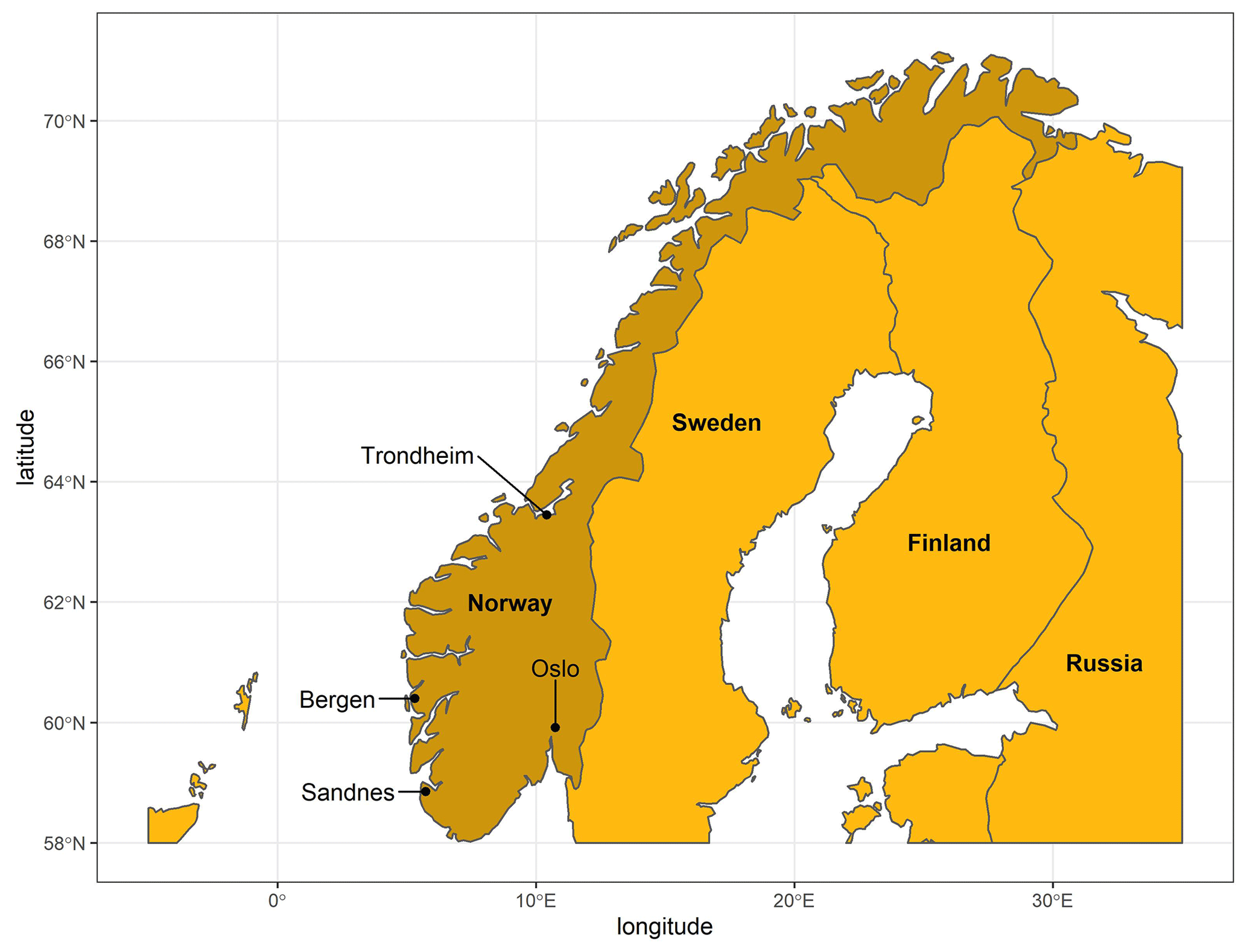
Figure 1 Locations of the four Norwegian cities with green roof field data.

Table 1 shows the geometries and configurations of roofs. Roof geometries (areas and slopes) vary between the cities, while the different configurations represent the variety of options in the Norwegian green roof market. Some green roofs in the study have the same configuration, for instance, BERG1, SAN1 OSL3 and TRD1. Continuous time series data were collected from TRD, BERG and SAN roofs between 2015 to 2017, while the green roofs at OSL have a 7-year record of data from 2011 to 2017. Data includes precipitation, runoff, relative humidity and wind speed at a 1 min resolution. In Oslo, the wind speed was not measured at the roofs but collected from a nearby station. For details about roof setup, data collection and processing, please refer to Johannessen et al. (2018).

Table 1 Roof Geometries and Configurations.

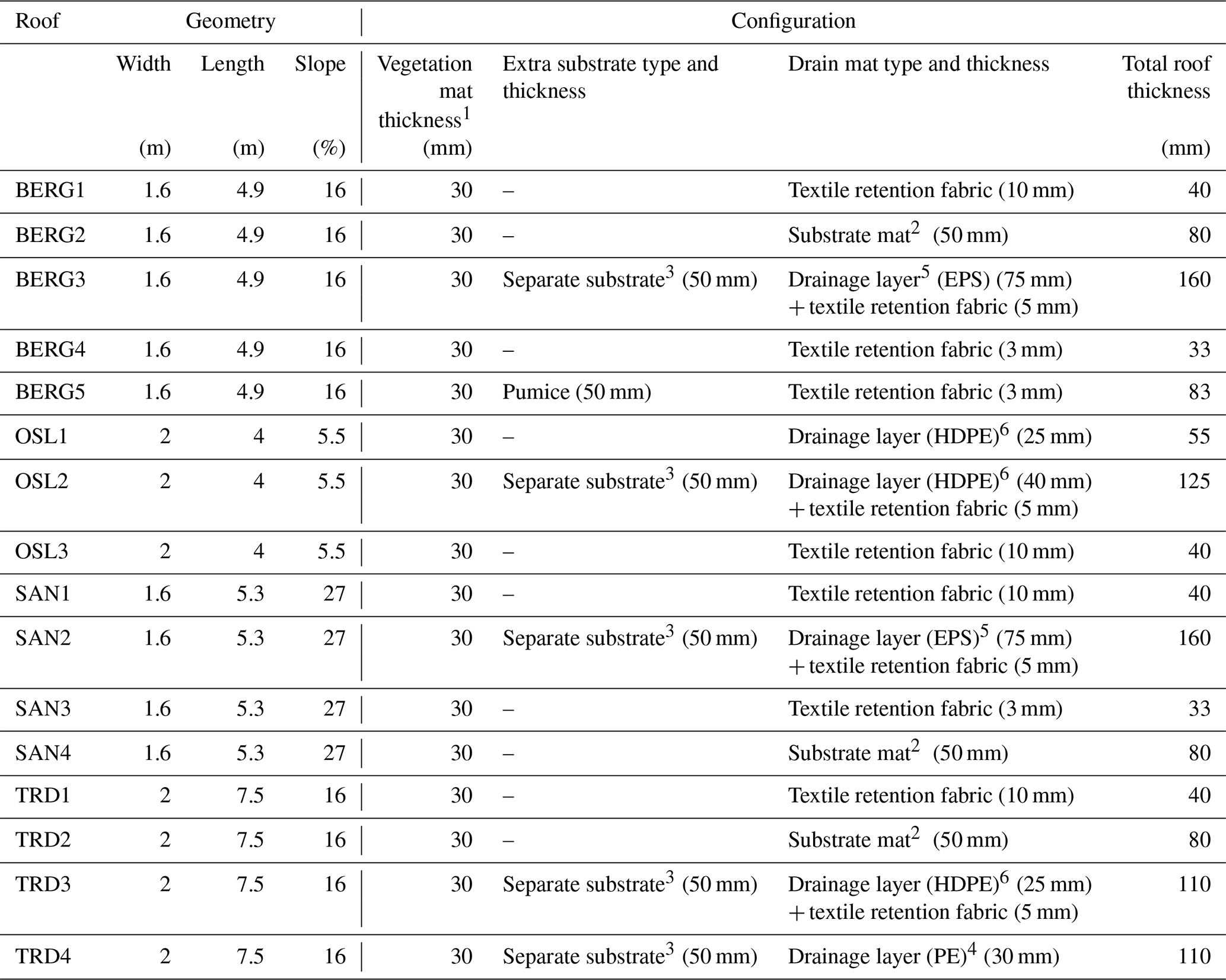
¹Pregrown reinforced vegetation mats (sedum).
²Substrate mat: a mineral wool plate.
³Separate substrate: a mixture of LECA and bricks.
⁴Drainage layer (PE): plastic drainage layers of polyethylene.
⁵Drainage layer (EPS): plastic drainage layers of expanded polystyrene.
⁶Drainage layer (HDPE): plastic drainage layers of high-density polyethylene.

3 Methods and tools

3.1 Machine learning models

3.1.1 M5 model tree

In this approach, the training data are divided into many subsets. For each subset, a piecewise linear regression equation is built between the output and the input variables (Solomatine and Dulal, 2003). The algorithm used by the model tree is called M5, which was developed in 1992 (Quinlan et al., 1992). It divides the data into subsets based on rules that reduce the intra-variation (variance) within each subset (variables within each subset are as similar as possible). The M5 model tree has an upside-down tree structure. Input variables enter the tree from the top (the tree root) to arrive at the models located at the tree leaves. For a detailed explanation of the M5 model tree, see Solomatine and Dulal (2003).

In this study, the Cubist library in R (Kuhn et al., 2012) was used to build M5 models. The performance of Cubist-M5 models can be improved by tuning two hyperparameters, namely committees and neighbours. The former is the number of trees in a boost-like ensemble scheme where iterative M5 model trees are built in sequence. The first M5 tree is built following the M5 algorithm, while the subsequent trees are created from the residuals of the single tree. The final model prediction is the average from all M5 trees in the ensemble. The final prediction of a single tree can be improved by a post-model nearest-neighbour adjustment (Quinlan, 1993). The predicted value of the tree is smoothed following a weighting schemes from several nodes within the single tree. The number of nodes used in the smoothing is called neighbours.

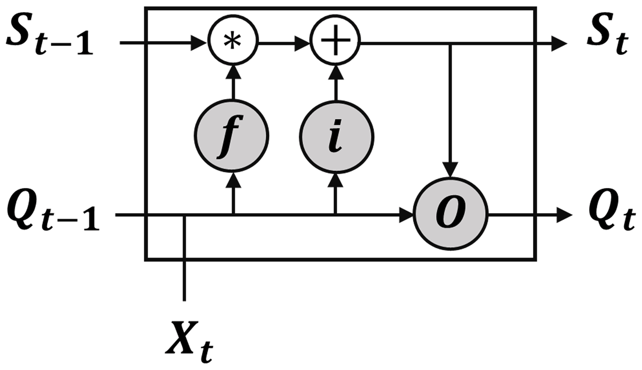
Figure 2 Structure of the long short-term memory (LSTM) cell, modified from (Kratzert et al., 2018).

3.1.2 Artificial neural network (ANN)

The ANN applied in this study is the standard feed-forward neural network. It comprises an input layer, a hidden layer(s) and an output layer. The building block of the network is called a neuron, and each neuron is fully connected with all other neurons in the backward and forward layers. Hidden layers are where relations between input variables are revealed. Each neuron in the ANN applies simple mathematical operations for the variable vectors, as represented in Eq. (1):

$$\begin{array}{}\text{(1)}& O=f(X\mathrm{1}\times W\mathrm{1}+X\mathrm{2}\times W\mathrm{2}+B)\end{array}$$

O is the output from a neuron; W1 and W2 are the weights of the variables X1 and X2, respectively; and B is the neuron's bias. f(.) is the neuron's activation function that adds nonlinearity to the neuron's output. During the training process, the weights and biases are updated for the whole network to obtain the best fit between simulated and observed outputs. A standard algorithm used for the training is backpropagation, which uses the approach of the steepest gradient descent (Rumelhart et al., 1986). Training of the neural network is done by dividing the training dataset into several batches. The weights and biases are updated for each batch until all training data have been visited, and then the same cycle is repeated. This cycle is called an epoch, and the learning performance improves with the increasing number of epochs. However, there is a risk of overfitting for models with high numbers of epochs. To avoid that, a separate dataset (validation dataset) is often used to optimize the number of epochs by determining the objective function for the validation data while training the model. Overfitting starts when the error increases in the validation dataset while decreasing in the training data.

3.1.3 Long short-term memory (LSTM)

In hydrology, sequential runoff data are often autocorrelated, especially data with a short time step. Autocorrelation is triggered by system memory in hydrology, usually due to the storage effects. A recurrent neural network (RNN) is a special type of neural networks that can tackle sequential data modelling because it includes output from the previous time step as input to the following time step. Nevertheless, it does not account for the long-term dependency in the system. Hochreiter and Schmidhuber (1997) discussed the issue of RNN with long-term dependency and proposed a unique RNN model called long short-term memory (LSTM). In this model, a value representing the system memory (S) is calculated and updated each time step to account for the long-term dependency of the system. LSTM cell comprises of three gates (Fig. 2): forget gate (f), input gate (i) and output gate (o). The three gates control cell output and update its state for each time step by applying weights (W) and biases (B). The first step is to control which information to be forgotten from the previous time step (f_t), which is done by the forget gate using Eq. (2). Secondly, the updated value for the cell state (ΔS_t) is determined from Eq. (3). Subsequently, the input gate output (i_t) is derived from Eq. (4), which controls how much information will be used from ΔS_t to update the cell state S_t. In the following step, the cell state S_t is determined by applying Eq. (5). Finally, the output from the output gate (O_t) is calculated from Eq. (6) which used to determine the cell output (Q_t) by using Eq. (7). In this study, the Keras library (Allaire and Cholle, 2015) was used to build ANN and LSTM models.

$$\begin{array}{}\text{(2)}& {\displaystyle }{f}_{\mathrm{t}}=f_{\mathrm{f}}(W_{\mathrm{f}}\times X_{\mathrm{t}}+U_{\mathrm{f}}\times Q_{\mathrm{t}-\mathrm{1}}+B_{\mathrm{f}}),\text{(3)}& {\displaystyle }\mathrm{\Delta }{S}_{\mathrm{t}}=f_{\mathrm{\Delta }{S}_{\mathrm{t}}}(W_{\mathrm{\Delta }{S}_{\mathrm{t}}}\times X_{\mathrm{t}}+U_{\mathrm{\Delta }{S}_{\mathrm{t}}}\times Q_{\mathrm{t}-\mathrm{1}}+B_{\mathrm{\Delta }{S}_{\mathrm{t}}}),\text{(4)}& {\displaystyle }{\mathrm{i}}_{\mathrm{t}}=f_{\mathrm{i}}(W_{\mathrm{i}}\times X_{\mathrm{t}}+U_{\mathrm{i}}\times Q_{\mathrm{t}-\mathrm{1}}+B_{\mathrm{i}}),\text{(5)}& {\displaystyle }{S}_{\mathrm{t}}=f_{\mathrm{t}}\cdot S_{\mathrm{t}-\mathrm{1}}+{\mathrm{i}}_{\mathrm{t}}\cdot \mathrm{\Delta }{S}_{\mathrm{t}},\text{(6)}& {\displaystyle }{\mathrm{o}}_{\mathrm{t}}=f_{\mathrm{o}}(W_{\mathrm{o}}\times X_{\mathrm{t}}+U_{\mathrm{o}}\times Q_{\mathrm{t}-\mathrm{1}}+B_{\mathrm{o}}),\text{(7)}& {\displaystyle }{Q}_{\mathrm{t}}=\tanh S_{\mathrm{t}}\cdot {\mathrm{o}}_{\mathrm{t}}.\end{array}$$

f_f(.), f_i(.) and f_o(.) are sigmoid functions, and f_ΔS(.) is a hyperbolic tangent function (tanh).

3.1.4 The k nearest neighbour (kNN) method

k nearest neighbours is a nonparametric method that estimates the output of each time step based on its similarity to the historical time steps. Basically, the algorithm determines similarity distances between each of the input variables of the new time step to the variables from the training dataset. Then it calculates the mean outputs of the k most similar time steps. In this study, the Euclidean distance was used as a measure of similarity and the FNN library in R was used to build kNN models (Beygelzimer et al., 2021).

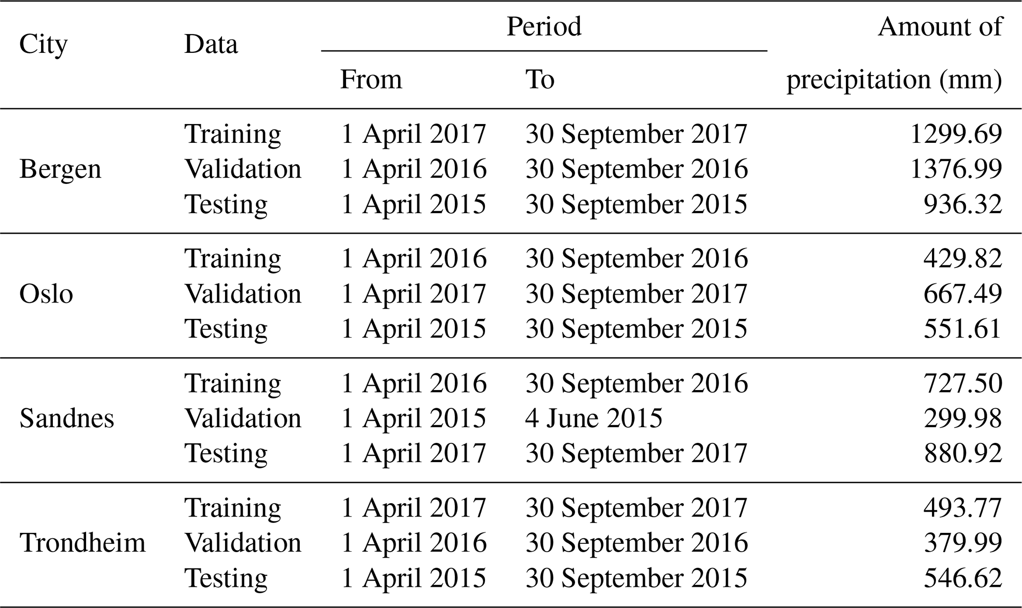
Table 2 Periods selected for model training, validation and testing.

Table 3 Selected ML hyperparameters for tuning.

3.2 ML modelling steps

A general equation was developed relating runoff to climatic variables as follow (Eq. 8):

$$\begin{array}{}\text{(8)}& \begin{array}{rl}{R}_t& =f(P_t,P_{t-\mathrm{1}},P_{t-\mathrm{2}},\mathrm{\dots },P_{t-\mathrm{lag}},{\mathrm{Ta}}_t,{\mathrm{Ta}}_{t-\mathrm{1}},{\mathrm{Ta}}_{t-\mathrm{2}},\\ & \mathrm{\dots },{\mathrm{Ta}}_{t-\mathrm{lag}},W_t,W_{t-\mathrm{1}},W_{t-\mathrm{2}},\mathrm{\dots },W_{t-\mathrm{lag}},{\mathrm{Rh}}_t,\\ & {\mathrm{Rh}}_{t-\mathrm{1}},{\mathrm{Rh}}_{t-\mathrm{2}},\mathrm{\dots },{\mathrm{Rh}}_{t-\mathrm{lag}}).\end{array}\end{array}$$

R is green roof runoff, P is precipitation, Ta is air temperature, W is wind speed and Rh is relative humidity. This is a simplification as the physical properties of the green roof also affect its runoff. However, using data from the same green roofs in this study, Johannessen et al. (2018) found only a small variation in the hydrological performances between the different roof configurations and found the climatic variables to have high impacts on their performance. In the ML models in this study, climatic variables were lagged to represent the initial saturation of the green roofs at each time t. The values of lag were optimized for each green roof and for each ML model during the process of hyperparameters optimization.

Data were aggregated into 1 h resolution, and snow accumulation periods were excluded (1 October–31 March). The data of each green roof were divided into three sets: training, validation and testing. The training datasets were used to train the parameters of the ML models. Validation datasets were used for hyperparameters optimization while the testing datasets were used for the independent evaluations of the ML models and for the comparisons with the conceptual models. The periods between 1 April to 30 November 2015 were used as testing datasets. At Sandnes, only data of 2 months in 2015 are available due to issues with the measurements. Hence, the periods of 1 April to 30 November 2017 were used as testing periods at Sandnes. Initially, the selection of the training periods was based on the amount of precipitation presented in Table 2; the wettest year between 2016 to 2017 were initially selected as training periods. The rationale for the selection was that the wettest year covers a broader span of precipitation events which improves the generalization performance of the models. After the hyperparameters optimization, we further analysed the change of ML performance when using the validations datasets for model training. Some of the validation datasets slightly improved the ML performance and hence were selected as training datasets. The final selection of the training, validation and testing periods is presented in Table 2.

3.2.1 ML hyperparameter tuning

ML models were tuned to achieve good modelling performance and to avoid overfitting. Hyperparameter tuning is the process of finding the optimal ML hyperparameters for the problem (number of hidden layers in ANN, number of LSTM units, k value in kNN, etc.). Bayesian optimization (BO) was selected for hyperparameters tuning (Snoek et al., 2012). This algorithm is suitable for functions in which evaluating one set of parameters is expensive and time-consuming. It was applied by Worland et al. (2018) to optimize hyperparameters for several machine learning models to predict low flows for ungauged basins. In Bayesian optimization, the objective function (i.e. the relation between ML hyperparameters and the performance of the ML model in the validation dataset) is approximated by a probabilistic model (e.g. Gaussian process) that is used to select the most promising hyperparameter to evaluate in the true objective function. The algorithm works as follows:

1. Select initial points of hyperparameters randomly and evaluate them in the true objective function.

2. Build a probabilistic model of the objective function (surrogate function) based on the initial points. The Gaussian process was selected as the surrogate function of the objective function (Snoek et al., 2012; Worland et al., 2018).

3. Choose which hyperparameter to evaluate next in the true objective function based on the surrogate function by optimizing an acquisition function. The expected improvement (EI) was used as an acquisition function in this study (Snoek et al., 2012; Worland et al., 2018).

4. Use the new evaluated point to update the surrogate function.

5. Repeat steps 2–4 for N iterations.

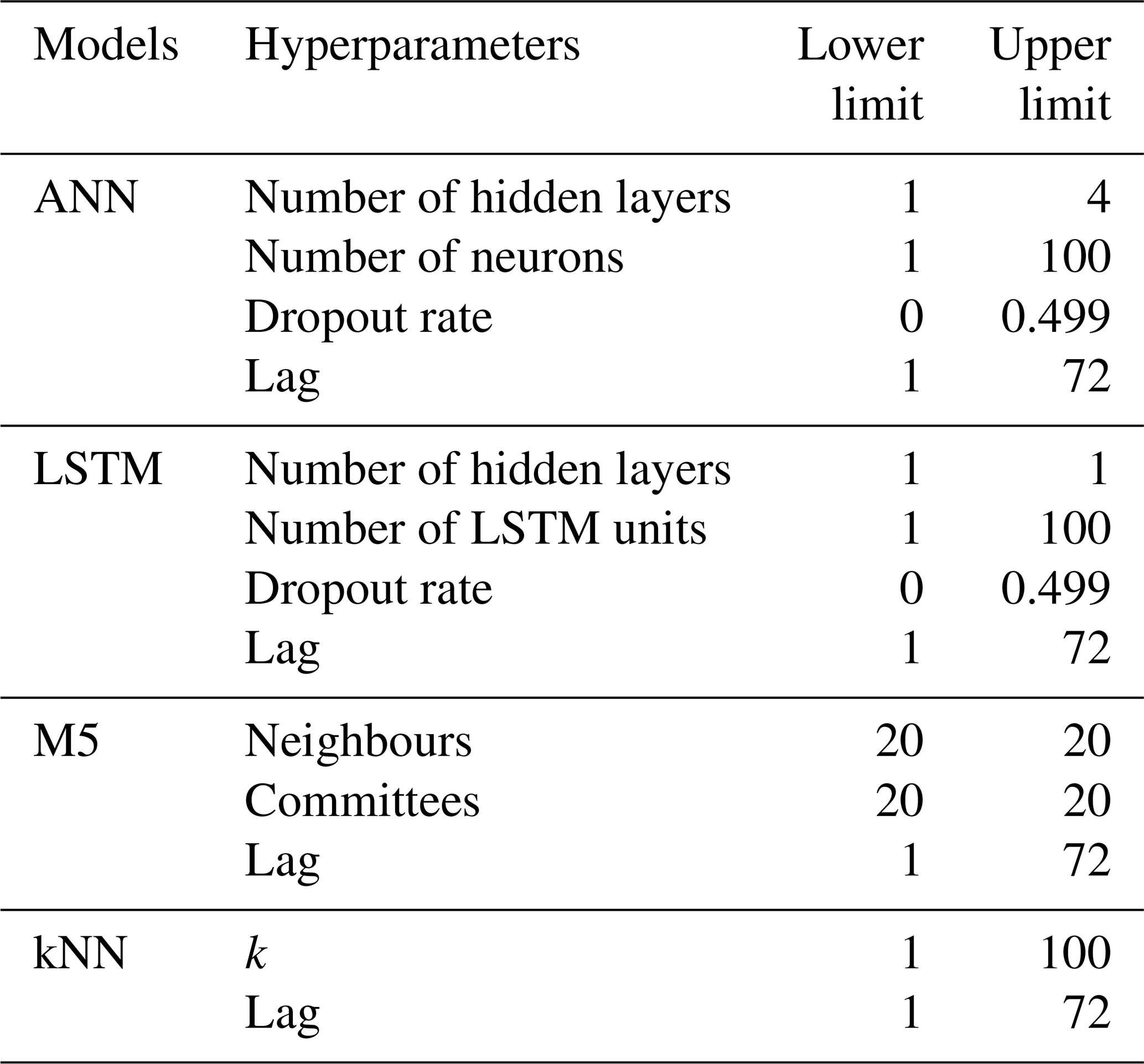
Prior to optimization, ML hyperparameters that require tuning and their upper and lower limits were selected (Table 3), following similar studies (Kratzert et al., 2019; Shortridge et al., 2016). For ANN and LSTM, dropout layers were implemented as a measure to reduce overfitting (Srivastava et al., 2014). At the dropout layer, a specific portion of the optimized weights and biases are set to zero randomly at each training epoch. This technique is used to prevent the network from learning a specific pattern of the input noises and to focus on learning the general patterns of the data. For LSTM, only one hidden layer was selected for this study following the recommendation of the study of Ayzel (2019) in which a grid search was performed for LSTM hyperparameters which compared thousands of LSTM structures. One hidden layer was found to perform reasonably well with lower computational cost compared with multiple hidden layers.

In the first step of the BO, random samples of hyperparameters (five in this study) were drawn from the selected ranges presented in Table 3. These initial points were used to build a Gaussian process model. The Gaussian process model represents the objective function by constructing posteriors distribution of functions with high uncertainty bound far from the sampled points and low uncertainty bounds near the sampled points. In the next step, a continuous function (EI) is calculated for each point x along the Gaussian process model by determining two components. First, how much improvement is expected at x by comparing the mean of the Gaussian process model at the point x with the current best estimate from the sampled points. Second, how much is the uncertainty of the Gaussian process model at the point x, based on the uncertainly bounds. The point x that maximizes the value of EI is selected to be evaluated in the true objective function and the result is used to update the Gaussian process model for the next iteration. At the first iterations, the values of EI function are higher for regions with high uncertainty, so the algorithm fever points in new regions (exploration). After many iterations and new samples, the uncertainty bounds of the Gaussian process model decreases and the algorithm fevers areas with better solutions (exploitation). After N iterations (100 in this study), the algorithm returns the hyperparameters that generate the best solution. In this study, the R library “ParBayesianOptimization” (Wilson, 2021) was used for the BO.

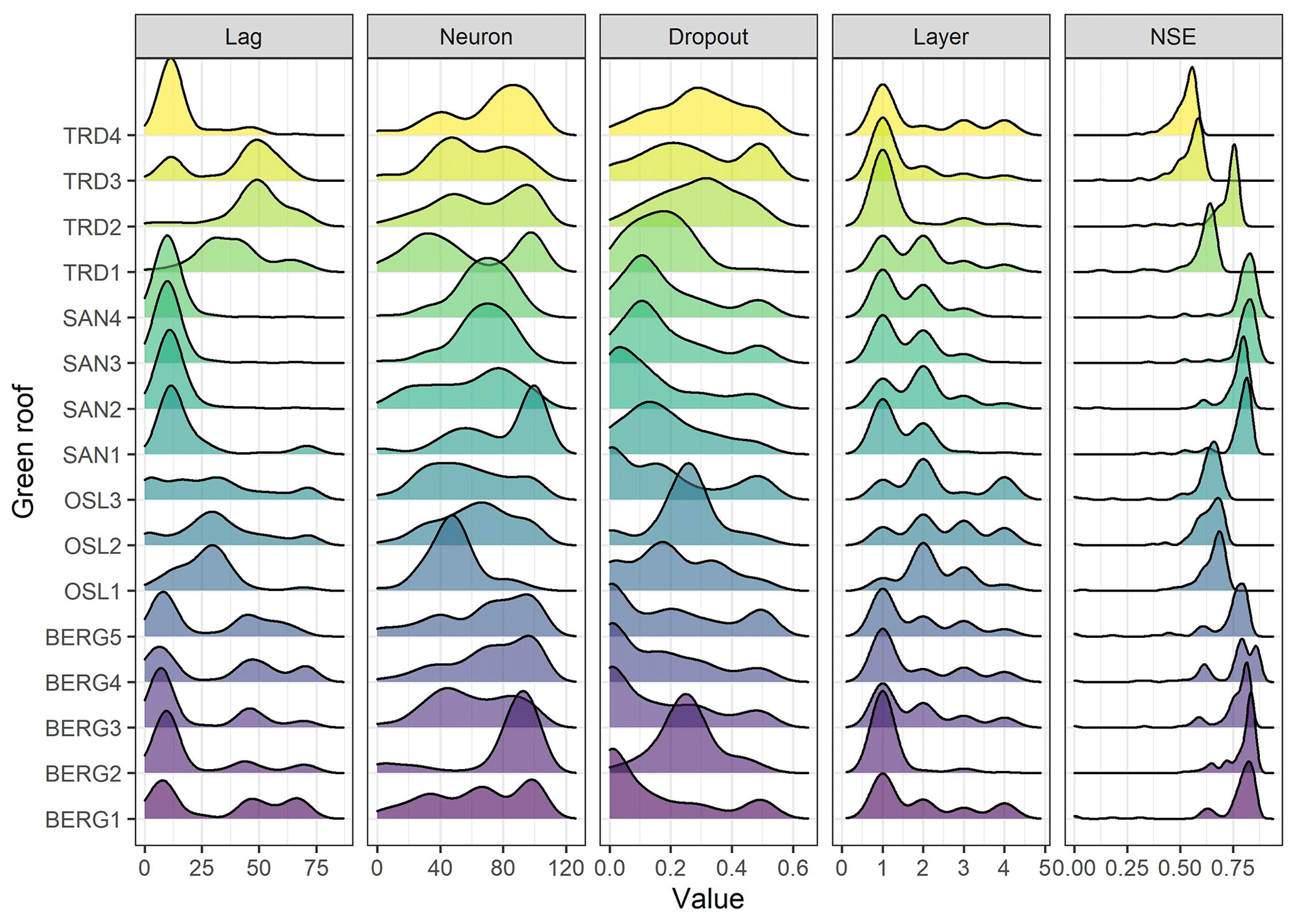
Figure 3 Empirical density distributions of the selected ANN hyperparameters by the Bayesian optimization algorithm and their associated performances in the validation datasets.

Table 4 Results of ML hyperparameter tuning.

Table 5 Overall modelling performance (testing data).

3.3 The conceptual retention model

The 16 roofs were modelled using a conceptual retention model (RM), which was developed and validated by Stovin et al. (2013). The RM model is intended to provide a robust tool that estimates green roof retention using simple water balance equations (Eqs. 9, 10 and 11).

$$\begin{array}{}\text{(9)}& {\displaystyle }{R}_t=max(\mathrm{0},P_t-(S_{\max }-S_t)-{\mathrm{AET}}_t),\text{(10)}& {\displaystyle }{S}_t=\min \mathrm{}(S_{t-\mathrm{1}}+P_t-{\mathrm{AET}}_t,\mathrm{0}),\text{(11)}& {\displaystyle }{\mathrm{AET}}_t={\mathrm{PET}}_t\times {\displaystyle \frac{S_{t-\mathrm{1}}}{S_{\max }}},\end{array}$$

R_t is the runoff from a green roof at time t, P_t is the precipitation at time t, S_max is the maximum storage available in a green roof and S_t is the water stored in a green roof at time t. In our study region, Johannessen et al. (2018) found the Oudin's model for ET to be the most accurate for their water balance model, and Almorox et al. (2015) recommended the use of Oudin for cold climates. Hence, the potential evapotranspiration was computed using Oudin's model as follows (Eqs. 12):

$$\begin{array}{}\text{(12)}& \begin{array}{rl}& \mathrm{PET}\left({\displaystyle \frac{\mathrm{mm}}{\mathrm{day}}}\right)=\\ & \left\{\begin{array}{ll}\mathrm{0},& \text{if}{\mathrm{Ta}}_{\mathrm{mean}}\mathrm{\le }\mathrm{5}{}^{\circ }\mathrm{C};\\ \frac{\mathrm{Ra}}{\mathit{\lambda }\mathit{\rho }}\times \mathrm{0.01}\times ({\mathrm{Ta}}_{\mathrm{mean}}+\mathrm{5}),& \text{if}{\mathrm{Ta}}_{\mathrm{mean}}>\mathrm{5}{}^{\circ }\mathrm{C}.\end{array}\right.\end{array}\end{array}$$

Ta_mean is the daily mean temperature, Ra is extra-terrestrial radiation derived from Julian day and latitude (MJ m⁻²), $\frac{\mathrm{1}}{\mathit{\lambda }\mathit{\rho }}\approx \mathrm{0.408}$, λ is the latent heat of water (MJ kg⁻¹) and ρ is the volumetric mass density of water (kg m⁻³).

The parameter S_max represents the maximum retention capacity of the green roof or the difference between the field capacity and the permanent wilting point of the green roof substrate (Stovin et al., 2013). There exist standard laboratory tests to physically measure the substrate field capacity (Breuning and Yanders, 2008) and the permanent wilting point (Fassman and Simcock, 2012). In this study, however, S_max values were estimated by assuming the field capacities of the roof layers from reported literature values as follow: vegetation mats were assumed to have 20 % of the total substrate depth as a field capacity (Johannessen et al., 2018), brick-based substrates were assumed to have 25 % of the total substrate depth as a field capacity (Stovin et al., 2013) and the drainage mats were assumed to have no permanent storage. The retention models with estimated S_max are referred to as uncalibrated retention models (RM_uncalib).

Figure 4 Comparison between the rainfall events at the four Norwegian cities.

To allow for fair comparison with the ML models, retention models with calibrated S_max values were used (RM_calib). For each roof, we ran the conceptual model by varying the value of S_max between 10 % to 50 % of the substrate total depth. Values of S_max that minimize the Volumetric error of the RM model were selected. The training periods in Table 2 were selected for calibration.

Figure 5 Cumulative precipitation, observed and simulated runoff of the green roofs.

3.4 ML model evaluation

Methods were evaluated based on the performance with the testing datasets. With respect to retention estimation, flow accumulation curves were plotted for the simulated runoff from ML models against the observed runoff and compared with the results from the conceptual retention model. In addition, the percentage bias (PBIAS) values (Eq. 13) were calculated for each simulation for comparison. To evaluate the performance of ML models in estimating the temporal variation in runoff, the simulated runoff from ML models were plotted against the observed values and the NSE (Eq. 14) values were determined. Values of NSE >0.5 were considered satisfactory (Moriasi et al., 2007; Rosa et al., 2015). To evaluate the potential of using ML as a useful tool for planning and design purposes, ML models were transferred between the roofs unchanged. The transferred models simulated the testing periods of each roof, and NSE was used to evaluate the transferability performance. Moreover, a volumetric factor (vol) based on the PBIAS was determined by using Eq. (15) to assess transferability in terms of volume estimation. A vol value of 1 indicates a perfect runoff volume estimation and hence a perfect retention estimation, while a vol value of 0 indicates 100 % error in volume estimation. Additionally, we compared the performance of transferred ML models with the uncalibrated retention models.

$$\begin{array}{}\text{(13)}& {\displaystyle }\mathrm{PBIAS}=\mathrm{100}\times {\displaystyle \frac{\sum Q_{\mathrm{obs}}-\sum Q_{\mathrm{sim}}}{\sum Q_{\mathrm{obs}}}},\text{(14)}& {\displaystyle }\mathrm{NSE}=\mathrm{1}-{\displaystyle \frac{\sum (Q_{\mathrm{obs}}-Q_{\mathrm{sim}}{)}^{\mathrm{2}}}{\sum (Q_{\mathrm{obs}}-\stackrel{\mathrm{‾}}{Q_{\mathrm{obs}}}{)}^{\mathrm{2}}}},\text{(15)}& {\displaystyle }\mathrm{vol}=\mathrm{1}-{\displaystyle \frac{\left|\mathrm{PBIAS}\right|}{\mathrm{100}}}.\end{array}$$

4 Results and discussion

4.1 Hyperparameter optimization (model tuning)

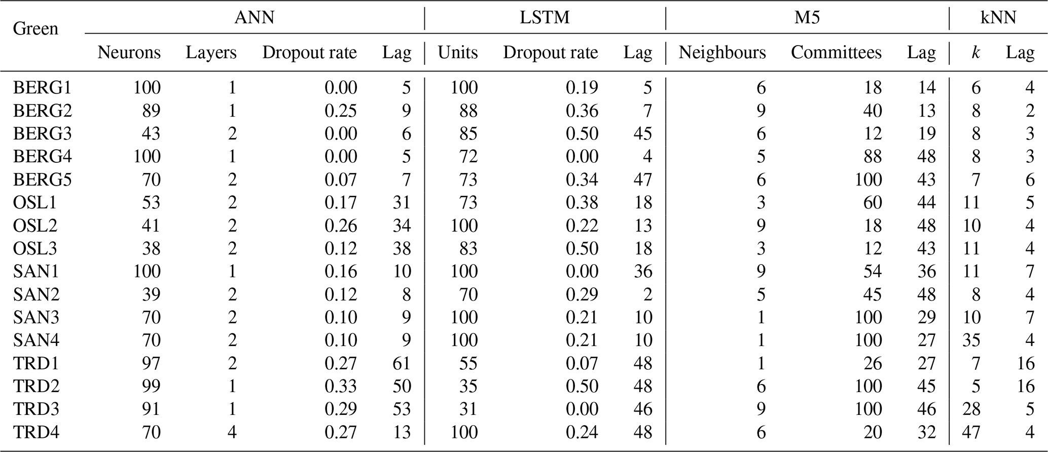
For LSTM and ANN models, the number of epochs was selected prior to the BO process by running an initial ANN model with 1000 epochs. After 30 epochs, the performance in the validation data did not improve further and started to decrease after 100 epochs while improving in the training dataset, which indicates overfitting. Therefore, 30 epochs were selected as an optimal value. Then, the BO algorithm was applied with 100 iterations for each ML model and for each roof. The selected hyperparameters of each iteration were stored. Figure 3 presents the empirical probability density distributions of the selected ANN hyperparameters by the BO and their associated performances in the validation datasets. The results can interpreted as that hyperparameters with high density values are located in regions that maximized the modelling performance in the validation datasets. The hyperparameters that generated the best results at the validation datasets were selected for each roof and each ML model, as presented in Table 4.

Based on Fig. 3, ANN with one hidden layer was found to be sufficient for most of the roofs in the study. Hence, deep ANN architectures, i.e. ANN models with many hidden layers, might not be required for this task. This has an important implication as deep ANN models are computationally expensive and prone to overfitting. Likewise, Ayzel (2019) found that deep LSTM models are not required for predicting runoff at hourly time steps, while Zhang et al. (2018) found a single-layer LSTM to perform better than an LSTM model with two layers for predicting daily water level depths in agricultural land.

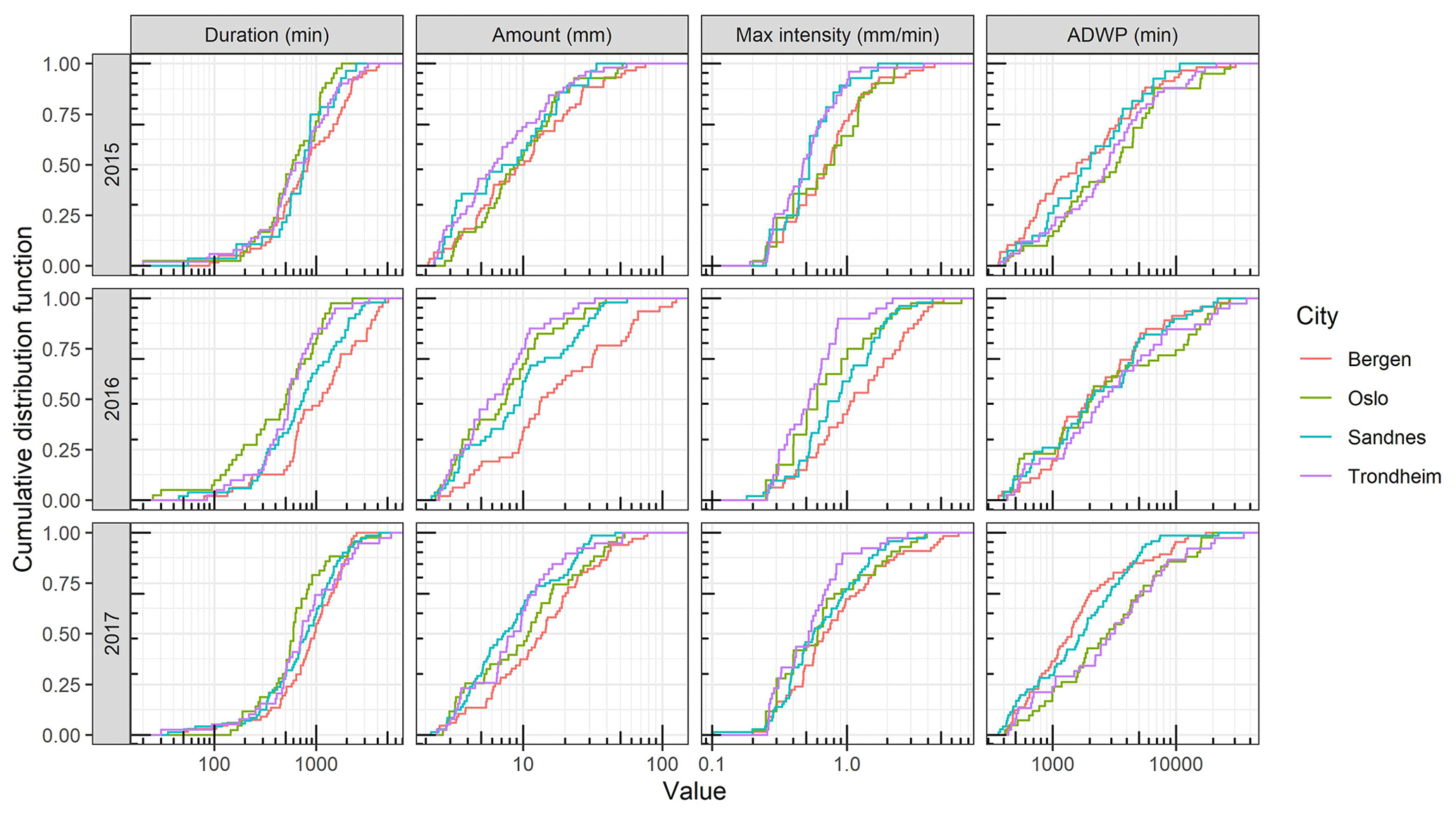
Another interesting finding is the lag values which are varied between the cities. It can be noted that the lag values were smaller in Bergen and Sandnes compared to Trondheim and Oslo. To interpret this finding, rainfall events, with 6 h intra-event periods, were extracted from the three datasets at the four cities and compared, as shown in Fig. 4. Bergen roofs received events with higher amount and duration compared to Oslo and Trondheim roofs, whereas the antecedent dry weather periods (ADWPs) at Oslo and Trondheim are longer than BERG. Hence, due to the longer ADWP, a longer memory of the system is required to account for the wider range of possible initial saturation, compared to Bergen roofs.

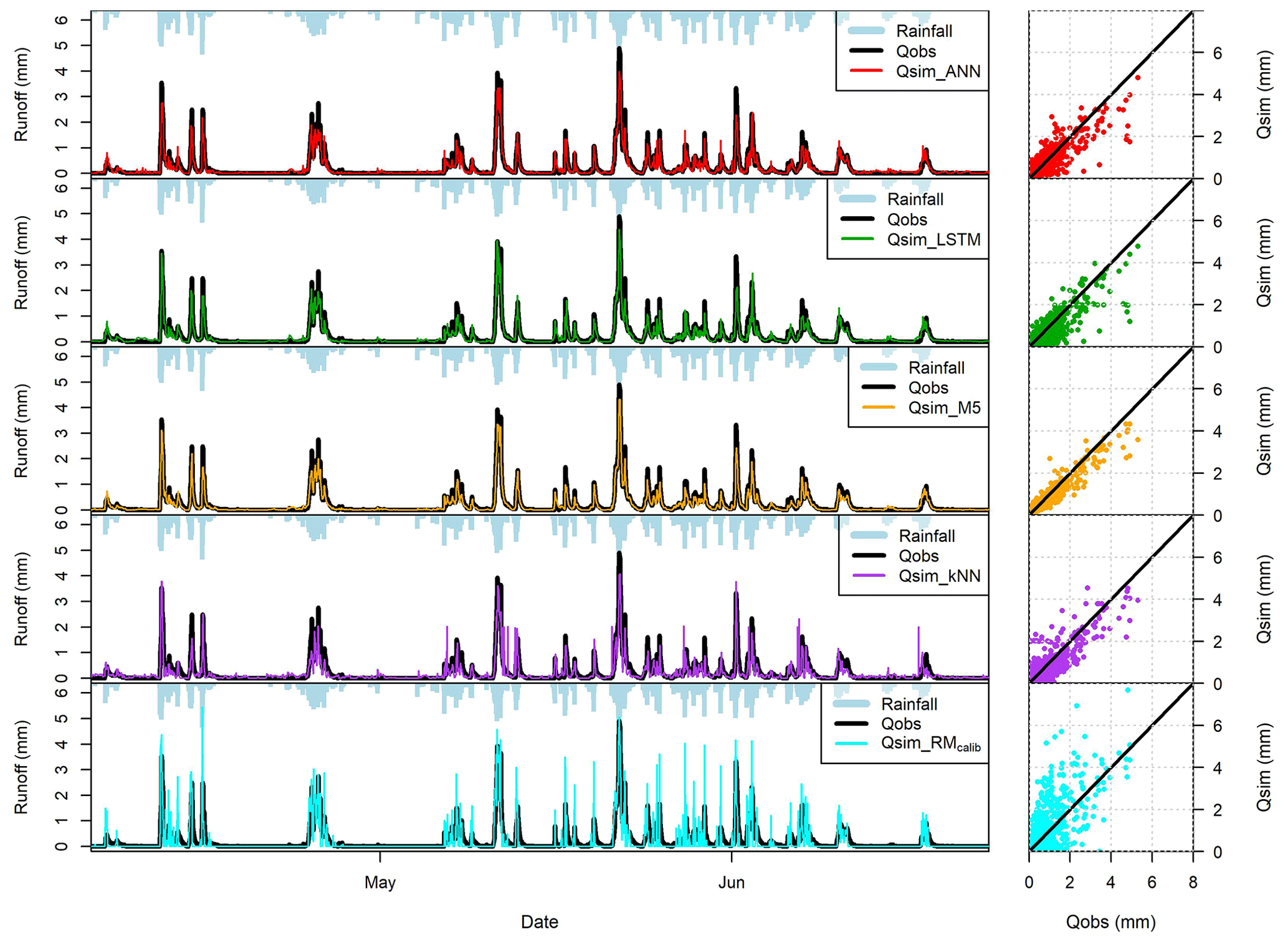
Figure 6 Performance of ML models on the testing period (BERG 2). The hydrographs were plotted for around 3-month period (2000 h), while the Q–Q plots were plotted for the entire testing period.

Figure 7 Comparison between LSTM and ANN at TRD1 roof.

4.2 Model evaluations

4.2.1 Retention estimation

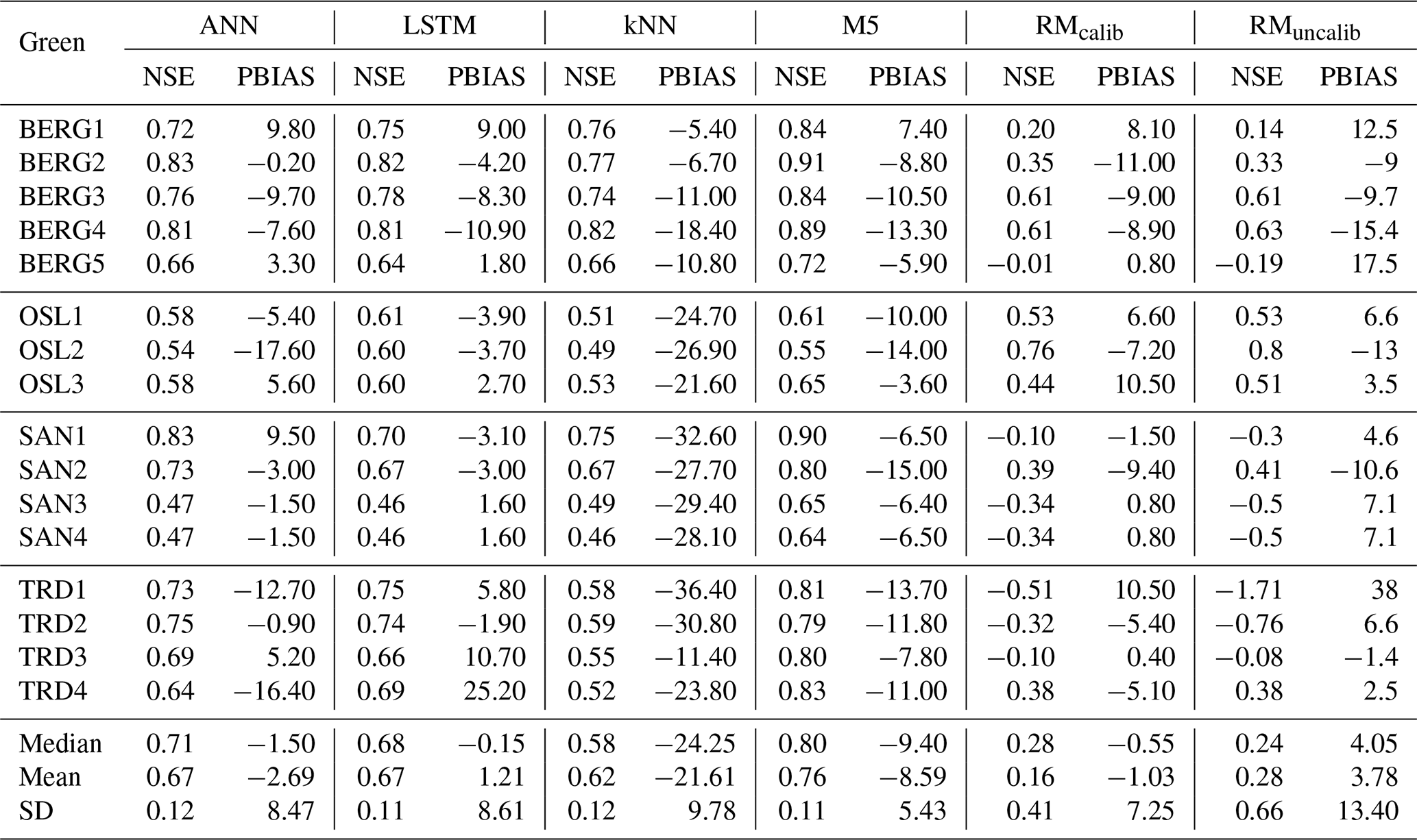
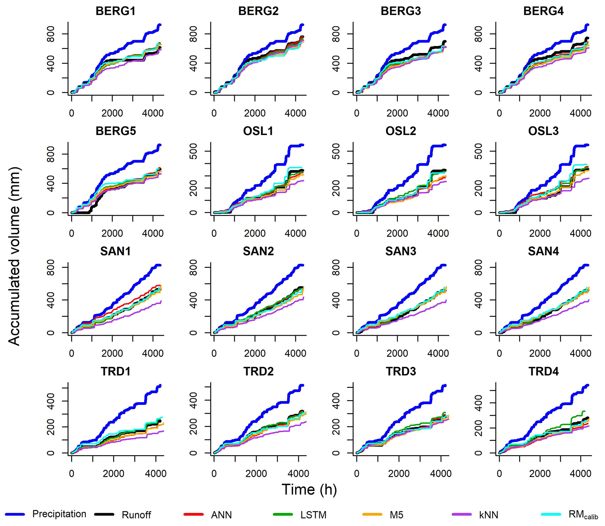
Machine learning models were built for all roofs based on the optimized hyperparameters, which were selected by the BO algorithm. Figure 5 illustrates the simulated and observed runoff cumulative curves together with the cumulative precipitation for each roof, and Table 5 shows the values of PBIAS and NSE of the models at the testing datasets. The results presented in Fig. 5 and Table 5 confirm that the ML models and the conceptual models can reproduce the observed runoff volume in most of the green roofs. By comparing the median values of the PBIAS on the testing periods, LSTM yielded only −0.15 % with a standard deviation of 8.61 %. Following LSTM, median values of −0.55 %, −1.50 % and 4.05 % were obtained by the RM_calib, ANN and RM_uncalib models, respectively. The M5 models yielded simulation with a median PBIAS of −9.4 % while the kNN yielded the highest volumetric errors with a median PBIAS of −24.25 % with a standard deviation of 9.78 %. It can be noted that the conceptual retention models and ML models, except kNN, could produce results that are classified as acceptable modelling results regarding volumetric error (|PBIAS| < 25 %), as per Moriasi et al. (2007).

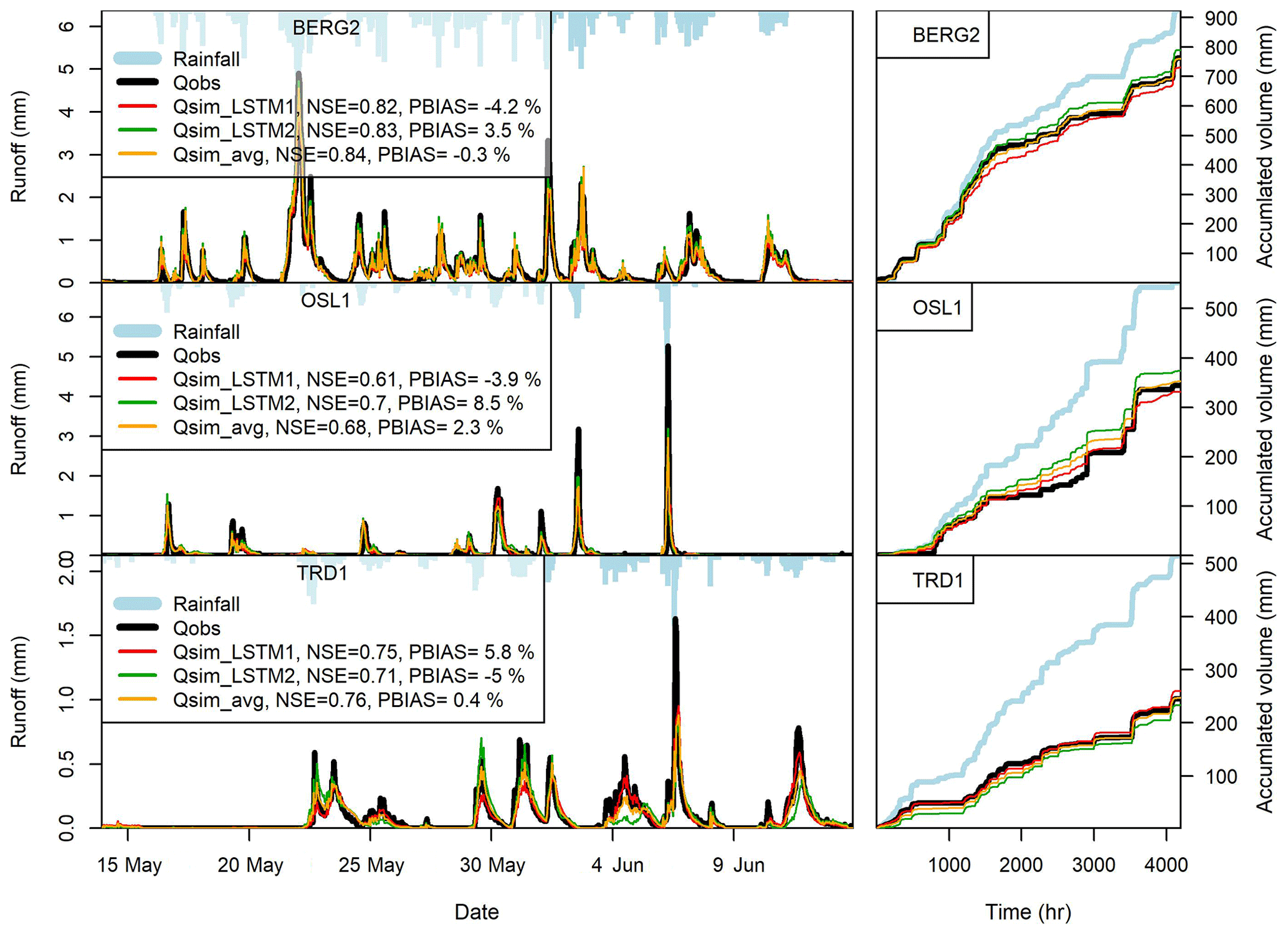
Figure 8 The performance of LSTM models in the testing datasets at BERG2, OSL1 and TRD1 roofs when using different data for model training. LSTM1 is trained using the testing period presented in Table 2, while LSTM2 is trained using the validation period presented in Table 2. Qsim-avg is the average of Qsim-LSTM1 and Qsim-LSTM2.

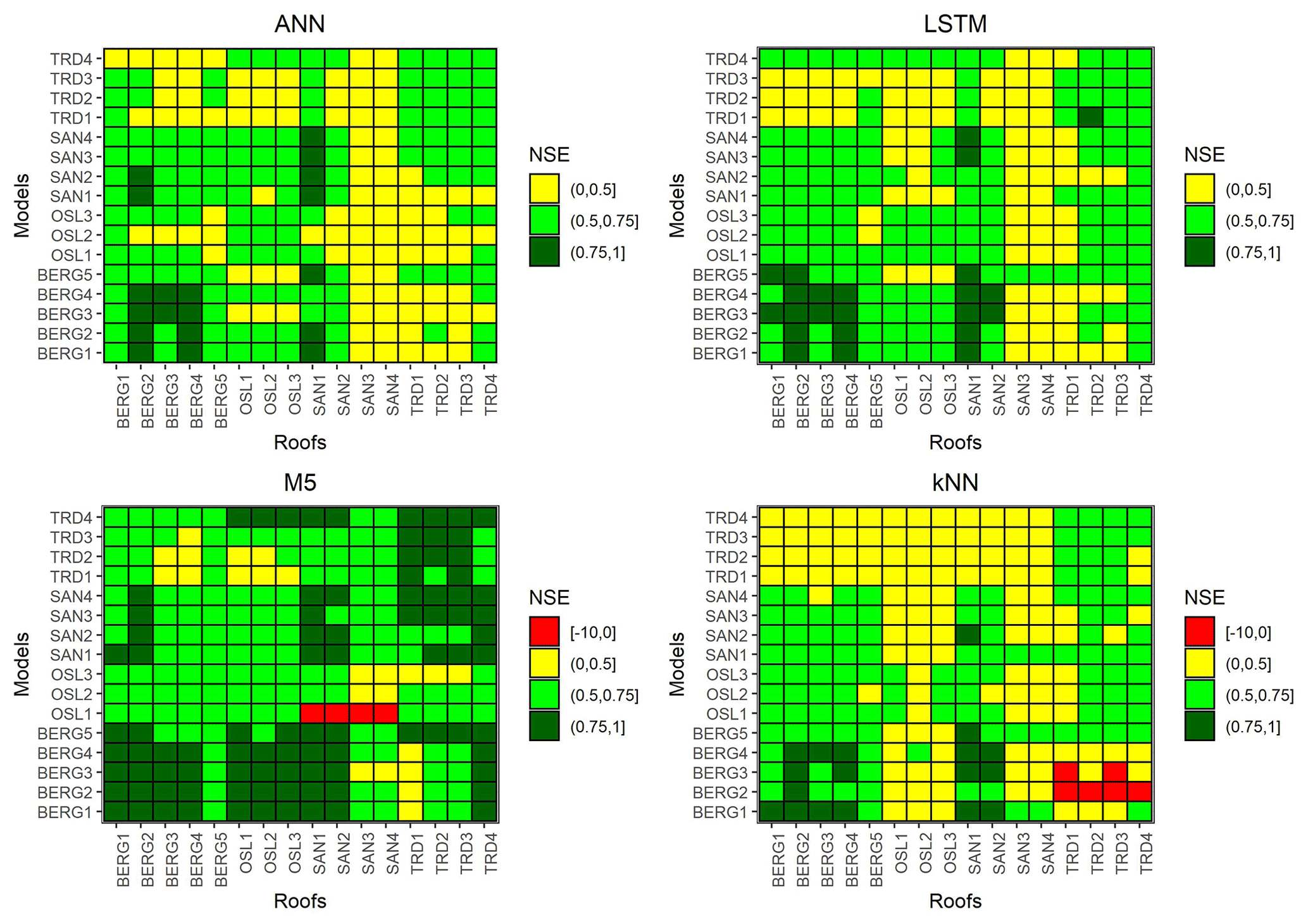
Figure 9 Transferability between the different roofs (NSE). Models on the y axis are used to simulate the measured green roofs on the x axis.

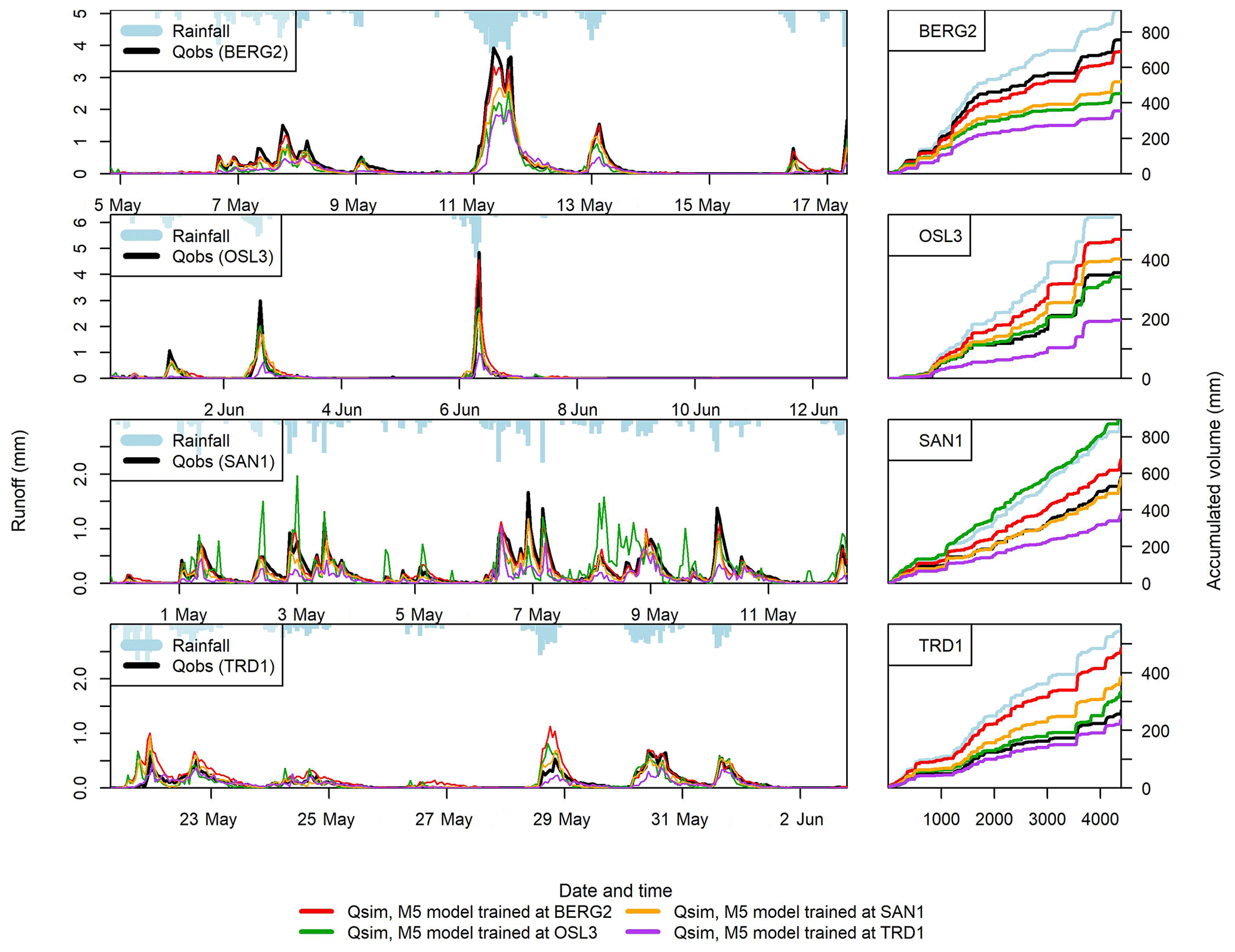
Figure 10 The performance of the transferred ML models at BERG2, OSL3, SAN1 and TRD1. The hydrographs were plotted for selected periods, while the cumulative plots were plotted for the entire testing period.

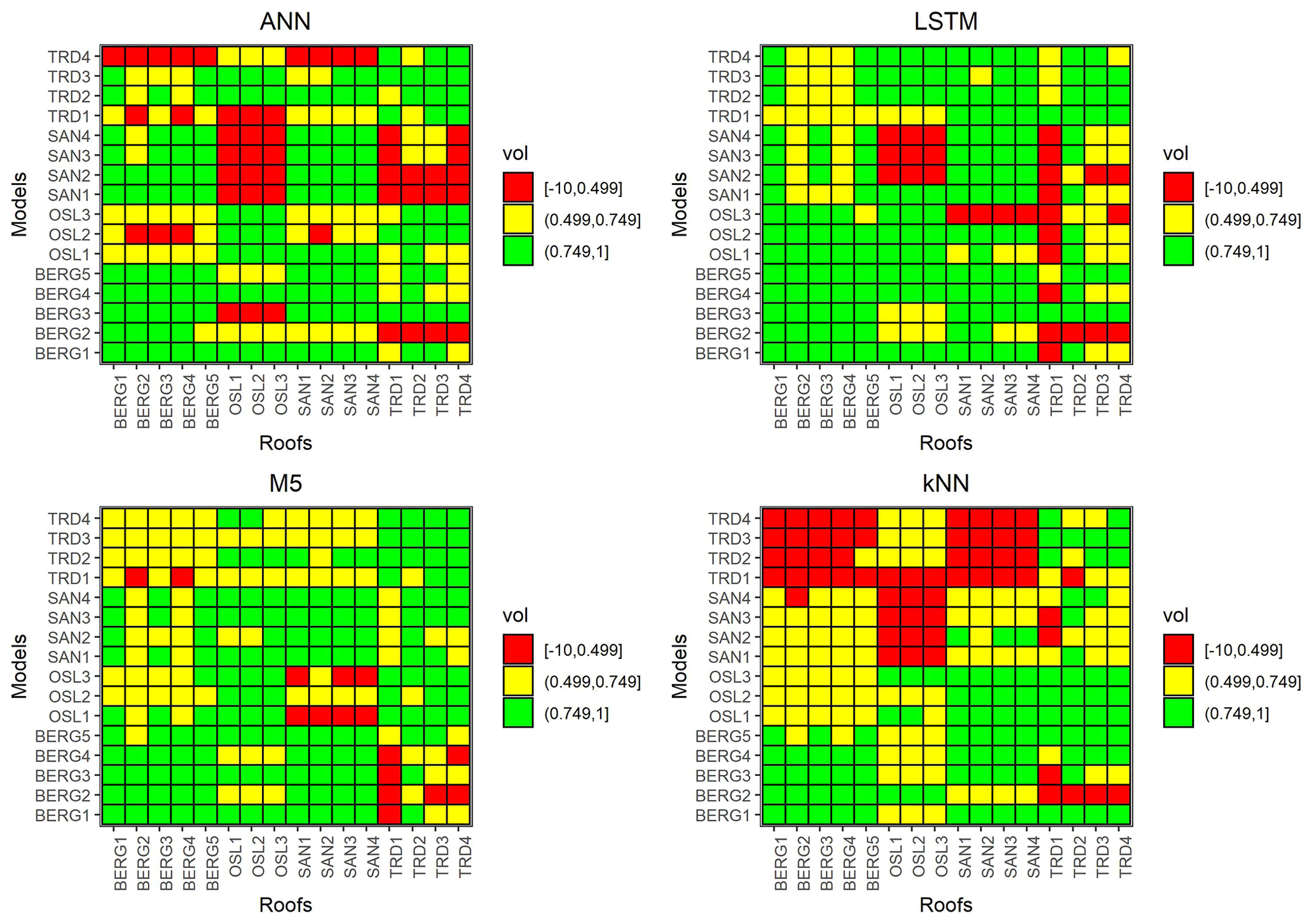
Figure 11 Transferability between the different roofs (vol). Models on the y axis are used to simulate the measured green roofs on the x axis.

4.2.2 Temporal variations in runoff

Table 5 presents the NSE values for training and validation periods for the ML models. Most ML models yielded satisfactory results in the testing periods (NSE > 0.5). M5 models produced results with highest NSE values, with a median value of 0.80. Both ANN and LSTM produced result with a median NSE values of 0.67. Figure 6 shows the observed and simulated hydrographs for BERG2 roof, which confirms the ability of the ML models to reproduce the observed runoff. In contrast, the conceptual models produced satisfactory results in only five roofs. We found the green roofs in our study to detain small- and medium-sized events for up to 2 h. The conceptual model failed to simulate these dynamics due to a lack of routing.

The performance of ML models varied between the different cities more than between the different configurations. Johannessen et al. (2018), using the same data in this study, observed similar hydrological performance for the different configuration within the same city. However, it should be noted that the geometries of the roofs are identical at each city (Table 1). The performance of the ML methods can be explained based on this comparison between the cities’ rainfall characteristics (Fig. 4). For instance, the NSE values of the ML models are higher in Bergen roofs in comparisons to Oslo roofs. As mentioned earlier, Oslo roofs have a wider range of possible initial saturations. Therefore, 1 year of training data might not be enough to cover this wide range of runoff possibilities. On the other hand, Bergen roofs received more frequent and intense precipitation events resulting in a small range of possibilities of initial saturation that could be covered using 1 year only. The kNN method produced lower NSE values compared to the other ML models. This was attributed to the relatively small training data used in this study as kNN estimates the performance depending on the similarity to the previous time steps.

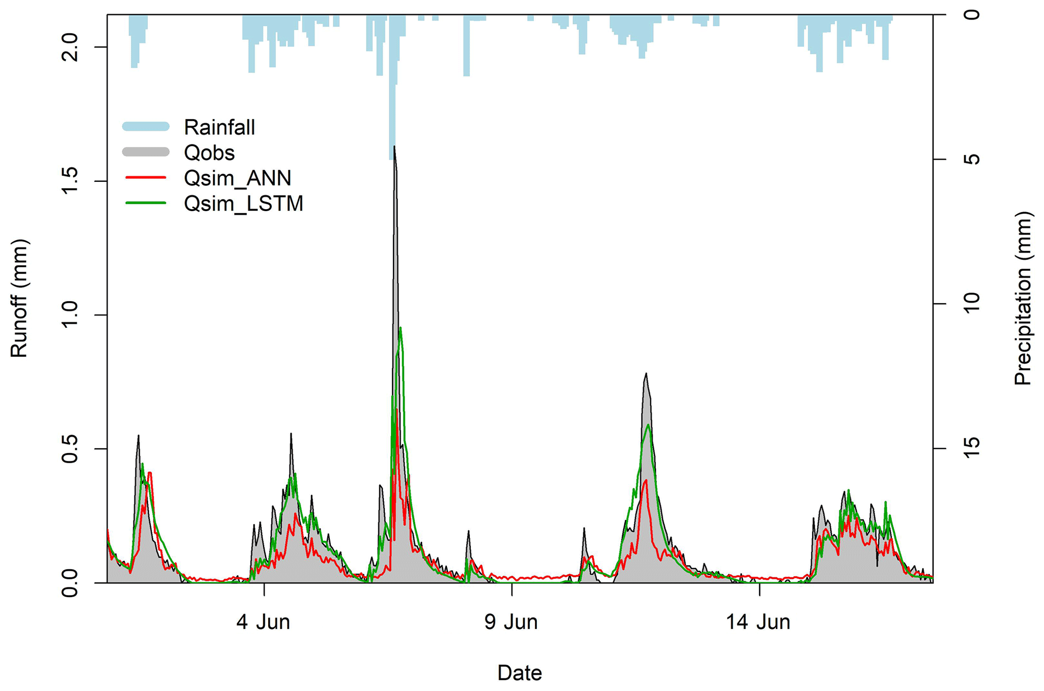
LSTM maintains a state value between consecutive time steps which makes it more suitable for modelling green roofs where initial saturation plays an important role in green roof runoff generation process. A comparison was made between ANN and LSTM at TRD1 (Fig. 7) to demonstrate the potential of LSTM. ANN was found to produce runoff when no precipitation occurred, unlike LSTM. Moreover, LSTM could simulate the flow peaks more accurately than ANN. Likewise, Kratzert et al. (2018) found LSTM simulations to be smoother than a normal recurrent neural network and to be better in accounting for the storage capacity (including snow accumulation) of a natural catchment

4.2.3 Effect of training data and ensemble modelling

The performance of ML models when using different data for model training was evaluated. For each roof, two ML models were built; one by using the training datasets in Table 2 for model training and one by using the validation datasets in Table 2 for model training. Sandnes roofs were excluded from this analysis due the missing data in one 2015, as discussed earlier. Figure 8 demonstrates the performance of LSTM models at BERG2, OSL1 and TRD1 roofs when using different data for model training. The performances of the two LSTM models (LSTM1 and LSTM2) were quite similar, as presented in Fig. 8. One idea that could improve the estimates of the ML models is to combine the simulations from several ML models that are build from different datasets (ensemble modelling). As shown in Fig. 8, the average simulations of two LSTM models yielded better simulation for the testing dataset (lower PBIAS and slightly higher NSE values) in comparison to the estimate of each of the two LSTM models. However, this is only true when the two LSTM models have positive and negative biases. Nevertheless, we found few green roofs where the two LSTM models from the 2 years resulted in biases of the same direction (at BERG3 and OSL3 roofs).

4.2.4 Transferability

Models were transferred between the roofs unchanged to simulate the testing periods. Figure 9 presents the transferability performance measured by NSE. Some models could yield satisfactory results in different locations (NSE >0.5). For instance, M5 models that were trained using data from Bergen roofs could yield satisfactory performance in almost all cities. Figure 10 presents an example of transferred M5 models between BERG2, OSL3,SAN1 and TRD1 roofs. It can be noted that models that are trained in wetter cities, such as Bergen, overestimated the flows at cities with lower precipitation, such as Trondheim. Figure 11 presents the transferability performance with respect to retention estimation measured by vol. Transferred ML model could simulate result with acceptable accuracy (vol >0.75) (Moriasi et al., 2007) between Trondheim and Oslo cities and between Sandnes and Bergen cities with some exceptions. This can be somewhat attributed to the similarity in climatic conditions between the cities (Fig. 4). However, the uncalibrated conceptual models in this study could produce better volume estimates than the transferred ML models in most cases. This implies that using the conceptual model with literature estimates of the S_max parameter is preferable over the transferred ML to estimate the annual retention for new roofs.

4.3 Machine learning potentials for green roof hydrological modelling

The present paper has demonstrated that well-trained ML models can be applied to estimate retention process (rainfall losses) in a range of different green roof systems. The predictions are comparable in accuracy to a conceptual water balance model based on losses due to evapotranspiration. Additionally, well-trained ML models showed more accurate predictions of runoff hydrographs than the conceptual water balance model, which is encouraging for detention modelling. Moreover, aggregating the simulations of many ML models (ensemble modelling) appears to improve the prediction and can be investigated in future studies. Detention modelling is required to estimate the lag and attenuation of runoff associated with any rainfall that is not retained. In practice, many modelling frameworks rely on calibrated reservoir routing models to estimate the cumulative detention effects of multiple interacting component layers, and few (if any) convincing validation cases for a complete detention modelling framework have been presented. It would therefore be very valuable to explore whether the ML models, when trained on higher temporal resolution datasets, have the capability to capture these complex detention effects better than the alternative black-box approaches.

5 Conclusions

Four machine learning models, commonly used in runoff modelling studies, were applied to simulate runoff from 16 green roofs located in four Norwegian cities with different climatic conditions. We further investigated the potential of using ML models to estimate performance of new roofs where runoff data are not available for model training. This was done by means of transferring ML models between the roofs in the study. Our results confirm the ability of well-trained ML models to estimate green roof retention and the temporal runoff dynamics. The estimates of the annual retention were comparable to a proven conceptual model. Despite the 1 h time step, the ML models provided accurate simulations of runoff dynamics, i.e. discharge hydrographs (NSE values higher than 0.5 in most cases), which is encouraging for detention modelling. The LSTM demonstrated better modelling performance by maintaining a state value between consecutive time step, which makes it more appropriate for simulating runoff of green roofs. In future studies, shorter time steps will be applied to estimate detention metrics.

Some transferred ML models could give acceptable model performance (NSE >0.5, |PBIAS| <25 %) in different locations. However, we recommend using the conceptual model with literature values of the S_max parameter to estimate the annual retention of new roofs over the transferred model as it give accurate volume estimations.