Feedback mechanisms between precipitation and dissolution reactions across randomly heterogeneous conductivity fields

Our study investigates interplays between dissolution, precipitation, and transport processes taking place across randomly heterogeneous conductivity domains and the ensuing spatial distribution of preferential pathways. We do so by relying on a collection of computational analyses of reactive transport performed in two-dimensional systems where the (natural) logarithm of conductivity is characterized by various degrees of spatial heterogeneity. Our results document that precipitation and dissolution jointly take place in the system, with the latter mainly occurring along preferential flow paths associated with the conductivity field and the former being observed at locations close to and clearly separated from these. High conductivity values associated with the preferential flow paths tend to further increase in time, giving rise to a self-sustained feedback between transport and reaction processes. The clear separation between regions where dissolution or precipitation takes place is imprinted onto the sample distributions of conductivity which tend to become visibly left skewed with time (with the appearance of a bimodal behavior at some times). The link between conductivity changes and reaction-driven processes promotes the emergence of non-Fickian effective transport features. The latter can be captured through a continuous-time random-walk model where solute travel times are approximated with a truncated power law probability distribution. The parameters of such a model shift towards values associated with increasingly high non-Fickian effective transport behavior as time progresses.

1 Introduction

Diagnosis and characterization of the feedback between geochemical precipitation/dissolution reactions and solute transport processes in heterogeneous subsurface systems is key to a variety of environmental and Earth science scenarios (Rege and Fogler, 1989; Berkowitz et al., 2016). A critical challenge is the emergence of complex dependencies between physical and chemical processes taking place across aquifer bodies (Saripalli et al., 2001). Heterogeneity of these systems promotes diverse patterns of precipitation and/or dissolution that may imprint a variety of dynamic system responses, including, for example, wormhole and oscillatory behaviors of system attributes such as porosity and permeability (Edery et al., 2011; Garing et al., 2015; Golfier et al., 2002). Examples of practical applications in this context include geologic CO₂ storage (e.g., Pawar et al., 2015; Noiriel and Daval, 2017; Cabeza et al., 2020, and references therein), acid injection in production wells (e.g., Liu et al., 2017, and references therein), and reactive transport of contaminants (e.g., Ceriotti et al., 2018; Dalla Libera et al., 2020, and references therein).

Computational studies can assist the analysis of patterns of chemical transport across heterogeneous subsurface systems in the presence of precipitation/dissolution phenomena. While requiring an explicit description of the spatial heterogeneity of the system properties (Atchley et al., 2014), routine application of numerical simulations in practical settings is hampered by (i) our limited knowledge of the system attributes, resulting in uncertainty affecting the parameterization of the underlying physical and chemical processes and their variability, and (ii) the computational costs required to properly quantify such uncertainties and their propagation onto environmental quantities of interest. In this context, we rely on an effective approach to characterize the evolution of key features of solute transport in the presence of rock–fluid interactions across a porous medium whose spatially heterogeneous conductivity field is interpreted according to a commonly employed stochastic framework.

A critical element we tackle is related to the analysis of the dynamic feedback between reactive transport and spatially heterogeneous distributions of porous media attributes such as hydraulic conductivity. Following prior studies, we start by recognizing that, even under geochemical equilibrium conditions, the spatial heterogeneity of system attributes typically imprints an uneven spatial distribution of regions where chemical reactions take place, local fluctuations of conductivity being key to this element (Edery et al., 2016a). Further to this, our conceptualization of the setting is grounded on the observation that rendering of transport features in geological formations through effective formulations typically requires embedding non-Fickian features. To this end, we rely on an upscaled description of transport where solute travel/waiting times are approximated with a truncated power law probability density function (PDF), hereafter termed TPL (Berkowitz et al., 2006). This effective description is particularly relevant, because the emergence of non-Fickian transport features in heterogeneous formations has been observed at diverse scales of observation, including pore-, laboratory- and field-scale scenarios (e.g., Edery et al., 2011; Muljadi et al., 2018; Menke et al., 2018, and references therein).

In line with our objective, we rest on the framework of analysis developed in Edery et al. (2014, 2016a), where an effective depiction of transport processes is parameterized as a function of the statistics of solute residence times in randomly heterogeneous conductivity fields. A main element of this framework is that it yields a link between the TPL weighting times and the occurrence of preferential pathways that can be obtained from computational studies of transport in such conductivity fields (Edery et al., 2014). As a result, the methodology is conducive to an effective (or upscaled) representation of local features to identify signatures of non-Fickian transport (see also Dentz et al., 2011; Edery et al., 2014). To illustrate the main features associated with the scenario of interest, we consider a Darcy-scale formulation of a reactive transport setup, where precipitation and/or dissolution of minerals are driven by the injection of an acid compound establishing local equilibrium with the resident fluid and a solid matrix of the host porous medium which is considered to be composed of calcite mineral. While the geochemical processes we consider are somehow streamlined with respect to a field-scale scenario (see, for example, Lichtner, 1988; Dreybrodt et al., 1996), they embed the main elements characterizing the interplay between solute transport and rock–fluid interactions in Darcy-scale systems (e.g., Edery et al., 2011). Within this conceptual picture, our study aims at investigating (i) the interplay between the reactive process and the ensuing spatial distribution of preferential pathways associated with spatially heterogeneous conductivities and (ii) the link between locally occurring reaction-driven phenomena and emerging non-Fickian effective transport features, as captured by the TPL formulation of the PDF of particle travel/waiting times.

2 Methodology

2.1 Chemical model

We simulate a reactive transport scenario where calcite (CaCO_3(s), subscript (s) denoting solid mineral) can dissolve or precipitate locally in the presence of chemical equilibrium between dissolved carbonic acid (H₂CO₃) and pH. The amount of dissolved H₂CO₃ as a function of pH (see Fig. S1 in the Supplement) is then governed by equilibrium conditions, which is tantamount to assuming a locally instantaneous reaction (i.e., as the reactive timescale approaches zero at equilibrium, this scenario corresponds to a local Damköhler number which tends to infinity). The formulation describing the chemical reactions can then be streamlined as

$$\begin{array}{}\text{(1a)}& {\displaystyle }{\mathrm{CaCO}}_{\mathrm{3}\left(\mathrm{s}\right)}\leftrightarrow {\mathrm{Ca}}^{\mathrm{2}+}+{\mathrm{CO}}_{\mathrm{3}}^{\mathrm{2}-},\text{(1b)}& {\displaystyle }{\mathrm{H}}_{\mathrm{2}}{\mathrm{CO}}_{\mathrm{3}}\leftrightarrow \mathrm{2}{\mathrm{H}}^{+}+{\mathrm{CO}}_{\mathrm{3}}^{\mathrm{2}-},\end{array}$$

according to which two protons (H⁺) in Eq. (1b) react with ${\mathrm{CO}}_{\mathrm{3}}^{\mathrm{2}-}$ to produce H₂CO₃ that in turn drives dissolution of the host calcium carbonate solid matrix. While simplified (see, for example, Lichtner, 1988; Dreybrodt et al., 1996), the chemical setup follows previous work by Edery et al. (2011), where there is an extensive assessment of the employed formulation (see also the Supplement). In this context and consistent with typical experimental practice, we consider the injected fluid and the porous medium to be associated with a source of H⁺ and an abundance of Ca²⁺, respectively. Thus, Ca²⁺ is not rate-limiting, and the spatial distribution of H⁺, as driven by transport and reaction, governs pH. The rate-limiting reaction is then Eq. (1b), that is controlled by the available H⁺ (or pH), similar to observations associated with other studies (Singurindy and Berkowitz, 2004; Edery et al., 2011). The chemical reaction system (Eqs. 1a and 1b) is here simplified (see, for example, Krauskopf and Bird, 1967) through

$$\begin{array}{}\text{(2)}& \text{co}\leftrightarrow \mathrm{2}h+c,\end{array}$$

where co denotes H₂CO₃, and h and c represent H⁺ and CaCO_3(s), respectively.

2.2 Flow and transport modeling

Our computational setting is intended to mimic a laboratory-scale scenario where a 60 cm × 24 cm two-dimensional flow cell is filled with a porous system formed by a CaCO_3(s) solid matrix. The system is initially fully saturated with water, and an injection of low-pH water takes place across the upstream side of the cell. To investigate the influence of the dissolution/precipitation reaction on solute transport, we consider a groundwater flow which is uniform in the mean, taking place within a two-dimensional domain where the (natural) logarithm of conductivity, y=ln (k), is considered a zero-mean, second-order stationary random field. The latter is further characterized by an isotropic, simple exponential, covariance function, with (normalized) correlation length $l/L$, with L being the length of the domain along the main flow direction. Various degrees of heterogeneity of the system are analyzed upon considering values of log-conductivity variance ${\mathit{\sigma }}_{\mathrm{0}}^{\mathrm{2}}=[\mathrm{1},\mathrm{3},\mathrm{5}]$, with subscript 0 denoting that these values refer to the initially generated conductivity distributions (i.e., prior to the occurrence of reactions). The domain is discretized through 300 × 120 elements of uniform size Δ = 0.2 cm, yielding a field size of 60 cm × 24 cm. Each field is synthetically generated through the widely tested sequential Gaussian simulator GCOSIM3D (Gómez-Hernández and Journel, 1993) and is characterized by $l/L$ = 0.016. This yields a value of $\mathrm{\Delta }/l$ = 0.2, which is deemed adequate to capture the local features of the covariance of y  and their impact on the main statistics of the velocity field and travel times (Ababou et al., 1989; Riva et al., 2009). We note that, while our study is representative of a laboratory-scale analysis, the dimensions of the domain have no particular implication, and they are only selected to ensure a meaningful description of the correlation structure that is included in the initially generated conductivity fields.

For each value of ${\mathit{\sigma }}_{\mathrm{0}}^{\mathrm{2}}$, 20 random realizations of y are generated, each being then subject to a deterministic pressure drop (ΔH = 100 cm) between the inlet (left) and the outlet (right) sides. The local distribution of fluid velocity is computed through

$$\begin{array}{}\text{(3)}& \mathrm{\nabla }\cdot \mathit{q}\left(\mathit{x}\right)=\mathrm{0},\mathit{q}\left(\mathit{x}\right)=-k\left(\mathit{x}\right)\cdot \mathrm{\nabla }h\left(\mathit{x}\right);\end{array}$$

where q(x) is the local Darcy flux, and vector x corresponding to spatial location. The local fluid velocity field is then obtained as $\mathit{v}=\mathbf{q}/\mathit{\theta }$, with a constant initial porosity θ = 0.4 being here considered for the porous medium.

Solute transport is then simulated across each conductivity field by a particle-tracking approach (Le Borgne et al., 2008). A number of 10⁵ h particles (see Eq. 2), which is selected to represent a full pore volume (whose magnitude is evaluated through the initial condition, i.e, before porosity and permeability are altered by the reactive processes) at constant pH = 3.5, is divided by the domain length and multiplied by the mean velocity ($\widehat{v}$, as evaluated from Eq. 4 across the whole domain). A total number of particles evaluated as $\text{Integer}({\mathrm{10}}^{\mathrm{5}}/L\cdot \mathrm{\Delta }t\cdot \widehat{v})$ is then injected into the system at regular time intervals (Δt = 0.1 min). Particles are injected at the very beginning of each time step Δt and are flux-weighted according to the conductivity distribution at the inlet. The particles representing a full pore volume correspond to $M_{{\mathrm{H}}^{+}}$ = 10.79 moles of H⁺, the same amount being injected across the simulation course to obtain a constant pH = 3.5 in the injected fluid, while absence of h particles is taken to correspond to pH = 8. We then evaluate the pH value (or H⁺ molar mass) associated with each h particle by dividing the total number of H⁺ moles required to obtain a pH = 3.5 (i.e., 10.79 mol of H⁺) by the pore volume (as represented by 10⁵ h particles).

The upper and lower boundaries of the domain are reflective, while the outlet boundary is absorbing. Particle migration is simulated through

$$\begin{array}{}\text{(4)}& \mathit{d}=\mathit{v}\left[\mathit{x}\right(t_k\left)\right]\mathit{\delta }t+{\mathit{d}}_{\mathrm{D}},\end{array}$$

where d is particle displacement, x(t_k) is the vector identifying spatial coordinates of particle location at time t_k, v is fluid velocity at x(t_k), δt = $\mathit{\delta }s/v$ is the temporal displacement magnitude (v is the norm of v), and d_D is the diffusive displacement. The latter is evaluated as d_D = $\mathit{N}[\mathrm{0},\mathrm{1}]\sqrt{\mathrm{2}{D}_{\mathrm{m}}\mathit{\delta }t}$, where N[0,1] represents a two-dimensional vector of random variables, whose entries are mutually independent and sampled from a Gaussian distribution with zero mean and unit variance, with D_m = 10⁻⁵ cm² min⁻¹ representing diffusion. The value of δs is selected to be an order of magnitude less than Δ, to accurately sample the velocity variability within a conductivity block. It is noted that while taking into account pore-scale processes within a continuum-scale model through a local-scale dispersion could be a modeling option, this would add an additional level of complexity to our numerical simulation without modifying the key elements of our work, which is focused on the interaction between flow patterns and reactive processes. In this context, our modeling choice is to represent macro-dispersive effects through averaging (in a multi-realization context) the effect of fluctuations of velocity arising between diverse realizations of the conductivity field. Consistent with this, we rely on a constant and isotropic diffusion coefficient that can be associated with an advection-dominated transport regime (as quantified in terms of a Péclet number, as seen in the following). This choice is also consistent with previous work (e.g., Aquino and Bolster, 2017; Wright et al., 2021).

Coupling between particle evolution and the geochemical setup illustrated in Sect. 2.1 is achieved in two steps. First, we advance all particles according to the displacement mechanism described above. Second, we satisfy the equilibrium condition (Eq. 2) by equilibrating both co and h within each cell, leading to precipitation or dissolution of a calcite mineral. The calcite volume to mole ratio is taken as $M_{{\mathrm{CaCO}}_{\mathrm{3}}}$ = 37 cm³ mol⁻¹ (Morse and Mackenzie, 1993), and the equilibrium between h and co particles (according to Eq. 2) leads to a local precipitation (or dissolution) of the solid. We update in time the spatial distribution of porosity assuming that it is characterized by a uniform change within each individual domain cell. We finally update conductivity through the Kozeny–Carman (KC) formulation:

$$\begin{array}{}\text{(5)}& \begin{array}{rl}k(\text{ar}{)}_{ij}& =k(\text{br}{)}_{ij}\cdot {\displaystyle \frac{\mathit{\theta }(\text{ar}{)}_{ij}^{\mathrm{3}}}{{\left(\mathrm{1}-\mathit{\theta }(\text{ar}{)}_{ij}\right)}^{\mathrm{2}}}}\cdot {\displaystyle \frac{{\left(\mathrm{1}-\mathit{\theta }(\text{br}{)}_{ij}\right)}^{\mathrm{2}}}{\mathit{\theta }(\text{br}{)}_{ij}^{\mathrm{3}}}},\\ \mathit{\theta }(\text{ar}{)}_{ij}& =\mathit{\theta }\left(\text{br}{)}_{ij}\right(\mathrm{1}\mp M_{{\mathrm{CaCO}}_{\mathrm{3}}}\cdot M_{{\mathrm{H}}^{+}});\end{array}\end{array}$$

where k(ar)_ij and θ(ar)_ij are conductivity and porosity, respectively, after the reaction (ar) has taken place, while k(br)_ij and θ(br)_ij are their counterparts before the reaction is observed, with subscripts i and j being identifiers of a given cell. The process is repeated for each particle in each of the cells until an equilibrium between co and h is reached. We set an upper and a lower bound of 0.1 and 0.9, respectively, for porosity, to avoid the occurrence of unphysical porosity values. These constraints are set for consistency with our assumptions, i.e., to consider Darcy flow across the porous domain. A complete clogging (or opening) of a void space would require a different mathematical and conceptual treatment, which is beyond the scope of our study. Precipitation is treated numerically in a corresponding way.

We numerically calculate the updated local head and fluid velocity distributions from Eq. (4) at time intervals of 10 Δt, to reduce constraints associated with computational costs. The computational cost of each realization is between 1 to ∼ 3 d (depending on the value of ${\mathit{\sigma }}_{\mathrm{0}}^{\mathrm{2}}$), upon relying on a 16-core Xeon 2.6 GHz processor with 64 GB RAM. With reference to the sensitivity of the results to the numerical parameters, we note that (a), when considering single realizations, the results showed only minute sensitivity to increasing the number of particles by a factor of 10 (less than 3 % difference in the results was observed); (b) results display a slightly larger sensitivity to the time step, otherwise resulting in a difference of less than about 5 % in the amount of reaction when decreasing the time interval by an order of magnitude; and (c) preliminary analyses aimed at assessing possible influences of the grid size on the key results of the study imbued us with confidence about the quality of the results obtained with the grid size employed in the study (details not shown), which we select as a good compromise between computational accuracy and execution time constraints, in light of our objectives.

The updated conductivity field is extracted and stored at the abovementioned regular intervals of 10 Δt. Transport of a non-reactive solute pulse is then simulated across each of these updated fields to capture the temporal evolution of the key parameters driving effective transport (see Sect. 2.3). While noting that natural porous media can exhibit complex relationships between permeability and porosity (Luquot and Gouze, 2009), which may not always be interpreted through the KC model (Eq. 6), we employ the latter formulation because it is considered a reference model in the literature and can serve as a proxy for alternative improved parameterizations (Erol et al., 2017). We also recall that we consider local equilibrium, this choice being consistent with the specific objective of this work which is related to the characterization of transport under dynamic evolution of continuum-scale quantities such as conductivity rather than being focused on a detailed characterization of the effects of the reactive process on the pore-scale structure (as reflected, for example, by local changes in specific surface area).

2.3 Quantities of interest

The workflow described in Sect. 2.2 enables one to extract computationally based quantities employed to characterize the analyzed reactive transport setup. As stated in Sect. 2.2, we simulate a tracer test within the original fields as well as within those modified by precipitation/dissolution. Particles are displaced through the action of advection and diffusion following a pulse (flux-weighted) injection at the inlet. These non-reactive transport simulations are performed to assess base values of parameters characterizing solute transport (a) prior to starting the reactive transport simulation as well as (b) at specific times after reaction changed the field. The empirical PDF of particle waiting times is assessed from the corresponding histogram starting by evaluating particle waiting times within a given domain cell through the inverse of the particle velocity computed at each time step multiplied by the cell length and weighted by the number of particles visiting the cell. This PDF is then used to estimate the parameters of the TPL model

$$\begin{array}{}\text{(6)}& \mathit{\psi }\left(t_{\mathrm{w}}\right)={\displaystyle \frac{n}{t_{\mathrm{1}}}}{\displaystyle \frac{\exp (-t/t_{\mathrm{2}})}{{\left(\mathrm{1}+\frac{t}{t_{\mathrm{1}}}\right)}^{\mathrm{1}+\mathit{\beta }}}},\end{array}$$

where t_w is the waiting time of a particle within a given domain cell, and t₁,t₂, and β are model calibration parameters, which are estimated through a standard least square technique. Note that previous results have shown that the parameters obtained from Eq. (6) can be readily used to interpret breakthrough curves associated with non-reactive solutes (Edery et al., 2014).

Figure 1 Relative frequency distributions f(y_ij) (blue circles) and f(ny_ij) (red circles) for a tracer test performed on the conductivity field prior to reaction and those associated with reactive simulation times of 10 and 20 min. Results correspond to ${\mathit{\sigma }}_{\mathrm{0}}^{\mathrm{2}}$ = $\mathrm{1},\mathrm{3},\mathrm{5}$ (left, middle, and right columns, respectively) and to t = 0 (a–c), 10 (d–f), and 20 min (g–i). Mean and variance of these distributions are listed in Table 1.

The velocity fields are examined upon computing the evolution of the velocity and conductivity field statistics, as described in the following. Let us consider a discrete field of a generic quantity z_ij evaluated in a given cell ij. In the particle-tracking numerical simulations we quantify n_ij(t) as the number of particles that have visited cell ij along the simulation up to a given time t. Thus, we evaluate two relative frequency (or empirical probability) distributions, i.e., f(z_ij) and f(nz_ij), hereafter termed as unweighted and weighted distributions of the variable z_ij, respectively. We define the weighted variable nz_ij(t) = $n_{ij}\left(t\right)z_{ij}/\stackrel{\mathrm{‾}}{n}\left(t\right)$, where $\stackrel{\mathrm{‾}}{n}$ is the average value of n_ij. Note that the adopted weighting scheme corresponds to weighting z_ij by the solute mass distribution. Average values of the weighted and unweighted distributions (hereafter denoted as $\stackrel{\mathrm{‾}}{z}$ and $\stackrel{\mathrm{‾}}{nz}$, respectively) can then be evaluated. In the following we perform particle weighting in the non-reactive as well as in the reactive transport scenarios. Distribution weighting by reactive particles is indicated by n_R, meaning that weighting is performed based on the reactive transport simulations (i.e., considering h and co particles as explained above). The plain symbol n indicates weighting by non-reactive particles, employed to simulate conservative tracer tests as detailed above. The variable z_ij is taken to correspond to either the cell log-conductivity y_ij or fluid velocity v_ij in the results illustrated in Sect. 3.

Table 1 Values of mean and variance of unweighted and weighted log-conductivity distributions and estimated parameters of the effected TPL model obtained through calibration of Eq. (6) against the computed distributions of particle waiting times in the domain cells. Results are listed for the three values of the initial log-conductivity variance (${\mathit{\sigma }}_{\mathrm{0}}^{\mathrm{2}}$) and are obtained from non-reactive transport simulations performed across conductivity fields resulting from reactive transport simulations at selected times.

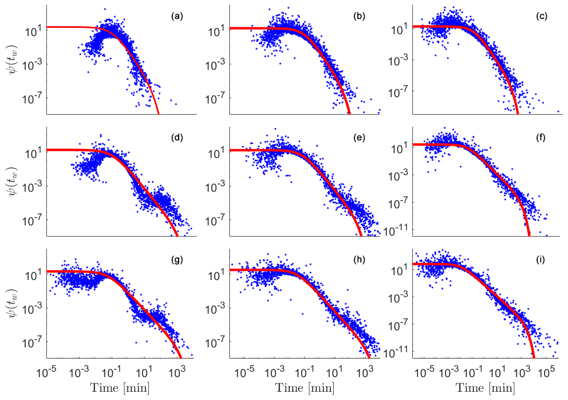
Figure 2 Sample and modeled probability density function ψ(t_w) of particle waiting times for a tracer test performed on the conductivity field prior to reaction for those associated with reactive simulation times of 10 and 20 min. Results correspond to ${\mathit{\sigma }}_{\mathrm{0}}^{\mathrm{2}}$ = $\mathrm{1},\mathrm{3},\mathrm{5}$ (left, middle, and right columns, respectively) and t =0 (a–c), 10 (d–f), and 20 min (g–i). Values of TPL parameters estimated by calibrating model Eq. (6) on the sample distributions are listed in Table 1.

3 Results

We start our analyses by simulating transport of a non-reactive tracer across the generated heterogeneous conductivity domains. As log-conductivity variance increases, the range of conductivity values naturally increases, this being reflected in the distribution f(y_ij) (see, for example, Fig. 1a–c (blue circles)). The shape of weighted conductivity distributions, f(ny_ij), differs from the one of f(y_ij), consistent with the observation that particles are chiefly channeled towards preferential flow pathways. The latter distributions tend to be shifted towards high conductivity values and are characterized by an enhanced mean conductivity value as compared against their generated (unweighted) counterparts (see conductivity mean and weighted mean values in Table 1 and the results corresponding to the blue and red circles depicted in Fig. 1a–c). This shift is imprinted onto the probability density function (PDF) of the waiting times and onto its associated TPL parameters (see Fig. 2a–c), consistent with prior studies (Edery et al., 2014, 2016b; Edery, 2021). We then simulate reactive transport across the collection of generated fields, allowing for precipitation (and/or dissolution) of calcite and assessing the evolution of the conductivity field according to the Kozeny–Carman formulation introduced in Sect. 2. Conductivity, head, and velocity fields, as well as particle visitations, n_ij(t), associated with species h and co are sampled across time.

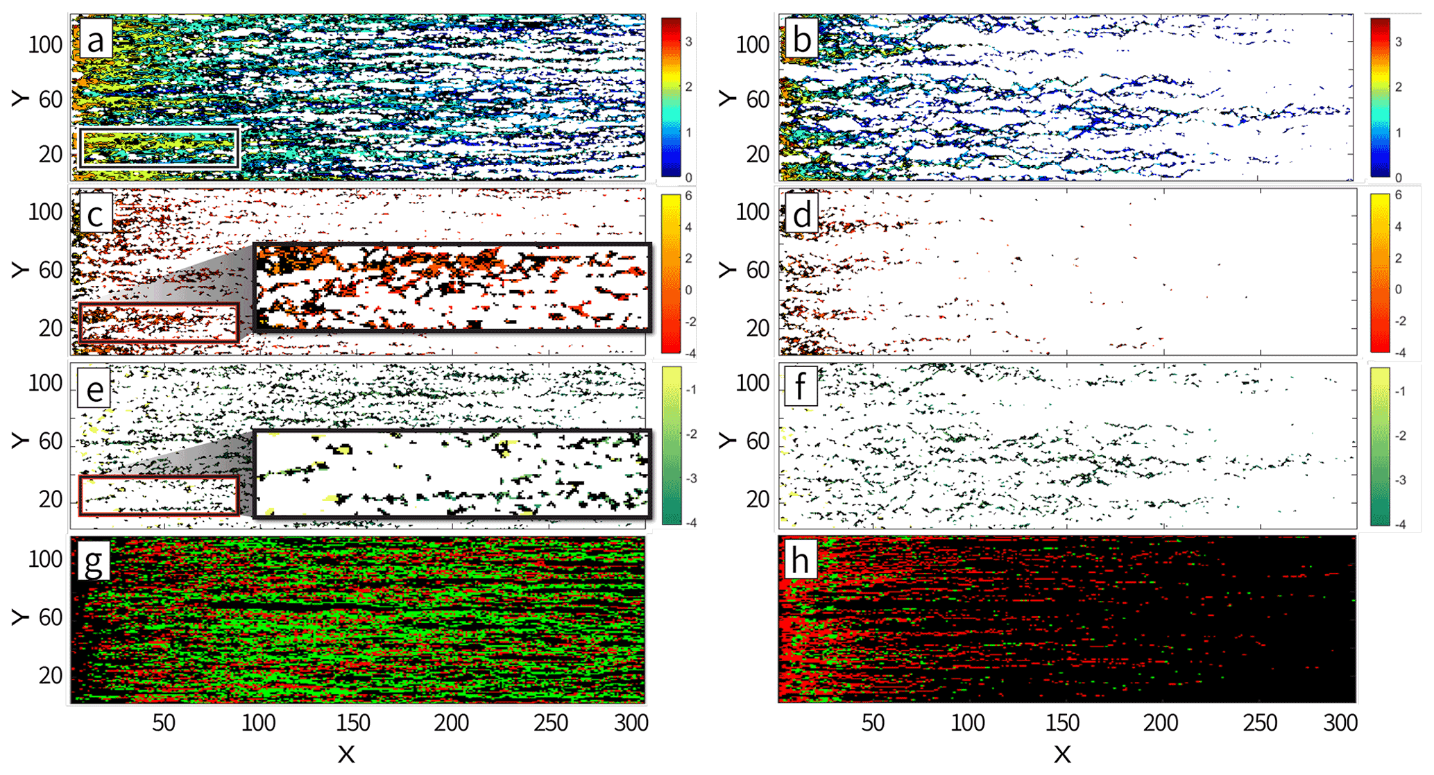
Figure 3 Heat map representing (a, b) log₁₀(n_Rij), i.e., the number of h particles visiting each cell for ${\mathit{\sigma }}_{\mathrm{0}}^{\mathrm{2}}$ = 1 and 5, respectively, and (c–f) relative change in hydraulic conductivity at time t = 20 min (corresponding to the first pore volume) with respect to the initially generated values for ${\mathit{\sigma }}_{\mathrm{0}}^{\mathrm{2}}$ = 1 (c, e) and ${\mathit{\sigma }}_{\mathrm{0}}^{\mathrm{2}}$ = 5 (d, f). Panels (c) and (d) display positive changes in conductivity with respect to the initial field, while panels (e) and (f) display negative changes in conductivity, with both positive and negative changes being represented on a log scale. Results correspond to a selected realization of the log-conductivity fields. The highlighted box illustrates the separation between regions where precipitation or dissolution take place. Panels (g) and (h) display cells associated with a net decrease (green) and increase (red) of conductivity for cells outside (g) or within the PF (h) for ${\mathit{\sigma }}_{\mathrm{0}}^{\mathrm{2}}$ = 1.

After 200 Δt has elapsed (corresponding to a total simulation time of 20 min, i.e., a full pore volume), a set of h particles connecting the inlet to the outlet of the system is clearly visible (see Fig. 3a and b), these particles being non-uniformly distributed in space. Figure 3a and b depict a heat map of the h particles distribution at time t = 20 min (i.e., corresponding to the first pore volume), clearly evidencing the emergence of regions of preferential flow (PF). We also note that the number of h particles density (corresponding to concentration) tends to decrease with increasing distance from the inlet, these being replaced by co particles, consistent with the observation that they are consumed during the course of the reactive process which induces dissolution of the host solid matrix. The h and co particles attain equilibrium within cells away from the inlet. As such, reaction can only take place if a particle leaves (or enters) a cell under the action of advection and/or diffusion, leading to a new equilibrium state. When examining the alteration of conductivities due to the dissolution/precipitation reaction, we note that dissolution (corresponding to an increase in permeability values) is primarily tied to the preferential flow pathways. Otherwise, precipitation is seen to take place in regions close (on average) to these pathways. The highest strength of precipitation is observed in the proximity of the preferential pathways and decreases with distance from these.

Figure 3c and e depict the regions where conductivity has increased (due to dissolution) or decreased (due to precipitation), respectively. The h particles invading the domain closely follow the PFs displaying a fingering pattern, leading to a corresponding dissolution pattern associated with locally increased conductivities. Since conductivity values along the PFs are typically higher (on average), dissolution is increasing these conductivities even further, giving rise to a self-sustained enhancing mechanism. The concentration of h particles reaches a local (i.e., within a given cell) equilibrium with the produced co particles. Hence, dissolution will take place where transport induces shifts in concentration that need to be compensated by the dissolution/precipitation process to maintain local equilibrium. Such scenarios can be attained (i) by co particles exiting the preferential flow pathways due to the action of diffusion (i.e., they leave locations where concentration of h particles is large upon diffusing towards higher pH regions where they precipitate) or (ii) by h particles traveling through the fast preferential paths and advancing through these. Figure 3g and h display regions with dominating dissolution or precipitation for cells outside and within the PFs, respectively. Here cells associated with PFs are identified upon relying on particle visitations following (Edery et al., 2014). Dissolution dominates within the PFs (as indicated by the red cells in Fig. 3h), because h particles are injected through a flux-weighted boundary condition. On the other hand, the produced co particles do not precipitate at locations corresponding to the high h concentration residing in the PFs. These may precipitate away from these regions, where they experience low concentrations of h particles. Thus, we observe a reduction of conductivity taking place in regions adjacent to the PFs (Fig. 3b and g). In summary, our computational results document an increase in conductivity along the preferential pathways jointly with a conductivity reduction within regions close to these and along directions approximately normal to them.

Changes in conductivity values ensuing precipitation/dissolution are clearly visible by the broadening of the unweighted log-conductivity distribution f(y_ij) (see Fig. 1d–f and g–i (blue circles), evaluated at times t = 10 and t = 20 min, respectively). The reaction dynamics lead to a conductivity field characterized by a slightly increased average value, given that our computational analyses entail the injection of an acid fluid into the system (see Table 1 for details). Detailed inspection of Fig. 1d and f reveals that precipitation takes place across a slightly larger area than dissolution; that is, values of the frequency distribution f(y_ij) associated with low conductivities tend to increase at a larger rate rather than those corresponding to high conductivities (the left tail of the distributions becomes heavier than the right tail with the progress of reaction). The weighted (f(ny_ij)) and unweighted (f(y_ij)) distributions (red and blue circles in Fig. 1d–f and g–i at times t = 10 and t = 20 min, respectively) are visibly broadening, being associated with an average conductivity which is higher than one of the originally generated conductivity domains (see Table 1). As stated above, dissolution is focused along the preferential pathways, which comprise an area of limited extent with respect to the whole field.

The above-documented mechanism and its signature on the weighted and unweighted conductivity frequency distributions are sensitive to the initial log-conductivity variance, ${\mathit{\sigma }}_{\mathrm{0}}^{\mathrm{2}}$. When considering both distributions f(y_ij) and f(ny_ij), associated with the case ${\mathit{\sigma }}_{\mathrm{0}}^{\mathrm{2}}=\mathrm{1}$, the distributions variance values are seen to increase in time, as compared to the values attained at the beginning of the simulation (i.e., prior to reaction; see Fig. 1a–d and g, as well as Table 1). Otherwise, as the initial heterogeneity increases (see, for example, ${\mathit{\sigma }}_{\mathrm{0}}^{\mathrm{2}}=\mathrm{3},\mathrm{5}$), mean and variance associated with the weighted and unweighted conductivity distributions display only minor changes (approximately 10 %) across the temporal window considered. The conductivity fields characterized by the lowest ${\mathit{\sigma }}_{\mathrm{0}}^{\mathrm{2}}$ value are associated with preferential pathways that are not starkly recognizable when analyzed under non-reactive transport conditions. These channels become more clearly distinguishable as reactions induce an increase in the conductivities along the PFs. At the same time, precipitation causes a decrease in the conductivity outside the PF. This leads to an increased importance of the left tail of f(y_ij), corresponding to an increase in low conductivity values (see Fig. 1, left, middle, and bottom rows).

With reference to the highest conductivity variance analyzed, the reaction patterns for the precipitation and dissolution lead to a smaller relative change between conductivity frequency distributions evaluated prior and after the reaction. Relative changes between the unweighted and weighted conductivity frequency distributions (including the ensuing mean and variance listed in Table 1) evaluated before and after the reaction are less pronounced as the variance in the generated conductivity field increases (see Fig. 1 (middle and right columns) and Table 1). This is related to the observation that, as log-conductivity variance increases, preferential pathways in the originally generated field become markedly more distinct. Thus, relative differences between unweighted and weighted conductivity histograms are seen to diminish in time, because the flow field is already organized according to well-identified pathways and tends to preserve its initial pattern (Fig. 1d–f and g–i at times t = 10 and t = 20 min, respectively). Note that low-order statistics (i.e., mean and variance) of velocity and conductivity display only a minute evolution with the progress of reaction, in spite of the relevant changes exhibited by the tails of the frequency distributions (see Fig. 1) for all considered values of ${\mathit{\sigma }}_{\mathrm{0}}^{\mathrm{2}}$, with the latter feature being relevant when addressing non-Fickian transport, as further discussed below.

As stated in Sect. 2.2, the conductivity fields altered through precipitation/dissolution and extracted at regular time intervals of 10 Δt are subject to non-reactive transport analyses, and the ensuing evolution of the parameters of the TPL model (Eq. 6) is analyzed. Key results of these analyses are listed in Table 1 with reference to the original (unaltered) conductivity fields and at the final simulation time (i.e., at time t = 200 Δt). Analysis of the results associated with transport across the log-conductivity field characterized by the smallest original variance (i.e., ${\mathit{\sigma }}_{\mathrm{0}}^{\mathrm{2}}$ = 1) and listed in Table 1 indicates that the changes in the sample log-conductivity PDF induced by the progress of the reaction are reflected by the parameters of the TPL model (Eq. 6). These transition from estimated values corresponding to an effective Fickian transport regime (corresponding to β=2; see also Fig. 2a) to values denoting a highly non-Fickian effective transport setting, manifested by the widening of the support of the waiting time PDF ψ(t_w) (see also Fig. 2d and g for results obtained at t = 10 and 20 min, respectively). Effective transport in the domain with the highest variance (i.e., ${\mathit{\sigma }}_{\mathrm{0}}^{\mathrm{2}}$ = 5; see Table 1) is characterized by estimated TPL parameters corresponding to a non-Fickian signature also prior to the occurrence of precipitation/dissolution (Fig. 2c). Such a signature is then further enhanced after reaction has altered the conductivity field yet displaying a less marked evolution of the shape of the ψ(t_w) as compared to the case ${\mathit{\sigma }}_{\mathrm{0}}^{\mathrm{2}}$ = 1 (see also Fig. 2f and i for t = 10 and 20 min, respectively).

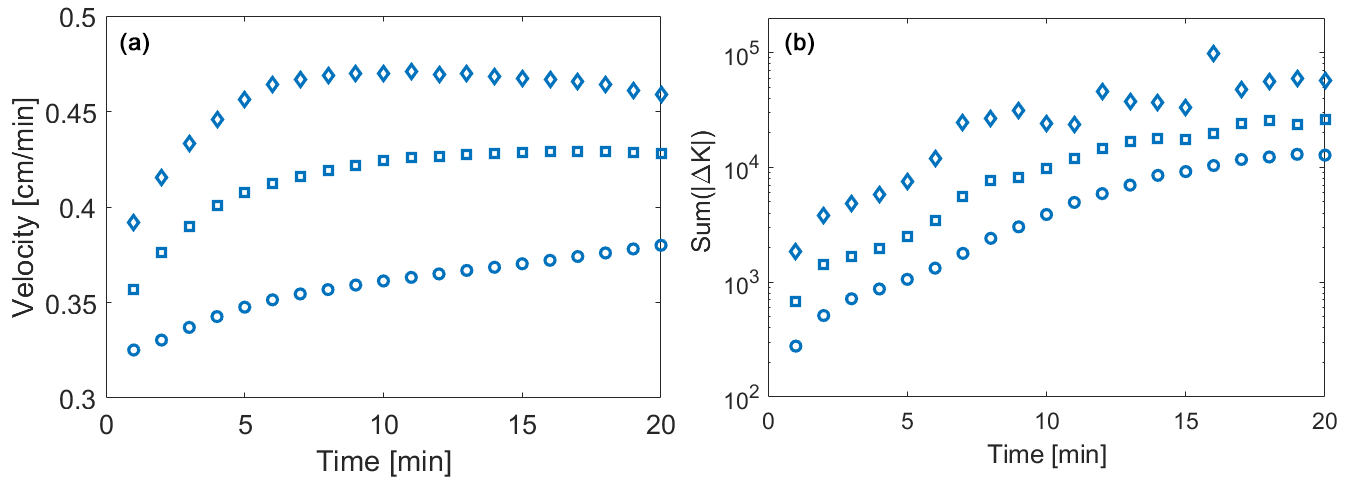
Figure 4 Temporal evolution of (a) the weighted mean velocity $\stackrel{\mathrm{‾}}{n_{\mathrm{R}}v}$ (open symbols) and (b) the sum of all conductivity changes over 1 min. Results correspond to ${\mathit{\sigma }}_{\mathrm{0}}^{\mathrm{2}}$ = 1 (circles), 3 (squares), and 5 (diamonds).

The observed temporal changes in conductivity and the ensuing local dynamics of transport pattern yield global variations in the reaction rate. Consistent with prior studies and the imposed boundary conditions, the mean velocity associated with the originally generated conductivity domains increases with ${\mathit{\sigma }}_{\mathrm{0}}^{\mathrm{2}}$. As the reaction progresses and the conductivity fields change, the increased area subject to dissolution leads to a slight increase in the mean velocity for all of the ${\mathit{\sigma }}_{\mathrm{0}}^{\mathrm{2}}$ analyzed. To analyze the influence of the preferential flow on the velocity that is affecting particle transport, we consider the average value $\stackrel{\mathrm{‾}}{n_{\mathrm{R}}v}$, evaluated upon considering weighting by the number of reactive particles, n_R, visiting each cell (where the term reactive particles denotes both h and co particles employed in the context of the reactive transport simulations). The weighted average velocity displays an initial increase over time due to the increase in conductivity within the preferential pathways. When considering the relative change across the whole simulation time, values of the temporal increase in $\stackrel{\mathrm{‾}}{n_{\mathrm{R}}v}$ are similar across the three heterogeneity levels examined, i.e., they are seemingly independent of ${\mathit{\sigma }}_{\mathrm{0}}^{\mathrm{2}}$. However, results in Fig. 4a also reveal that the average velocity $\stackrel{\mathrm{‾}}{n_{\mathrm{R}}v}$ displays distinct temporal histories depending on ${\mathit{\sigma }}_{\mathrm{0}}^{\mathrm{2}}$. In particular, the value of $\stackrel{\mathrm{‾}}{n_{\mathrm{R}}v}$ tends to attain an asymptotic value at time t ≈ 7 min for ${\mathit{\sigma }}_{\mathrm{0}}^{\mathrm{2}}=\mathrm{5}$, while showing a sustained increasing trend for ${\mathit{\sigma }}_{\mathrm{0}}^{\mathrm{2}}=\mathrm{1}$. This result suggests that the feedback between reaction and flow patterns reaches an asymptotic condition faster in systems characterized by higher heterogeneity.

The temporal evolution of the velocity fields due to the precipitation/dissolution reaction and the resulting conductivity changes lead to a time-dependent reaction pattern and reaction rates. The Damköhler number is infinite on a local scale in our computational analyses, because the reaction is instantaneous. When considering the entire system, transport processes induce a net overall reaction rate that can be quantified as the sum of the total conductivity changes across time (Sum(|Δk_ij|) [cm s⁻¹]). The latter incorporates both positive and negative changes in hydraulic conductivity and therefore quantifies the overall intensity of precipitation and dissolution processes in the domain. The quantity Sum(|Δk_ij|) is evaluated across all realizations for each of the ${\mathit{\sigma }}_{\mathrm{0}}^{\mathrm{2}}$ values considered and is depicted in Fig. 4b as a function of time. These results indicate that the overall reaction rate increases in time with a similar rate for all considered values of ${\mathit{\sigma }}_{\mathrm{0}}^{\mathrm{2}}$ (Fig. 4b) at early times. The observed increase is consistent with the initial advancement of the reaction front across the domain. We observe that the reactive process magnitude is proportional to ${\mathit{\sigma }}_{\mathrm{0}}^{\mathrm{2}}$. For low initial levels of heterogeneity, conductivity values along the preferential pathways are closer to the average field conductivity than what can be observed for the highly heterogeneous domains. As such, the portion of the domain where precipitation or dissolution can take place increases at a rate proportional to ${\mathit{\sigma }}_{\mathrm{0}}^{\mathrm{2}}$. As the reaction front reaches the domain outlet, the dissolving front found in the PF leaves the domain. Hence, the global variation in conductivity (which is proportional to the magnitude of reactive processes) tends towards an asymptotic value, corresponding to the diffusion-controlled solute exchange along a direction transverse to the preferential pathways (see Fig. 3). In agreement with results shown in Fig. 4a, this transition towards an asymptotic regime takes place earlier for larger values of ${\mathit{\sigma }}_{\mathrm{0}}^{\mathrm{2}}$, while a smaller initial heterogeneity implies a longer transient period.

4 Conclusions

Our computational study tackles the quantitative characterization of the feedbacks between precipitation and dissolution reaction dynamics taking place in randomly heterogeneous conductivity fields associated with various degrees of spatial heterogeneity. Our work leads to the following key conclusions.

Joint occurrence of precipitation and dissolution is tightly coupled with the existence of preferential flow pathways. Conductivity increase due to the dissolution reaction along such paths leads to enhanced particle migration along these. The dominance of preexisting preferential flow regions on the (reactive) transport pattern across the field is therefore further reinforced and self-sustained across time. At the same time, diffusion promotes displacement of particles, leading to precipitation (and hence a progressive reduction over time of local conductivities) at locations in the proximity of these.

Reactive processes yield an increase over time of the range of conductivity values across the domain, eventually leading to a widening of the support of solute waiting times and conductivity distributions. The clear separation between regions where dissolution or precipitation takes place is reflected in sample distributions of conductivity which tend to become visibly left skewed with time, a feature which is associated with precipitation taking place in low-conductivity cells located in the proximity of existing preferential flow pathways.

We weight the conductivity and velocity distributions with the solute mass, to characterize the probability density function of particle travel/waiting times, which form the TPL model parameters, thus enabling us to capture effective (upscaled) non-Fickian transport behaviors. With the progress of precipitation/dissolution reactions, transport shifts towards an increasingly acute non-Fickian effective behavior (see Fig. 2 and ensuing parameter values listed in Table 1). The latter is then seen as a direct outcome of the documented feedbacks between transport and reactions taking place in heterogeneous porous media. The evolution of TPL model parameters towards a pronounced non-Fickian behavior is associated with only minor changes in the mean and variance of log-conductivity values. This result is consistent with the conceptual picture that the tails of flux and hydraulic conductivity distributions carry critical information to characterize transport while displaying only a minor effect on low-order statistics associated with these quantities. Our results suggest that this feature must be acknowledged to properly characterize transport in the presence of precipitation/dissolution. In this context, we recall that our study is not aimed at exploring the skill of any specific transport model to interpret non-reactive transport across the conductivity fields prior and/or after reaction takes place, with this particular analysis being deferred to a future study.

We observe the emergence of an asymptotic regime in highly heterogeneous systems, where the (averaged) solute velocity attains a constant value even in the presence of reaction. This suggests the occurrence of an equilibrium state between reactive processes and transport under the flow conditions analyzed. This regime is attained because the effects of locally occurring precipitation and dissolution balance each other at the overall scale of the system, so the ensuing (ensemble-averaged) solute velocity remains unaffected. The time required to attain such an asymptotic state increases with decreasing initial heterogeneity of the conductivity field, thus suggesting that pre-asymptotic behaviors may be more relevant in initially (i.e., prior to reaction taking place) homogeneous systems.

Our results are based on numerical simulations and may be used to inform upscaling approaches to capture the pre-asymptotic and asymptotic dynamics of reactive transport in heterogeneous systems through simplified models. Future computational studies might also include an assessment of the importance of initial/boundary conditions and/or of solute injection mode on the emergence of non-Fickian transport features, with special emphasis on locations close to the inlet boundary which might then have an impact on the overall solute residence times and related statistics.