Spatiotemporal and cross-scale interactions in hydroclimate variability: a case-study in France

Understanding how water resources vary in response to climate at different temporal and spatial scales is crucial to inform long-term management. Climate change impacts and induced trends may indeed be substantially modulated by low-frequency (multi-year) variations, whose strength varies in time and space, with large consequences for risk forecasting systems. In this study, we present a spatial classification of precipitation, temperature, and discharge variability in France, based on a fuzzy clustering and wavelet spectra of 152 near-natural watersheds between 1958 and 2008. We also explore phase–phase and phase–amplitude causal interactions between timescales of each homogeneous region. A total of three significant timescales of variability are found in precipitation, temperature, and discharge, i.e., 1, 2–4, and 5–8 years. The magnitude of these timescales of variability is, however, not constant over the different regions. For instance, southern regions are markedly different from other regions, with much lower (5–8 years) variability and much larger (2–4 years) variability. Several temporal changes in precipitation, temperature, and discharge variability are identified during the 1980s and 1990s. Notably, in the southern regions of France, we note a decrease in annual temperature variability in the mid 1990s. Investigating cross-scale interactions, our study reveals causal and bi-directional relationships between higher- and lower-frequency variability, which may feature interactions within the coupled land–ocean–atmosphere systems. Interestingly, however, even though time frequency patterns (occurrence and timing of timescales of variability) were similar between regions, cross-scale interactions are far much complex, differ between regions, and are not systematically transferred from climate (precipitation and temperature) to hydrological variability (discharge). Phase–amplitude interactions are indeed absent in discharge variability, although significant phase–amplitude interactions are found in precipitation and temperature. This suggests that watershed characteristics cancel the negative feedback systems found in precipitation and temperature. This study allows for a multi-timescale representation of hydroclimate variability in France and provides unique insight into the complex nonlinear dynamics of this variability and its predictability.

1 Introduction

Hydroclimate variability represents the spatiotemporal evolution of hydrological (e.g., discharge and groundwater level) and climate variables (e.g., precipitation and temperature) which are directly impacting hydrological variability. Studying how hydrological variables react to climate variability and change is a major challenge for society, in particular for water resource management and flood and drought mitigation planning (IPCC, 2007, 2014, 2021). However, hydrological variability is expressed at multiple timescales (Labat, 2006; Schaefli et al., 2007; Massei et al., 2007, 2017), for which the driving mechanisms remain poorly characterized and understood. As suggested in Blöschl et al. (2019), understanding the spatiotemporal scaling, i.e., how the general dynamics driving hydrological variability change at spatial and temporal scales, represents a major challenge toward improved prediction systems (Gentine et al., 2012). Understanding spatiotemporal scaling required to identify regions, i.e., the maximum spatial scale in which the dynamics remain unchanged despite its nonlinearity, is critical (Hubert, 2001). Hydrological variability is, by definition, nonlinear (Labat, 2000; Lavers et al., 2010; McGregor, 2017) as it results from complex interactions between atmospheric dynamics and catchment properties that may vary at different timescales (e.g., soil characteristics, water table, karstic systems, and vegetation covers; Gudmundsson et al., 2011; Sidibe et al., 2019). Such interactions between processes at different timescales, i.e., cross-scale interactions (Palus, 2014; Jajcay et al., 2018), have never been studied to further understand hydrological variability. It has also been shown that hydroclimate variability is inherently nonstationary, with the time dependence of the mean and variance due to changes in the controlling factors (e.g., Coulibaly and Burn, 2004; Labat, 2006; Dieppois et al., 2013, 2016; Massei et al., 2017). This results in difficulties in characterizing and predicting the hydrological variability at different spatiotemporal scales (Gentine et al., 2012; Blöschl et al., 2019).

While different timescales have been identified in hydrological variability (Coulibaly and Burn, 2004; Labat, 2006; Dieppois et al., 2013, 2016; Massei et al., 2017), very little has been done to (i) explore how spatially coherent those timescales are and (ii) identify regions in which the statistical characteristics of all ranges of variability remain unchanged. Studying 231 stream gauges throughout the world, Labat (2006) highlighted different timescales of discharge variability over the different continents. At the regional scale, Smith et al. (1998) established a clustering of 91 USA stream gauges based on their global wavelet spectra, i.e., dominant timescales, and found five homogeneous regions. Similarly, Anctil and Coulibaly (2004) and Coulibaly and Burn (2004) established a clustering of southern Quebec and Canadian streamflow, based on the timing of both the 2–3- and 3–6-year timescales. In Europe, Gudmundsson et al. (2011) identified different regions according to the magnitude of decadal discharge variability. In France, such a clustering, based on time frequency patterns of discharge variability, and its relation to climate variability (e.g., precipitation and temperature), has not yet been explored. In addition, all studies mentioned above either isolated particular timescales of variability or averaged the variability across timescales (e.g., global wavelet spectra), which is equivalent to a linearization of the system (Hubert et al., 1989). These studies thus ignore potential feedback mechanisms, e.g., between soil moisture, precipitation, and temperature (Materia et al., 2021; Ardilouze et al., 2020; Bellucci et al., 2015). In the presence of feedback mechanisms, interactions occur over different timescales, which are also called cross-scale interactions (Christophe Bouton, 2017). However, while studying cross-scale interactions has gained increasing interest in other fields, such as neurosciences (e.g., Onslow et al., 2014; Wang et al., 2014), cross-scale interactions are poorly understood in climate and hydrological sciences. New strategies have recently been developed to facilitate such studies (Jajcay et al., 2018). Cross-scale interactions are, however, very relevant to hydroclimate studies, in particular when searching for climate drivers (or predictors) of hydrological signals, as they will reveal climate timescales that are causality linked to each timescale of hydrological variability.

In this study, we investigate the spatial homogeneity of hydroclimate variability in France across timescales. We aim at identifying homogeneous regions according to specific time frequency patterns. From the determination of homogeneous regions of hydroclimate variability, we will explore cross-scale interactions that may result from feedback processes between catchment properties and hydroclimate variability.

This study, therefore, has major implications for the comprehension of hydroclimate dynamics and their interactions with large-scale climate drivers and catchment properties. In addition, as recently suggested in Scaife and Smith (2018), improved characterization of the different timescales of variability and their interactions could help optimize ensemble-based hydrological forecasting systems through identifying climate ensemble members that better match the observed realization.

The work is divided into the following sections. Data and methods are introduced in Sect. 2. In Sect. 3, we establish homogeneous regions for precipitation, temperature, and discharge variability based on their time frequency patterns and then explore cross-scale interactions for each region of homogeneous variability in precipitation, temperature, and discharge. Finally, discussions of the main results and conclusions are provided in Sect. 4.

.

Figure 1 Location of stream gauges (gray dots), corresponding watersheds (pale red; Brigode et al., 2020), hydrographic network (blue lines; Pella et al., 2012), and orography in Safran data set (grayscale; Vidal et al., 2010)

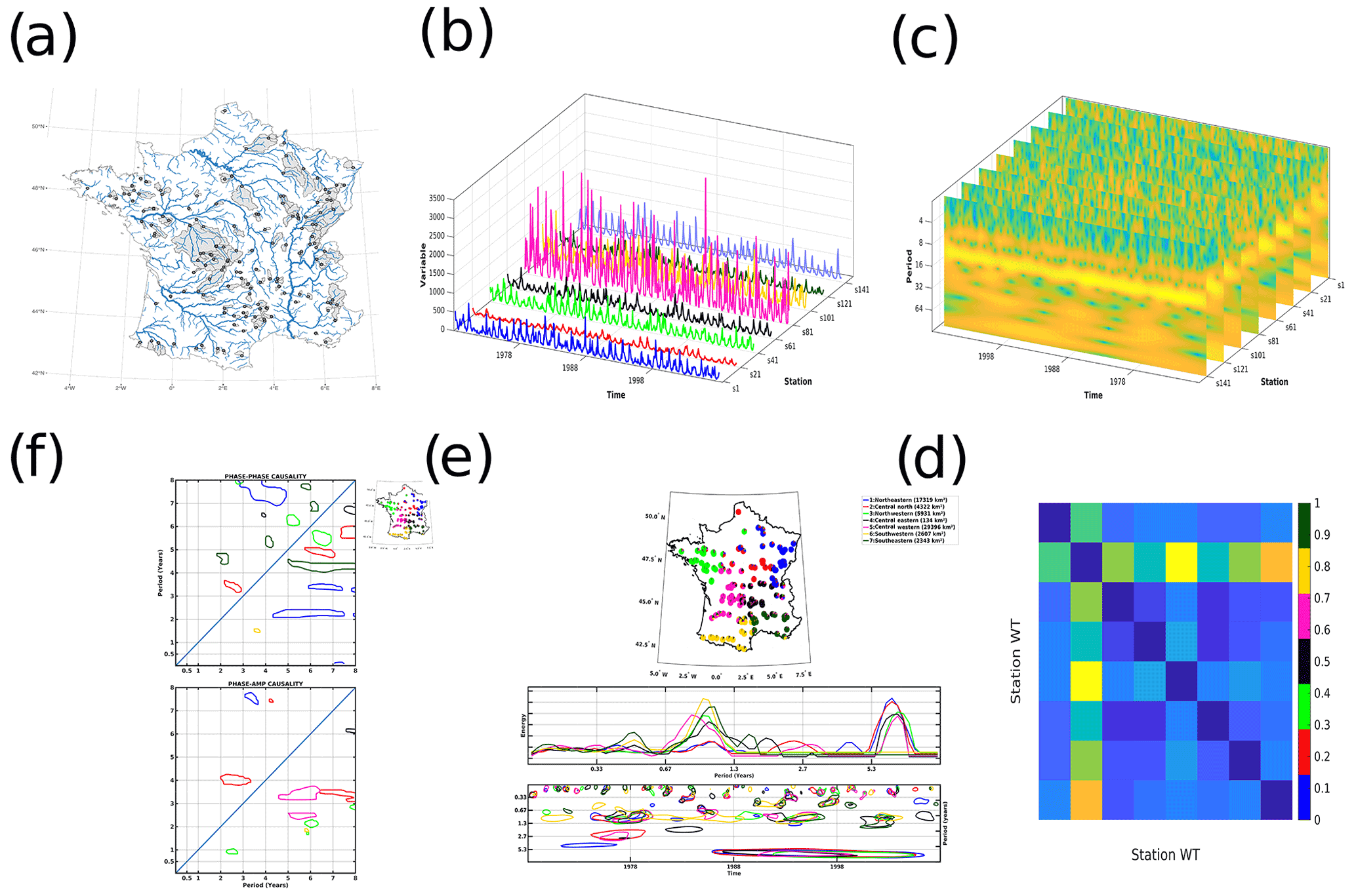
Figure 2 The workflow of this study is repeated for precipitation, temperature, and discharge data sets. (a) A total of 152 near-natural watersheds are selected. (b) Each watershed is represented by a monthly time series from 1968 to 2008, discharge is measured at a gauging station, and precipitation and temperature are averaged over the watershed. (c) The continuous wavelet transform of each time series is computed, representing the timescale-dependent, nonstationary variability in each watershed. (d) The similarity between all 152 continuous wavelet transforms is computed and represented as a distance matrix. (e) Similar watersheds are grouped together into regions of homogeneous variability using a fuzzy clustering algorithm (top). For each region, the relative importance of each timescale-dependent variability is represented with a global wavelet spectrum, and global wavelet spectra are superimposed for all regions (middle). The continuous wavelet spectra of the regions are superimposed (bottom). For clarity, only timescale and time locations with the most significant variability are shown (colored circles). (f) For each region, cross-timescale interactions are computed. The phase–phase interactions (top) identify any timescale's phase that conditions another timescale's phase. The phase–amplitude interactions (bottom) characterize any timescale's phase that conditions the amplitude of another timescale.

2 Data and methodology

2.1 Hydrological and climate data

The data consist of precipitation, temperature, and discharge time series located over 152 watersheds (Figs. 1, 2a and b). Discharge time series were extracted from French reference hydrometric network compiled by Giuntoli et al. (2013). This network of stations identifies near-natural watersheds (i.e., with negligible anthropogenic modifications) with long-term, high-quality hydrometric data. According to Giuntoli et al. (2013), this subset of stations does not show abrupt changes and trends that could have resulted from anthropogenic influence. The period of 1968–2008 was chosen by Giuntoli et al. (2013) as being the best trade-off in terms of data availability over the different regions. Here, this database was further subset to 152 watersheds in order to select complete monthly time series (i.e., without missing values) only (Fig. 1). Precipitation and temperature data have been estimated from the 8 km grid Safran surface reanalysis data set (Vidal et al., 2010) and have been subset to a common period (1968–2008). For this study, precipitation and temperature have been averaged over each watershed area (Caillouet et al., 2017). Each station is thus representative of one watershed.

2.2 Methods

The methodology described below (and summarized in the workflow in Fig. 2) is applied to precipitation, temperature, and discharge data sets.

2.2.1 Continuous wavelet transforms

For each of the 152 watersheds, continuous wavelet analysis is used to identify at which timescales and time locations the amplitude of variability (i.e., local variance) is the strongest (Fig. 2c; Torrence and Compo, 1998). Here we employ the words timescale and frequency interchangeably, though frequency implies a periodic variability, which is not a necessary condition in continuous wavelet analysis. For any finite energy signal x, it is possible to obtain a time frequency representation by projecting the time series onto a function called the mother wavelet, which quantifies the amplitude of the time series variability at a given timescale and time location. This mother wavelet can be translated in time to quantify the variability at precise time locations but can also be scaled so that variability at different timescales can be quantified as well (Torrence and Compo, 1998; Grinsted et al., 2004). A mother wavelet at a timescale a and time location b is called a daughter wavelet. Daughter wavelets are calculated as follows:

$$\begin{array}{}\text{(1)}& {\mathit{\psi }}_{a,b}={\displaystyle \frac{\mathrm{1}}{\sqrt{a}}}\mathit{\psi }\left({\displaystyle \frac{t-b}{a}}\right).\end{array}$$

The left-hand side (LHS) term is the daughter wavelet of scale a and time translation b at time t. For the sake of simplicity, we will refer to b as the time location. The first right-hand side (RHS) term is the scaling of the mother wavelet ψ, and the last one is the time translation. The projection of the signal onto each scale a takes the following form:

$$\begin{array}{}\text{(2)}& {\text{WT}}_{\mathit{\psi }}\left[x\right](a,b)=\langle x,{\mathit{\psi }}_{a,b}\rangle =\underset{R}{\int }x\left(t\right){\mathit{\psi }}_{a,b}\left(t\right)\mathrm{d}t.\end{array}$$

The LHS term contains the wavelet coefficients, WT, i.e., how large the amplitude of variability at the timescale a and time location b is. If the mother wavelet (and, hence, the daughter wavelets as well) is complex, wavelet coefficients are complex as well, and both the amplitude and instantaneous phase of the time series can be computed around time location b and timescale a. Wavelet coefficients represent the inner product of the signal, the daughter wavelet of scale a, and the time location b (center). The norm of their square is called the wavelet power and represents the amplitude of the oscillation of signal x at scale a and centered on time location b. As it is impossible to capture the best resolution in both timescale and time location simultaneously, here we used a Morlet mother wavelet (of the order of 6), which offers a good trade-off between the detection of scales and localization of the oscillations in time (Torrence and Compo, 1998). Visualization of a continuous wavelet transform is called a scalogram. Figure 2c shows a collection of scalograms, with the time location on the horizontal axis and timescale on the vertical axis. Yellow colors show the timescales and time locations when the amplitude of the time series' variability is maximum. A major advantage of continuous wavelet transform, compared to other signal analysis methods such as the Fourier transform, is that wavelet analysis takes nonstationarity into account. Nonstationarity is the time location dependence of both the mean and variance of a time series.

Because the daughter wavelet translates and scales up, overlaps in time and frequency can occur, and wavelet coefficients can be overestimated, requiring statistical significance tests (Torrence and Compo, 1998). This redundancy may give rise to peaks in the wavelet coefficients (meaning that high variability is detected) even in the case of a random noise (Ge, 2007). Torrence and Compo (1998) used Monte Carlo simulations to assess the statistical significance of the continuous wavelet transform of their time series. Just as with any other statistical analysis, the performance of statistical tests is an open debate. It has been shown that, while the significance test of Torrence and Compo (1998) may not unravel all significant wavelet coefficients, their false detection rate is low for as long as the mother wavelet chosen is adapted to the time series (Ge, 2007). By using a Morlet wavelet of the order of 6, we ensure that such statistical significance tests keep the false detection rate low (Ge, 2007). Because the significance test's aim is to ensure that large peaks are exceeding the range of variability that would occur in a random noise, statistically significant wavelet coefficients are always those with large wavelet coefficients values for any given timescale.

For the reminder of this study, the terms intraseasonal, annual, and interannual refer to variations at <1-, 1-, 2–4-, and 5–8-year timescales, respectively.

2.2.2 Image Euclidean distance clustering

After each watershed wavelet spectrum is computed, we estimate the similarity between them, i.e., how similar the variability is, for given scales and time locations, among all wavelet spectra (Fig. 2d). Similarities between wavelet spectra are estimated from the entire wavelet spectrum, and not only on statistically significant signals, to guarantee more consistent comparison between spectra. Distances between two-dimensional data, such as wavelet spectra, are estimated using Euclidean distance between pairwise points (pED; i.e., computing $f_{\mathrm{2}}(x_i,y_i)-f_{\mathrm{1}}(x_i,y_i)$). However, such a procedure has no neighborhood notion, making it impossible to account for globally similar shapes (Wang et al., 2005). To avoid this issue, we used the image Euclidean distance calculation method (hereinafter IEDC) developed by Wang et al. (2005). The IEDC method modifies the pED equation in the following two ways (Wang et al., 2005): (i) the distance between pixel values is computed not only pairwise but for all indices, and (ii) a Gaussian filter, a function of the spatial distance between pixels, is applied. The Gaussian filter then applies less weight to the computed distance between very close and far apart pixels, while emphasizing on medium-spaced ones (Wang et al., 2005).

2.2.3 Fuzzy clustering

Fuzzy clustering has then been used to cluster the different watersheds based on their similarities (Fig. 2e). Fuzzy clustering is a soft clustering method (Dunn, 1973). While soft clustering spreads membership over all clusters with varying probability, hard clustering attributes each station one, and only one, cluster membership. Soft clustering is therefore better suited to situations when the spatial variability, originating from different stations' hydroclimate characteristics, is smooth. For instance, precipitation and temperature patterns are unlikely to change suddenly from one station to a neighboring one and in turn, be markedly different from the next neighbor (Moron et al., 2007; Hannaford et al., 2009; Rahiz and New, 2012). As such, several stations tend to show transitional or hybrid patterns and can potentially be members of different clusters, limiting the robustness of hard clustering procedure (Liu and Graham, 2018).

Fuzzy clustering performance is determined by the ability of the algorithms to recognize hybrid stations (i.e., stations incorporating multiple features from different patterns observed in other coherent regions), while allowing for a clear determination of the membership of stations with unique features (Kaufman and Rousseeuw, 1990). Here, we used the FANNY algorithm (Kaufman and Rousseeuw, 1990), which has been shown to be flexible and to offer the possibility to adapt the clustering to the data with optimal performance (Liu and Graham, 2018). In addition, rather than setting the number of clusters arbitrarily, we used an estimation of the optimum number of clusters by first computing a hard clustering method, namely consensus clustering (Monti et al., 2003). Thus, the number of clusters providing the best stability (i.e., the minimal changes in membership when adding new individuals) is considered optimal, as recommended in Şenbabaoǧlu et al. (2014). The different clusters' memberships are then mapped to discuss the spatial coherence of each hydroclimate variable.

2.2.4 Cross-scale interactions

For each variable and each cluster, cross-scale interactions are explored (Fig. 2f). Cross-scale interactions refer to phase–phase and phase–amplitude couplings between timescales of a given time series (Paluš, 2014; Scheffer-Teixeira and Tort, 2016). Here, coupling means that the state (either phase or amplitude) of a signal y is dependent on the state of a signal x and describes causal relationship (Granger, 1969; Pikovsky et al., 2001), which refers to the information transfer from a timescale of one signal to another.

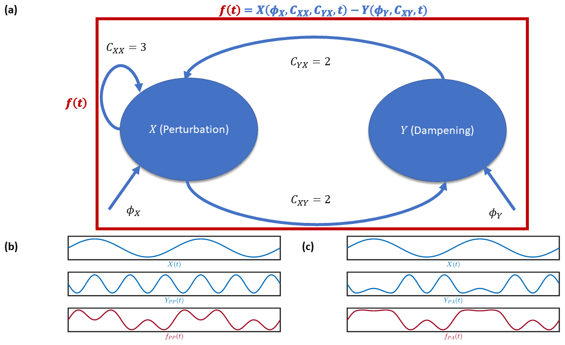
Figure 3 A system with directional cross-scale interactions. (a) A variable f(t) made of two components, X and Y, connected through C_XY and C_YX in a perturbation–dampening scheme, so that $f\left(t\right)=X\left(t\right)-Y\left(t\right)$. Both X and Y receive inputs ϕ_X and ϕ_Y, respectively. C_XX allows X to grow first. Depending on both inputs and connections, some phase–phase or phase–amplitude interactions between X and Y can occur. (b) An example of a phase–phase interaction, with every fourth ridge of Y_PP coinciding with a ridge of X, with $f_{\mathrm{PP}}\left(t\right)=X\left(t\right)-Y_{\mathrm{PP}}\left(t\right)$ (top, middle, and bottom panels, respectively). (c) An example of a phase–amplitude interaction. X and Y_PA only interact when X reaches a ridge, in which case the Y_PA amplitude, if lowered, yields f_PA(t) (top, middle, and bottom panels, respectively; adapted from Onslow et al., 2014).

Figure 3 describes the necessary setting and characteristics of cross-scale interactions. A variable (f) measures the dynamics of a system (e.g., precipitation or temperature variability). This system is modeled as a coupling of two components (X and Y). The components interact with each other in a perturbation–dampening (X and Y, respectively) scheme so that $f\left(t\right)=X(..,t)-Y(..,t)$ (Fig. 3a). The interactions between the components occur through the connections C_XY and C_YX, with a given strength (here $C_{..}=\mathrm{2}$), and this perturbation–dampening interaction forms a negative feedback (i.e., an increase in X activity triggers Y activity and dampens X activity, which, in turn, lowers X activity, thus lowering Y activity, thus allowing X activity to increase again, and so on; Fig. 3a). The connection C_XX enables X to grow first before Y dampens it. This connection C_XX forms a positive feedback, i.e., increases in X activity will be more severe as X activity is high. Both X and Y receive inputs ϕ_X and ϕ_Y from driving processes (e.g., moisture advection and convective processes; Fig. 3a). Depending on both the mean and timescales of ϕ_X and ϕ_Y, the strength of C_XX, C_XY and C_YX, and X and Y may show coupled behaviors. For instance, in Fig. 3b, every fourth ridge of Y_PP(t) is synchronized with a ridge of X(t) (Fig. 3b; top and middle panels), thus forming a phase–phase interaction. The direction of the interactions depends on the inputs (ϕ_X, ϕ_Y) and the connections (C_XX, C_XY, and C_YX). f_PP(t) is the difference between X(t) and Y_PP (Fig. 3b; bottom panel). Because the interaction between X and Y depends on both inputs and connections, interactions may lead to a cross-scale relationship only for certain values of X or Y (Fig. 3c). Thus, depending on the phase of either X or Y, the amplitude of the driven component may increase/decrease when the cross-scale interaction takes place and return to normal when it is out of phase compared to the driving component. This describes a phase–amplitude interaction. In Fig. 3b, Y_PA amplitude decreases when X is at its maximum (i.e., when its phase is a ridge; Fig. 3c; top and middle panels). Similar to the phase–phase interaction, f_PA(t) is the difference between X(t) and Y_PA(t) (Fig. 3c; bottom panel). Because phase and amplitude are very dependent on inputs ϕ_X and ϕ_Y, connections between spatially distant physical processes are likely to give rise to phase–amplitude interactions (Nandi et al., 2019). In summary, there are three elements needed for cross-scale interactions between multiple, coupled processes, to arise, namely that (i) an oscillating forcing ϕ_X must drive X and an additional forcing ϕ_Y on Y may also be present, (ii) X must have positive feedback on itself so that it grows faster than Y;, and(iii) Y must show a dampening effect on X (XY or YX negative feedback). The presence and characteristics of cross-scale interactions depend on the strength and frequencies of ϕ_X,ϕ_Y, intrinsic frequencies of X,Y, and coupling strengths C_XY, C_YX, C_XX, and C_YY (Fig. 3). Thus, the detection of cross-scale interactions in time series is an indication of the presence of all those characteristics in the hydroclimate system, e.g., precipitation–land processes, which helps in investigating potential processes at play.

The balance between X and Y determines if the feedback is either positive or negative (Peters et al., 2007).

Note that cross-scale interactions can occur from large-scale to small-scale processes and vice-versa. For instance, atmospheric circulation at seasonal timescales influences interannual and decadal timescales, which, in turn, influences seasonal variations (Hannachi et al., 2017).

Following Palus (2014) and Jajcay et al. (2018), we chose the conditional mutual information (CMI) surrogates method, combined with wavelet transforms. First, using a Morlet mother wavelet, the instantaneous phase and amplitude at time t and scale s of the signal are obtained. Next, the conditional mutual information, $I\left({\mathit{\varphi }}_x\right(t);{\mathit{\varphi }}_y(t+\mathit{\tau })-{\mathit{\varphi }}_y(t\left)\right|{\mathit{\varphi }}_y\left(t\right))$, for the phase, and $I\left({\mathit{\varphi }}_x\right(t);A_y(t+\mathit{\tau }\left)\right|A_y\left(t\right)),A_y(t-\mathit{\eta }\left)\right),A_y(t-\mathrm{2}\mathit{\eta }))$, for the amplitude, is computed. In the case of phase–phase relationships, the CMI measures how much the present phase of x contains information about the future phase of y, knowing the present value of y. Phase–phase interactions can be uni- or bi-directional. It is possible for a single timescale to drive another, which, in turn, drives back the original one, describing feedback interactions. For phase–amplitude relationships, CMI measures how much the present phase of x contains information of the future amplitude of y, knowing the present and past values of y. The statistical significance of the CMI measure is assessed using 5000 phase-randomized surrogates having the same Fourier spectrum and mean and standard deviation as the original time series, as seen in Ebisuzaki (1997). Palus (2014) has shown that this number of surrogates is ideal for statistical significance in the context of hydroclimate time series. The computational cost is, however, high, with approximately 1 week of computing for a time series of 50 years on a 32 core Xeon computer. The present computations were done on the Myria cluster, hosted by the Centre Régional Informatique et d'Applications Numérique de Normandie (http://www.criann.fr; last access: 7 January 2021).

3 Spatiotemporal clustering of hydrological variability

The wavelet transform corresponding to each watershed's monthly time series have been computed, and all 152 watersheds' wavelet transforms have been checked for similarities using IEDC fuzzy clustering to identify and characterize homogeneous regions of hydroclimate variability over France. Once the homogeneous regions had been identified, an average time series for each region was computed. The global wavelet spectrum of this time series quantified the total variance expressed at each timescale, while its wavelet spectrum characterized how this variance is distributed in the time (location) and frequency (scale) domains. In addition, so as to focus on interannual timescales, we computed the wavelet spectrum of the time series filtered at the annual time step. Cross-scale interactions were then investigated for each homogeneous region.

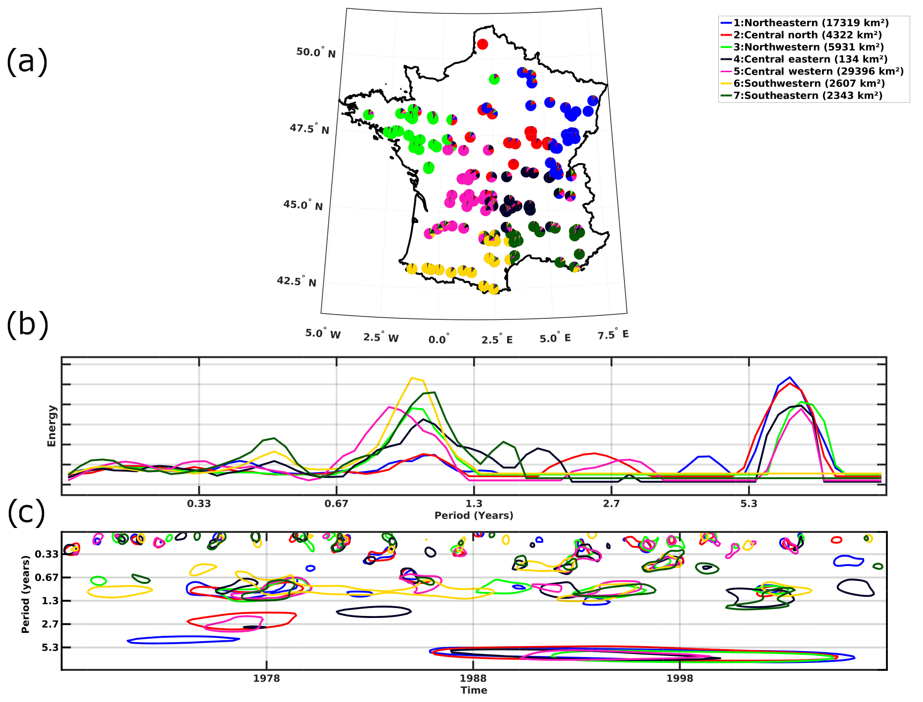
Figure 4 Clustering of precipitation time frequency variability in France. (a) Classification map of the watersheds. Pie chart slices show the three highest probability memberships. Pie charts denote fuzzy clustering memberships. (b) Global wavelet spectra of homogeneous regions. (c) Wavelet spectra of homogeneous regions. For clarity, only timescales and time locations that are 95 % statistically significant and with the largest variability are shown (colored circles).

3.1 Precipitation

3.1.1 Time frequency patterns

The following seven regions with homogeneous time frequency patterns are identified (Fig. 4a): northwestern (green), northeastern (blue), central north (red), central western (pink), central eastern (black), southwestern (yellow), and southeastern (dark green). Figure 4a shows that all watersheds converge toward singular clusters, meaning that all regions are highly coherent (i.e., pie charts in Fig. 4a show one dominant color).

In all regions, precipitation is varying at different timescales, ranging from intraseasonal to interannual scales (i.e., 2–8 years; Fig. 4b). Southwestern and southeastern regions are dominated by annual (1 year) variability, while their interannual variability (2–8 years) is low and the reverse for other regions. In addition, statistically significant areas in continuous wavelet spectra show that those timescales of variability are nonstationary (Fig. 4c), with temporal changes in terms of amplitude discriminating the different regions. For instance, southwestern regions are characterized by quasi-continuous significant annual variability until the late 1980s, while other watersheds show sparsely significant annual variability (Fig. 4c). Similarly, although there is significant interannual variability in all watersheds from the late 1980s, during this period, southwestern and southeastern regions do not show significant interannual variations (Fig. 4c). After removing the ≤1-year timescales (i.e., the seasonal cycle) focusing on interannual timescales, significant variability at 2- (southwestern) and 5-year (southwestern and southeastern) timescales emerge for the southern regions. The largest variations (i.e., colored circles) occur over shorter periods of time than in other regions (Fig. 5b).

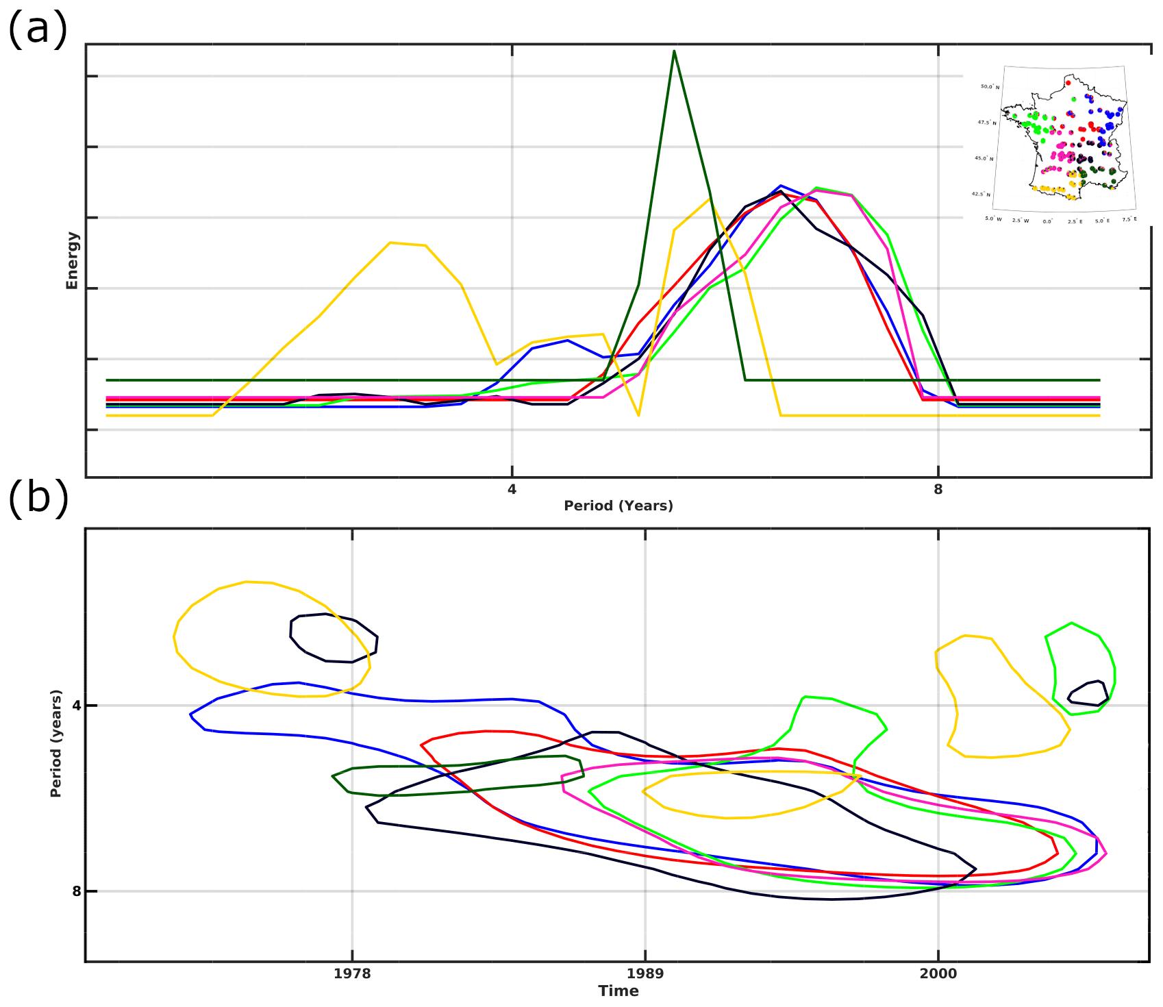
Figure 5 Interannual precipitation time frequency variability in France. (a) Global wavelet spectra of homogeneous regions. (b) Wavelet spectra of homogeneous regions. For clarity, only timescales and time locations that are 95 % statistically significant and with the largest variability are shown (colored circles).

In summary, different regions with coherent precipitation variability are identified and are characterized by three timescales of variability, i.e., intraseasonal, annual, and interannual. The amplitude of those timescales of variability, however, differs in time and over the French territory. Mediterranean regions (southwestern and southeastern) have comparatively weaker interannual variability as compared to annual timescales. The differences between regions are both dependent on the local expression of the climate forcing and watershed characteristics. Because those physical processes are interacting, studying cross-scale interactions in precipitation brings more insight on the dynamics behind the spectral characteristics of each region (Boé, 2013; Materia et al., 2021; Bellucci et al., 2015; Ardilouze et al., 2020).

Figure 6 Precipitation cross-scale interactions (95 % significance level). The driving timescale is on the horizontal axis and the driven on the vertical axis (i.e., the timescale where the x phase has a causal relationship with the phase/amplitude of the driven timescale y). The lower (upper) half of the graph, below (above) the diagonal, shows timescales acting on smaller (larger) timescales. (a) Phase–phase causality. (b) Phase–amplitude causality.

3.1.2 Cross-scale interactions

Figure 6 shows cross-scale interactions for each cluster of precipitation variability (see Fig. 4).

Northeastern, southeastern, north-central, northwestern, and central-eastern regions all show the phase of a 5–8-year variability driving the variability of smaller timescales (Fig. 6a; blue, dark green, red, green, and black; lower half of the graph). This cross-scale interaction is, however, more pronounced in the northeastern and southeastern regions (Fig. 6a). Similarly, eastern regions exclusively show 5–8 to 2–4-year interactions, while other regions show the self-interacting 5–8-year variability (Fig. 6a). The upper half of the graph, which refers to the higher frequency driving the lower-frequency variability, is populated by north-central, southeastern, northwestern, and northeastern regions (Fig. 6a; red, dark green, green and blue). The southeastern region shows cascade phase–phase interactions, (i.e., from 2–3 and 5–4 to 6–5 years; Fig. 6a, dark green). In addition, both southeastern and northwestern regions show mirror interactions with their lower-half counterparts, e.g., 5–6 to 4–5 years (Fig. 6a; dark green and green mirror patches about the diagonal). We also note that phase–phase interactions are very weak over the southwestern regions and absent in the central-western regions.

Phase–amplitude interactions are presented in Fig. 6b. The lower half of the graph, which refers to the lower frequency driving the higher-frequency variability, shows 5–8- to 2–4-year interactions for the western and north-central regions (Fig. 6b; pink, yellow, green, and red). The central-eastern regions are also showing the lower-frequency variability driving the higher-frequency variability but between 8- and 6-year variability (Fig. 6b). Notably, the northwestern region is the only one with cross-scale interactions driving the annual cycle (Fig. 6a; green). In the upper half of the graph, which refers to higher frequency driving lower-frequency variability, we only find north-central and northeastern regions showing 2–4- to 4- and 3–4- to 7–8-year phase–amplitude interactions (Fig. 6b; blue and red). Note that north-central, northeastern, and central-eastern regions show phase–amplitude and phase–phase interactions at very similar timescales (Fig. 6a and b; red, blue, and black), while timescales of phase–amplitude and phase–phase interactions do not match in central-western, northwestern, and southwestern regions (Fig. 6a and b; pink, green, and yellow). Regions to the east, thus, appear to have both phase–phase and phase–amplitude interactions at the same timescales, while western regions are more characterized by phase–amplitude interactions.

The precipitation cross-scale interactions can be of different forms, namely phase–phase, phase–amplitude, uni- or bi-directional, and from lower to higher timescales and vice versa. The presence of cross-scale interactions seems to be tied to specific spatial locations, suggesting different internal dynamics over the different regions of homogeneous precipitation variability. Interestingly, cross-scale interactions tend to converge toward specific timescales, notably 2–4 and 5–8 years, which were linked to ocean–atmosphere variability, such as the North Atlantic Oscillation, in previous hydroclimate studies over France (Feliks et al., 2011; Fritier et al., 2012; Dieppois et al., 2016; Massei et al., 2017). In addition, the presence of mirror interactions also indicate strong bidirectional negative feedback.

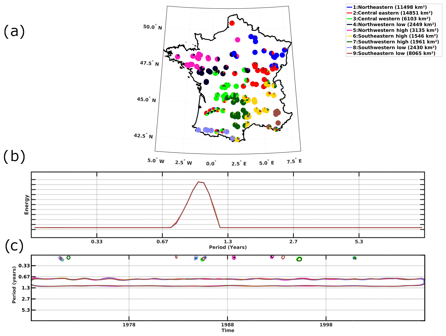
Figure 7 Clustering of temperature time frequency variability in France. (a) Classification map of the watersheds. Pie chart slices show the three highest probability memberships. (b) Global wavelet spectra of regions. (c) Wavelet spectra of homogeneous regions. For clarity, only timescales and time locations that are 95 % statistically significant and with the largest variability are shown (colored circles).

3.2 Temperature

3.2.1 Time frequency patterns

In temperature, the following nine regions with homogeneous time frequency patterns are identified (Fig. 7a): northwestern high (pink), northwestern low (black), northeastern (blue), central eastern (red), central western (green), southeastern high (yellow), southeastern low (brown), southwestern high (dark green), and southwestern low (purple). Fuzzy clustering shows that watersheds typically converge toward singular clusters, defining highly coherent regions (Fig. 7a). This is, however, not true for the central-western region, which is characterized by a mix of spectral characteristic defining other regions (see the red, green, black, yellow, and purple pie charts; Fig. 7a).

Using monthly data, temperature is primarily varying on an annual timescale, with very similar amplitudes for all regions (Fig. 7b and c). Since the dominant annual variability masks the other timescales, we use the annual time step to study interannual variability (Fig. 8a and b). Focusing on this interannual variability, significant temperature variations indeed emerge at 2–4- and 5–8-year timescales and show different timings and amplitudes over the different regions (Fig. 8a and b). All regions show 5–8-year variability, but, compared to northern regions, southern regions show significantly stronger variations on 2–4-year timescale (Fig. 8a). Similarly, while stronger 2–4-year variability occurs in the 1980s and 1990s in the southwestern low region, other regions show significant 2–4-year variability from the 2000s only (brown; Fig. 8b).

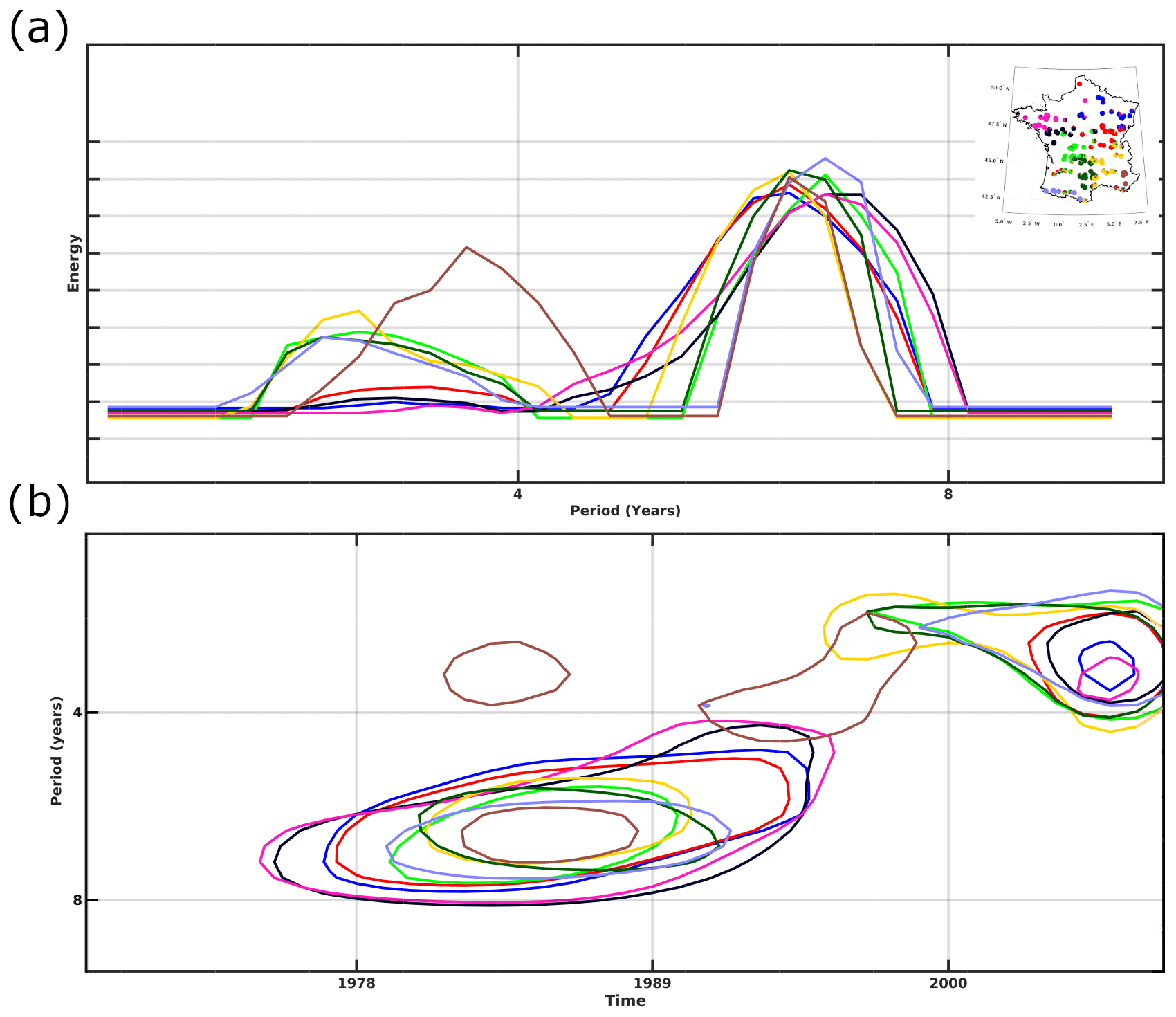
Figure 8 Interannual temperature time frequency variability in France. (a) Global wavelet spectra of homogeneous regions. (b) Wavelet spectra of homogeneous regions. For clarity, only timescales and time locations that are 95 % statistically significant and with the largest variability are shown (colored circles).

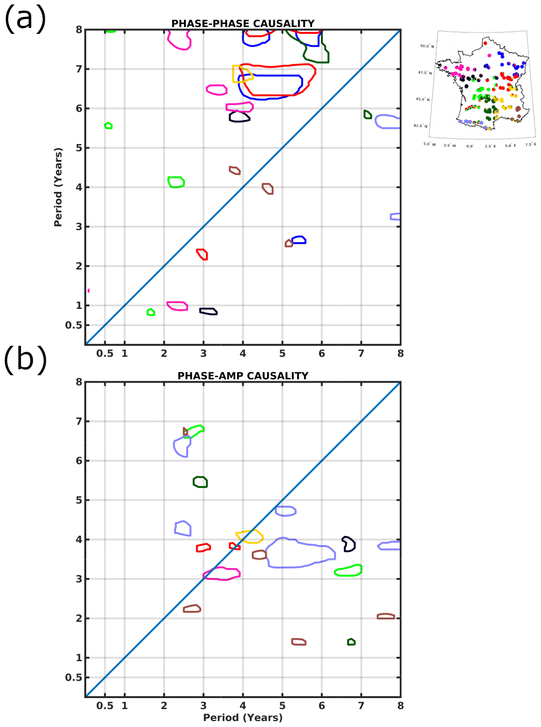
Figure 9 Temperature cross-scale interactions (95 % significance level). The driving timescale is on the horizontal axis and the driven on the vertical axis (i.e., the timescale x phase has a causal relationship with the phase/amplitude of the driven timescale y). Lower (upper) half of the graph, below (above) the diagonal, shows timescales acting on smaller (larger) timescales. (a) Phase–phase causality. (b) Phase–amplitude causality.

3.2.2 Cross-scale interactions

Figure 9 shows cross-scale interactions for each cluster of temperature variability identified in Fig. 8a.

For temperature, phase–phase interactions are mostly concentrated in the upper half of the graph, which refers to higher frequency modulating lower frequency (Fig. 9a). Notably, a 2–6- to 6–8-year phase–phase interaction appears more pronounced over northern regions (Fig. 9a; blue, red, pink, and black). The central-western region shows similar phase–phase interactions, but at 1–3- to 4–6-year timescales (Fig. 9a; green). In the lower half of the graph, which refers to lower frequency modulating higher frequency, interactions are found at very similar timescales, but at slightly higher frequency, for all regions (e.g., 2–5- to 1–4-year variability; Fig. 9a). Temperature in the southwestern low region, however, show slightly different characteristics with phase–phase interactions between lower and higher frequency occurring between 7–8- and 3–4- and 7–8- to 3–4-year variability (Fig. 9a; purple).

Temperature phase–amplitude interactions are mostly acting on the 3–4-year timescale for all regions (Fig. 9b). In particular, in temperature, more pronounced phase–amplitude interactions are found over the southwestern low region (Fig. 9b; purple), which is consistent with previous studies on phase–amplitude interactions in European temperature (Palus, 2014; Jajcay et al., 2016). Over southwestern regions, temperature, however, shows both 3–8- and 3–4- and 2–4- and 4–7-year phase–amplitude interactions (Fig. 9b; brown and purple). Furthermore, it should be noted that temperature variability interactions occur between very similar timescales over a number of regions (Fig. 9b; pink, red, yellow, and purple). According to Palus (2014), interactions between very similar timescales, or the same timescales, can only occur if, at least, two processes are present.

As for precipitation, in temperature, phase–phase and phase–amplitude cross-scale interactions are region dependent and can be uni- or bi-lateral. However, in temperature, most phase–phase interactions occur from higher- to lower-frequency variability, while phase–amplitude interactions tend to occur from lower- to higher-frequency variability. Similarly, while timescales of variability that are involved for phase–phase and phase–amplitude interactions are very similar in precipitation, they differ largely in temperature (Fig. 9b). This suggests that, in temperature, the processes driving phase–phase and phase–amplitude cross-scale interactions are different. It also suggests that the processes driving cross-scale interactions are different in temperature and in precipitation.

Figure 10 Clustering of discharge time frequency variability in France. (a) Classification map of the watersheds. Pie chart slices show the three highest probability memberships. (b) Global wavelet spectra of homogeneous regions. (c) Wavelet spectra of homogeneous regions. For clarity, only timescales and time locations that are 95 % statistically significant and with the largest variability are shown (colored circles).

3.3 Discharge

3.3.1 Time frequency patterns

The following six regions with homogeneous time frequency patterns are identified in discharge (Fig. 10a): northwestern (black), northeastern (blue), north central (red), central western (green), southeastern (yellow) and southwestern (pink). However, several watersheds, especially in the south, show memberships in multiple regions, suggesting lower spatial coherence in discharge than in precipitation and temperature. Lower spatial coherence, however, could mostly be explained by (i) mixing of solid and liquid precipitation in driving discharge variability in the Alps and (ii) the local heterogeneity of precipitation due to convective dynamics in the Pyrenees (Gottardi et al., 2008; Büntgen et al., 2008; Hermida et al., 2015). Nevertheless, the number of significant homogeneous regions is lower in discharge than in precipitation and temperature, and northern regions are particularly coherent.

Using monthly data, discharge is mainly varying on annual timescales, as determined through the global wavelet spectra (Fig. 10b). In addition, unlike other regions, southeastern watersheds show significant intraseasonal variability (Fig. 10b). Continuous wavelet spectra show that both annual and intraseasonal variability can be nonstationary, with temporal changes in terms of amplitude discriminating the different homogeneous regions of discharge variability (Fig. 10c). For instance, annual variability is only significant for specific periods in the southeastern watersheds, while other regions show quasi-continuous significant annual variability (Fig. 10c). Similarly, in the southeastern region, intraseasonal discharge variability sparsely appears significant from the 1980s, while they are absent in other regions (Fig. 10b).

Figure 11 Interannual discharge time frequency variability in France. (a) Global wavelet spectra of homogeneous regions. (b) Wavelet spectra of homogeneous regions. For clarity, only timescales and time locations that are 95 % statistically significant and with the largest variability are shown (colored circles).

After removing the seasonality, and focusing on interannual variability, northeastern watersheds stand out as having continuous significant interannual variability throughout the time series, with 4–5- and 5–8-year variability before and after the 1990s, respectively (Fig. 11b). Southeastern and southwestern regions also stand out, as they show 2–4-year variability in the mid-1970s and 2000s (Fig. 11b; yellow and pink). In addition, southeastern regions do not show significant variability in discharge at timescales greater than 4 years (Fig. 11a and b).

Different coherent regions are thus identified for discharge variability. In addition, these homogeneous regions correspond well with regions identified in precipitation and temperature variability. As in precipitation and temperature, those regions seem strongly impacted constrained temperature, and southern regions, which may appear more complex in term of climate and its link to land surface processes, appear much less spatially coherent in discharge.

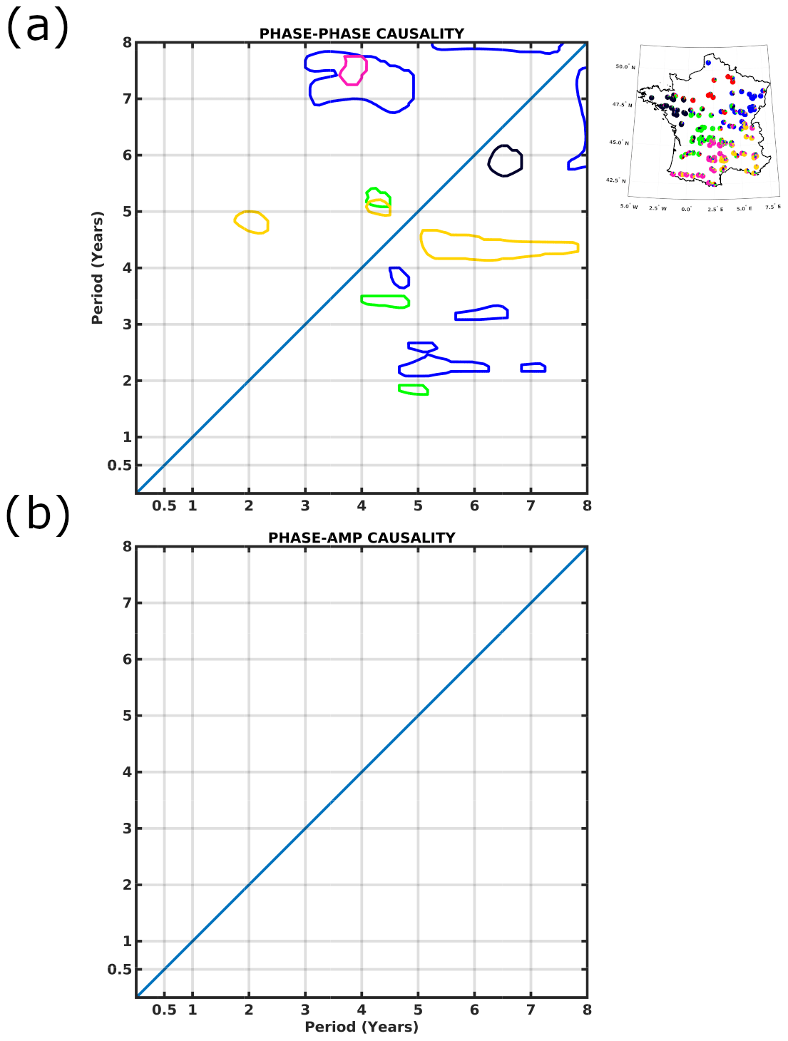
Figure 12 Discharge cross-scale interactions (95 % significance level). The driving timescale is on the horizontal axis and the driven on the vertical axis (i.e., the timescale x phase has a causal relationship with the phase/amplitude of the driven timescale y). Lower (upper) half of the graph, below (above) the diagonal, shows timescales acting on smaller (larger) timescales. (a) Phase–phase causality. (b) Phase–amplitude causality.

3.3.2 Cross-scale interactions

An important question concerning discharge cross-scale interactions is whether interactions found in either precipitation or temperature are also present in discharge. Phase–phase interactions that were found in precipitation are also identified in discharge, in particular over the northeastern, southeastern, and northwestern regions (blue, yellow, and black; Figs. 6a and 12a). Phase–phase interactions that were identified in temperature are much less evident (Figs. 9a and 12a). It should also be noted that many small patches, describing phase–phase interactions in precipitation and temperature, are systematically not transferred to discharge variability (Figs. 6a, 9a, 12a). Instead, discharge variability seems to exclusively preserve large patches of phase–phase interactions (Figs. 6a, 9a, 12a), suggesting that catchment properties are modulating the climatic signals (i.e., precipitation and temperature). Such filtering of climate signals is even more pronounced in certain regions, such as the north central, where phase–phase interactions are absent in discharge (Fig. 12a) but were identified in precipitation and temperature (Figs. 6a and 9a).

More importantly, there is no phase–amplitude interaction in discharge (Fig. 12b). This points out that watershed properties modulate the interacting processes in precipitation and temperature. Because our data set is mostly composed of low groundwater support, those modulations are unlikely to result from the water table, especially as phase–phase interactions are inherited from precipitation. In addition, further analysis at the Paris Austerlitz gauging station, which includes very large groundwater support, reveals the same absence of phase–amplitude interaction in discharge (not shown; Flipo et al., 2020). Possible explanations include the frequency partitioning of watershed compartments or integration process along the river network breaks any spatial connection and thus smooths out and flattens phase–amplitude interactions (Schuite et al., 2019).

Cross-scale interactions are only of phase–phase nature in discharge. All phase–phase interactions in discharge seem to be primarily related to precipitation, even though the strong correlations between rainfall and temperature makes it difficult to detect. However, differences between regions of homogeneous discharge variability are very similar to those detected in precipitation. Further work is, however, needed to understand why phase–amplitude cross-interactions are absent in discharge variability. Catchment properties appear to involve positive rather than negative feedback, thus resulting in a loss in phase–amplitude interactions.

4 Discussions and conclusions

4.1 Spatial variability of homogeneous hydroclimate variability in France

As recommended by Blöschl et al. (2019), characterizing the different scales of spatial and temporal variability, as well as their interactions, remains one of the most important challenges in hydrology. In this study, we unraveled homogeneous regions of hydroclimate variability in France, accounting for nonstationarity and nonlinearity, bringing additional information over previous, regime-based, classifications in France or elsewhere (Champeaux and Tamburini, 1996; Bower and Hannah, 2002; Sauquet et al., 2008; Snelder et al., 2009; Joly et al., 2010; Gudmundsson et al., 2011). This was achieved through a clustering analysis based on time frequency patterns of precipitation, temperature, and discharge variability over 152 watersheds. We then studied the spatiotemporal characteristics of each homogeneous region, including characteristic timescales of hydroclimate variability (i.e., precipitation, temperature, and discharge) and cross-scale interactions.

Our study reveals different coherent regions of precipitation, temperature and discharge variability. Yet, some watersheds are characterized by a mix of spectral characteristics from surrounding regions or regions with the same topographic characteristics. Those coherent regions are homogeneously distributed over France in precipitation and discharge but show larger discrepancies in term of spatial extension in temperature. According to previous clustering of hydroclimate variability over France, northern regions are more homogeneous than what was found here (Champeaux and Tamburini, 1996; Sauquet et al., 2008; Snelder et al., 2009; Joly et al., 2010) and show lower spatial coherence. In particular, here, we demonstrate that both the amplitude and timings of the different timescales of hydroclimate variability differentiate the regions, highlighting the need for accounting for nonstationary behavior in global to regional hydroclimate study. Overall, hydroclimate variability displays intraseasonal (<1 year), annual (1 year), and interannual (2–4 and 5–8 years) timescales. Our results, which were focused on the French territory, are therefore consistent with timescales of variability identified over the world's major rivers (Labat, 2006).

The timescales identified in this study have been shown to be important in climate processes, such as the North Atlantic Oscillation or the Gulf Stream front (Massei et al., 2007; Feliks et al., 2010; O'Reilly et al., 2017). Their interactions with watershed characteristics likely leads to their local expression with local processes, which play an important role in feedback mechanisms dampening or enhancing how the climate variability is expressed at the local scale (Haslinger et al., 2021; Materia et al., 2021; Bellucci et al., 2015).

4.2 Cross-scale interactions

Feedback mechanisms can occur between any physical processes of the hydroclimate system, and identifying or attributing the nature of these processes is an intractable issue using observational data. Nevertheless, we can use the mandatory conditions for cross-scale interactions to discuss the processes that are potentially at play (Fig. 3). In precipitation, cross-scale interactions involve lower-frequency timescales driving higher-frequency timescales. North Atlantic climate variability encompasses various processes, such as North Atlantic Oscillation or sea surface temperature anomalies, that drive climate variability (Feliks et al., 2010; O'Reilly et al., 2016). Thus, moisture advection from the North Atlantic area could potentially act as a positive feedback forcing. Moisture advection has indeed been shown to impact western Europe precipitation, especially in wintertime (Sun et al., 2020; O'Reilly et al., 2017). Zonal moisture advection is only forcing precipitation variability when the region is not affected by blocking weather regimes (Haslinger et al., 2019, 2021). Furthermore, vegetation, temperature and soil moisture, which are themselves interacting with each other, can act as a dampening forcing, thus dampening the precipitation. The precipitation–temperature, precipitation–soil moisture and precipitation–vegetation feedback have indeed been shown to reach a negative sign, depending on prior state of the soil (Liu et al., 2006; Berg et al., 2015; Liu et al., 2006). However, the sign of temperature–soil moisture–vegetation feedback on precipitation has been shown to be spatially dependent at the global scale. For instance, while temperature and soil moisture have large effects in western Europe, vegetation feedback is stronger and mostly of a positive sign in northern Europe (Woodward et al., 1998; Liu et al., 2006; Yang et al., 2018). In our results, the southeastern region shows interannual phase–phase interactions (Fig. 6a), which in contradiction with recent literature. For instance, in the Mediterranean region, Ardilouze et al. (2020) found no negative soil moisture precipitation feedback for interannual scales; however, the authors used two climate models to simulate soil moisture sensitivity to precipitation forcing and note that this variability is much larger in century-long reanalysis, such as NOAA's 20CR. For other regions, interannual negative soil moisture feedback was found by Boé (2013), while Sejas et al. (2014) found negative ocean–land temperature differences in precipitation feedback. Similar results were found in Bellucci et al. (2015), where interactions between compartments of the atmospheric circulation at intraseasonal timescale were found to produce significant interannual variations.

Interannual temperature variability is tied to both the soil state and atmospheric circulation, but that relation is location dependent. Large-scale patterns, such as the North Atlantic Oscillation, are shown to be source of both interannual precipitation and temperature variability, especially during wintertime, including for southwestern France (Pepin and Kidd, 2006; O'Reilly et al., 2016). At more local scales, sea surface temperature anomalies have been shown to interact with near-surface air temperature through sea–land heat exchanges regions (Lambert et al., 2011; Sejas et al., 2014; Zveryaev, 2015). Soil moisture and evapotranspiration demand can enhance or dampen near-surface temperature variability (Miralles et al., 2012; Materia et al., 2021). Here, in temperature, phase–phase interactions are particularly interesting because they arise from higher-frequency timescales driving lower-frequency timescales (Fig. 9a). As shown by Peters et al. (2004, 2007), higher-frequency processes can spread to lower-frequency ones by the means of intermediate timescale processes. High-frequency soil moisture enhancing lower-frequency large-scale circulation may explain temperature cross-scale interactions.

Regarding cross-scale interactions in discharge variability, the absence of phase–amplitude was particularly interesting. As our discharge data set is mostly composed of low groundwater support, the absence of phase–amplitude interactions is unlikely to result from the water table, especially as phase–phase interactions are inherited from precipitation. To test this hypothesis, we computed cross-scale interactions on the gauging station at Paris Austerlitz, which was not included in our original data set, as it shows large groundwater support and anthropogenic influence. Results at Paris Austerlitz are consistent with other regions and do not show any phase–amplitude interactions (not shown). As it has been shown that spatial heterogeneity (in the variable dynamics) favors cross-scale interactions, one possible explanation is that converging of runoff into the main drain cancels that spatial heterogeneity and, thus, phase–amplitude variability (Peters et al., 2007).

In this study, we interpreted cross-scale interactions based on the mandatory structure for such interactions to arise, identified interacting timescales, and compared cross-scale interactions in both precipitation, temperature, and discharge. Dedicated studies are needed to explore, in depth, the drivers of those interactions, as feedback mechanisms are complex, and likely different for each variable, even though phase–phase interactions in discharge clearly show the signature of those identified in precipitation.

4.3 Conclusion

Those findings allow for a better identification of climate-deterministic processes controlling hydroclimate variability, notably using cross-scale analysis, which could help in identifying more robust climate drivers. For instance, it is important to discriminate pure climate influence from climate–land processes interactions. This has large implications for seamless hydrological predictions based on climate information, as only some parts of the climate signals are transferred to discharge systems. Thus, causal cross-scale relationships could be used to inform and improve existing seasonal to multi-year seamless forecasting for hydrological variability, including extremes (e.g., flood and drought). Preliminary work in this direction was recently proposed by Jajcay et al. (2018), who developed a composite binning method enabling one to forecast a particular time series based on conditional phase of another. Similarly, it would be of crucial importance to determine whether hydrological models, which are commonly used in climate-impact assessments, are reproducing the filtering processes induced by the catchment properties and then identify those (Ducharne et al., 2020). Long-term hydroclimate variability only represents a fraction of the total variability; however, strong interactions between high- and low-frequency variations have been highlighted. Those interactions are both spatial and temporal (Feliks et al., 2016). Owing to the recent addition of long-term, high spatial resolution hydroclimate data sets (e.g., Fyre reconstructions; Devers et al., 2020, 2021), it is now possible to apply the clustering and cross-scale analyses to better characterize the effects that long-term hydroclimate variability (e.g., multi-decadal) has on smaller timescales. The methodology presented in this work can enable deeper analyses than those based on correlations, which may overlook some important hydroclimate processes.