Effects of spatial resolution of terrain models on modelled discharge and soil loss in Oaxaca, Mexico

The effect of the spatial resolution of digital terrain models (DTMs) on topography and soil erosion modelling is well documented for low resolutions. Nowadays, the availability of high spatial resolution DTMs from unmanned aerial vehicles (UAVs) opens new horizons for detailed assessment of soil erosion with hydrological models, but the effects of DTM resolution on model outputs at this scale have not been systematically tested. This study combines plot-scale soil erosion measurements, UAV-derived DTMs, and spatially explicit soil erosion modelling to select an appropriate spatial resolution based on allowable loss of information.

During 39 precipitation events, sediment and soil samples were collected on five bounded and unbounded plots and four land covers (forest, fallow, maize, and eroded bare land). Additional soil samples were collected across a 220 ha watershed to generate soil maps. Precipitation was collected by two rain gauges and vegetation was mapped. A total of two UAV campaigns over the watershed resulted in a 0.60 m spatial-resolution DTM used for resampling to 1, 2, 4, 8, and 15 m and a multispectral orthomosaic to generate a land cover map. The OpenLISEM model was calibrated at plot level at 1 m resolution and then extended to the watershed level at the different DTM resolutions.

Resampling the 1 m DTM to lower resolutions resulted in an overall reduction in slope. This reduction was driven by migration of pixels from higher to lower slope values; its magnitude was proportional to resolution. At the watershed outlet, 1 and 2 m resolution models exhibited the largest hydrograph and sedigraph peaks, total runoff, and soil loss; they proportionally decreased with resolution. Sedigraphs were more sensitive than hydrographs to spatial resolution, particularly at the highest resolutions. The highest-resolution models exhibited a wider range of predicted soil loss due to their larger number of pixels and steeper slopes. The proposed evaluation method was shown to be appropriate and transferable for soil erosion modelling studies, indicating that 4 m resolution (<5 % loss of slope information) was sufficient for describing soil erosion variability at the study site.

1 Introduction

The expansion of the agricultural frontier has been identified as being one of the factors driving the increase in global agricultural production (FAO, 2013), but this increase has a cost. Removal of natural vegetation due to agricultural expansion results in loss of soil, soil biota, organic matter, and nutrients, ultimately reducing the productivity of ecosystems (Palm et al., 2007). Up to 24 Pg (1 Pg = 1 billion Mg) of topsoil are lost annually and globally through land degradation (UNCCD, 2017), mainly due to soil erosion costing more than USD 40 billion in lost productivity (UNEP, 2012).

There are two main approaches to assessing soil erosion, i.e. measurement and estimation. Measurement is time and energy consuming and hence often limited to a small number of experimental plots (Wischmeier and Smith, 1978). Estimation, on the other hand, requires information about influencing factors (precipitation, soil properties, soil surface, and topography). To estimate erosion, two types of simulation models, empirical and physically based, are distinguished (Batista et al., 2019; Pandey et al., 2016). Physically based models such as OpenLISEM (Jetten, 2018) or LUCIA (Lippe et al., 2014) aim at capturing relevant processes from two-dimensional plots to three-dimensional landscapes and from minutes to days in temporal resolution.

Model input parameters can be measured in situ or in the laboratory or remotely sensed. At the landscape level, a cost-effective and reliable technique for data acquisition is remote sensing. In hydrologic and soil erosion modelling, required remote sensing data sets include topography (e.g. digital terrain model – DTM) and spectral imagery to derive land cover maps. Currently, the highest-resolution DEM (digital elevation model) sets, which are free and publicly available, are 30 m (i.e. Shuttle Radar Topography Mission, SRTM, and Advanced Spaceborne Thermal Emission and Reflection Radiometer, ASTER), with almost global coverage.

UAV (unmanned aerial vehicle) technology has been successfully applied in agriculture for crop health monitoring (Loladze et al., 2019), crop height estimation, vegetation segmentation (Hassanein et al., 2018), weed management (Castaldi et al., 2017), crop row detection (Comba et al., 2015), and crop phenology, among others, aiming at cost-effective, low environmental impact agriculture (Hassanein et al., 2018). Current UAV technology offers an increase in spatial resolution of spectral imagery products (tens of centimetres) compared to satellite data sets (tens of metres).

Hydrologic modelling of relatively large areas using high spatial-resolution DTMs often implies vast calculations, resulting in large modelling time and storage size. An option to reduce both is to resample to lower resolutions, finding a balance between well-represented topography and realistic modelled processes. Resampling of high-resolution DTMs to lower resolutions involves loss of information (Olson, 2007), and the magnitude of this loss depends on the heterogeneity of topography and geomorphology (Laso Bayas et al., 2015). Several studies mostly working with SRTM/ASTER and airborne lidar (Hoang et al., 2018; Olson, 2007; Wang et al., 2012; Wu et al., 2005) have shown that the spatial resolution of DTMs has a significant effect on maximum, mean, and standard deviation of elevation and slope; as resolution progressively decreases, so the ranges of elevation and slope narrow. This impacts hydrological (Hoang et al., 2018) and soil erosion modelling (Wu et al., 2005). The availability of high-resolution DTMs allows for the evaluation of the effects of different spatial resolutions on topographic characteristics and hydrologic and soil erosion modelling against measured high-resolution data. The present study pioneers the use of both high-resolution DTMs and multispectral imagery generated from a UAV at hundreds of hectares, combined with plot-scale measurements and OpenLISEM modelling, aiming to assess the effect of spatial resolution on modelled soil erosion.

The objectives of this study were to (a) assess the effect of DTM resolution on hydrologic and soil erosion modelling and (b) propose a method to identify an appropriate spatial resolution. To reach these objectives, the three tasks were as follows: (i) to calibrate/validate OpenLISEM at the plot level using a 1 m resolution DTM, (ii) to adjust the calibrated/validated parameters to the watershed level at the spatial resolution of five different DTMs (1, 2, 4, 8 and 15 m), and (iii) to identify an appropriate spatial resolution for modelling the study area.

2 Materials and methods

2.1 Description of the study area

Field data were collected in a 219.6 ha watershed known for severe erosion. The Cuauhtemoc watershed lies within Santa Catarina Tayata (SC Tayata) municipality in the Mixteca Alta region, Oaxaca, Mexico (Fig. 1), where serious soil erosion has been described as an “ecological disaster” (Guerrero-Arenas et al., 2010). The severity of soil erosion is presumably caused by highly erodible soils and inadequate land use/farming practices which have been in place since precolonial times (Palacio-Prieto et al., 2016).

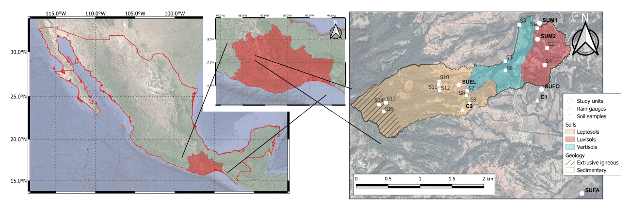
Figure 1 The Cuauhtemoc watershed (study units, rain gauges, soil samples, soil, and geology). Source: National Institute of Statistics and Geography (INEGI 2002, 2013).

The watershed area is dominated by silty and clayey continental sediments (Ferrusquia Villafranca, 1976) which form the highly erodible Yanhuitlán formation (Palacio-Prieto et al., 2016). Dominant reference soil groups in the watershed are (i) Leptosols, i.e. shallow soils formed by erosion, occupying the largest proportion, (ii) Vertisols, i.e. deep clayey soils, and (iii) Luvisols, i.e. soils with Bt horizon of clay illuviation and relatively high base saturation (INEGI, 2014; Fig. 1). The climate is temperate subhumid, with a mean annual temperature between 12 and 18 ^∘C and a rainy season from late June to late September (INEGI, 2008).

Land cover types within the watershed are representative of those at the municipality level, i.e. mainly mature natural forest, eroded bare land, cultivated area, and other covered areas (buildings, roads). A total of five soil erosion monitoring study units (SUs) represent the four main land covers (Fig. 1), namely forest (SUFO), eroded bare land (SUEL), maize cultivation on two different slopes and soil types (SUM1 and SUM2), and fallow (SUFA). The term study units includes bounded Wischmeier and Smith plots (4×22.1 m; Wischmeier and Smith, 1978) for SUFO and SUFA and unbounded microcatchments delineated by GPS for SUM1, SUM2, and SUEL.

The SUFO plot was installed on a steep slope (29 %) on a Luvisol, slightly outside the watershed under dense pine (Pinus sp.) and understorey shrub vegetation. The SUFA plot was installed on a former maize field fallowed in 2017. The plot was located on a 15 % slope on a Luvisol 1.7 km from the watershed as it had been installed prior to watershed delineation.

SUM1 and SUM2 microcatchments were located on 6 % and 12 % slopes and had an area of 1024 and 1061 m², respectively. Soil in SUM1 was less cohesive than in SUM2 (3 and 10 kPa, respectively). Both were mono-cropped with maize, of the local variety called Blanco, planted at 90×25 cm on 8 May 2017, and not weeded. The SUEL microcatchment had an area of 110.1 m², was located on a 13 % slope, had very low soil cohesion, and been bare for many years. Table 1 provides the study units' characteristics.

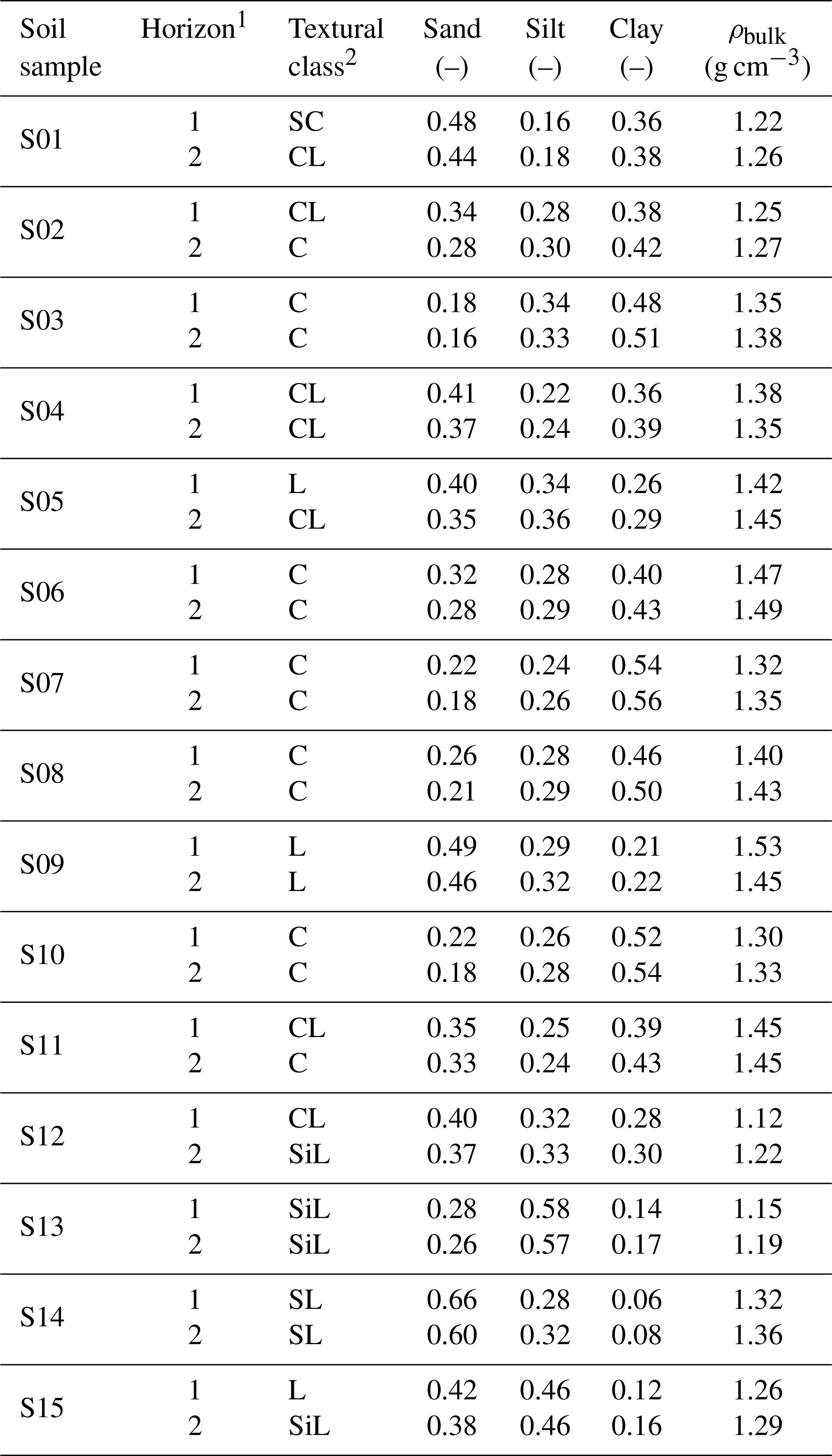
Table 1 Soil properties at the study units.

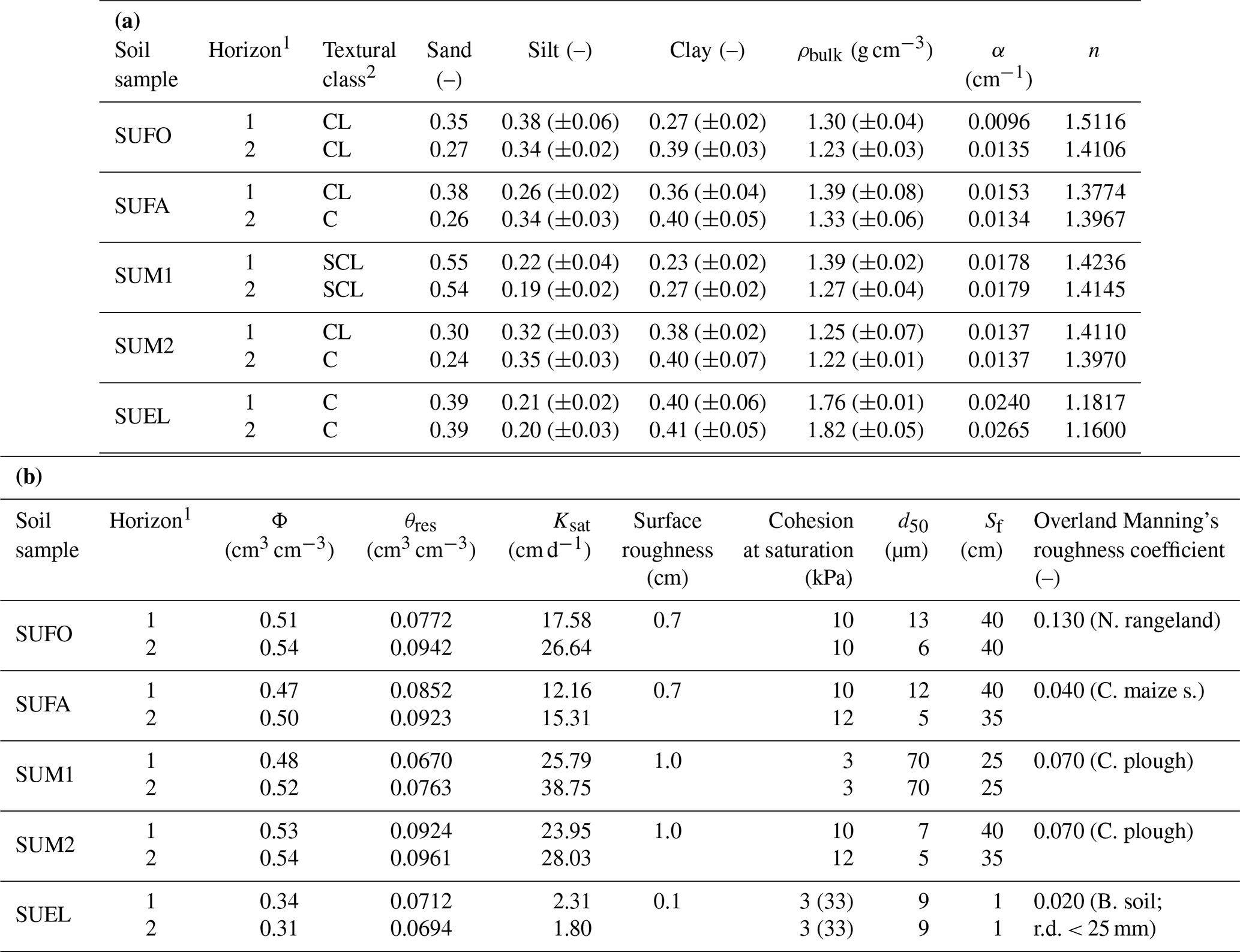
¹ Horizon 1 from 0–40 cm and horizon 2 from 40–100 cm; ² C – clay; CL – clay loam; SCL – sandy clay loam. Notes: (1) Sand, silt, and clay fractions and ρ_bulk were averages of the subsamples at 10 cm depth increments per horizon (soil properties/surface roughness in Sect. 2.2.2). (2) f, Van Genuchten parameters (α and n), Φ, θ_res, and K_sat were derived from Rosetta using texture and ρ_bulk as inputs. (3) Cohesion at saturation, S_f, and d₅₀ were derived from texture. (4) Surface roughness is the average of five vertical measurements (soil properties/surface roughness in Sect. 2.2). (5) Overland Manning's roughness coefficient was obtained by primary land use using the OpenLISEM documentation and user manual (Jetten, 2018).

2.2 Data collection and processing

2.2.1 Weather

In total, two automatic rain gauges were installed (Fig. 1), with C1 being a Decagon ECRN-100 connected to a Decagon Em50 data logger and C2 a Pessl iMETOS connected to a HOBO UA-003-64 logger. The volumetric resolution of both rain gauges was 0.2 mm, and the logging interval was set to 2 min. The collection period was from 14 May to 10 August 2017. For modelling, a precipitation event was defined as a minimum of 2.0 mm (Miralles et al., 2010), with a minimum hiatus of 60 min between events.

Global radiation, air temperature, and relative humidity at 10 min intervals were measured with a Davis weather station model Vantage Pro2 installed in the town of SC Tayata, 3 km north of the watershed. Daily global radiation was summed, while air temperature and relative humidity were averaged. Actual evaporation and transpiration were estimated based on the vegetation crop coefficient (K_C), exposed and vegetated soil fractions, and the reference crop evapotranspiration (ET₀), calculated using the Food and Agriculture Organization of the United Nations (FAO) Penman–Monteith equation (Allen et al., 1998).

2.2.2 Soil properties/surface roughness

One soil profile and two disturbed auger samples at 10 cm depth increments down to 100 cm were collected per study unit, in addition to 15 augers throughout the watershed (Fig. 1), based on the observation of soil surface characteristics and existing soil maps from INEGI. All samples were analysed for texture, volumetric (θ), and gravimetric (θ_m) soil moisture, bulk density (ρ_bulk), and stone surface cover. Derived soil properties were saturated hydraulic conductivity (K_sat), average suction at the wetting front (S_f), porosity (Φ), residual soil moisture (θ_res), and van Genuchten parameters (f, α, and n), cohesion, median particle diameter (d₅₀), and overland/channel Manning's roughness coefficient. Surface roughness was measured in the field. Early in the campaign, and for a brief period, volumetric soil moisture (θ) at 20 cm depth was measured at SUFO and SUFA to calibrate infiltration.

For profile description, two soil horizons were determined, namely 0–40 and 40–100 cm depth, given the OpenLISEM setting. Texture and volumetric soil moisture were averaged per sampling point and horizon. Soil texture was derived by the pipette method (Black, 1965; Palmer and Troeh, 1977). Gravimetric soil moisture was estimated by the difference between wet and oven-dried samples. Bulk density was calculated as proposed by Lal and Shukla (2004) and Miyazaki (2006).

Cohesion values were derived from textural classes based on Morgan et al. (1998). Median particle diameter was determined by using the 50th percentile in a distribution curve of cumulative particle size interpolating from proportions of texture classes of clay < 2 µm, silt 2–50 µm, and sand 50–2000 µm (Bittelli et al., 2015). Overland and channel Manning's roughness coefficients were derived from OpenLISEM documentation (Jetten, 2018). Aggregate stability, the median number of drops required to decrease the soil aggregate mass by 50 %, was model calibrated.

A set of three 0.9×0.9 m sampling squares was installed randomly on every study unit where surface roughness (centimetres) was determined as the average of five vertical measurements from the horizontal profile line to the soil surface at the beginning of the collection period (Lehrsch et al., 1988). As the National Institute of Statistics and Geography (INEGI)-based soil units contained a range of soil physical measurements, a soil reclassification was performed by merging both our own transect data and the INEGI soil map (Fig. 1), as described in Appendix A. The resulting map is shown in Fig. 7c.

2.2.3 Vegetation

Fraction of vegetation cover (fCover) and leaf area index (LAI) were derived from Sentinel-2 satellite images processed in Sen2-Agri version 2.0.1 (Defourny et al., 2019). In total, 11 images of bottom-of-atmosphere reflectance (L2A) between 24 April and 26 September 2017 were processed to generate fCover and LAI maps using a nonlinear regression model established by Weiss et al. (2002). Average values per study unit were plotted against the day of the year (DOY) and least squares polynomial regression equation fitted with NumPy 1.13.3 (Oliphant, 2006). Canopy water storage was estimated as a function of LAI, as proposed in OpenLISEM (Jetten, 2018). Vegetation height in SUM and SUFA was measured with a measuring tape as the average of all plants within sampling squares at 2-week intervals and interpolated with a least squares polynomial regression between sampling dates. In SUFO, a constant height of 12 m was visually estimated.

2.2.4 Sediment

One sediment collection station was installed at the outlet of each study unit, consisting of a 0.5 m high and 2.0 m wide L-shaped plastic sheet attached to the soil and wooden poles, to trap sediment. Sediments were processed the day after each precipitation event; ponding excess water was removed, and wet sediment was weighed to 0.5 kg precision. Above a minimum of 0.25 kg, small sediment amounts (250 to 1000 g) were collected in plastic bags. Above 3 kg of wet soil, one subsample of 100 g was taken from every impair sample number. Samples were oven-dried at 105 ^∘C until constant weight.

2.3 UAV flight campaign and imagery processing: digital terrain model (DTM) and multispectral imagery

The flight campaigns were carried out using a senseFly fixed-wing eBee plus, equipped with either a multispectral Parrot Sequoia camera, which acquired images in four wavelengths, namely green (550 nm and 40 nm full width at half maximum, FWHM), red (660 nm and 40 nm FWHM), red edge (735 nm and 10 nm FWHM), and near-infrared (790 nm and 40 nm FWHM), with a resolution of 1.2 MP, or an RGB camera, S.O.D.A., with a resolution of 20.0 MP. The two cameras were mounted separately, and each flight campaign was conducted with different cameras.

The first campaign was flown in April 2016, before the rainy season, acquiring images during sunny conditions, using the S.O.D.A. camera, to obtain the DTM while most agricultural areas were not cropped. The flight covered the entire SC Tayata municipality (39.2 km²), including the Cuauhtemoc watershed (2.20 km²), flying at 425 m above ground and acquiring images with 65 % lateral (side lap) and 75 % longitudinal (front lap) overlaps flying east–west, resulting in a ground resolution of approx. 0.12 m.

The second campaign was flown in early October 2017 during high vegetation cover to obtain a multispectral orthomosaic and derive a land cover classification. The flight, at 320 m above ground, acquired images with 60 % lateral and 80 % longitudinal overlaps flying east–west, resulting in a ground resolution of approx. 0.40 m.

For both flight campaigns, high-accuracy corrections of the geolocation data measured with the UAV global navigation satellite system (GNSS) were calculated in the post-processing stage using the position of a fixed, pre-established real-time kinematic (RTK) base station as a reference. Post-processing kinematic (PPK) correction was then implemented during imagery geotagging processing (Benassi et al., 2017; Forlani et al., 2018; Volpato et al., 2021).

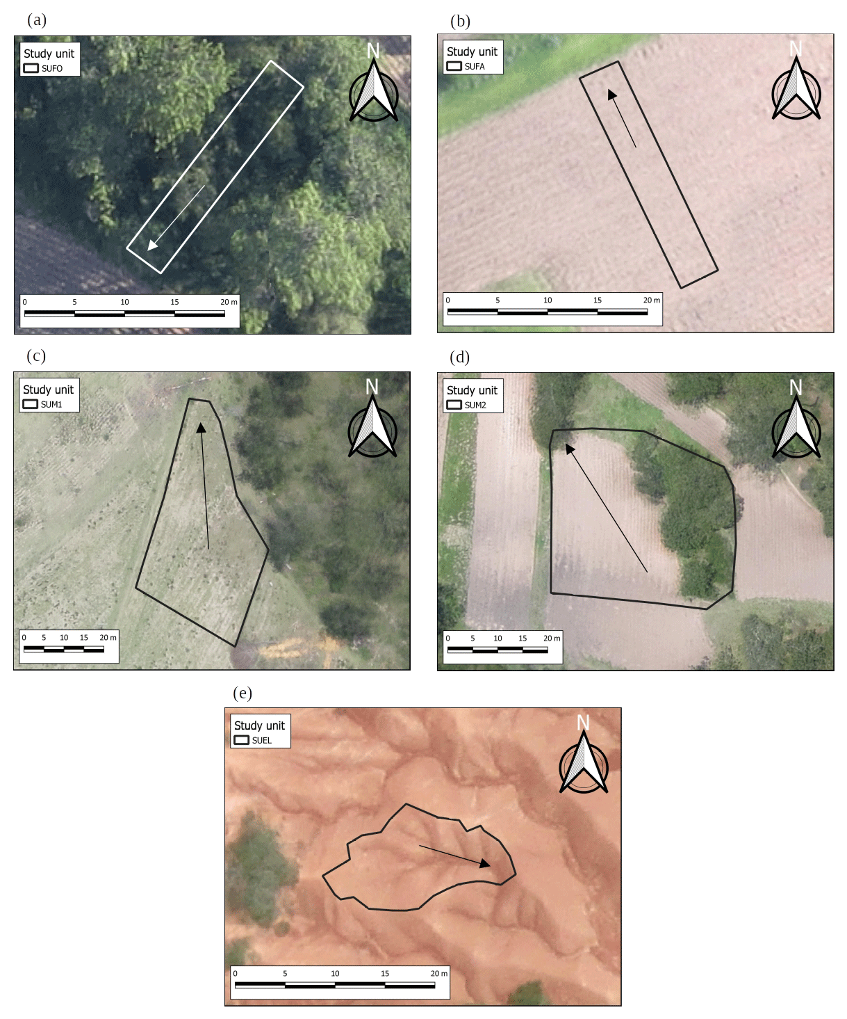
Figure 2 Study unit set-up with (a) SUFO (forest), (b) SUFA (fallow), (c) SUM1 (maize), (d) SUM2 (maize), and (e) SUEL (eroded bare land). Arrows indicate the main flow direction. Image source: 2016 UAV flight campaign.

UAV images were processed using Pix4Dmapper software (Pix4D, n.d.). Due to a reduction in spatial resolution when processing the DTM due to the Pix4D algorithm, which requires a minimum resolution of 5 times the ground sampling distance (GSD), DTM resolution was reduced to approx. 0.60 m.

2.4 DTM resampling and land cover classification

DTM resampling consisted of two steps, i.e. (i) resampling the original DTM with a spatial resolution of approx. 0.60 m to a baseline resolution of 1 m and (ii) resampling the baseline 1 m spatial resolution DTM to resolutions of 2, 4, 8, and 15 m. For resampling OSGeo4W shell, the Geospatial Data Abstraction Library (GDAL; GDAL/OGR contributors, 2020) and the average resampling method were used.

For land cover classification, the multispectral orthomosaic was processed using the Orfeo ToolBox plugin (Grizonnet et al., 2017) version 5.0.0 in QGIS 2.18.13 (QGIS Development Team, 2009). The land use classification procedure consisted of (i) creating in situ data polygons for training and validation using both the orthomosaic and ground observations, (ii) training the random forest algorithm, (iii) performing the classification of the orthomosaic using the derived trained model, and (iv) validating the previous classification using the validation polygons. The classification was performed with the classes of mature forest, eroded bare land, maize, and fallow, following the FAO's Land Cover Classification System (di Gregorio and Jansen, 1998). An additional class for permanent structures (i.e. roads) was added during post-classification.

Forest, maize, eroded bare land, fallow, and roads accounted for 60 %, 32 %, 4 %, 4 %, and <1 % of the watershed area, respectively. The overall accuracy index was 0.98, while the precision, recall, and F score of the first three land covers ranged from 0.71–1.0 and 0.86–1.0 to 0.80–1.0, respectively. Table B2 shows the confusion matrix of the classification.

2.5 Soil erosion modelling

We used OpenLISEM 4.96 (Jetten, 2018), a physically based, dynamic and distributed model that predicts event-based runoff and erosion via the following processes: overland and channel flow, detachment, deposition, sediment in transport, and soil loss. OpenLISEM was selected because (1) it is an open-source software (routines are transparent), (2) most input parameters are required in a grid format, i.e. respond to spatial resolution (our research question), and (3) its temporal resolution is user-defined, i.e. it can make full use of detailed rainfall measurements. A detailed description of processes simulated by OpenLISEM is given by Jetten (2018). Input parameters were either directly measured on site (on the ground or by UAV), derived using other software based on own measurements, or calibrated. Figure 3 provides an overview of data sources by OpenLISEM category.

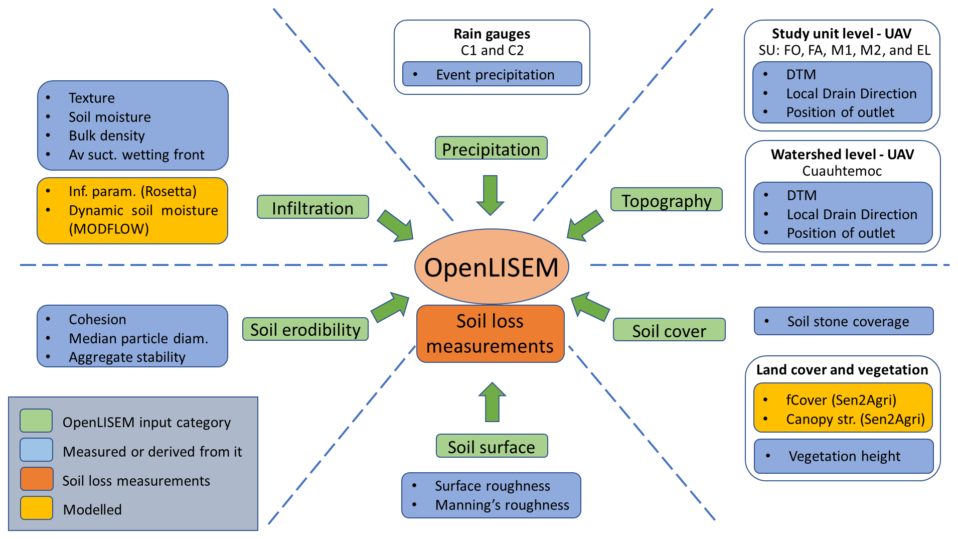
Figure 3 Overview of measured/derived input data used for modelling. Soil loss measurements on the ground were used for model validation.

Each study unit belonged to a single soil and land use class with homogeneous soil and vegetation properties (Fig. 2), while at the watershed scale, soil and land cover maps, including their soil and vegetation properties, differed with resolution.

For study unit parameterization, precipitation data were obtained from the nearest rain gauge and had a temporal resolution of 1 min. Slope, local drain direction, and outlet positions were calculated from the DTM.

Dynamic soil moisture and infiltration, used to determine initial soil moisture before measured events, were modelled using MODFLOW-2005 (Winston, 2009) and the package Unsaturated Flow Zone (UFZ) with a time step of 1 d, requiring soil physical properties, daily precipitation, and evapotranspiration as inputs. Initial values of K_sat and Φ were estimated for every soil type using Rosetta, a software to estimate soil hydraulic parameters (Schaap et al., 1998), which required measured soil texture and bulk density (ρ_bulk) as inputs (Fig. 3). The selected infiltration model in OpenLISEM (Green and Ampt) requires S_f, which was derived from texture, according to Rawls et al. (1983). To reduce computation time, we stopped event simulations once 95 % of the runoff had reached the outlet. The reason was to set sediment in transport ∼ 0, and Soil_loss ∼  Detachment – |Deposition|.

Calibration/validation of water balance components followed a two-step procedure: (1) infiltration was estimated in MODFLOW, using K_sat, and the infiltration $/$ precipitation ratio was computed for the collection period; (2) infiltration was then calibrated/validated in OpenLISEM using K_sat against the ratio of infiltration $/$ precipitation found in the first step. The events were split into two-thirds for calibration and one-third for validation.

Sediment balance components were calibrated and validated with soil cohesion and d₅₀, selected out of eight parameters after a sensitivity analysis. Collected sediment was compared against modelled Soil_loss per event and study unit. Again, two-thirds of the events were used for calibration and one-third for validation. Tables B4 and B5 show the final parameterization per land cover, soil type, and channel. To evaluate model performance at the study unit level, the root mean square error (RMSE), coefficient of determination (CD), and model efficiency (EF) were computed as proposed by Loague and Green (1991).

Our model scenarios consisted of watershed-level map sets at resolutions of 1, 2, 4, 8, and 15 m. An additional map of channels per resolution was created based on the local drain direction, assuming that a channel initiates when it accumulates 1 ha of area upstream. Assigned values of channel width/depth, Manning's roughness coefficient, cohesion, and K_sat were typical of channels in mountainous headwaters. Figure 4 shows a flowchart of upscaling from the study unit to the watershed level, starting with calibration/validation of water and sediment balance components at the study unit level.

Figure 4 Process of upscaling from study unit to watershed level.

Afterwards, the DTM was resampled to the different spatial resolutions, followed by the creation of slope, local drain direction, and outlet maps. All spatially explicit soil and vegetation maps were subsequently produced for each resolution.

To assess the effects of different spatial resolution on hydrological and soil erosion, modelling results were compared in two categories, namely (i) event hydrographs (litres per second; hereafter L s⁻¹) and sedigraphs (kilograms per minute; hereafter kg min⁻¹) at the watershed outlet using three distinctive precipitation magnitudes, i.e. low (2.6 mm), mid (8.4 mm), and high (23.0 mm), based on the distribution of all the events during the collection period and cumulative sediment yield during the collection period; and (ii) watershed-wide and land-cover-wide spatially distributed cumulative soil loss (megagrams per hectare) during the collection period.

3 Results and discussion

3.1 Data collection and processing – variables for model parameterization

3.1.1 Weather

Sums of event precipitation during the collection period (14 May to 10 August 2017) in C1 (n=37) and C2 (n=38) were 428.4 and 460.4 mm, respectively, during 39 rain events. The minimum, mean, and maximum of event precipitation were 2.2, 11.6, and 35.4 mm at C1 and 2.2, 12.1, and 36.2 mm at C2, respectively. The minimum, mean, and max of the total global radiation were 6.20, 15.71, and 24.21 MJ m⁻² d⁻¹, respectively. Mean air temperature and relative humidity were 18.9 ^∘C and 82.1 %, respectively. Maximum and minimum air temperature were 31.2 and 7.9 ^∘C, respectively. Assuming the 2017 rainy season followed the distribution of the long-term normal precipitation in Mexico's Hydro-Administrative Region V (Table B1), the precipitation in 2017 was between 8 % and 15 % lower than in the long term (1981–2010).

3.1.2 Soil properties/surface roughness

Among topsoil properties, texture in the study units (USDA – Soil Science Division Staff, 2017) was clay loam in SUFO, SUFA, and SUM2, sandy clay loam in SUM1, and clay in SUEL. Average bulk densities ranged between 1.22 and 1.39 g cm⁻³, except for SUEL (1.76 to 1.82 g cm⁻³), which was characterized by highly compacted to consolidated material. K_sat ranged between 12 and 26 cm d⁻¹, except in SUEL where it was 2 cm d⁻¹ (Table 1). Figure 7c and Table A2, respectively, show the reclassified soil map and a summary of soil properties after reclassification.

3.1.3 Vegetation

In SUFO, soil cover (fCover) detected by Sentinel-2 (only photosynthetically active vegetation) was constant at ∼0.5. In SUFA, cover in mid-May started at 0.17, reaching a maximum of 0.57 by the end of July and decreasing thereafter. SUM1 and SUM2 were averaged in one land use (SUM) in which cover in mid-May started at 0.04, reaching a maximum of 0.65 by the end of the collection period. Over time, canopy water storage from Sentinel-2 LAI data followed a similar pattern to soil cover. Largest values were estimated in SUM (2.43 mm), followed by SUFA (1.44 mm) and the coniferous SUFO (1.60 mm) (Table B3). Vegetation height was constantly 12 m in SUFO. SUM1 and SUM2 reached a maximum of 2.1 m and SUFA of 0.15 m towards the end of the season.

3.1.4 Sediment

Sediment yield was highly variable both in occurrence and magnitude amongst study units. During the collection period there were 0, 1, 6, 22, and 24 events that produced >250 g of sediment in SUFO, SUFA, SUM1, SUM2, and SUEL, respectively (the latter being shown in Fig. 5).

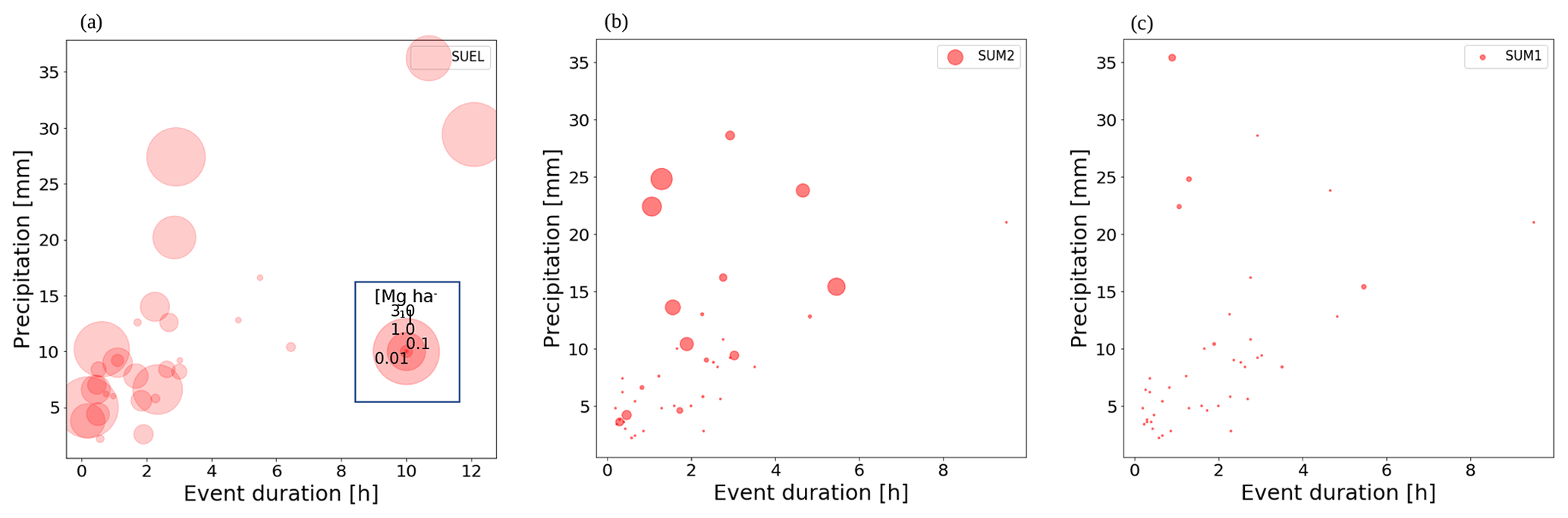
Figure 5 Event-based sediment yield (Mg ha⁻¹ per event) in relation to rainfall amount and duration in (a) SUEL, (b) SUM2, and (c) SUM1.

For most combinations of event intensities, sediment yield in SUEL (max. 2.99 Mg ha⁻¹ per event) was by far the largest, corresponding to rain gauge C2. Likewise, sediment yield in SUM2 (max. 0.32 Mg ha⁻¹ per event) was generally larger than in SUM1 (max. 0.04 Mg ha⁻¹ per event), corresponding to rain gauge C1.

Total erosion during the collection period was 19.1, 1.5, and 0.1 Mg ha⁻¹ at SUEL, SUM2, and SUM1, respectively. Considering the annual historical precipitation, these figures could be 31.0, 2.0, and 0.2 Mg ha⁻¹ yr⁻¹, respectively. SUEL was amongst the largest values globally (Pimentel and Kounang, 2007; Panagos et al., 2015) and locally (SEMARNAT, 2008). SUM2 was moderate to high, while SUM1 were in the null to slight category, according to Pimentel and Kounang (1998) and SEMARNAT (Secretariat of Environment and Natural Resources; 2008). SUFO and SUFA (≪1 Mg ha⁻¹) were in the null category. Table B6 shows a summary of the collected sediment.

3.2 UAV flight campaign and imagery processing

3.2.1 Study unit level: set-up, DTM, and slope

The probability density function (PDF) of slopes at the study units (Fig. 6) was extracted from the DTM of the 2016 UAV flight campaign. SUFO exhibited the largest proportion of steep pixels (mean of 0.29 m m⁻¹), followed by SUFA (0.15 m m⁻¹), SUEL (0.13 m m⁻¹), SUM2 (0.12 m m⁻¹), and SUM1 (0.06 m m⁻¹). SUFO was located near the watershed divide with steep slopes. SUFA, SUEL, and SUM2 were located between ridges and flat agricultural areas and SUM1 in a typical flat agricultural area (Fig. 7d).

Figure 6 Probability density function (PDF) of slope of study units based on UAV data.

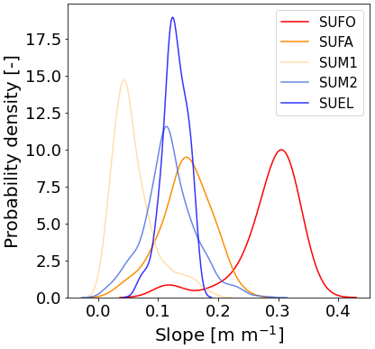
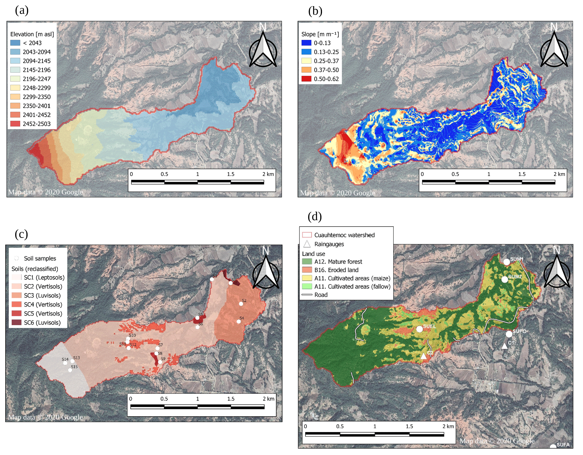
Figure 7 (a) Elevation, (b) slope, (c) reclassified soil map, and (d) land cover classification of the Cuauhtemoc watershed.

3.2.2 Watershed level: DTM and slope

The Cuauhtemoc watershed DTM and slope at 1 m spatial resolution are shown in Fig. 7. Maximum elevation was 2503 m a.s.l. (above sea level) in the southwest, and minimum elevation was 2043 m a.s.l. in the northeast at the watershed outlet. The east–west extension was approx. 3.6 km. The relief is diverse, with >20 % of the watershed area having slopes > 0.2 (Fig. 8b). Steeper slopes were found in the southwest and along most of the divide, and there were moderate to lower slopes towards the middle and northeastern parts of the watershed.

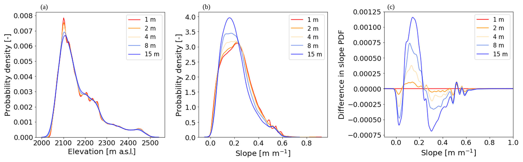
Figure 8 Probability density functions (PDFs) of resampled (a) elevation, (b) slope, and (c) difference of slopes between 1 m and other resolutions of the Cuauhtemoc watershed.

3.2.3 DTM resampling

Resampling to lower resolutions smoothened the peak elevation (in the range from 2175 to 2275 m a.s.l.; Fig. 8a) and slope values (in the range from 0.45 to 0.65 m m⁻¹; Fig. 8b).

The difference in slope PDF between 1 m and the resampled lower resolutions (Fig. 8c) shows a frequency reduction (negative sign in Fig. 8c) at both extremes (between 0 to 0.06 m m⁻¹ and 0.25 to 0.65 m m⁻¹) and a frequency increase in the mid range (from 0.06 to 0.25 m m⁻¹), and such a difference increased with decreasing resolution. In other words, the downgrading caused a migration of pixels from the lower and upper end regions to the middle region. Differences (areas below or above the curve) in slope PDF are shown in Table 2.

Table 2 Difference in slope PDF between 1 m and lower resolutions.

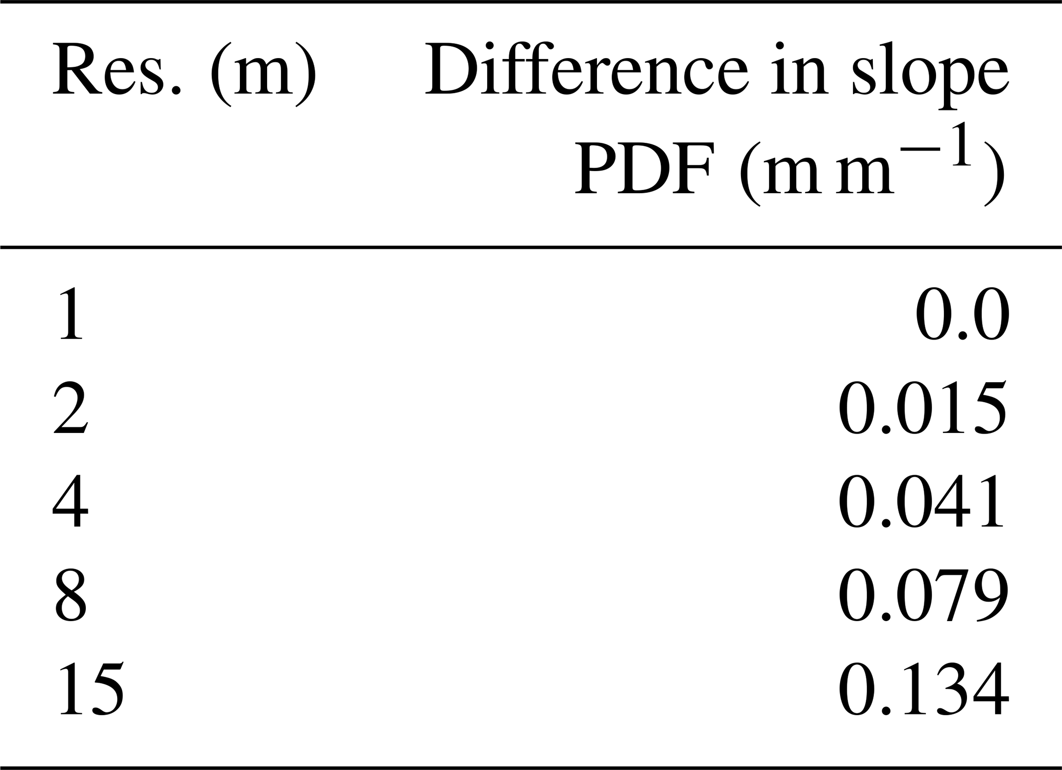
The largest difference, 0.134, corresponds to the 15 m resolution, and it reduced proportionally until 0.015, corresponding to the 2 m resolution. The mean slope decreased with resolution (0.227, 0.225, 0.221, 0.216, and 0.207 m m⁻¹ in decreasing order from 1 to 15 m resolutions), which has also been observed in other studies. Olson (2007) found, for a topographically diverse watershed in Minnesota, USA, that the slope's PDF aggressively shifted to a smaller magnitude when comparing a 2 m (peak of the PDF at 74^∘) lidar-generated digital elevation model (DEM) and a 30 m (peak of the PDF at 8^∘) DEM. Wang et al. (2012) found, for six study areas in China with contrasting topographical reliefs, that the mean slope was proportionally reduced as resolution decreased when comparing 10, 25, 50, and 100 m DEM. The authors also found that the reduction was larger in more (25 to 15^∘) than in less diverse topographies (10 to 7^∘).

Wu et al. (2005), working on a watershed in Virginia, USA, found that mean slope length and steepness factor (LS; nondimensional) of the Revised Universal Soil Loss Equation (RUSLE), which summarize the effect of topography on erosion, was proportionally reduced from 5.8 to 2.9 as resolution decreased when comparing 10, 30, 60, 100, 150, 200, and 250 m DEM. Finally, Hoang et al. (2018), working on a watershed in New York, USA, found that mean slope was proportionally reduced from 0.16 to 0.13 m m⁻¹ as resolution decreased when comparing much higher-resolution DEMs, i.e. 1, 3, 10, and 30 m.

Amongst these studies, variation in slopes can be attributed to at least two factors, namely range of spatial resolutions (1–250 m) and degree of topographical diversity (from highly diverse mountainous regions to less diverse, mostly flat, agricultural regions) across the studies.

When comparing the difference in slope (or slope-related parameters) between the highest and lowest resolution and the range of spatial resolutions, the difference tends to decrease when the highest resolution tends to 1 m and the lowest resolution is close to approx. 30 m but not coarser. In Hoang et al. (2018), the difference in slope between the highest (1 m) and lowest resolution (30 m) was about 0.2. On the other end, in Wu et al. (2005), the difference in the slope length and steepness (LS) factor between the highest (10 m) and lowest resolution (250 m) was about 0.5. In our study, the difference in slope between the highest (1 m) and lowest resolution (15 m) was 0.13, which was lower than in Hoang et al. (2018), probably due to the lower resolution (30 m) of their lowest resolution as compared to our study (15 m) or to differences in topographic diversity amongst the two study areas.

This trend suggests that, independently of topographical diversity, a small difference is achievable with resolutions much coarser than 1 m, given that the resolution of the base data set is at least 1 m. This difference has implications for the selection of an appropriate spatial resolution in hydrological and soil erosion modelling, as discussed later in this study.

3.3 Soil erosion modelling at the study unit level

Early campaign soil moisture measurements in SUFO and SUFA at 20 cm depth were used to calibrate infiltration in MODFLOW. Model performance at SUFO and SUFA were CD = 0.93 and 0.03, EF = 0.92 and −28.68, and RMSE = 1.91 and 1.57, respectively. Better performance at SUFO was probably due to a wider range of measurements (0.26–0.31 θ) as opposed to the narrow range/short period at SUFA (0.341–0.343 θ), which made it unsuitable for calibration, as shown by the poor model performance at SUFA, but rather a small RMSE. A reduction in the range 15 %–25 % of initial values of K_sat (Table 1) calculated with Rosetta was required for calibration of infiltration. For the remaining study units, reductions in initial K_sat values in this range were applied.

As a second step, the ratio infiltration/precipitation obtained from MODFLOW was used for infiltration calibration in OpenLISEM. A reduction in the range 0.6 %–1.3 % of MODFLOW values of K_sat (Table 1) was required for calibration. Grum et al. (2017) achieved good agreement (Nash–Sutcliffe efficiency – NSE > 0.6) between observed and predicted runoff by modifying K_sat in the range 0.2 %–7 % of the estimated K_sat of Hessel et al. (2006) by 0.8 %–3.6 % (NSE > 0.5) and of de Barros et al. (2014) by 5 % (NSE > 0.6). This suggests that the model overpredicts infiltration when parametrizing K_sat values in normal ranges. Possible causes are that the infiltration routine in the model's structure requires some tuning or that processes other than the ones considered in the model are relevant (i.e. sealing or crusting of the soil surface).

Figure 9 shows observed and predicted sediment yield at SUM2 and SUEL during calibration and validation. For SUM1, only six rain events produced >250 g of sediments.

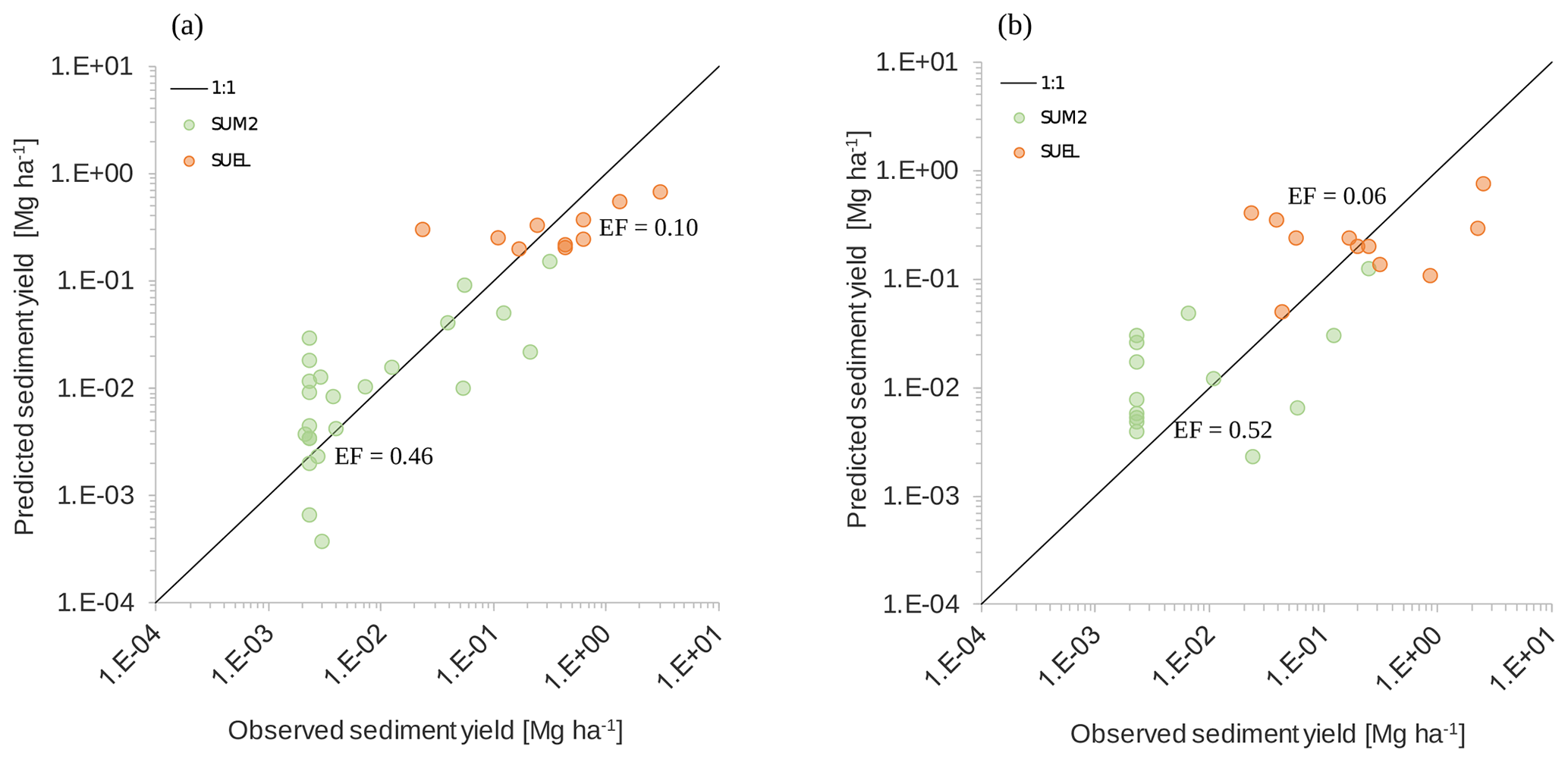
Figure 9 (a) Calibration and (b) validation of sediment yield at the study units SUM2 and SUEL.

The best model performance in SUM2 and SUEL was achieved by modifying soil cohesion in the range 10³–10⁴ and d₅₀ in the range 10¹–10⁴ of the measured/estimated values (Table 1). Calibration and validation parameters were as follows: for SUM2 – EF = 0.46 and 0.52, CD = 3.95 and 4.12, and RMSE = 154 and 133; for SUEL – EF = 0.10 and 0.06, CD = 4.54 and 5.06, and RMSE = 114 and 137. Parameters for SUFO, SUFA, and SUM1 were non-acceptable under modelling criteria. The reason for this was the narrow range of observed values (sediment yield ≤ 1 Mg ha⁻¹). OpenLISEM realistically predicted soil erosion in highly erodible soils (SUEL) and low to mild slopes (SUEL/SUM2). On the other hand, it had limitations in predicting soil erosion in highly cohesive soils (SUFO/SUFA), high slope terrains (SUFO), and low cohesive soils in combination with low slopes (SUM1; results not shown).

The below-mentioned studies calibrated sediment yield with soil cohesion and d₅₀. Grum et al. (2017) achieved a good model fit (R²>0.5; n=27) for sediment yield by modifying soil cohesion by 10⁴ and d₅₀ by 10³. Similarly, de Barros et al. (2014) achieved a good agreement for some events (NSE > 0.5; n=5) modifying soil cohesion by 10⁴. In both studies, the model generally overpredicted erosion. Calibration of sediment balance components in these studies was challenging, since the model performed satisfactorily for some events but poorly for others. The authors unanimously assumed that certain processes may not be adequately represented in the model. In these studies, model calibration was done either per event (Grum et al., 2017) or per class of events (de Barros et al., 2014); that is, different values of selected calibration parameters were selected for every event or class of events. In our study, we calibrated the selected parameters using a single value for all events because we wanted to isolate the effect of different spatial resolutions, and to achieve this, all the other parameters had to remain constant.

OpenLISEM performance was satisfactory for SUM2 and SUEL given the fact that its final parametrization, as mentioned above, evenly distributes over- and underestimated predictions which, over the collection period, averages observed erosion. Tables B4 and B5 list OpenLISEM parameters and calibrated values at the watershed level.

3.4 Soil erosion modelling at the watershed level with different spatial resolutions

For scenario modelling, watershed simulations with a distributed model based exclusively on plot data would not be good practice without additional downstream sampling points for validation. However, the main goal of our study was to determine the relative effect of DTM resolutions without validation to absolute values. Maps of model input parameters are shown in Fig. B1.

3.4.1 Modelled discharge and sediment yield at the watershed outlet

Event hydrograph (L s⁻¹) and sedigraph (kg min⁻¹) at the watershed outlet for three selected events with low, medium, and high-precipitation events are shown in Fig. 10.

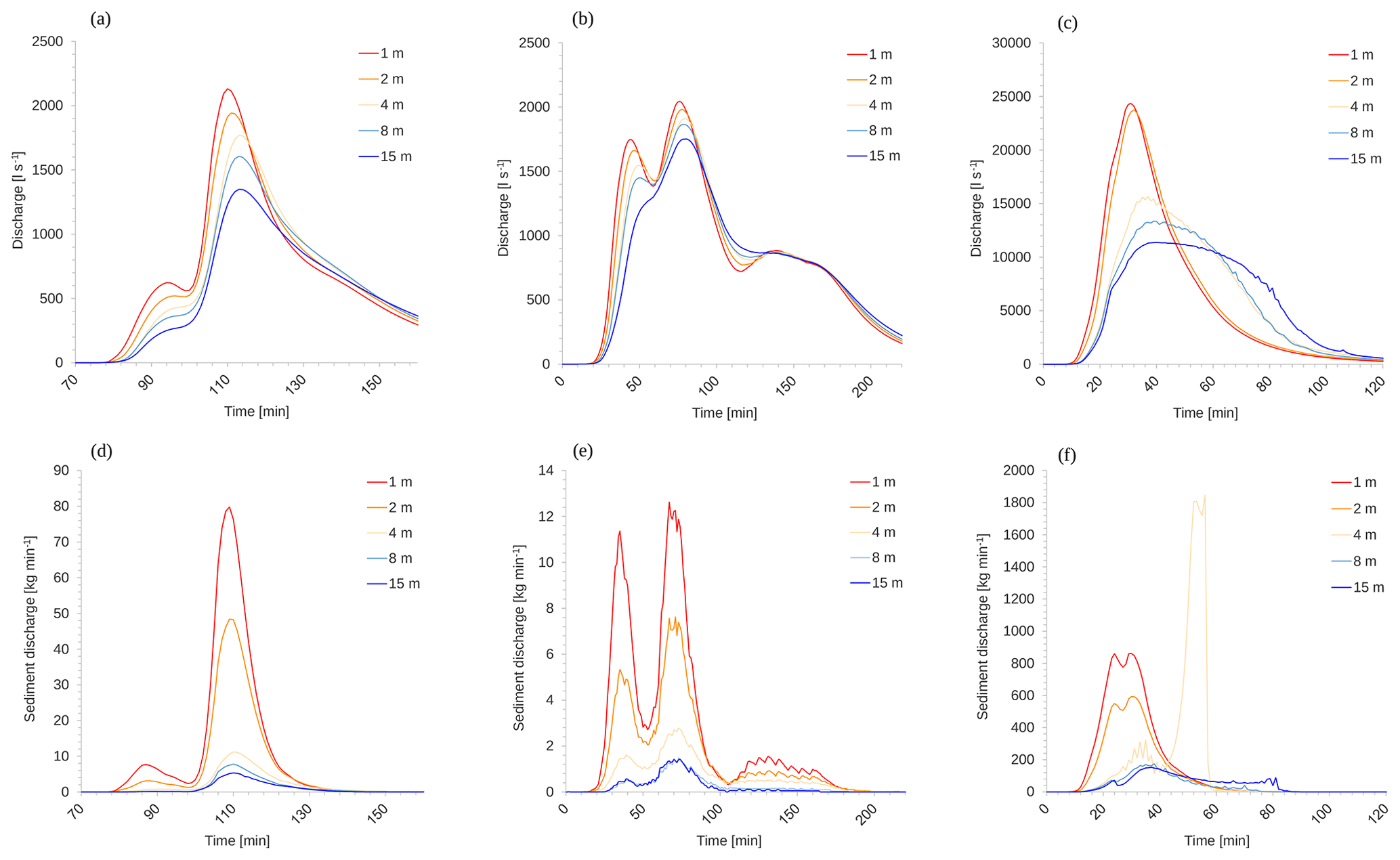
Figure 10 Hydrographs (a–c) and sedigraphs (d–f) at the watershed outlet at low- (2.6 mm; a, d), medium- (8.4 mm; b, e), and high-precipitation (23.0 mm; c, f) events. Note the different scaling of the x and y axes across the figures.

Hydrographs and sedigraphs differed significantly across resolutions with a trend in that the largest peak values occurred at the highest resolution and decreased with resolution (Fig. 10). Discharge at all three events started earlier (rising limb) and at a higher rate the higher the resolution was, while this ranking was reversed towards the end of the falling limb. The low- and mid-precipitation events exhibited a characteristic double peak (bimodal) hydrograph at 1 m resolution, which was gradually smoothened, shifting to one peak (unimodal) at lower resolutions.

Relative differences between peak discharge of the highest and lowest resolutions were not proportional across magnitudes of precipitation. While the highest peak at 15 m resolution was about 60 % and 40 % to that of 1 m resolution in the low- and high-precipitation events, respectively, this ratio was about 80 % in the mid-precipitation event, suggesting a significant influence of rainfall intensity. Total runoff (area under the hydrograph) was 4.51, 4.44, 4.26, 4.07, and 3.78×10³ m³ in the low-precipitation event, 11.78, 11.74, 11.56, 11.34, and 10.95×10³ m³ in the mid-precipitation event, and 44.24, 44.19, 43.64, 40.83, and 42.14×10³ m³ in the high-precipitation event in the 1, 2, 4, 8, and 15 m resolutions, respectively. The ratio runoff_15 m $/$ runoff_1 m was 0.84, 0.93, and 0.95 for the low-, mid-, and high-precipitation events, respectively.

Hessel et al. (2006) observed that at low temporal resolution (15 min) the model did not predict bimodal hydrographs and attributed this to smoothened rainfall intensities. Grum et al. (2017) assumed that asynchronous rainfall distribution in the watershed (three rain gauges in ∼12 km²) was overriding temporal discharge peaks. In contrast, de Barros et al. (2014) reported a good prediction even for multimodal hydrographs and attributed this performance, amongst others, to the high spatial discretization of parameters. Our model time step of 1 min was not limiting for detecting bimodal discharge patterns and thus allowed us to explore the effects of spatial resolution on temporal discharge patterns.

Sedigraphs, as a product of discharge and sediment concentration, exhibited larger differences across resolutions than hydrographs. Rising limbs started much earlier and rates of sediment discharge were larger in the 1 and 2 m resolution as compared to the remaining resolutions and to their hydrographs. At the same time, bimodal patterns were much more pronounced than in hydrographs. Total sediment yield was 0.98, 0.63, 0.19, 0.12, and 0.09 Mg in the low-precipitation event, 0.53, 0.33, 0.14, 0.06, and 0.05 Mg in the medium-precipitation event, and 18.28, 12.63, 18.76, 4.24, and 5.21 Mg in the high-precipitation event in the 1, 2, 4, 8, and 15 m resolutions, respectively. The ratio sediment yield_15 m $/$ sediment yield_1 m was 0.09, 0.09, and 0.29 for the low-, medium-, and high-precipitation events, respectively.

Sedigraphs imposed more challenge in achieving a good fit between predicted and observed values. However, sedigraphs were more sensitive than hydrographs to spatial resolution (lower ratios sediment yield_15 m $/$ sediment yield_1 m than runoff_15 m $/$ runoff_1 m). This sensitivity, particularly in the three highest resolutions (Fig. 10d–f), provides an opportunity for studies aiming at detailed sedigraphs.

The difference in event sediment yield between the 1 m and the remaining resolutions fluctuates from close to 0 up to ∼1 order of magnitude as event precipitation increases (Fig. 11). Cumulative sediment yield at the outlet during the collection period was 191.9, 128.4, 38.1, and 39.7 Mg in the 1, 2, 8, and 15 m resolutions. In the 4 m resolution, four excessively large events (one of them in Fig. 10f) drove the cumulative sediment yield to an unmatched 440.9 Mg. The four extreme sediment yield events occurred during high-precipitation events, even though the hydrograph (Fig. 10c) followed an intermediate trend between resolutions. This suggests that OpenLISEM's numerical routine for sediment balance finds an unexpected combination of values when processing the 4 m resolution in combination with high-precipitation events.

Figure 11 Event sediment yield (SY) at watershed outlet across resolutions.

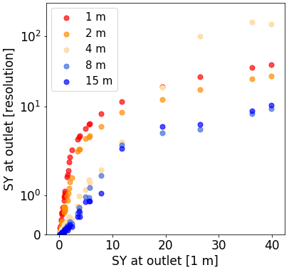
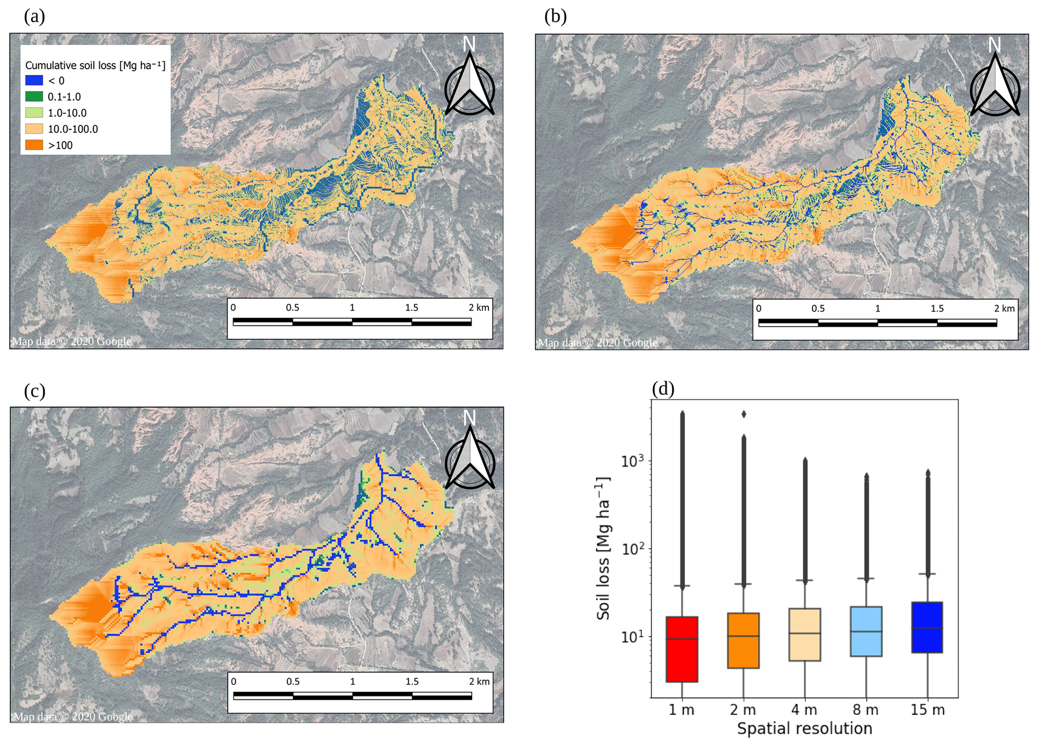
Figure 12 Cumulative soil loss (Mg ha⁻¹) during the collection period at (a) 1 m, (b) 4 m, and (c) 15 m resolution and (d) box plot per resolution.

3.4.2 Spatial distribution of soil loss in the watershed

Spatial distribution of cumulative soil loss during the study period for three selected spatial resolutions and a box plot of its distribution per land use are shown in Fig. 12.

Watershed-wide median soil loss (Fig. 12d) increased from 9.2 to 10.2 Mg ha⁻¹ from 1 to 15 m resolution. The proportional shifting upwards of the quartiles as resolution decreased (Fig. 12d) might be due to a combination of number of pixels and, hence, pixel diversity. In this study, the highest-resolution map (1 m) had 225 times (15²) more pixels than the lowest-resolution map (15 m), following a quadratic behaviour. The highest-resolution map (1 m) contained much higher diversity of values (e.g. soil loss) due to 2.196×10⁶ px than a lowest-resolution map (15 m) with 0.009×10⁶ px. This diversity of pixels widened the distribution of the highest-resolution map, while narrowing it in the lowest-resolution map. The fact that the quartiles shifted downwards as resolution increased may be due to the effect of a larger number of pixels with low slope (Fig. 8b and in the range 0 to 0.06 m m⁻¹) which translated to low soil loss. On the other hand, Fig. 12d also shows that the highest soil loss values in particular areas were obtained at the highest resolution (highest variation) as expected due to higher slopes in some pixels.

Independently of spatial resolution, along the watershed we found hotspots of soil loss in some areas in the southwestern end, in some areas along the watershed divide (typical high slope areas; Fig. 7b), and in the eroded bare land (Fig. 7c; SC4 – highly erodible soil). Likewise, negligible soil loss occurred where the slope was lower (Fig. 7b), e.g. on agricultural terraces in the middle of the watershed. Setting aside the eroded bare land, there appeared to be a good correlation between slope (Fig. 7b) and soil loss (Fig. 12), which underlines the well-known influence of slope on flow velocity and net soil transport. Hessel et al. (2006) also report similar erosion patterns (although of different magnitude) between the predicted soil loss map from the model and a soil erosion assessment map based on a survey conducted in the same rainy season, suggesting the ability of OpenLISEM to adequately capture spatial patterns of erosion.

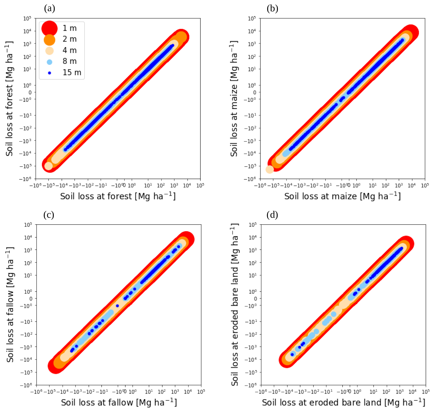
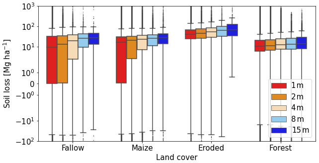
Figure 13 Cumulative soil loss (Mg ha⁻¹) of (a) forest, (b) maize, (c) fallow, and (d) eroded bare land cover across resolutions.

Land cover wise (Fig. 13a–d), the range of soil loss tended to decrease with resolution as depicted by the envelope of values from the highest to the subsequent lower resolutions. Another characteristic was the loss of continuity in values as resolution decreased; while 1 and 2 m resolution showed continuity between the highest and lowest soil loss value in all resolutions, 4 m showed quasi-continuity, 8 m showed continuity in forest and maize but not in fallow and eroded bare land, while 15 m showed discontinuity in all land cover except forest. This characteristic is most probably due to pixel diversity discussed earlier, given the land cover area proportions in the watershed, i.e. 60 %, 32 %, 4 %, and 4 % corresponding to forest, maize, fallow, and eroded bare land, respectively.

Resolutions of 1 and 2 m for maize and fallow (Fig. B2) exhibited a larger share of pixels in the vicinity of low soil loss (≤5 Mg ha⁻¹) as compared to the remaining resolutions and land covers. On the other end, 8 and 15 m resolutions at all land uses exhibited a larger share of pixels in the upper range (≥10 Mg ha⁻¹). A key message is that transition zones between agricultural lands (e.g. maize and fallow) and forest/eroded bare land represent candidate areas for preventive action. In this context, Koomson et al. (2020) highlighted the importance of critical slope length to control soil erosion. Moreover, corrective actions can also be promoted by locating and estimating erosion hotspots within the region and encouraging land use interventions to change eroded bare land back to agricultural land/forest.

The fact that higher-resolution sets did not exhibit larger overall soil loss (Fig. 12), even though exhibiting larger sediment yield at the watershed outlet (Fig. 11) may appear contradictory, but we propose two explanations. One argument is the contribution of pixels with extreme values to the overall sediment regime. Extreme soil loss (Fig. 12d) in the 1, 2, 4, 8, and 15 m resolution ranged from ∼40 to ∼3500, ∼2000, ∼1000, ∼700, and ∼800 Mg ha⁻¹, respectively. In our study, extreme values contributed with large quantities to the watershed sediment, and their effect was larger in the higher resolutions due to their largest pixel diversity. In other words, despite pixel area, much more extreme pixels with higher magnitudes of soil loss in the higher-resolution maps contributed overall more sediment to the watershed.

The second argument is the effect of both slope and density of the fluvial system on the time of concentration and hence on the watershed's sediment delivery ratio (SDR) which is the ratio sediment yield/gross sediment production. The time of concentration (time needed for water to flow from the most remote point in the watershed to the outlet) and the SDR are directly proportional to resolution; the higher the resolution, the higher the slope, and the higher density of the fluvial system (more channels, as they are more clearly defined). For instance, the highest resolution (1 m) with its higher slope (Fig. 8b) promotes faster flow velocities, and its denser fluvial system (results not shown) promotes a more efficient transport system, reducing the time of concentration. Hence, both larger sediment inputs and shorter times of concentration experienced by higher-resolution sets exhibit a larger sediment yield (Fig. 10) as compared to their lower-resolution counterparts.

3.5 Selection of an appropriate spatial resolution

Selection of an appropriate resolution in spatially distributed modelling depends, amongst others, on the spatio-temporal resolution of the process to be modelled. In soil erosion modelling, deposition is dependent on a detailed representation of both the slope and fluvial system since these define the flow velocity and path to the outlet, respectively. Detachment on the other hand is considered spatially independent since precipitation is assumed to be homogeneously distributed within the area represented by a rain gauge. An appropriate representation of both processes, however, depends on a high temporal resolution of precipitation and runoff. In this study, the temporal resolution was 1 min, which provided the highest possible temporal resolution in the LImburg Soil Erosion Model (OpenLISEM; millimetres per minute; hereafter mm min⁻¹), coming closest to field conditions. Our purpose for choosing this time step was to focus on aspects of spatial resolution. For scenario modelling exercises, temporal resolution may be reduced to economize computing power. The study area was heterogeneous in topography, with more than 20 % of the area exhibiting slopes > 0.2 (Figs. 7b and 8b). As such, slope maps were selected as an evaluation parameter given the findings of previous sections regarding DTM resampling, i.e. slope magnitude and distribution dependence on resolution.

The loss of information as a consequence of resampling is expressed by the difference in slope PDF (Table 1) between the highest resolution (1 m in our study) and the remaining resolutions, which can be interpreted as a deviation from reality, if we define the highest resolution as the reality. In this study, we set the borderline between acceptable and unacceptable deviation from reality at 5 % (i.e. 0.05). The highest resolution that fulfilled this criterion was 4 m.

Zhang and Montgomery (1994) studied the effect of DEM resolution on hydrological simulations in two catchments in the western USA. They report that the 10 m resolution provided a substantial improvement over 30 and 90 m resolutions, while 2 and 4 m provided only marginal improvement over the 10 m resolution. They suggested the 10 m resolution as a compromise between detail and computer storage volume. Wu et al. (2005) suggested that the best resolution may not necessarily be the highest resolution, but that spatial variability ought to be adequately represented.

Hoang et al. (2018) reported that 10 m resolution was the most appropriate in their study, since it provided a good representation of the landscape and was a compromise between too much detail in higher resolutions and lost information in coarser resolutions. Hessel et al. (2006) mentioned that a 20 m resolution was insufficient in their erosion modelling exercise, given complex land use patterns occurring at small scales not captured by the resolution. On the other end, de Barros et al. (2014), working with a 5 m resolution, mentioned that amongst the reasons for a good performance of OpenLISEM in predicting runoff was the high spatial discretization of the surface.

The above-mentioned studies, with their particular topographies, conclude that a spatial resolution of around 10 m may comprise a balance between a sufficiently detailed topography and allowable computational indicators (e.g. storage volume and modelling time). The diverse topography in our study area required a further increase in resolution to 4 m to stay within the 5 % deviation slope criteria chosen.

4 Conclusions

This study explored some of the effects that differences in spatial resolution have on the modelling of hydrographs and sedigraphs at the outlet from different events predicted by a spatially distributed soil erosion model in a topographically diverse ∼2.2 km² tropical watershed in southeastern Mexico. Furthermore, we explored the effects on the spatial distribution of soil loss during a period of ∼3 months in the 2017 rainy season.

The resampling resolution of DTM changed slope, with consequences for water residence time in the watershed (hydrograph) further influencing sediment transport and concentration in runoff (sedigraph). Effects on soil loss were most pronounced where the change in slope was most significant. A high-resolution map implies more pixels and, hence, higher diversity of values than a low-resolution map covering the same area. The higher the diversity of soil loss values, the more influence on overall sediment regime in a watershed. The results of this study allowed us to conclude the following.

Event-wise calibration of water balance components in OpenLISEM was more flexible and provided far better results than the calibration of sediment balance components. Calibration of sediment balance components achieved a better model fit in low-cohesion/highly erodible soils than in high-cohesion/low erodible soils. Model fit was also better for low to mild slope/low flow velocity compared to steep slopes/high flow velocity.

At the watershed outlet, the highest resolutions (i.e. 1 and 2 m) exhibited the largest hydrograph and sedigraph peaks, total runoff, and total soil loss, while these variables proportionally decreased with resolution. Sedigraphs were more sensitive than hydrographs to spatial resolution, particularly at the highest resolutions. Spatially distributed soil loss prediction fluctuated within a desirably narrow range across resolutions. The two highest resolutions exhibited a broader range of predicted soil loss due to their larger quantity of pixels and wider diversity of slopes, while slope proportionally decreased with resolution.

Resampling the DTM of a topographically diverse terrain from a fine resolution (1 m) to lower resolutions implied loss of information and a reduction in slope. This reduction was driven by the migration of pixels from the upper end (higher slope values) to lower values (the middle region), and its magnitude was proportional to resolution. There was also a less sensitive migration of pixels from the lower end (lower slope values) to higher values (the middle region); however, it was insufficient to overcome the effect of the first-mentioned migration.

The criterion for the selection of an appropriate spatial resolution was based on the evaluation of loss of information (5 % max) due to resampling as compared to the highest available resolution. The 4 m resolution proved to be sufficient for describing soil erosion at the studied area.

Appendix A: Soil reclassification

A summary of soil properties at the study units and at the 15 sampling locations is shown in Tables 1 (main text) and A1. The INEGI soil map (Fig. 1) was amended to include three more classes, based on the soil properties at the study units plus the sampling locations. It was clear that the boundary between Leptosols and Vertisols was located between samples S12 and S13, coinciding with the boundary between extrusive igneous and sedimentary rocks, which was verified with a transect around the area, so it was decided to assign the boundary between SC1 (Leptosols) and SC2 (Vertisols) to match the one between igneous and sedimentary rocks.

Within SC2, 10 samples were taken ranging between clay (S03, S06, S07, S08, and S10), clay loam (S11 and S12), and loam texture (S05 and S09). SUEL also had clay texture but differed from the clay group in its higher ρ_bulk (Table 1). SC2 soil properties matched average clay group properties, while two new soil types were created within SC2, i.e. SC5, whose soil properties were set to those of the average loam group, and SC4, whose soil properties were set to those of SUEL whose extension matched the eroded bare land area. Samples S11 and S12 were not considered in the reclassification because their properties differed from both clay and loam groups.

Within SC3 (Luvisols), six samples were taken and ranged between clay loam (SUM2, S02, S04, and SUFO) and sandy clay loam (S01 and SUM1). SC3 soil properties were set to those of SUM2. Within SC2 and SC3, one additional class was defined (SC6), for which the soil properties were set to those of SUM1. A summary of the soil properties after reclassification is shown in Table A2.

Table A1 Soil properties at transect points.

¹ Horizon 1 from 0–40 cm and horizon 2 from 40–100 cm; ² L – loam; C – clay; CL – clay loam; SCL – sandy clay loam; SiL – silt loam; SL – sandy loam; SC – sandy clay. Note: sand, silt, and clay fractions and ρ_bulk were the averages of the subsamples at 10 cm depth increments per horizon (soil properties/surface roughness in Sect. 2.2.2).

Table A2 Soil properties per soil class in Cuauhtemoc watershed.

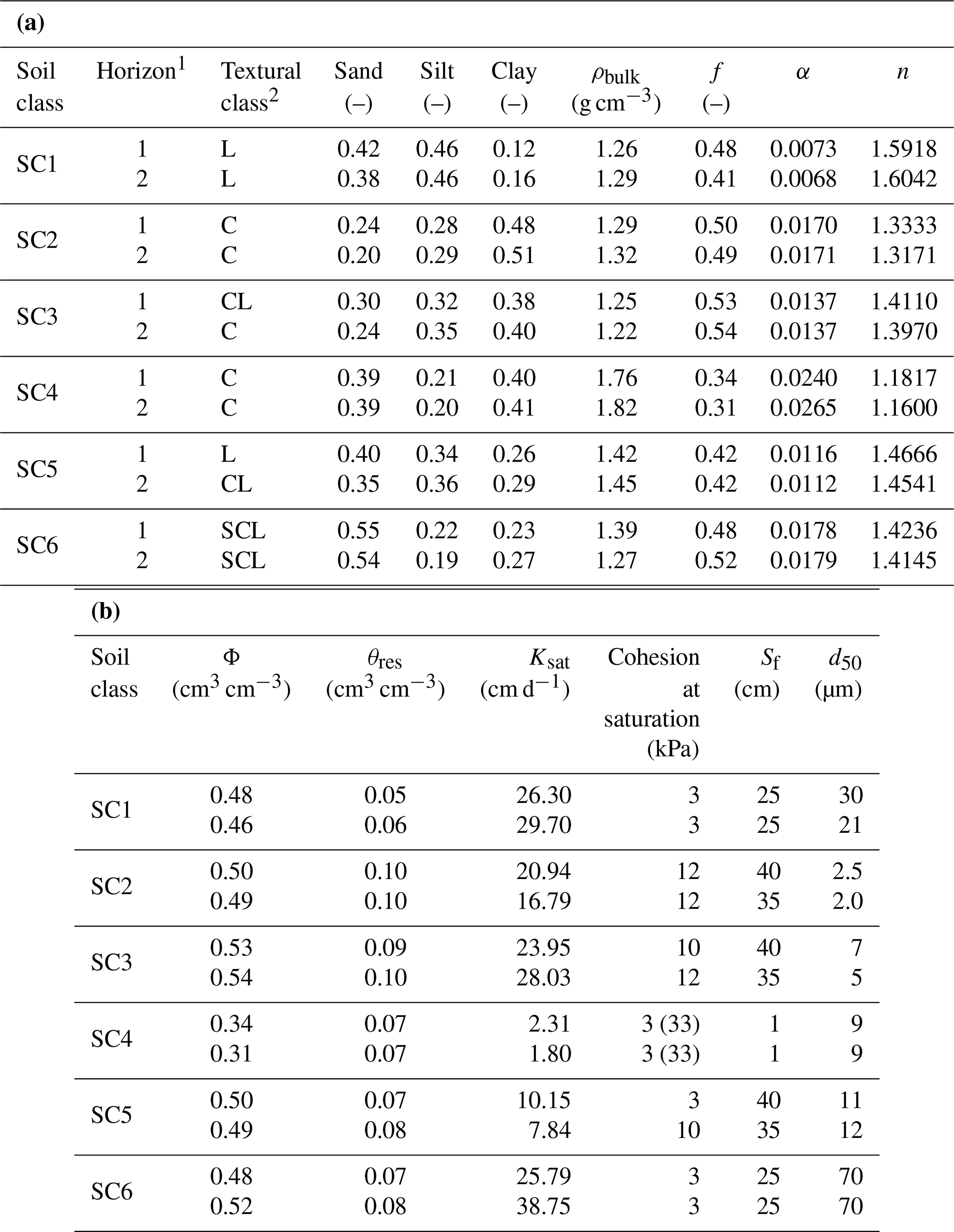
¹ Horizon 1 from 0–40 cm and horizon 2 from 40–100 cm; ² L – loam; C – Clay; CL – clay loam; SCL – sandy clay loam. Notes: (1) Sand and silt fractions and ρ_bulk were the average of the selected soil samples (soil profile and augers) within each soil class. (2) Clay fraction was calculated from sand and silt fractions. (3) f, Van Genuchten parameters (α and n), Φ, θ_res, and K_sat were derived from Rosetta, using texture and ρ_bulk as inputs. (4) Cohesion at saturation, S_f, and d₅₀ were derived from texture.

Appendix B

Table B1 Normal monthly precipitation for the period 1981–2010 in CONAGUA's Hydro-Administrative Region V^*.

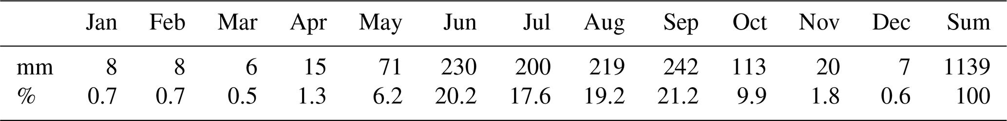
^* Hydro-Administrative Region V includes the basin of the state of Oaxaca and part of the state of Guerrero flowing to the Pacific. Source: CONAGUA (2016).

Table B2 Confusion matrix of land cover classification.

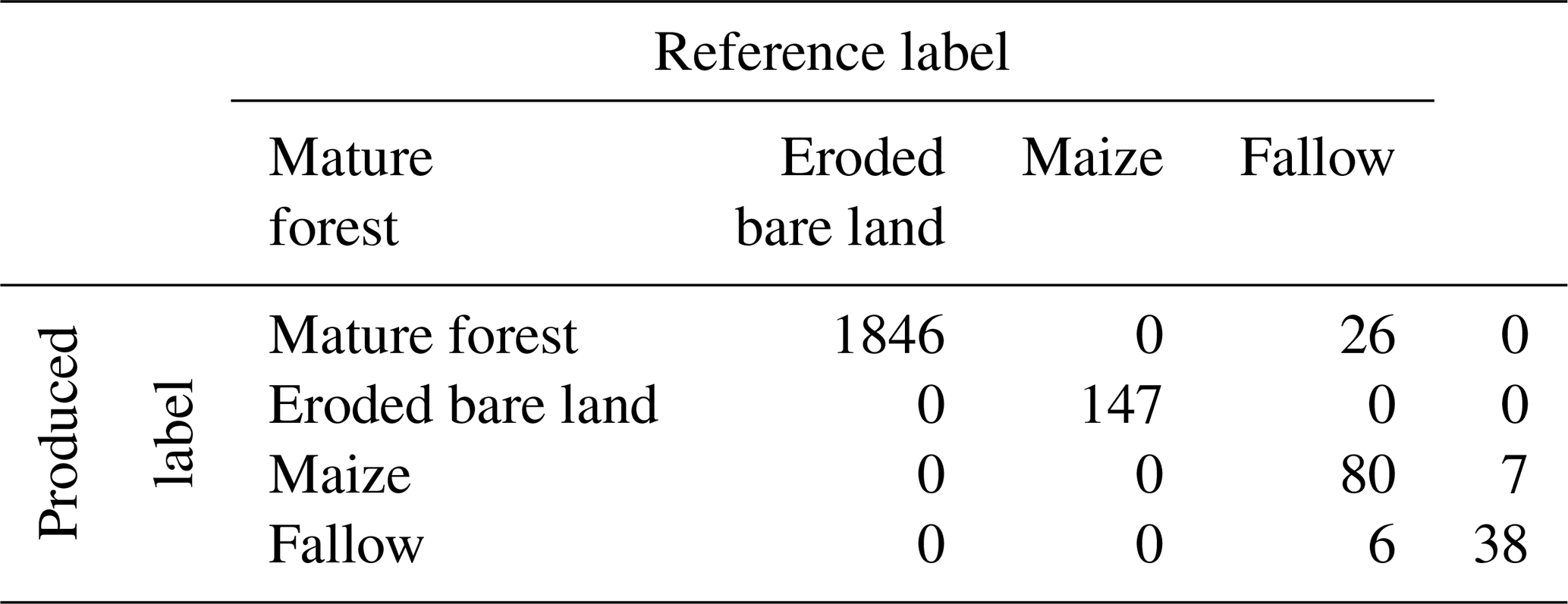
Table B3 Land-cover-based OpenLISEM parameterization for the Cuauhtemoc watershed.

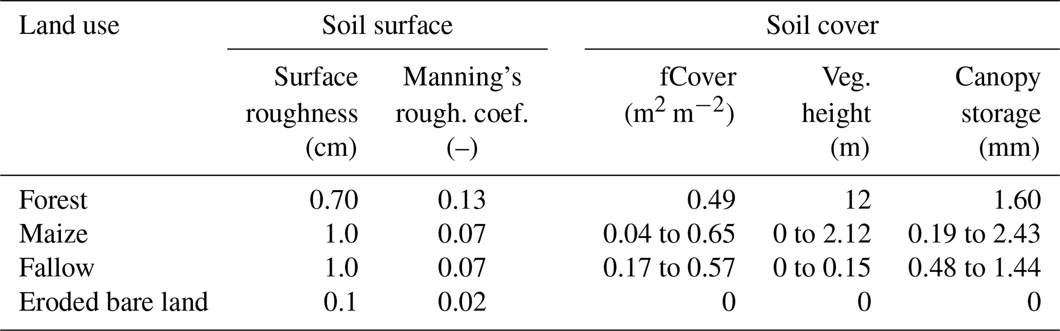
Table B4 Soil-type-based OpenLISEM parameterization for the Cuauhtemoc watershed.

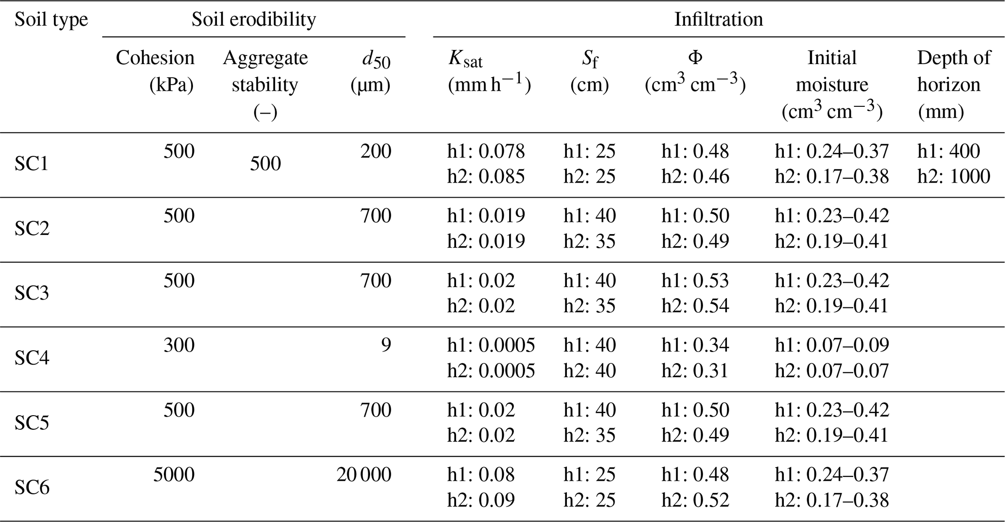
Table B5 Channel OpenLISEM parameterization for the Cuauhtemoc watershed.

Table B6 Collected sediment at study units.

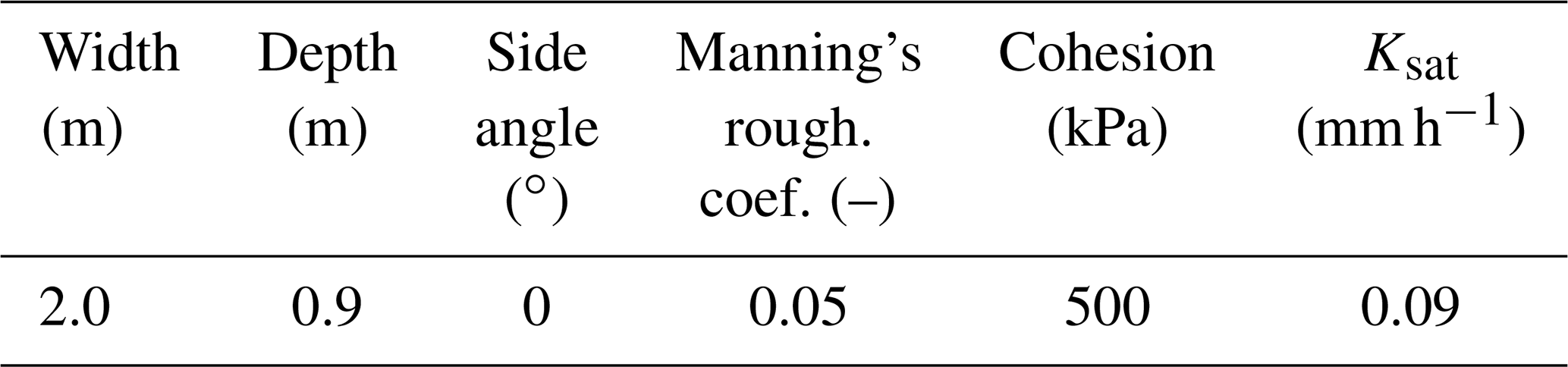
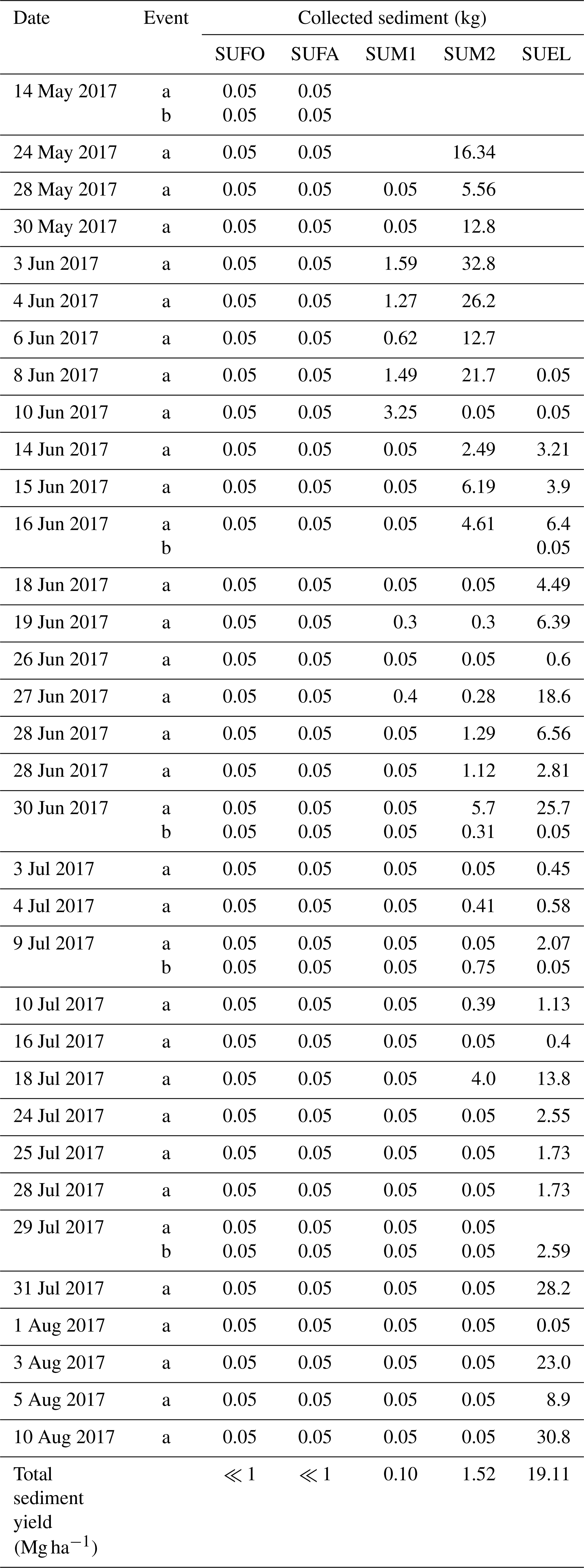
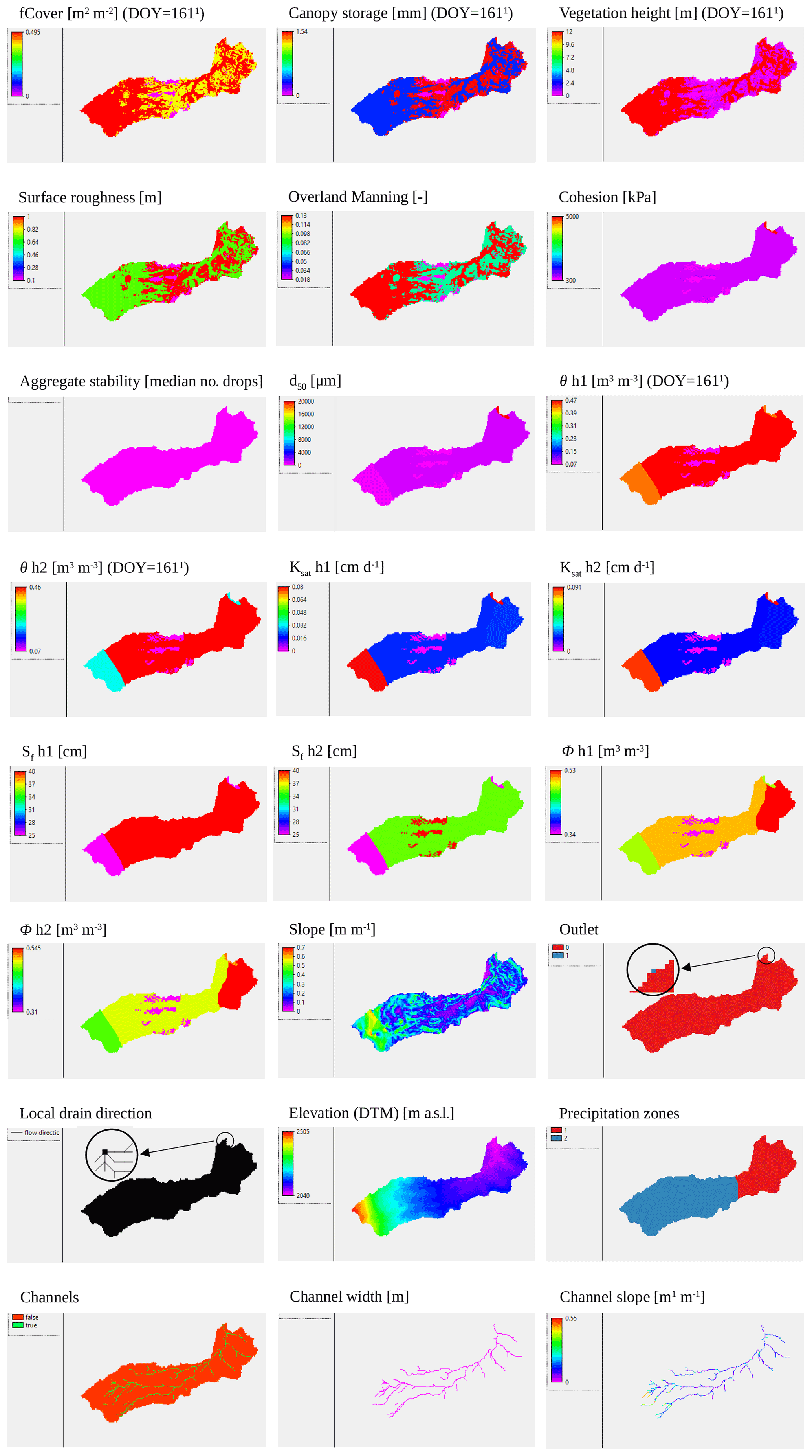
Figure B1 Maps of input parameters. ¹ Day of the year (DOY) 161 corresponds to 10 June 2017 and 34 d after maize in SUM was planted. Notes: values of the aggregate stability map are as per Table B4. Maps of horizon depth 1 and 2 are constant (similar to aggregate stability map), as per Table B4. Values of channel depth, side angle, Manning's roughness, cohesion, and K_sat are constant (similar to channel width), as per Table B5.

Figure B2 Cumulative soil loss (Mg ha⁻¹) per land cover across resolutions.