Advanced sensitivity analysis of the impact of the temporal distribution and intensity of rainfall on hydrograph parameters in urban catchments

Knowledge of the variability of the hydrograph of outflow from urban catchments is highly important for measurements and evaluation of the operation of sewer networks. Currently, hydrodynamic models are most frequently used for hydrograph modeling. Since a large number of their parameters have to be identified, there may be problems at the calibration stage. Hence, sensitivity analysis is used to limit the number of parameters. However, the current sensitivity analytical methods ignore the effect of the temporal distribution and intensity of precipitation in a rainfall event on the catchment outflow hydrograph. This article presents a methodology of constructing a simulator of catchment outflow hydrograph parameters (volume and maximum flow). For this purpose, uncertainty analytical results obtained with the use of the GLUE (generalized likelihood uncertainty estimation) method were used. A novel analysis of the sensitivity of the hydrodynamic catchment models was also developed, which can be used in the analysis of the operation of stormwater networks and underground infrastructure facilities. Using the logistic regression method, an innovative sensitivity coefficient was proposed to study the impact of the variability of the parameters of the hydrodynamic model depending on the distribution of rainfall, the origin of rainfall (on the Chomicz scale), and the uncertainty of the estimated simulator coefficients on the parameters of the outflow hydrograph. The developed model enables the analysis of the impact of the identified SWMM (Storm Water Management Model) parameters on the runoff hydrograph, taking into account local rainfall conditions, which have not been analyzed thus far. Compared with the currently developed methods, the analyses included the impact of the uncertainty of the identified coefficients in the logistic regression model on the results of the sensitivity coefficient calculation. This aspect has not been taken into account in the sensitivity analytical methods thus far, although this approach evaluates the reliability of the simulation results. The results indicated a considerable influence of rainfall distribution and intensity on the sensitivity factors. The greater the intensity and rainfall were, the lower the impact of the identified hydrodynamic model parameters on the hydrograph parameters. Additionally, the calculations confirmed the significant impact of the uncertainty of the estimated coefficient in the simulator on the sensitivity coefficients. In the context of the sensitivity analysis, the obtained results have a significant effect on the interpretation of the relationships obtained. The approach presented in this study can be widely applied at the model calibration stage and for appropriate selection of hydrographs for identification and validation of model parameters. The results of the calculations obtained in this study indicate the suitability of including the origin of rainfall in the sensitivity analysis and calibration of hydrodynamic models, which results from the different sensitivities of models for normal, heavy, and torrential rain types. In this context, it is necessary to first divide the rainfall data by origin, for which analyses will be performed, including sensitivity analysis and calibration. Considering the obtained results of the calculations, at the stage of identifying the parameters of hydrodynamic models and their validation, precipitation conditions should be included because, for the precipitation caused by heavy rainfall, the values of the sensitivity coefficients were much lower than for torrential ones. Taking into account the values of the sensitivity coefficients obtained, the calibration of the models should not only cover episodes with high rainfall intensity, since this may lead to calculation errors at the stage of applying the model in practice (assessment of the stormwater system operating conditions, design of reservoirs and flow control devices, green infrastructure, etc.).

1 Introduction

Climate change and progressive urbanization result in an increase in the volume of stormwater outflow from catchments, which leads to flooding and deterioration of water quality in receivers (Crocetti et al., 2020; Fletcher et al., 2013). To reduce the incidence of these phenomena, runoff model generation is needed. This can be achieved using hydrodynamic models based on physical equations representing stormwater outflows. One of the common tools is the SWMM (Storm Water Management Model) program (Buahin and Horsburgh, 2015; Crocetti et al., 2020; Gironás et al., 2010). SWMM allows for simulation of sewage quantity (Guan et al., 2015), quality (Dotto et al., 2012), including objects located in sewer networks (separation and combined sewer networks. The program allows for simulation of surface runoff from a drainage basin including the flow in a network of pipes and analysis of interaction between hydraulic conditions in the system and sewage flooding on the ground (Fraga et al., 2016). The program's advantages also include the possibility to model green infrastructure facilities (McGarity et al., 2013). The source code of the program is available to users, which gives the possibility of its modification and adaptation to individual requirements. Due to the interactions between parameters identified in the models, they may be difficult to calibrate, and the results may be biased. Therefore, statistical models are used for the simulation of runoff, which has been shown in a number of studies (Gernaey et al., 2011; Yang and Chui, 2020). A serious drawback of many models (the so-called black-box techniques) is their inability to interpret structural parameters (Zoppou, 2001). Linear models, including multiple linear regression (MLR), as well as nonlinear models such as artificial neural networks (ANNs) and classification and regression trees (CRTs) with their modifications (Yang and Chui, 2020), are used for this purpose. Nonlinear models enable a more accurate description of hydrological processes in urban catchments, which results from the physics of the analyzed phenomena and is confirmed in the literature (Zoppou, 2001).

The hydrodynamic model must be calibrated to reflect the conditions prevailing in the real system. Calibration of the catchment model is a complex task aimed at determining the optimal values of parameters with a satisfactory goodness of fit of calculation outcomes and measurement results (Bárdossy, 2007; Dotto et al., 2012; Guan et al., 2015). Parameter values are determined for an appropriate form of the objective function in which one or more criteria (maximum instantaneous flow, hydrograph volume, or mean relative or absolute error of flow prediction) can be included. Since the description of the stormwater outflow from the catchment is complicated, modeling the phenomenon requires knowledge of many parameters (physical and geographic characteristics of the catchment and sewer network). A number of these parameters can be determined using detailed spatial data (GIS, geographic information system), as has been indicated in numerous studies (Fraga et al., 2016; Leandro and Martins, 2016). This helps to reduce the number of variables included in the calibration. However, since a large number of parameters must be included in the models, there may be problems with the identification of their values. Therefore, the aim is usually to simplify the calibration process by eliminating factors that have a negligible impact on simulation results. Hence, model sensitivity analysis is employed. To understand the modeled processes in urban catchments and to determine the influence of interactions between the identified parameters on the simulation results, an uncertainty analysis (GLUE – generalized likelihood uncertainty estimation) is performed. This method is widely used in the analysis of the quantity and quality of stormwater for models of urban and agricultural catchments (Dotto et al., 2012; Mirzaei et al., 2015), retention reservoirs (Kiczko et al., 2018), stormwater flooding (Fraga et al., 2016), etc., which is reflected in a large number of publications in this field. In this approach, the empirical distributions of parameters identified in hydrodynamic models are determined (catchment retention, roughness coefficients of pervious and impervious areas, roughness of channels, etc.) and a confidence interval is determined (e.g., 95 %), containing the data obtained from the measurement results.

As shown by the literature (Chisari et al., 2018; Tolley et al., 2019; Xu et al., 2019), the analysis is often applied at the stage of calibration of the mathematical models. In practice, local and global sensitivity analytical methods, which can be implemented for statistical and physical relationships, are used (Link et al., 2018; Morio, 2011; Cristiano et al., 2019). In the case of the local sensitivity analysis, the calculations consist of determination of the derivative value at a given point, which is the basis for assessment of the effect of the variance of the variables on the modeled value (Razavi and Gupta, 2015). One of the drawbacks of the local sensitivity analysis is the fact that the variability of the analyzed phenomenon and the effect of variables are considered in the narrow domain of the modeled variable (Pianosi et al., 2016). This approach ignores the fact that the sensitivity of the model in the domain of the output values may change, which may be important for calibration of the model at the validation stage and its course. In the case of nonlinear models, the local sensitivity analysis does not take into account the character of the relationships between the explanatory variables and dependent variable. Then, the sensitivity coefficient is calculated only for the mean level of the explanatory variable. Nevertheless, this method is widely used in the analysis of the sensitivity of models describing runoff in urban catchments, which has been confirmed by numerous studies (Ballinas-González et al., 2020; Liu et al., 2020; Yang et al., 2019). Another shortcoming of sensitivity analysis based on partial derivatives is the fact that the effects of individual variables on the output variable are estimated while the other variables are kept constant. This is rarely observed in the case of complex relationships, as the explanatory variables are then correlated to some extent. The ceteris paribus analysis does not take this fact into account. Consequently, the effects of individual variables may be overestimated.

In the context of literature studies (Xu et al., 2019), the results of LSAs (local sensitivity analyses) may lead to simplifications in the interpretation of hydrological processes in catchments. From the point of view of the appropriate selection of the identified parameters of urban catchment models, the local sensitivity analytical method has limited application and may lead to problems with calibration (Morio, 2011). Global sensitivity analysis does not have many of the aforementioned disadvantages. One of the simplest methods used in many cases is based on multiple linear regression (Ashley and Parmeter, 2020; Touil et al., 2016). However, the results of the sensitivity analysis can be considered reliable when the coefficient of determination reflecting the relationship between the dependent variable and explanatory variables is not lower than 0.70. When this requirement is not met, other methods for global sensitivity analysis should be applied (Saltelli et al., 2007). Variance methods, which facilitate estimation of the contribution of the individual parameters to the model output variance using the Monte Carlo method, are more precise and more computationally complex. The global sensitivity analysis (GSA) method is one of the commonly used approaches. It has been subjected to modifications, as described in Iooss and Lemaître (2015). Variance methods are currently gaining increasing interest, which is confirmed by the number of publications in this field. However, since implementation is complicated, simplified methods are used in many cases despite the major advantage of variance approaches over local analytical methods. The implementation of global sensitivity analytical methods is not a simple task, as it requires complex mathematical tools, which limits their application. Despite the limitations of the local sensitivity analytical method and the complex implementation of the global sensitivity analysis, in both cases, the aspects related to local precipitation conditions are treated to a limited extent. Recent studies of urban catchments indicate that the temporal and spatial distributions of rainfall are very important factors that strongly influence the catchment response (Schilling, 1991; Berne et al., 2004; Ochoa-Rodriguez et al., 2015; Cristiano et al., 2017). However, a number of issues have not been fully clarified. In the currently used methods, the influence of rainfall origin on the results of the sensitivity analysis is neglected. It is not clear how the sensitivity of the model (maximum flow rate and hydrograph volume) changes for rainfall events resulting from high (convective) or low intensity (convergence zone) rainfall. The LSA and GSA methods ignore the influence of rainfall temporal distribution on the sensitivity coefficients, which is contrary to the information from the literature (Schilling et al., 1991) describing the analyses conducted for different urban catchments. It is important to select outflow hydrographs from the catchment area for the identification of parameters and their validation in the context of rainfall parameters (rainfall origin, rainfall intensity, and temporal distribution). It is also of great methodological importance in the context of modifying the currently used methods of sensitivity analysis of hydrodynamic catchment models. In the sensitivity analytical methods based on statistical models, the influence of the uncertainty of the estimated coefficients on the sensitivity coefficients is neglected. From the point of view of the reliability of the obtained results, this is important when deciding on the selection of the method of parameter identification in hydrodynamic models (GIS, maps, etc.) to reduce the uncertainty of the simulation results.

Given the information specified above, this paper presents an original application of the logistic regression method for sensitivity analysis. This is one of the first studies to analyze the sensitivity of the model in terms of the temporal variability of rainfall. The advantage of the model is the fact that it has the form of a statistical relationship; hence, without the need for complex analyses, it can be used to determine the effects of parameters included in the calibration of the catchment model, precipitation characteristics, and absolute values of the modeled dependent variables on the parameters of outflow hydrographs (maximum instantaneous flow and hydrograph volume). The approach proposed in the present study also facilitates analysis of the sensitivity of selected explanatory variables, depending on the numerical values of the modeled hydrograph parameters of catchment runoff. At the stage of sensitivity analysis, the effect of the uncertainty of coefficients estimated in the statistical model (logistic regression) on the calculated results is included, which is reflected in the determined sensitivity coefficients. Since the model is constructed based on simulation results provided by the Monte Carlo method, which is typical for global sensitivity analytical methods, this approach can complement and extend the results of GSA calculations. In summary, (Saltelli et al., 2007; Razavi and Gupta, 2015), the sensitivity analysis used in the present study represents a fusion of local and global sensitivity analysis through a combination of logistic regression in phenomenon modeling with partial derivatives. Since logistic regression is not an example of a black-box method, as it has an explicit form of dependence between the modeled probability of success and explanatory variables, the use of partial derivatives for assessment of the sensitivity of the model to individual parameters seems reasonable. Especially in the case of an implicit, complex, and nonlinear dependence, it is recommended that variance-based techniques such as the Sobol method be employed. Partial derivatives used in the logistic regression model increase the flexibility of this method, as it is possible to assess the model sensitivity to individual parameters at any point in the domain. An additional modification can be the use of a standardized local sensitivity analytical method based on logarithms of dependent and explanatory variables. This facilitates assessment of the effect of the percentage increase in the explanatory variable on the percentage increase in the dependent variable.

Due to the extensive nature of the conducted analyses, the article has been divided into several sections, including characteristics of the research object and methodology, which presents an innovative algorithm for the development of a logistic regression model and subsequent calculation steps, i.e., determination of a hydrodynamic model of a catchment, identification of the threshold values of the outflow hydrograph parameters from a catchment using a hydrodynamic model, uncertainty analysis using the GLUE method, development of a logit model and its verification, analysis of the influence of rainfall origin and temporal distribution of rainfall on the calculated sensitivity coefficients, and assessment of the impact of uncertainty of the identified coefficients in the logit model on the values of the sensitivity coefficients.

Figure 1 Scheme of the hydrodynamic model of the catchment generated in the SWMM program.

2 Case study

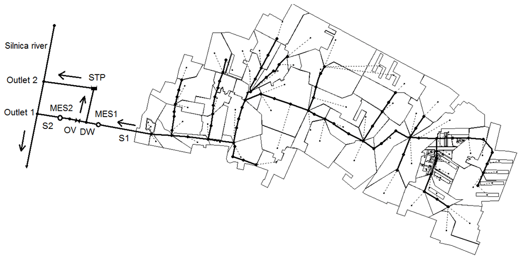
The analysis in this study was carried out in a catchment with a total area of 62 ha located in the southeastern part of the city of Kielce, central Poland (Fig. 1). Six types of impervious surfaces were distinguished in the catchment: sidewalks, roads, parking lots, greenery, school playgrounds, and roofs (with 72.5 % of their area directly connected to the stormwater sewer system). The main canal is 1.6 km long with a diameter in the range of ∅ 0.60–1.25 m. Detailed information concerning the analyzed catchment was provided by Kiczko et al. (2018). The analysis of measurement data (2010–2016) from the catchment distinguished a dry period of 0.16–60 d. The annual precipitation depth was 537–757 mm, and the number of days with precipitation was in the range of 155–266. The number of storms per year in the analyzed period ranged from 27 to 47. The area was characterized by an average annual temperature of 8.1–9.6 ^∘C and 36–84 snowfall days. The analysis of flow measurement data recorded with a MES1 flow meter revealed that the instantaneous stormwater stream in the dry periods was in the range of 0.001–0.009 m³ s⁻¹, which indicates an infiltration effect in the sewer network.

The analyzed sewer system consists of 200 manholes and 100 conduit sections with ∅ 0.20–1.25 m diameters and longitudinal slopes of 0.1 %–2.7 %, which gives a retention capacity of 2032 m³. Manning's roughness coefficient for the conduit is in the range of 0.010–0.018 ${\mathrm{m}}^{-\mathrm{1}/\mathrm{3}}\mathrm{s}$. The average retention depth is 2.5 mm in the impervious areas and 6.0 mm in the pervious surfaces, which gives a weighted mean of 3.81 mm for the entire catchment. Stormwater is discharged from the catchment through the S1 channel to the diversion chamber (DC), and some part is discharged directly to the stormwater treatment plant (STP) to a filling level of h_m = 0.42 m. After exceeding the h_m value, the stormwater is discharged via the stormwater overflow (OV) into channel S2, which discharges the stormwater into the Silnica river.

As part of the continuous monitoring carried out in 2009–2011, the volume of stormwater outflow from the catchment was measured using a flow meter installed in the S1 channel at a distance of 3.0 m from the inlet to the diversion chamber (DW). In turn, in 2015, parallel MES1 and MES2 flow meters were installed in the inlet (S1) and discharge (S2) channels to measure the flow and stormwater level. A detailed description of the stormwater catchment and installed measuring equipment is provided in Szeląg (2016).

The catchment (Fig. 1) had previously been analyzed to determine the variability of the quantity and quality of stormwater and the operation of the sewer system based on the catchment hydrodynamic model generated in the SWMM program. The model used in the study was subjected to deterministic (Szelag et al., 2016) and probabilistic (Kiczko et al., 2018) calibration and was used as the basis for the sensitivity analysis. It was also subjected to probabilistic calibration with the GLUE+GSA method (Szelag et al., 2016). The deterministic calibration was perceived in the present study as a computational case where the uncertainty and interaction of calibrated parameters in the SWMM were omitted. The parameters were determined with the method of successive substitutions to achieve a sufficiently high degree of agreement between the modeled and measured hydrographs.

3 Methodology

The developed methodology of the sensitivity analysis of hydrodynamic models included several independent stages: preparation of data for the construction of the model and its implementation, conducting the uncertainty analysis using the GLUE method, development of a logit model for specific threshold values of the hydrograph parameters and model verification, and calculation of sensitivity coefficients, taking into account the rainfall origin, the temporal distribution of rainfall, and the evaluation of the impact of the uncertainty of the identified coefficients in the logit model on the results of the sensitivity analysis.

3.1 Rainfall and separation of independent rainfall events

The methodology described in the DWA-A 118E (2006) guidelines was applied in the study to separate independent rainfall events. The interval between successive independent rainfall events was 4 h (Dunkerley, 2008; Joo et al., 2014; Szeląg et al., 2021). The minimum rainfall depth (3.0 mm) constituting a rainfall event was adopted, as in the studies conducted by Fu et al. (2011) and Fu and Butler (2014).

Figure 2 Calculation algorithm scheme in a logit model.

3.2 Scheme of model analysis

In the present study, a method of model sensitivity analysis was proposed to predict the stormwater volume (maximum instantaneous flow and hydrograph volume) with the use of logistic regression (Fig. 2). The method presented here represents a group of sensitivity analytical methods based on empirical models. It was assumed that the variable rainfall distribution may exert different effects on the sensitivity of the model and induce changes in the calibrated parameters. It was also assumed that the sensitivity of the model may change as a result of an increase in the maximum instantaneous stormwater flow and the volume of the outflow hydrograph. Due to the nonlinearity between the modeled hydrograph parameters and the calibrated model coefficients, use of the linear approach is limited (Chan et al., 2018); therefore, the classification model (logit) was used in the study. Appropriate threshold values of hydrograph parameters constituting the basis for substitution of continuous values with classes were selected in the model.

On the one hand, this approach is based on the precipitation dynamics during rainfall events specified in the DWA-A 118E (2006) guidelines (distribution R1 – constant rainfall intensity during a rainfall event; distribution R2 – maximum rainfall intensity in the middle of the rainfall event, i.e., $t/t_{\mathrm{r}}$ = 0.50; distribution R3 – maximum rainfall intensity, i.e., for $t/t_{\mathrm{r}}$ = 0.85–1.00; and distribution R4 – maximum rainfall intensity in the initial phase of rainfall). The approach assumed in this paper was confirmed by the analyses of numerous researchers conducting computer simulations of the operation of the stormwater network for various rainfall parameters, including the analysis of the conditions of the total system functioning (Siekmann and Pinnekamp, 2011), the location of green infrastructure objects (Jia et al., 2015), and the location of underground infrastructure facilities allowing real-time control of the flow in channels or at the outflow from reservoirs (Garofalo et al., 2017).

Table 1 Ranges of SWMM coefficients (Kiczko et al., 2018).

On the other hand, the modeled hydrograph parameter values were combined with the rainfall classification, which facilitated generalization of the analytical results. Compared with the local and global analytical methods, detailed analysis of changes in the sensitivity to the effect of calibrated coefficients was possible with the proposed approach, taking into account values of the modeled parameters of the catchment outflow hydrograph. This has been scarcely considered in this approach thus far. The calculation algorithm presented in this study consists of three elements (Fig. 2). The first comprises a simulator of parameters of the catchment outflow hydrograph (statistical model generated with the logistic regression method), which includes rainfall characteristics and coefficients calibrated in the hydrodynamic catchment model. The simulator was constructed based on simulations performed with the use of calculations in the catchment model, which included the uncertainty of the identified coefficients subjected to calibration. The approach proposed here is applied in computational experiments at the stage of generation of mathematical models for urban catchments, as described by Thorndahl et al. (2009). It is important that the distribution of coefficients (Table 1) used for GLM (generalized likelihood model) identification should result from their actual variability. The distribution can be determined by probabilistic identification of calibrated coefficients. The GLUE methodology, in which the variability of calibrated coefficients is determined by selecting the so-called behavioral simulations, was employed in this study. Based on a posteriori distributions of calibrated coefficients in the catchment model determined by observation data, simulations of catchment outflow hydrographs were performed based on the separated rainfall events in continuous rainfall time series (2010–2016), for which typical temporal rainfall distribution was assumed independently (R1, R2, R3, and R4). This was the basis for determination of the outflow hydrograph parameters – maximum instantaneous flow (Q_m) and hydrograph volume (V).

The second stage consisted of establishing the so-called threshold values of maximum flow (Q_m,g) and hydrograph volume (V_g), which served as the basis for the division into rainfall events with different intensities and their temporal distribution in the time series (ξ = R1, R2, R3, and R4). Establishment of general rules for selection of threshold values may be very difficult, as they are the result of the response of the catchment to rainfall, which is catchment-specific. These may be characteristic values of flows influenced by the presence of objects in the sewer network (e.g., stormwater overflows) at which they begin to operate. An alternative approach is to apply rainfall classification measures (proposed by Chomicz, 1951; Sumner, 1988; etc.), which allow for determination of the characteristic parameters of hydrographs. Sumner's classification is universal in its nature and – like the Chomicz classification – it expresses the qualitative relationship between the category of rainfall and its intensity. Hence, belonging to the appropriate rainfall class can be associated with the average rainfall intensity. The rainfall classes on the Sumner scale determine the extremely different hydraulic conditions prevailing in the stormwater network, which may not always be used in practice for measurements and calibration. In the case of the Chomicz classification, a number of rainfall categories were introduced, ranging from normal to heavy rain and ending with torrential rain. This approach makes it possible to identify the operating conditions of the stormwater network and facilities located in it, taking into account the rainfall data, i.e., rainfall duration (t_r) and rainfall depth (P_tot) within the appropriate range of variability. This is important because it enables the identification of the average intensity of rainfall (i = $P_{\text{tot}}\cdot t_{\mathrm{r}}^{-\mathrm{1}}$) as a parameter connected with the operation of the stormwater system, which can be associated with runoff from the catchment and hydrograph parameters (volume and maximal flow rate).

In the present study, the reference rainfall values determined at the regional classification scale proposed by Chomicz (1951) were the basis for the selection of threshold values (maximum instantaneous flow and hydrograph volume) in accordance with the following equation:

$$\begin{array}{}\text{(1)}& P_{\text{tot}}=U={\mathit{\alpha }}_{\mathrm{0}}\cdot \sqrt{t_{\mathrm{r}}},\end{array}$$

where t_r is the rainfall duration, P_tot is the rainfall depth equal to its efficiency, and α₀ is the rainfall efficiency coefficient taking into account the normal, heavy, and torrential rain types.

Based on the Chomicz (1951) classification of rainfall, outflow hydrographs were calculated, their parameters (Q_m and V) were determined, and classification variables were defined. The outflow hydrographs and their parameters (volume and maximum flow rate) were calculated for the set values P_tot = f(t_r, α₀), which matched the assumed categories of rainfall and the temporal distribution of rainfall in the rainfall episode. When the calculated values Q(P_tot, t_r, ζ, θ) and V(P_tot, t_r, ζ, θ) (where ζ is a function describing the temporal intensity distribution, and θ is a function taking into account the uncertainty of the calibrated parameters in the catchment model) are smaller than the threshold values, they have a value of 0; otherwise, they are equal to 1.

In the third stage, logistic regression models were developed for the values of the explanatory variables (P_tot, t_r, ζ, and x_j – values of calibrated coefficients in the catchment model; rainfall characteristics) and for the established dependent (zero-one) variables for the applied threshold values (Q_g,m and V_g) and temporal rainfall distribution (ζ). The subsequent stage of the analyses consisted of determination of the values of the sensitivity coefficients (S_xj) in accordance with the methodology described later in this study. The proposed computational algorithm of the sensitivity analysis was performed in the following stages:

• a.

  Determination of the hydrodynamic model of the catchment;

• b.

  Identification of a posteriori distributions of the calibrated parameters in the model of the catchment;

• c.

  Monte Carlo sampling of the identified parameters of the SWMM and calculation of the parameters of the outflow hydrograph from the catchment for the separated rainfall events (described by the temporal distribution of rainfall and duration of rainfall, as well as rainfall depth);

• d.

  Identification of the threshold values of the outflow hydrograph parameters from the catchment, taking into account the origin of rainfall (on the Chomicz scale);

• e.

  Determination of logit models and their validation using a hydrodynamic model;

• f.

  Calculation of sensitivity coefficients, taking into account the origins of rainfall and the temporal distribution of rainfall;

• g.

  Determination of the influence of uncertainty of estimated coefficients in logistic regression models on the sensitivity coefficients.

Based on the calculation scheme described above, this paper presents the next stages of construction of a logit model. A catchment model generated in the SWMM program was used for this purpose. The threshold values were determined in accordance with the Chomicz (1951) classification, in which the following categories of rainfall were defined: normal rain (α₀ = 1.00), heavy rain (α₀ = 1.40), and torrential rain (α₀ = 5.66), assuming a constant temporal rainfall distribution and rainfall duration of t_r = 15 min. For these assumptions, the depth of rainfall was determined from Eq. (1), and catchment outflow hydrographs were simulated using the calibrated catchment model.

3.3 Logistic regression

The logistic regression model, also known as the binomial logit model, is usually employed for the analysis of binary data and can be used to determine the probability and identify the occurrence of events (Jato-Espino et al., 2018; Li and Willems, 2019; Szeląg et al., 2020). The maximum amount of stormwater outflow from the catchment and the hydrograph parameters of any rainfall event can be calculated using hydrodynamic models, e.g., SWMM. An alternative solution is statistical models (hydrograph simulators are considerably easier to implement than physical models); for instance, the generalized linear model (GLM – generalized likelihood model), which comprises the variability of rainfall characteristics and the uncertainty of calibrated coefficients, is shown in the following equation:

$$\begin{array}{}\text{(2)}& \begin{array}{rl}Q(\mathit{\mu }{)}_{\mathrm{m}}& ={\mathit{\alpha }}_{\mathrm{0}}+{\mathit{\alpha }}_{\mathrm{1}}\cdot P_{\mathrm{c}}+{\mathit{\alpha }}_{\mathrm{2}}\cdot t_{\mathrm{d}}+{\mathit{\alpha }}_{\mathrm{3}}\cdot x_{\mathrm{1}}+{\mathit{\alpha }}_{\mathrm{4}}\cdot x_{\mathrm{2}}+\mathrm{\cdots }\\ & +{\mathit{\alpha }}_{\mathrm{j}+\mathrm{2}}\cdot x_{\mathrm{j}},\end{array}\end{array}$$

where α₀ represents intercept; α₁, α₂, …, α_j+2 represent empirical coefficients determined with the maximum likelihood method; P_tot represents rainfall depth; t_r represents rainfall duration; $x_{\mathrm{1},\mathrm{2},j=n}$ represents calibrated coefficients in the SWMM; and Q_m represents the link function determining the relationship of the mean value of the dependent variable μ with the linear combination of predictors.

Assuming that μ = p and introducing the link function referred to as logit, it is possible to transform the modeled values of dependent variables included in Eq. (2) into a new (zero-one) system describing the probability values:

$$\begin{array}{}\text{(3)}& \begin{array}{rl}Q\left(p\right)=Q(\mathit{\mu }{)}_{\mathrm{m}}=& \text{logit}\left(p\right)=\ln \left({\displaystyle \frac{p}{\mathrm{1}-p}}\right)\\ =& \exp ({\mathit{\alpha }}_{\mathrm{0}}+{\mathit{\alpha }}_{\mathrm{1}}\cdot P_{\text{tot}}+{\mathit{\alpha }}_{\mathrm{2}}\cdot t_{\mathrm{r}}+{\mathit{\alpha }}_{\mathrm{3}}\cdot x_{\mathrm{1}}\\ & +{\mathit{\alpha }}_{\mathrm{4}}\cdot x_{\mathrm{2}}+\mathrm{\cdots }+{\mathit{\alpha }}_{\mathrm{j}+\mathrm{2}}\cdot x_{\mathrm{j}}).\end{array}\end{array}$$

This approach may prove especially useful when the results of calculations in the multiple linear regression model exhibit unsatisfactory convergence (R² < 0.70), and it is therefore advisable to introduce classification variables, which is a simplifying solution. Moreover, this approach makes it possible to emphasize and include relationships that might be omitted in the calculations of multiple linear regression, as has been demonstrated in many reports (Hosmer and Lemeshow, 2000; Kleinbaum and Klein, 2010; Myers et al., 2010). Since the continuous values Q(P_tot, t_r, x_j)_m are transformed into the probability space p by the logit function in this case, it is reasonable to equate them with the determined p(P_tot, t_r, x_j) values for a given threshold Q_g,m (Fig. 2). In the transformed data system (expressing probability) varying in the range of 0–1, it was shown that the effect of the change in individual variables (x_j) by Δx_j on the p value is described by the following equation:

$$\begin{array}{}\text{(4)}& \begin{array}{rl}{S}_{x_{\mathrm{j}}}=& {\displaystyle \frac{\partial p}{\partial x_{\mathrm{j}}}}\cdot {\displaystyle \frac{x_{\mathrm{j}}}{p}}={\displaystyle \frac{p(x_{\mathrm{j},\mathrm{g}}+\mathrm{\Delta }{x}_{\mathrm{j}})-p(x_{\mathrm{j},\mathrm{g}};Q_{\mathrm{g},\mathrm{m}})}{(x_{\mathrm{j},\mathrm{g}}+\mathrm{\Delta }{x}_{\mathrm{j}})-x_{\mathrm{g},\mathrm{j}}}}\\ & \cdot {\displaystyle \frac{x_{\mathrm{j}}}{p(x_{\mathrm{j},\mathrm{g}};Q_{\mathrm{g},\mathrm{m}})}}\\ =& {\mathit{\alpha }}_{\mathrm{j}+\mathrm{2}}\cdot x_{\mathrm{j}}\cdot (\mathrm{1}-p(x_{\mathrm{j},\mathrm{g}};Q_{\mathrm{g},\mathrm{m}}\left)\right),\end{array}\end{array}$$

where Q and $p(x_{\mathrm{j},\mathrm{g}}+\mathrm{\Delta }{x}_{\mathrm{j}})$ represent maximum flow value (Fig. 2a) and the probability of exceeding thereof for value ($x_{\mathrm{j},\mathrm{g}}+\mathrm{\Delta }{x}_{\mathrm{j}})$, respectively (Fig. 2b); $Q(x_{\mathrm{j},\mathrm{g}}{)}_{\mathrm{m},\mathrm{g}}$ represents maximum instantaneous outflow from the catchment; and $p(x_{\mathrm{j},\mathrm{g}};Q_{\mathrm{m},\mathrm{g}})$ represents probability of exceeding the threshold value Q_g,m for the given explanatory variables (P_tot, t_r, x₁, x₂, x₃, …, x_n) equal to p = 0.50 (most considerations in the present analyses related to the value p = 0.50, as this value corresponds to that of Q_g,m in the probability scale p).

Figure 3 Calculation diagram showing the effect of changes in the x_j,g value by Δx_j on (a) the flow volume Q_m and (b) probability of exceeding p(Q_g,m; x_j,g) = 0.50.

As indicated in Fig. 3, an increase in x_j,g by Δx_j results in a decrease in the Q_g,m value by ΔQ_m and yields a flow value of Q_ξ, which facilitates determination of the numerical value of the sensitivity coefficient described by Eq. (4). In the transformed space (see Fig. 2b), the increase in the x_j,g value (corresponding to p = 0.50 and the threshold value Q_g,m) to the value of $x_{\mathrm{j},\mathrm{g}}+\mathrm{\Delta }{x}_{\mathrm{j}}$ is accompanied by a decline in the p value by Δp to the value p^∗. In these analyses, the determined p^∗ value corresponds to $Q_{\mathrm{m}}^{\ast }$, which can be defined as Q_g,m – $f(p,p^{\ast })$, and the relationship can be expressed as follows:

$$\begin{array}{}\text{(5)}& \begin{array}{rl}{S}_{x_{\mathrm{j}}}& ={\displaystyle \frac{Q(x_{\mathrm{j},\mathrm{g}}+\mathit{\epsilon }\cdot \mathrm{\Delta }{x}_{\mathrm{j}}{)}_{\mathrm{m}}^{\ast }-Q(x_{\mathrm{j},\mathrm{g}}{)}_{\mathrm{g},\mathrm{m}}}{(x_{\mathrm{j},\mathrm{g}}+\mathit{\epsilon }\cdot \mathrm{\Delta }{x}_{\mathrm{j}})-x_{\mathrm{j},\mathrm{g}}}}\cdot {\displaystyle \frac{x_{\mathrm{j}}}{Q(x_{\mathrm{j},\mathrm{g}}{)}_{\mathrm{g},\mathrm{m}}}}\\ & ={\displaystyle \frac{f(p,p^{\ast })-Q(x_{\mathrm{j},\mathrm{g}}{)}_{\mathrm{g},\mathrm{m}}}{(x_{\mathrm{j},\mathrm{g}}+\mathit{\epsilon }\cdot \mathrm{\Delta }{x}_{\mathrm{j}})-x_{\mathrm{j},\mathrm{g}}}}\cdot {\displaystyle \frac{x_{\mathrm{j}}}{Q(x_{\mathrm{j},\mathrm{g}}{)}_{\mathrm{g},\mathrm{m}}}},\end{array}\end{array}$$

where ε is the empirical coefficient for conversion of the $Q_{\mathrm{m}}^{\ast }$ value into p^∗. The p^∗ value can be related to $Q_{\mathrm{m}}^{\ast }$ < Q_m,g; hence, the effect of changes in the x_j value on the calculated results can be inferred, and the sensitivity coefficient can be determined from Eq. (5). Assuming a p value of 0.50 for the analyses was driven by the fact that the logit models determined should be universal, which is important from the point of view of being able to generalize the results obtained and apply them also to other urban catchments (Jato-Espino et al., 2018; Li and Willems, 2019; Szeląg et al., 2020).

The following parameters were included in the assessment of the predictive abilities of logit models: sensitivity – SENS (reflects the correctness of classification of data in a dataset p > p(Q_g,m)), specificity – SPEC (reflects the correctness of classification of data in a dataset p < p(Q_g,m)), and calculation error – $R_{\mathrm{z}}^{\mathrm{2}}$ (reflects the correctness of classification of events at p < p(Q_g,m) and p < p(Q_g,m)), as described in detail by Hosmer and Lemeshow (2000) and Szeląg et al. (2020).

In the deterministic solution, the values of the sensitivity coefficients (S_xi, where x_i is α, n_imp, d_imp, and n_sew) are calculated from Eq. (4) for the subsequent parameters calibrated in the SWMM for the assumed rainfall characteristics (Sect. 5.1), temporal distribution of rainfall, and the boundary values of x_i determined in such a way that p = 0.50. For the solution that takes into account the uncertainty of the estimated coefficients in logistic regression models, the values of the sensitivity coefficients are also calculated from Eq. (5). Additionally, the errors of the determined coefficients (standard deviation) are taken into account, Monte Carlo simulations are performed for subsequent parameters included in the calibration, the sensitivity coefficients are calculated, and empirical distributions are determined.

3.4 Analysis of the uncertainty of estimated coefficients in the logit model

The study comprised the analysis of the effect of the parametric uncertainty of the logit models on the results of calculations of probability p as propagation of the uncertainty of the model coefficients. Moreover, the values of the sensitivity coefficients of individual factors S_xi were determined. The calculation of uncertainty in the scheme presented in Fig. 1 consisted of the following steps:

• Determination of mean coefficient values (α_j) and their standard deviations (σ_j) in logistic regression models used for determination of normal distributions N(μ_α, σ_α)_i;

• T-fold sampling of the ${\mathit{\alpha }}_{\mathrm{j}}^{\ast }$ value with the Monte Carlo method based on the developed theoretical distributions N_j;

• Determination of probability curves for exceeding the Q_g,m value, i.e., p^∗ = f(P_tot, t_r, ζ, x_n, N(μ_α, σ_α)) and sensitivity coefficients $S_{\text{xi}}^{\ast }$ = F(P_tot, t_r, ζ, x_n, N(μ_α, σ_α)) from Eq. (4), as well as the relevant percentiles.

On the basis of the determined logit models for the assumed cutoff thresholds Q_g,m depending on the temporal rainfall distribution (ζ), probability curves described by Eq. (3) were plotted, and the values of sensitivity coefficients S_xi were determined from Eq. (4) for individual explanatory variables.

3.5 Hydrodynamic model

The SWMM 5.1 model was used to simulate the outflow from the catchment. The hydrodynamic model considered in this study consists of 92 partial catchments, 200 manholes, and 72 conduit sections. The proportion of impervious areas in the individual subcatchments ranges from 5 % to 90 %, and the average slope of the area is 0.5 %–6 %. The surface area of the partial catchments varies from 0.12 to 2.10 ha. After calibration, the Manning roughness coefficient for the sewer channels had a value n_sew = 0.018 ${\mathrm{m}}^{-\mathrm{1}/\mathrm{3}}\mathrm{s}$; the roughness coefficient and retention depth for the impervious areas were n_imp = 0.020 ${\mathrm{m}}^{-\mathrm{1}/\mathrm{3}}\mathrm{s}$ and d_imp = 1.65 mm, respectively; and the flow path width expressed as W = α_S⋅A^0.50 was α_S = 2.00 (Kiczko et al., 2018). In the developed model of the catchment, stormwater flows independently from impervious (Q_Imp) and pervious (Q_Perv) areas to the stormwater network. Thus, the outflow hydrograph from single catchments is the sum of the two-component runoff hydrographs at time t, which means that Q = Q_Imp+Q_Perv. The analyzed catchment model was calibrated and used in the analysis of the quantity and quality of stormwater outflow from the catchment, the operation of the stormwater treatment plant, and the function of the stormwater system, which was reported in detail by Szeląg et al. (2016) and Kiczko et al. (2018). The sensitivity analysis and calibration of the catchment model were also performed with the GLUE+GSA method (Szeląg et al., 2016).

3.6 GLUE – generalized likelihood uncertainty estimation

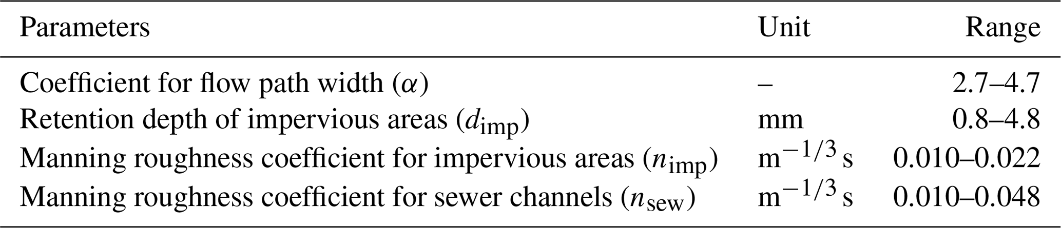
The model uncertainty was estimated using generalized likelihood uncertainty estimation (Beven and Binley, 1992). It was assumed that model uncertainty can be described by the random variability of its calibrated coefficients. The coefficient variability ranges for the SWMM of the Kielce Basin were investigated in previous studies (Kiczko et al., 2018; Szelag et al., 2016). They are shown in Table 1. In the previous studies conducted by Kiczko et al. (2018) and Szeląg et al. (2016), parameter identification was performed along with the Bayesian approach using likelihood functions. The parameters were identified on the basis of Bayesian estimation (Beven and Binley, 1992):

$$\begin{array}{}\text{(6)}& P(Q/\mathit{\theta })={\displaystyle \frac{L(Q/\mathit{\theta })P\left(\mathit{\theta }\right)}{\int L(Q/\mathit{\theta })P\left(\mathit{\theta }\right)d\mathit{\theta }}},\end{array}$$

where P(θ) stands for an a priori (Table 1) calibrated coefficient distribution (uniform distribution was applied in the present study), and $L(Q/\mathit{\theta })$ is a likelihood function used to calculate weights for the Monte Carlo sample depending on the model fit to the observed basin flows Q and $P(Q/\mathit{\theta })$ resulting in a posteriori distribution of model coefficient θ. The following formula was used as the likelihood function (Romanowicz and Beven, 2006):

$$\begin{array}{}\text{(7)}& L(Q/\mathit{\theta })=\exp \left({\displaystyle \frac{{\sum }_{i=\mathrm{1}}^N{\left(Q_i-\widehat{Q_i}\right)}^{\mathrm{2}}}{\mathit{\kappa }\cdot {\mathit{\sigma }}^{\mathrm{2}}}}\right),\end{array}$$

where Q_i and $\widehat{Q_i}$ values represent the time series of observed and computed flows, respectively, and κ is the scaling factor for the variance σ² of model residuals used to adjust the width of the confidence intervals. In the study conducted by Kiczko et al. (2018), the value of κ was determined, ensuring that 95 % of observed flow points are enclosed by 95 % confidence intervals of the model output.

The coefficients in the ranges given in Table 1 were uniformly sampled 5000 times, and the model was evaluated for each set. The simulation goodness of fit was determined as the standard deviation of computed and observed outflow hydrographs. The behavioral simulations were selected using a threshold value of deviation; i.e., simulations with a poorer fit were rejected. The threshold value was determined iteratively to ensure that confidence intervals explained the model uncertainty with respect to the observation. The goal was to enclose 95 % observation points within 95 % confidence intervals. Confidence intervals were calculated on the basis of empirical cumulative distribution functions of an ensemble of modeled hydrographs. The value of the threshold was iteratively increased to reach the above assumption. Coefficients were identified, and the threshold was adjusted for two rainfall events on 24 July 2011 and 15 September 2010. The size of the behavioral set was 5000. It should be noted that it is assumed in the above approach that the simulations from the behavioral set are equally probable. In this study, analyses were limited to four parameters in the SWMM. Computer simulations (Szeląg et al., 2016) using the presented catchment model (SWMM) integrated with the MATLAB algorithms, in which the GLUE+GSA method was implemented (including global sensitivity analysis and uncertainty analysis), showed that the parameters of the Horton model, retention depth, and Manning's roughness coefficient of pervious areas had a negligible impact on the modeled outflow hydrograph from the catchment. These results were also confirmed by simulations performed by other researchers (Thorndahl, 2009; Fu et al., 2011; Fraga et al., 2016) for urban catchments in Belgium, Great Britain, Italy, etc., using local and global sensitivity analytical methods. These results were also confirmed in the analyses performed by Skotnicki and Sowiński (2015) and Mrowiec (2009) for catchments in Poland. The relationships between the calibrated parameters in the SWMM and the modeled parameters of the outflow hydrograph are complex and depend on many factors, i.e., spatial distribution of impervious areas, geometry and retention of the stormwater network, catchment area, etc. (Razavi and Gupta, 2015). Due to the size of the catchment area and limited outflow from pervious areas compared with impervious areas (Szeląg et al., 2016), the roughness and retention coefficients of impervious areas proved that they had a negligible effect on the outflow hydrograph from the catchment compared with other calibrated parameters of the SWMM.

With precise spatial data about the catchment, it was shown that the uncertainty in the identification of impervious areas also had an insignificant influence on the modeled outflow hydrograph (Szeląg, 2014, 2016). Based on the continuous rainfall series from the 2010–2016 period and the determined a posteriori distributions of calibrated coefficients in the SWMM, simulations of the combinations of numerical values [α, n_imp, d_imp, n_sew] (5000 samples) were carried out, which facilitated the determination of catchment outflow hydrographs (Fig. B3, Appendix). On this basis, parameters, i.e., maximum instantaneous outflow (Q_m) and volume (V), were determined for each calculated hydrograph. The results of these analyses were used for the development of logit models for the established threshold values (Q_g,m and V_g) and the assumed temporal rainfall distributions (R1, R2, R3, and R4). To ensure that the number of rainfall events in the 2010–2016 period was 321 rainfall events, 160 5000 rainfall event simulations were performed (considering the uncertainty of the SWMM), of which 120 000 episodes were separated for logit model validation.

3.7 Verification of generated logit models for analysis of hydrograph parameters

The suitability of the generated logit models for simulation tasks in the case of the stormwater catchment analyzed in this study was verified vs. measurement data. Since the temporal rainfall distributions in the rainfall events derived from measurements varied, they were assessed and adjusted to the theoretical distributions presented in this study (see Fig. B1, Appendix B) based on the value of the correlation coefficient (R) expressing the goodness of fit of empirical distributions $\frac{P}{P_{\mathrm{t}}}=f\left(\frac{t}{t_{\mathrm{r}}}\right)$ to the theoretical distributions (R1, R2, R3, and R4).

4 Results and discussion

Following the developed computational algorithm, the “Results and discussion” section includes the following steps: determining the threshold values of the outflow hydrograph parameters using the hydrodynamic model of the catchment, as well as uncertainty analysis; developing the logistic regression model and its verification; sensitivity analysis, in which the influence of rainfall origin and temporal rainfall distribution on the parameters of the hydrograph is analyzed (volume and maximum flow rate); and analysis of the impact of uncertainty of the estimated coefficients in the logit model on the determined sensitivity coefficients.

4.1 Separation of independent rainfall events

Independent rainfall events were distinguished based on a series of rainfall events (2010–2016) measured at the rainfall station located at a distance of 2 km from the Si9 collector catchment and the definition of a rainfall event specified above. The number of events in the individual study years was estimated at 36–58. The rainfall duration (t_r) in the events was 20–2366 min, and the length of the dry period was 0.16–60 d. The rainfall depth (P_tot) in the rainfall events was in the range of 3.0–45.2 mm.

4.2 Establishment of threshold values

The values of calibrated parameters shown in Table 1 served for the SWMM calculations. Assuming rainfall intensity values corresponding to normal (P_tot,u = 3.7 mm), heavy (P_tot,m = 5.8 mm), and torrential (P_tot,g = 21.9 mm) rain, outflow hydrographs were determined for t_r = 15 min, and the Q(t) values were determined at a 10 s resolution. The abovementioned assumption is made because the area under consideration is a small urban catchment, where the time of stormwater runoff is relatively short, and the stormwater retention time is limited due to the significant slope in the channels, reaching 3.9 %. Moreover, the stormwater system model is simplified and limited to the main channels. In the context of the adopted assumptions (catchment retention resulting from land development and topography), the value of the rainfall duration (t_r = 15 min) theoretically including the concentration time, the pipe retention time seems to be representative for small urban catchments, considering that the measure of the influence of rainfall origin on the model sensitivity is primarily to be differentiated by the mean intensity of rainfall (Meynink and Cordery, 1976; Watt and Marsalek, 2013; Krvavica and Rubinić, 2020). Appropriate selection of the duration of rainfall and classification of rainfall for calculation purposes may result from the local rainfall parameters and the climatic conditions shaping the dynamics of rainfall–runoff processes. The simulations revealed the following values of maximum instantaneous flow and hydrograph volumes: Q(q_u)_m = 0.275 m³ s⁻¹ and V(q_u) = 450 m³, Q(q_s)_m = 0.735 m³ s⁻¹ and V(q_s) = 812 m³, and Q(q_g)_m = 2.95 m³ s⁻¹ and V(q_g) = 3500 m³, respectively. It is worth noting that the values of the catchment outflow hydrographs were identical to the rainfall intensity distributions R1, R2, R3, and R4, as demonstrated by Szeląg et al. (2016).

4.3 GLUE

Parameters were identified using outflow time series for two rainfall events on 24 July 2011 and 15 September 2010 (Kiczko et al., 2018). The threshold value of the correlation coefficient ensuring that 95 % of the observations were enclosed within 95 % confidence intervals was 0.920. The size of the behavioral obtained set was 3375. The confidence intervals were verified for two rainfall events on 30 May 2010 and 30 July 2010 (see Fig. B2 – Appendix B). The percentage values of the enclosed observation points were as follows: 91 % for 30 May 2010 and 47 % for 30 July 2010 (Kiczko et al., 2018).

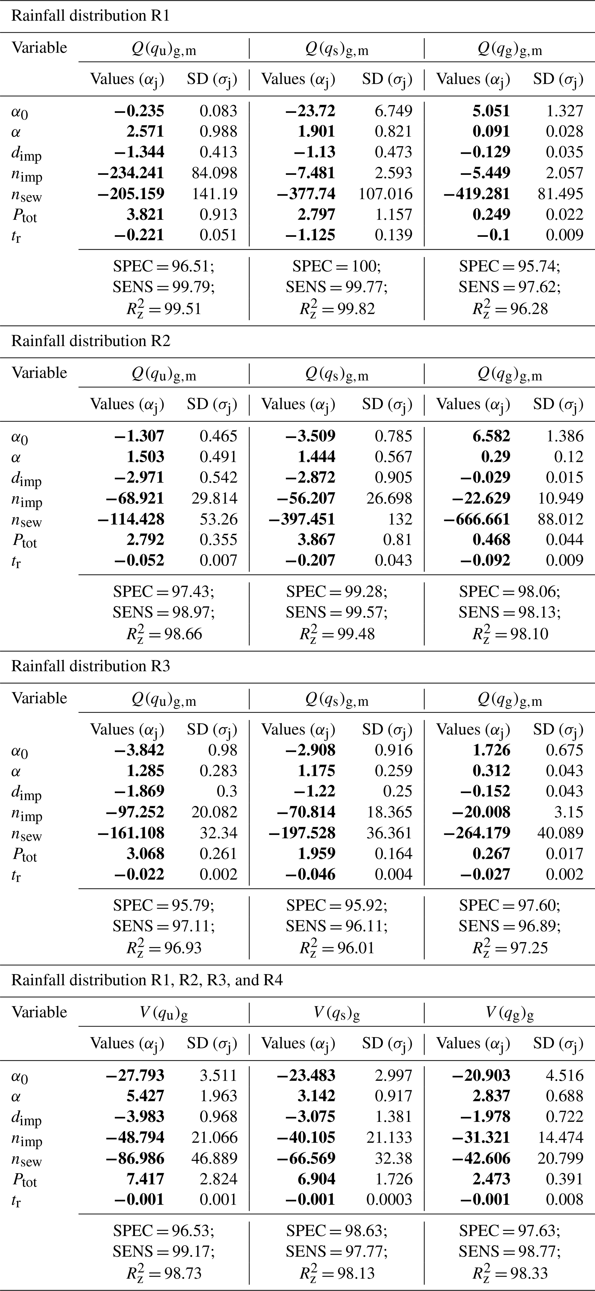
Table 2 Calculated coefficients (α_j) and measures of the goodness of fit of measurement results to the logit model calculations of the Q_g,m and V_g values for rainfall distributions R1, R2, R3, and R4. Statistically significant parameters are in bold.

4.4 Estimation of coefficients in the logit model and assessment of goodness of fit

Based on the determined values of the dependent variables and the corresponding explanatory variables (P_tot, t_r, α, d_imp, n_imp, and n_sew) for the assumed rainfall distributions (R1, R2, R3, and R4), logit models were generated for calculation of the probability of exceeding the threshold values: maximum instantaneous flows (Q_g,m) and outflow hydrographs (V_g). Table 2 presents the determined values of empirical coefficients (α_j) and assessment of the goodness of fit of the calculation vs. measurement results in the logit models used for calculation of p = F(Q_m,g) and p = F(V_g). The calculations indicated identical coefficient values in the case of temporal rainfall distributions R3 and R4 in the logit model; hence, the tables below show the results for temporal rainfall distribution R3. The analysis of the goodness of fit of the calculated results to the measurement results (SPEC, SENS, and $R_{\mathrm{z}}^{\mathrm{2}}$) revealed that the proposed logit models were characterized by satisfactory classification abilities.

Table 3 Results of validation of logit models shown in Table 2.

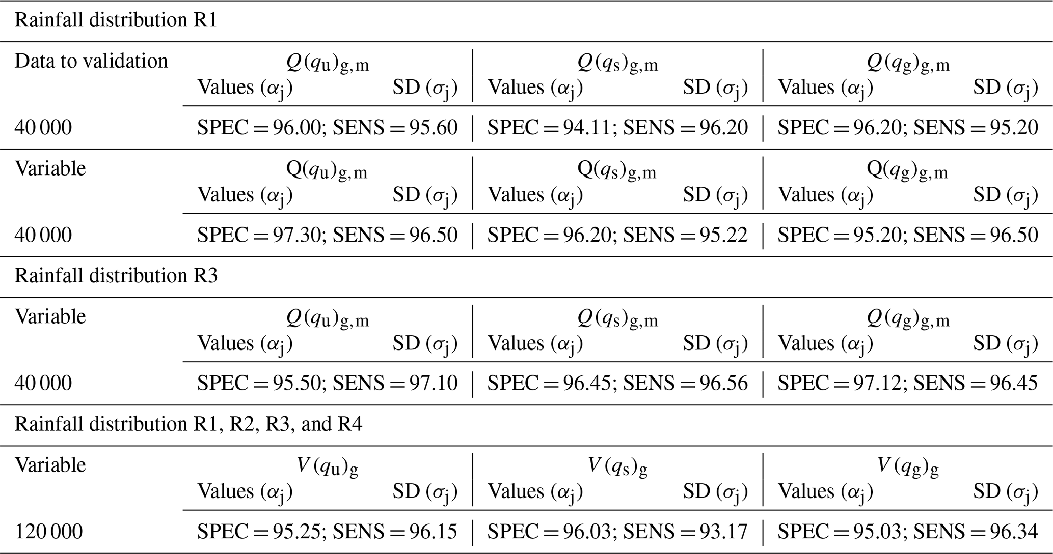
As shown in Table 2, no less than 95.79 % of the cases were correctly identified at the calculated values of p < p(Q_g,m; V_g) and p ≥ p(Q_g,m; V_g). The model was validated with 40 000 independent rainfall events for R1, R2, R3, and R4 rainfall distributions (Table 3).

The results of calculations of the goodness of fit measures of the logit models for the temporal rainfall distributions R1, R2, R3, and R4 associated with the normal, heavy, and torrential rains confirm the high goodness of fit of the calculated and measured results. This confirms the suitability of the models for further analyses.

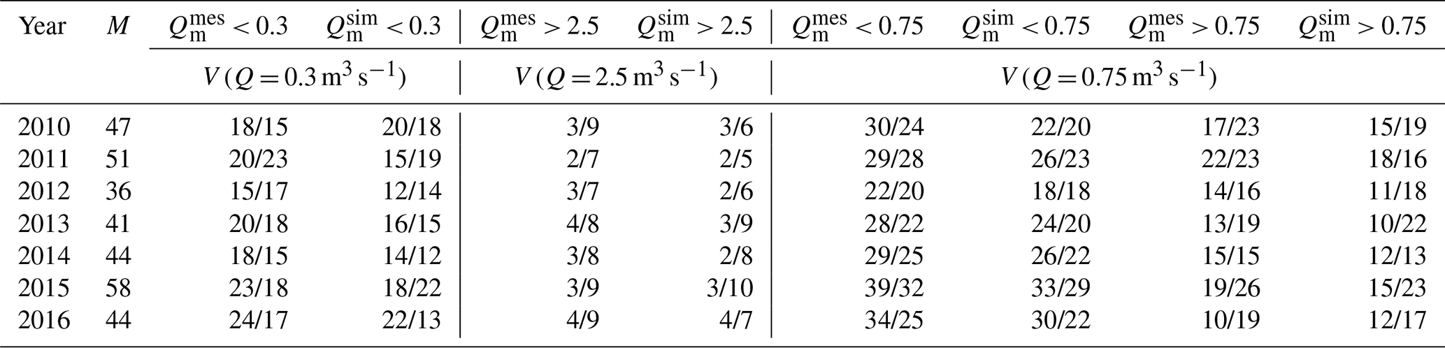
Table 4 Comparison of measurement and calculated results in the analyzed period.

4.5 Verification of the generated logit models vs. measurement data

The analyses showed that in 237 of the 248 events for which the empirical and theoretical rainfall distribution exhibited high convergence (R ≥ 0.96), the calculated results from the logit models were consistent with the simulation data provided by the SWMM in terms of the Q_m classification. In the total number of 248 rainfall events, the R1 temporal rainfall distribution was identified in 126 events (calculated results consistent with measurements in 122 events), 72 events represented the R2 temporal distribution (calculated results consistent with measurements in 69 events), and 58 events were determined as the R3 and R4 temporal distributions (simulation results consistent with measurements in 56 events). In the other 73 events (with R < 0.96), the results of calculations performed in the logit models agreed with the measurement results in 43 events. In this group of events, 19 rainfall events were classified as the R1 temporal distribution (simulation results consistent with measurement results in 8 events), 23 events represented the R2 temporal distribution (calculated results consistent with measurement results in 17 events), and 31 events were identified as the R3 and R4 temporal distributions (simulation results consistent with measurements in 18 events). The V_g value calculated for 321 rainfall events agreed with the measurement results obtained for 281 events. Table 4 shows a comparison of the calculated results provided by the proposed logit models with the measurement results obtained in consecutive years (2010–2016).

The table shows the agreement of the calculated results for the hydrograph parameters obtained via simulation with the SWMM and logistic regression with regard to the classification of maximum flows and hydrograph volumes. The data presented in Table 4 indicate agreement of the logit model-based calculated results with the measurement results.

In Table 4, the format $x_{\mathrm{1}}/x_{\mathrm{2}}$ represents the number of rainfall events in a year with an exceeded x₁ = $Q_{\mathrm{g},\mathrm{m}}/x_{\mathrm{2}}$ = V_g threshold value; calibrated values α, n_imp, d_imp, and n_sew specified in the “Hydrodynamic model” section were used for verification calculations in the logit models shown in Table 4.

The calculated results confirm that the proposed logit models include the key determinants of the variability of hydrograph parameters, which has been confirmed in theoretical studies and the results of field studies conducted by many authors (Gironás et al., 2010; Guan et al., 2015; Thorndahl, 2009). The maximum difference between the number of rainfall events where the parameters of the catchment outflow hydrograph were identified correctly based on rainfall distribution and rainfall characteristics by the logit model and the calibrated values of the SWMM was six events, which was noted for 2015. In this case, and in the other years, this was associated with problems with agreement between empirical and theoretical distributions specified in DWA-A 118E (2006). This was confirmed by the local nature of the dynamics of rainfall events in some urban catchments in Europe, as reported by various authors (De Paola and Ranucci, 2012; Todeschini et al., 2012) investigating the variability of temporal rainfall distribution in a rainfall event. Hence, there is a need to construct regional rainfall models that take into account the variability of measured rainfall distribution in an event rather than that assumed for another region (Wartalska et al., 2020). However, this may be the only solution in the absence of measurement data, which has been confirmed in studies on the use of typical DWA-A 118E (2006) rainfall distributions to model sewer network operation (Siekmann and Pinnekamp, 2011). Analysis of the data compiled in Table 3 demonstrates that, in addition to their theoretical value and the possibility of determining sensitivity (Q_m and V_g), the proposed models can be used for identification of an event with a probability of exceeding the Q_m,g or V_g values in the analyzed catchment.

The analyses performed in this study (Table 2) indicate a strong effect of the flow path width (α), Manning roughness coefficient of impervious areas (n_imp), retention depth of impervious areas (d_imp), and Manning roughness coefficient of sewer channels (n_sew) on the hydrograph volume and maximum instantaneous stormwater stream outflow in the analyzed catchment. This is confirmed by the values of the α_j coefficients. The other explanatory variables (Table 1) are statistically insignificant at the assumed confidence level of 0.05. These findings were confirmed by Barco et al. (2008), Kleidorfer et al. (2009), and Skotnicki and Sowiński (2015), who calibrated hydrodynamic models of catchments in the USA (Santa Monica; area catchment of 217 km²), Australia (Melbourne; area catchments of 37.98 and 89.10 ha), Poland (Poznań; area catchment of 6.7 km²), respectively. The present simulation results confirm the findings reported for larger catchments located in China (Li et al., 2014), where correlation coefficient values and entropy measures were used; the USA (Muleta et al., 2013), where the GLUE method was applied; and Iran (Rabori and Ghazavi, 2018), where the local sensitivity analysis was carried out. The analysis of the values of coefficients α_j in the logit models indicates that only an increase in the flow path width (α) leads to an increase in the probability of exceeding Q_g,m as well as V_g, which is confirmed by the analyses performed by Barco et al. (2008). An inverse correlation was found for the other parameters in the SWMM (n_imp, d_imp, and n_sew). The results of the n_sew simulations relative to Q_g,m and V_g were confirmed by the calculations reported by Barco et al. (2008) and Li et al. (2014). The catchment analyzed by Li et al. (2014) was located in China (Changsha city, area catchment of 11.7 ha). The impervious area accounted for 56 % of the catchment. The increase in the n_sew value reported by many authors (Barco et al., 2008; Fraga et al., 2016; Li et al., 2014) indicated an opposite relationship to that observed in this study. This shows that an increase in the n_sew value results in a shorter stormwater flow time and accumulation of flow from channels, which leads to a rise in the stormwater level and reduction of the instantaneous flow stream in the cross-section closing the catchment (Leandro and Martins, 2016). The calculations performed by Li et al. (2014) confirmed the Q_m = f(n_imp) relationship obtained in this study; however, these analyses did not include the rainfall distribution and genesis. The n_imp and d_imp simulation results obtained in this study are relevant in the nonlinear reservoir SWMM for simulation of the catchment outflow (Gironás et al., 2010; Rossman, 2015). An increase in the catchment retention leads to a reduction in the amount of stormwater flowing into the sewer channels, which has an impact on the simulation results of the outflow in the cross-section closing the catchment.

4.5.1 Sensitivity coefficients – hydrograph volume vs. maximum instantaneous flow

The plotted curves indicated that the smaller the volume of the calibrated catchment outflow hydrograph, the greater the sensitivity of the model to changes in the calibrated coefficients identified in the catchment model (Fig. 5a–d). As part of the present calculations, the effect of the rainfall intensity distribution (ξ) and threshold value (Q_g,m and V_g) on sensitivity coefficients S_xj was assessed. The analyses focused on the temporal R2 distribution, i.e., Euler type II, as this distribution is used for assessment of the effectiveness of the operation of sewer networks (Siekmann and Pinnekamp, 2011) and is thus highly important in engineering considerations. The analyses of the subsequent rainfall distributions (R1, R2, R3, and R4) were based on the maximum flow caused by normal rainfall (Q = 0.3 m³ s⁻¹), which is determined by the occurrence of stormwater overflow in the case of the abovementioned value. The results of these analyses are presented in Figs. 4 and 5.

The analysis of the results of calculations of the probability of exceeding the threshold values V_g revealed that the rainfall intensity distribution did not influence the model sensitivity, which was confirmed by simulation experiments in the analyzed urban catchment (Szelag et al., 2016). The plotted curves (Fig. 5) indicated that the calibrated volume in the domain of the V_g value exhibits the greatest sensitivity (deterministic solution) to changes in d_imp and α. This relationship was confirmed by Skotnicki and Sowiński (2015), who simulated outflows from a 6.7 km² catchment in Poznań and employed local sensitivity analysis. Similar results were also obtained by Rabori and Ghazavi (2018) in their analyses of a catchment outflow in Iran. These correlations were also confirmed by the calculations reported by Mrowiec (2009), who modeled hydrographs in the urban catchment in Częstochowa (120 ha). The present analytical results were also confirmed by Ballinas-Gonzáles et al. (2020), who demonstrated a major impact of the characteristics of impervious areas on the variability of the catchment outflow hydrograph. Different sensitivity analytical results were reported by Li et al. (2014), who demonstrated a crucial effect of n_sew on the outflow hydrograph volume. Among the explanatory variables considered in this study (for any p in Eq. 4), n_imp was found to exert the lowest effect on the probability of exceeding V_g at any p value. The course of the curves and their variability (Fig. 5) indicate the lowest S_xi values of the calibrated coefficient (α, n_imp, d_imp, and n_sew) catchment outflow hydrographs in the case of torrential rainfall events, whereas the highest values were noted in the case of normal rainfall events (on the Chomicz scale). In terms of the selection of hydrographs for calibration followed by validation (SWMM), the present results have an engineering aspect. This is associated with the fact that different relationships V(Q) = f(x_i) can be obtained by validation of the model coefficients at the calibration stage, which is crucial for minimization of the difference between measurement and simulation values.

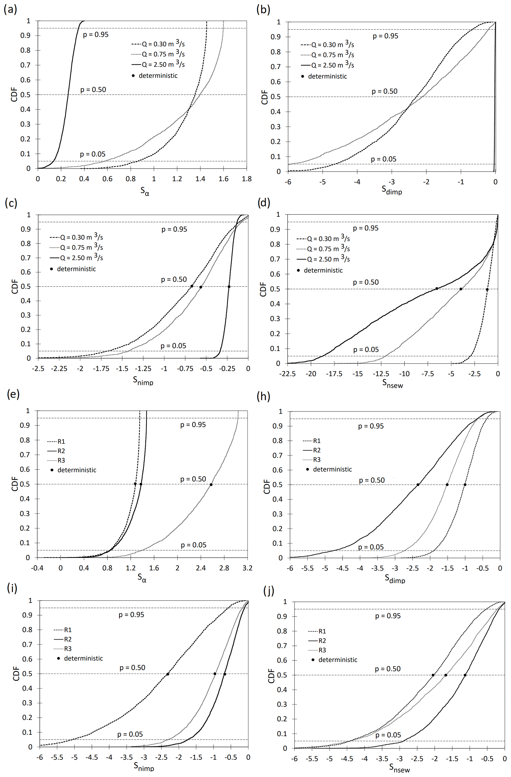
Figure 4 Comparison of the calculated results (deterministic and probabilistic solutions) of sensitivity coefficients (S_α, S_dimp, S_nimp, and S_nsew) for (a–d) threshold values (Q = Q_g,m) and temporal rainfall distribution ξ = R2 and (e–h) temporal rainfall distributions (ξ = R1, R2, and R3) for Q_g,m = 0.30 m³ s⁻¹.

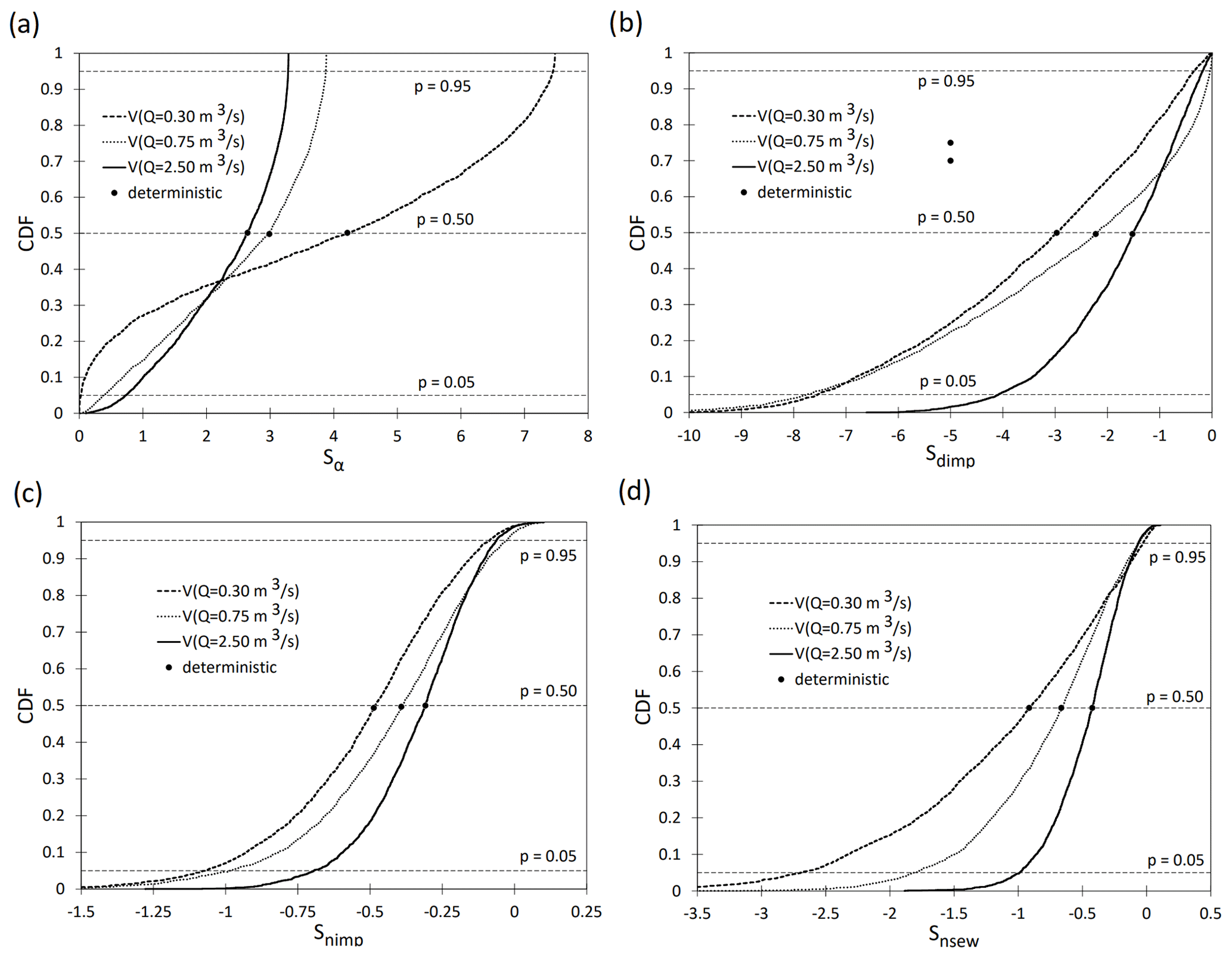
Figure 5 Comparison of the calculated results (deterministic and probabilistic solutions) of sensitivity coefficients (S_α, S_dimp, S_nimp, and S_nsew) for threshold values V(Q) = V_g and temporal rainfall distribution ξ = R1, R2, and R3.

The curves in Fig. 4e–h show that apart from the rainfall origin (average rainfall intensity as a result of normal, heavy, and torrential rainfall), the temporal distribution of rainfall has an impact on the values of the determined sensitivity coefficients. This result is the effect of the fact that the temporal distribution of rainfall and the intensity of rainfall have a significant impact on the values of the modeled maximum flow rates, which was confirmed by the analysis by Schilling (1991). The obtained curves (Fig. 5) prove that the volume of the outflow hydrograph depends on the origin of rainfall and hence the variability of the determined values of the sensitivity coefficients for normal, heavy, and torrential rainfall.

In turn, the impact of rainfall distribution was not found, which was confirmed by studies in the field of modeling the volume of runoff from urban catchments (Grum and Aalderink, 1999), including computer simulations by Szeląg et al. (2014) for the urban catchment under consideration.

4.5.2 Sensitivity coefficient – maximum instantaneous flow vs. rainfall distribution

Based on the plotted curves (probabilistic solution), it can be concluded that when the Q_m value is calibrated in the region of Q_g,m = 0.30 m³ s⁻¹ (uniform rainfall distribution R1, normal rain), the model shows the greatest sensitivity (percentile 0.50) to changes in n_imp (deterministic solution), as confirmed by the value S_nimp = −2.47 (Fig. 4g). The Manning roughness sewer channel coefficient (S_nsew = −2.12; Fig. 4h), flow path width (S_α = 1.25; Fig. 4e), and retention depth of impervious areas (S_dimp = −1.03; Fig. 4f) have a lower impact. The plotted curves and the deterministic solution indicate that the absolute S_nimp and S_nsew values for the R2 and R3 temporal rainfall distributions (deterministic solution) are lower than those for the R1 distribution (Fig. 4e–f). In turn, in the case of S_α (Fig. 4e) and S_dimp (Fig. 4f), it was found that the absolute values of the sensitivity coefficients calculated for the R1 distribution have lower values than for R2 and R3. When the model is calibrated based on hydrographs reflecting the reaction of the analyzed catchment to normal rain (constant temporal rainfall distribution in an event – R1), the greatest effect on the Q_m in the Q_g,m domain is exerted by n_imp and the lowest impact is shown by d_imp (in terms of absolute values); this is indicated by the curves in Fig. 4f–g. In turn, a different relationship, i.e., the greatest effect of d_imp and α and the lowest effect of n_imp, was found for the R2 distribution (Fig. 4e and f). These relationships indicate a significant effect of temporal rainfall intensity distributions on the model sensitivity to changes in the coefficients calibrated in the domain of Q_g,m values.

The results of the present analyses may be highly important in engineering practice, as they confirm that, with the Q_m values assumed to be the basis for calibration, the hydrograph should be selected in a way that facilitates identification of the coefficients (α, d_imp, n_imp, and n_sew) and validation so that the values will be a result of rainfall with similar intensity dynamics. Therefore, it should be emphasized that in the hydrograph intended for identification of model coefficients and validation, the relationship between the dependent variables and the calibrated coefficients must have a similar form.

4.5.3 Sensitivity coefficients – maximum instantaneous flow vs. size of threshold Q_m

The plotted curves (probabilistic solution) with the deterministic solutions showed that the greater the rainfall intensity (rising Q_m value), the smaller the values of the sensitivity coefficients (S_α, S_nimp, and S_dimp) (Fig. 4a–d). This indicates a decline in the sensitivity of the model of predicting the probability of exceeding Q_g,m to changes in calibrated parameters (α, n_imp, and d_imp) (Fig. 4a–c). An inverse relationship was found for the n_sew value (Fig. 4d). During the calibration of the catchment model for normal rainfall (maximum intensity in the middle of the event – R2), the model exhibited the highest sensitivity (Q_g,m prediction) to changes in the retention of impervious areas (S_dimp = −2.342; Fig. 4b) and the lowest sensitivity to the Manning roughness coefficient of impervious areas (S_nimp = −0.683; Fig. 4c). In the case of calibration of the catchment model for heavy and torrential rainfall events, the maximum instantaneous flow Q_m in the region of corresponding Q_g,m values exhibited the highest sensitivity to changes in n_sew (Fig. 4d).

The relationships presented in this study have been scarcely analyzed by other researchers (Barco et al., 2008; Krebs et al., 2014; Li et al., 2014) in terms of catchment outflow modeling. These relationships, which confirm the significant effect of rainfall intensity distribution on hydraulic phenomena occurring in a sewer network, were described by Jato-Espino et al. (2018) in their study of stormwater overflow. The authors showed a statistically significant effect of the rainfall intensity distribution on the relationship between stormwater overflow onto the land surface and catchment characteristics. A certain analogy with the calculated results described in the present study may be suggested. This is related to the fact that, along with the increase in rainfall intensity, Jato-Espino et al. (2018) reported a decline in the sensitivity of the model to the values of selected catchment characteristics; this is equivalent to a decrease in the sensitivity of the model to the calibrated parameters.

4.5.4 Sensitivity coefficients – uncertainty of estimated coefficients in the logit model

The calculations showed that the uncertainty of parameter estimation in logit models exerts a strong effect on the values of the sensitivity coefficients calculated for the analyzed cases. This is confirmed by the determined range of variability of the sensitivity coefficient values (S_α, S_nimp, S_dimp, and S_nsew) depending on the size of the respective percentiles (Figs. 4 and 5). In most calculation variants (with the exception of α; Figs. 4a and e and 5a), the difference between the determined values of the sensitivity coefficients (for the different temporal rainfall distributions R1, R2, and R3 – normal, heavy, and torrential rains, respectively, and rainfall genesis) was shown to decrease with the increase in percentile values.

Different relationships were observed in the analysis of the variability of S_xi values shown in Fig. 5a. In this case, for percentiles below 0.36, the highest and lowest S_α values were obtained for V(Q_m,g = 2.50 m³ s⁻¹) and V(Q_m,g = 0.30 m³ s⁻¹), respectively. The analysis of the effect of rainfall distribution (R1, R2, and R3) on model sensitivity (calibrated Q_m value) revealed an increase in the difference in the sensitivity coefficient S_α values with the increase in the percentiles. As shown by the analysis of the values of sensitivity coefficients S_α and S_dimp (Fig. 4a and b), the relationship S_α(dimp)(Q_m = 0.75 m³ s⁻¹) > S_α(dimp)(Q_m = 2.50 m³ s⁻¹) was obtained for percentile values above 0.42, whereas an inverse relationship was found for lower percentile values.

5 Summary and conclusions

Modeling of outflows and calibration of hydrodynamic models with the design of tools supporting this task represent a relevant current research topic. It is necessary to search for methods that will yield reliable results reflecting reality, as well as what is possible, on the one hand. On the other hand, with their acceptable time and cost efficiency in the retrieval and analysis of data, the methods should have the potential to be used in practice by a wide group of engineers. The currently used methods of analyzing the sensitivity of hydrodynamic models neglect the origin of rainfall and the temporal distribution of rainfall. Moreover, in the methods based on statistical models, the influence of the uncertainty of the estimated coefficients in the logit model on the values of the calculated sensitivity coefficients is not taken into account. Neglecting the abovementioned conditions may result in problems with the calibration of models and simplification in the interpretation of the physics of hydrological processes in catchments, which makes them difficult to understand. This study showed that the logistic regression model can be used for analyses of the sensitivity of the maximum flow in a hydrograph and hydrograph volume in a rainfall event. The hydrograph parameters depended on the temporal rainfall intensity distribution in the rainfall event and parameters identified in the SWMM. In addition to their scientific aspects, the proposed logit models may be a useful tool for forecasting the variability of the parameters of catchment outflow hydrographs, which confirms the usefulness of the developed tool. The analyses performed in this work showed that the origin of rainfall and the temporal distribution of rainfall in the event have a large impact on the sensitivity of the model. However, this aspect has been neglected until now in sensitivity analytical methods. The results of the calculations showed that the lowest values of the sensitivity coefficients were obtained for the outflow hydrographs resulting from heavy rainfall, while the highest values of the sensitivity coefficients were obtained for normal rain. In the context of the currently used methods of sensitivity analysis and calibration, it seems advisable to modify them by introducing an additional calculation step consisting of the classification of the measured rainfall data in terms of the origin of rainfall (accounting for average rainfall intensity) and the temporal distribution of rainfall. For this purpose, it is possible to use unsupervised machine learning methods (hierarchical cluster analysis, Kohonen neural networks, etc.). In the context of the obtained calculated results, it is advisable to select the rainfall–runoff events for calibration and validation in such a way that the determined sensitivity coefficients do not show significant variability. It is important for the appropriate selection of the values of calibrated parameters and their potential correction at the stage of model validation. The sensitivity coefficient proposed in this study facilitates the determination of the impact of selected parameters of the SWMM on the outflow hydrograph parameters with consideration of rainfall genesis and variability of temporal rainfall distribution in a rainfall event. Furthermore, it was demonstrated that rainfall genesis and the temporal variability of rainfall intensity in a rainfall event should be included in the selection of hydrographs for calibration and validation of the model. It was found that the higher the rainfall intensity determining the modeled outflow hydrograph, the lower the sensitivity of the identified SWMM parameters to the maximum outflow and hydrograph volume. The calculations indicated that the uncertainty of the coefficients identified in the logit model has a significant impact on the determined sensitivity coefficients. The aspects discussed above are highly important for the procedure of hydrodynamic model calibration, which ultimately has a significant effect on the accuracy of the identified model parameters.

The computational methodology proposed in this paper is universal in nature and can be applied to any urban catchment area. The simulation results presented in this paper refer to a single catchment area. Therefore, further analyses are required to verify the developed model for catchments with different physical and geographic characteristics. Thus, it is advisable to determine the applicability range of the developed computational model. Considering the usefulness of the obtained dependencies, as well as the large influence of rainfall origin and rainfall temporal distribution on the sensitivity coefficients, further studies are needed. The purpose of these analyses should be to expand the developed methodology of the sensitivity analysis aimed at additionally taking into account the shape and area of the catchment, land use, the path of the stormwater network, and the retention of the network. The analysis of the effect of the temporal distribution of rainfall, together with the spatial distribution, seems to be a particularly interesting issue, especially because both distributions strongly depend on rainfall genesis. However, the design of an appropriate experiment seems challenging.

Appendix A: List of symbols

tr	rainfall duration,
Ptot	rainfall depth,
αj	estimated coefficient of logistic regression model,
α0	rainfall efficiency coefficients taking into account the normal, heavy, and torrential rain types,
qu	hydrograph caused by normal rainfall (according to the Chomicz scale),
qs	hydrograph caused by heavy rainfall (according to the Chomicz scale),
qg	hydrograph caused by torrential rainfall (according to the Chomicz scale),
R1, R2, R3, and R4	temporal rainfall distribution,
V	volume of hydrograph,
Qm	maximum instantaneous flow,
Vg	threshold of volume of hydrograph,
Qg,m	threshold of maximum instantaneous flow,
ξ	function describing the temporal intensity distribution,
nimp	Manning roughness coefficient for impervious areas,
nsew	Manning roughness coefficient for sewer channels,
α	coefficient for flow path width,
GLUE	generalized likelihood uncertainty estimation,
dimp	retention depth of impervious areas,
Sxj	sensitivity coefficient,
p	probability of exceeding of Qg,m and Vg,
SWMM	Storm Water Management Model,
SPEC	specificity,
SENS	sensitivity,
$R_{\mathrm{z}}^{\mathrm{2}}$	calculation error,
ε	empirical coefficient for conversion of the $Q_{\mathrm{m}}^{\ast }$ value into p∗,
Q(t)	outflows from of the catchment at time t,
$x_{\mathrm{1},\mathrm{2},j=n}$	calibrated parameters in the SWMM.

Appendix B: Supporting graphical information

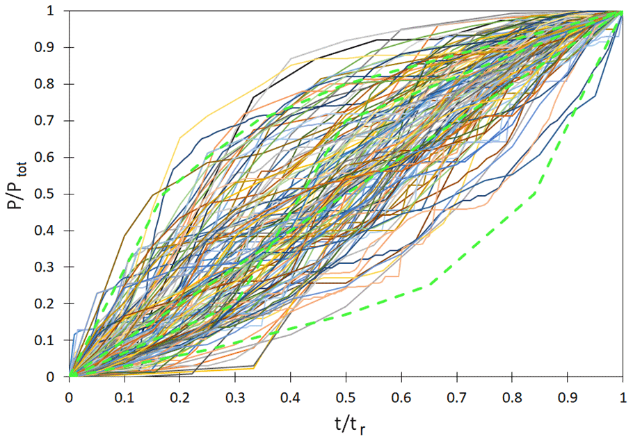
Figure B1 Dimensionless rainfall curves, $P/P_{\text{tot}}$ = $f(t/t_{\mathrm{r}})$, obtained from measurements performed in 2008–2016.

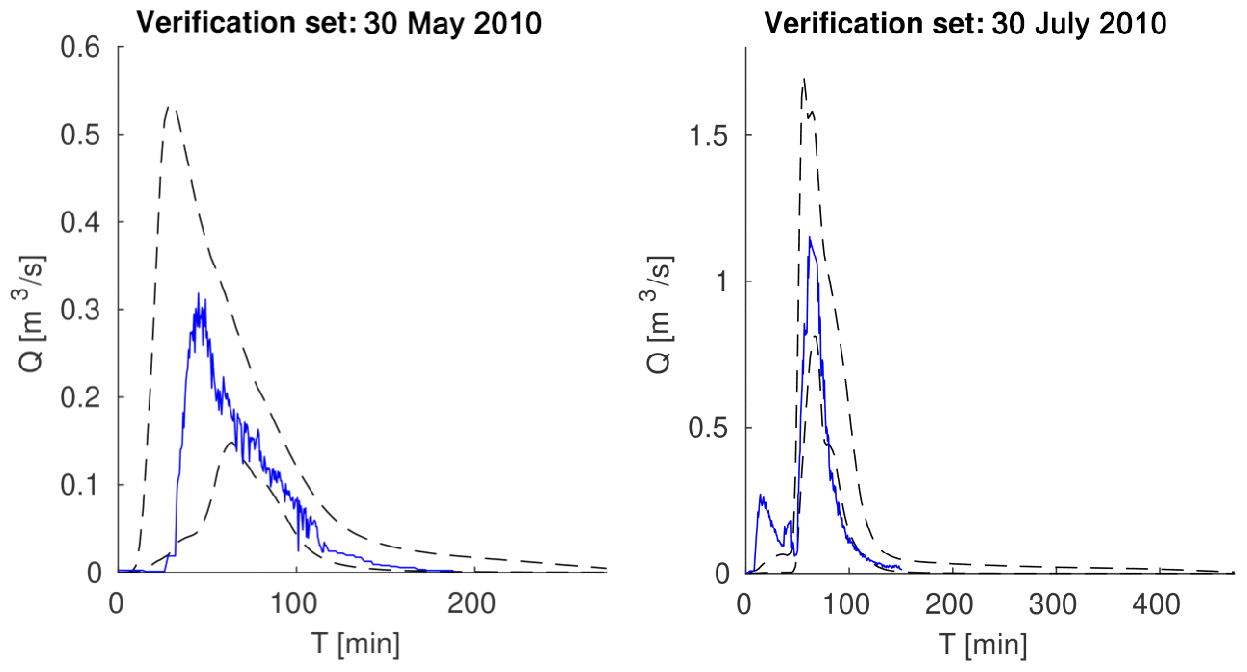
Figure B2 Comparison of measurement results of hydrographs of outflow from the catchment area with GLUE calculations.

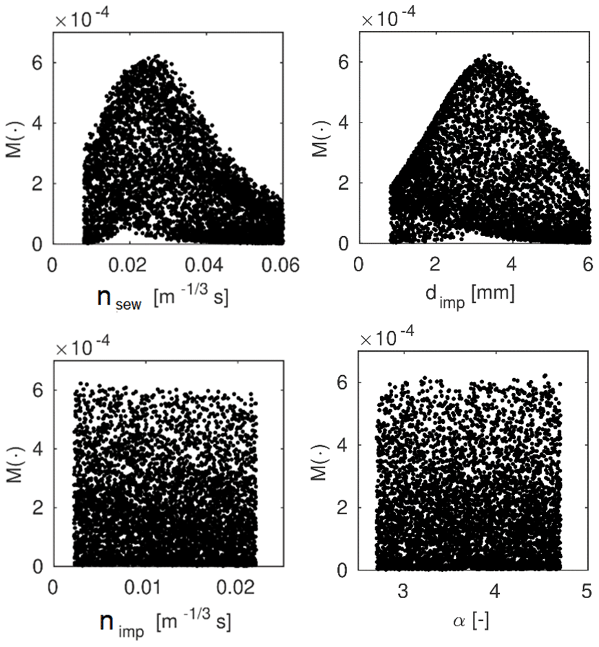
Figure B3 Calculated likelihood function – scatter plots of M values versus calibrated catchment parameters in SWMM.