Bridging the scale gap: obtaining high-resolution stochastic simulations of gridded daily precipitation in a future climate

Climate change impact assessment related to floods, infrastructure networks, and water resource management applications requires realistic simulations of high-resolution gridded precipitation series under a future climate. This paper proposes to produce such simulations by combining a weather generator for high-resolution gridded daily precipitation, trained on a historical observation-based gridded data product, with coarser-scale climate change information obtained using a regional climate model. The climate change information can be added to various components of the weather generator, related to both the probability of precipitation as well as the amount of precipitation on wet days. The information is added in a transparent manner, allowing for an assessment of the plausibility of the added information. In a case study of nine hydrological catchments in central Norway with the study areas covering 1000–5500 km², daily simulations are obtained on a 1 km grid for a period of 19 years. The method yields simulations with realistic temporal and spatial structures and outperforms empirical quantile delta mapping in terms of marginal performance.

1 Introduction

The rate of projected future warming in northern Europe is amongst the highest in the world, driven to a large extent by the strong feedback involving snow and ice as the climate warms (Collins et al., 2013). As a consequence, the hydrological cycle intensifies (Bengtsson, 2010), leading to more precipitation as well as more intense extreme events (e.g. Vautard et al., 2014). The projected changes in precipitation amounts, snowpack, and snow cover will considerably impact surface hydrology through, for example, changed runoff magnitude as well as timing and amplitude of the spring flood (e.g. Von Storch et al., 2015). In order to study these effects, impact models optimally require inputs that reliably represent precipitation occurrence and intensity at a high spatial resolution, spatial and temporal variability, as well as physical consistency for different regions and seasons (Maraun et al., 2010).

Coupled atmosphere–ocean general circulation models (GCMs) remain our main source of information for projections of future climate. However, these have spatial resolutions that are too coarse for assessing the often localized impacts of changing precipitation patterns. Regional climate models (RCMs) at a spatial resolution of 10–15 km (e.g. Jacob et al., 2014) are able to explicitly resolve mesoscale atmospheric processes and add valuable information for precipitation modelling over a region, with the newest model generations at an even higher resolution and able to include explicit deep convection (Lind et al., 2020; Prein et al., 2020).

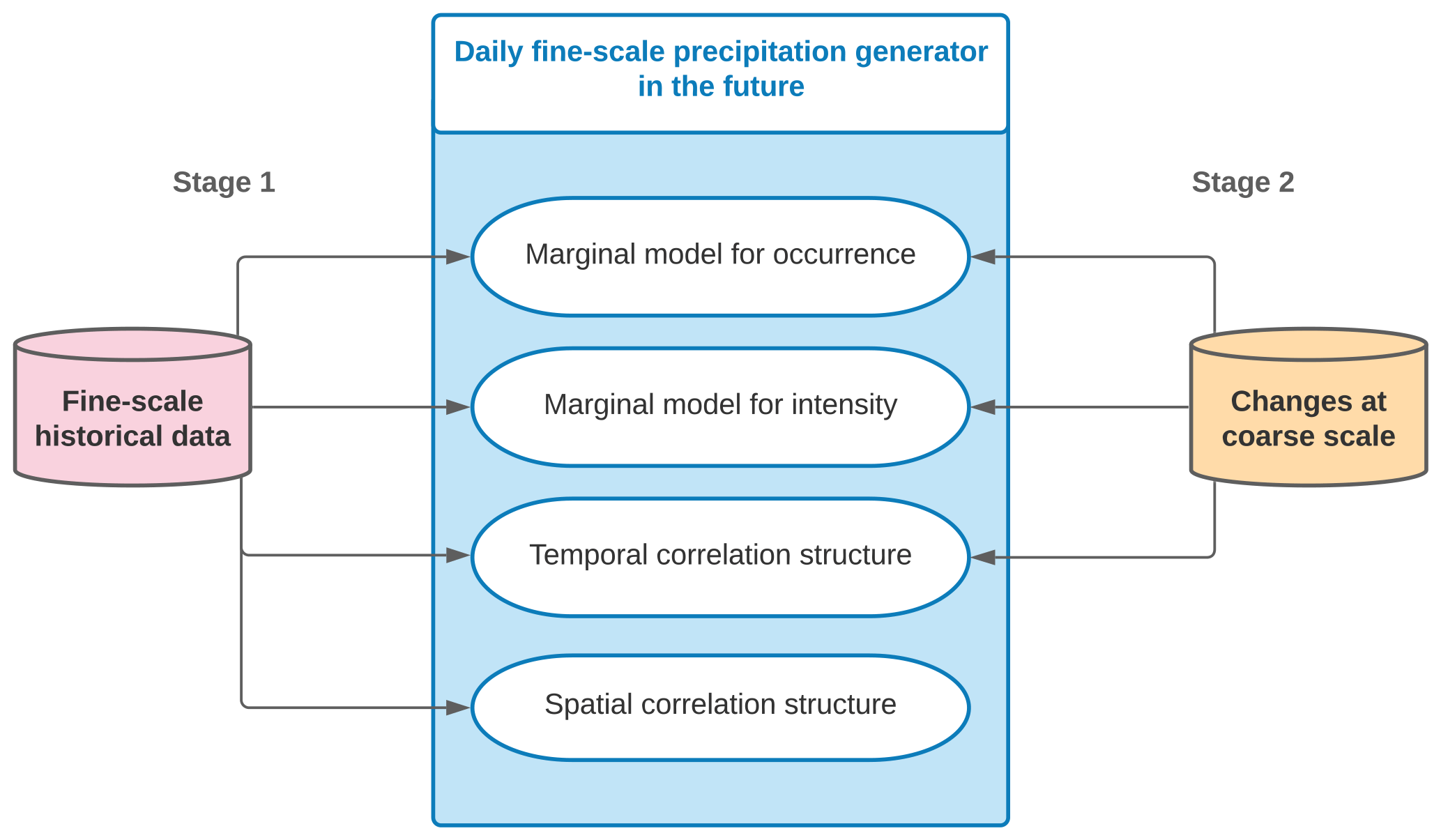
Figure 1 The proposed two-stage weather generator approach for simulations of fine-scale daily precipitation in a future climate.

To obtain reference results for the current climate, impact models are commonly applied to high-resolution historical data products such as the Nordic Gridded Climate Dataset (NGCD, https://surfobs.climate.copernicus.eu/dataaccess/access_ngcd.php, last access: 27 March 2019), which provides historical estimates of precipitation and temperature in northern Europe at a 1 km spatial resolution. Such data products come with their own inherent biases which can be difficult to correct due to lack of data. For an accurate assessment of climate impact, one goal is thus to generate high-resolution realizations of future climate with the same distributional properties as the historical data product, except for potential changes in these distributional properties due to climate change. For comparable future projections, RCM simulations need a further downscaling step, and systematic biases as well as incompatibilities between the two spatial scales should be removed. It has further been argued that downscaling should be stochastic in nature and able to generate sub-grid spatial variability (Maraun et al., 2017). The stochastic point processes of the Neyman–Scott and Bartlett–Lewis types have been used to stochastically downscale precipitation data, most often at single locations (Burton et al., 2008). More recent model extensions into two-dimensional space (Cowpertwait et al., 2002), spatial nonstationarity (Burton et al., 2010), and temporal nonstationarity regarding long-term trends (Luca et al., 2020) have seen rarer applications in the literature. Recently proposed stochastic downscaling methods have proven skillful in modelling the small-scale variability of precipitation occurrence and intensity across sets of point locations (Wong et al., 2014; Volosciuk et al., 2017).

This paper proposes a two-stage weather generator (WG) approach to generate high-dimensional simulations of future climate on a fine-scale grid. Specifically, a stochastic model describing a high-resolution data product in a reference period is combined with climate change projections based on a lower-resolution RCM. Weather generators are commonly used to generate spatially and temporally correlated fields of daily precipitation, with the early work of Wilks (1998) paving the way for many current approaches. Chandler and Wheater (2002) illustrate the use of a generalized linear model (GLM) to describe daily precipitation series at individual sites, using a logistic regression model for the occurrence and a gamma model for the amounts. More recently, Kleiber et al. (2012) propose an approach relying on two latent Gaussian random fields to generate spatially correlated occurrence and intensity, with spatial heterogeneity described through both spatially varying covariates and regression parameters. Serinaldi and Kilsby (2014) propose a more computationally efficient approach, where a single latent Gaussian random field is used to describe the spatial correlation in both precipitation occurrence and intensity.

With applications related to hydrological impacts in mind, we consider a case study of nine different catchments in central Norway. The simulation of daily fine-scale precipitation for a catchment requires daily simulations of spatially correlated random fields on a high-resolution grid with roughly 1000–5500 grid cells, depending on the size of the catchment. As the catchments are located in different climatic zones, the stochastic model is estimated independently for each catchment. Spatial heterogeneity within a catchment is introduced via spatially varying covariates for both the occurrence and the intensity models, where the covariate contribution to the precipitation intensity may vary smoothly in space. Additionally, temporal aspects are modelled with seasonal effects and linear trends in the marginal distributions as well as an autoregressive component in the residual process. Climate change information from an RCM output may be added in a transparent manner by updating each component of the weather generator based on estimated climate change in the corresponding component at the coarser RCM scale. Yuan et al. (2019) propose a similar model for obtaining high-resolution daily mean temperature projections.

As demonstrated in Fig. 1, the stochastic model generates realizations of future precipitation occurrence and intensity that are correlated in space and time, thus combining four separate components: spatial and temporal correlation structures and marginal models at each grid-cell location for probability of occurrence and intensity. The fine-scale spatial correlation structure is assumed constant over time, while climate change information from the RCM can be used to update the other three components in terms of both overall level as well as seasonal patterns. In addition to being stochastic in nature, the method provides a transparent way to add a climate change signal to the precipitation simulations. The success of the model producing realistic realizations for a future climate depends on two factors: the RCM must be able to correctly capture the climate change signal in the model components and the scale of the fine-scale change must be close enough to that of the RCM scale for climate change effects to be transferrable between the two scales.

The remainder of the paper is organized as follows. Section 2 introduces the datasets and the study area. Details of the two-stage WG approach are given in Sect. 3 together with a description of a reference method based on empirical quantile delta mapping as well as the evaluation methods used to compare the two approaches. The models are estimated based on data from the period 1957–1986 and the estimates are used to simulate data for the period 1987–2005. The results of this analysis and comparison of the various approaches are given in Sect. 4. The paper then concludes with a brief summary and discussion in Sect. 5.

2 Data and study area

We apply our methodology to daily precipitation simulations from two RCMs from the EURO-CORDEX-11 ensemble. One (referred to as RCM1 in the following) combines the COSMO Climate Limited-area Model (CCLM) from the Potsdam Institute for Climate Research (Rockel et al., 2008) with boundary conditions from the CNRM-CM5 Earth system model developed by the French National Centre for Meteorological Research (Voldoire et al., 2013), whereas the other (referred to as RCM2) combines the CCLM model with boundary conditions from the MPI Earth system model developed by the Max Planck Institute for Meteorology (Giorgetta et al., 2013). The RCM simulations are conducted over Europe at a spatial resolution of 0.11^∘ or about 12 km (Jacob et al., 2014). In the historical period up to 2005 the outputs are simulated based on recorded emissions and are thus comparable to observed climate.

For observational reference data, we use the seNorge gridded data product version 2018 produced by the Norwegian Meteorological Institute (Lussana et al., 2019) as a subset of the Nordic Gridded Climate Dataset for Norway. The data result from a multi-scale spatial interpolation of measurements from 500 to 700 surface weather observation stations for the period 1957 to the present. The data have a daily temporal resolution and a spatial resolution of 1 km over an area covering the Norwegian mainland and an adjacent strip along the Norwegian border. Compared with previous versions of the data product (i.e. Lussana et al., 2018), seNorge version 2018 adjusts the measurements for wind-induced undercatch of solid precipitation and makes use of dynamically downscaled reanalysis to form the reference fields for data-sparse areas and thus is considered to have a higher effective resolution. In the following, we will treat this dataset as observations and refer to it as such.

Grid-cell precipitation is an areal average of sub-grid precipitations and, at a daily timescale, each value in a time series is an accumulation over 24 h. We upscale the fine-scale seNorge values to the coarse-scale RCM grid by calculating the weighted average over all seNorge grid cells within a given RCM grid cell, where the weights equal the proportion of each seNorge cell within the given RCM cell. The precipitation data have unit kg m⁻², which is approximately equivalent to mm; we then set all values less than 0.1 to 0 before other processing.

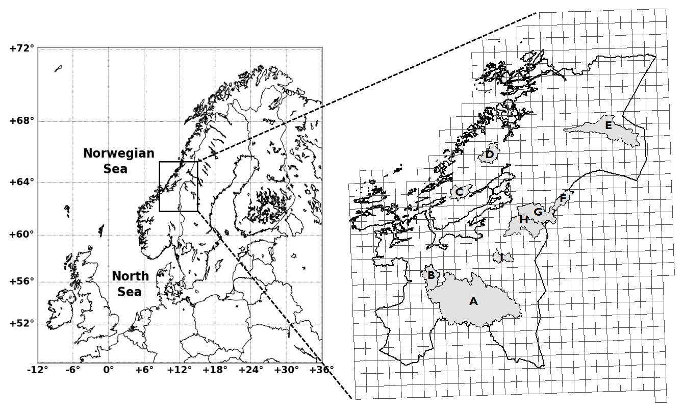
Figure 2 The study area is located in Trøndelag in central Norway, covering the entire Trøndelag and a small part of neighbouring Sweden, and consists of 695 RCM grid cells (rectangular-like polygons) and 109 514 seNorge grid cells (within the polygons, not shown). For stochastic simulations of gridded daily precipitation, nine catchments within Trøndelag with catchment areas from 144 to 3084 km² (shaded in grey) are used; see also Table 1.

Table 1 Characteristics of the nine catchments in Trøndelag, Norway, considered in the stochastic simulations of gridded daily precipitation.

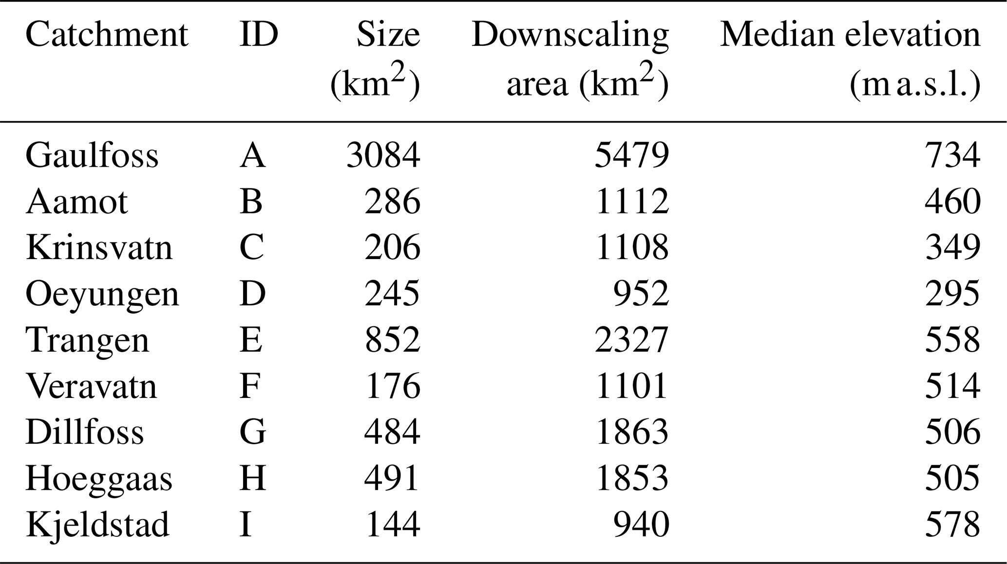
For the study area, we consider the Trøndelag area in central Norway; see Fig. 2. The area comprises 695 RCM grid cells and 109 514 seNorge grid cells. The extraction of the climate change signal is performed at the RCM scale, while the fine-scale daily precipitation fields are generated at nine hydrological catchments within the domain; see Fig. 2 and Table 1. Two of the catchments, Krinsvatn and Oeyungen, have a maritime climate, while the others have a continental climate. For each catchment, the modelling is performed over all seNorge grid cells within the RCM grid cells that cover the catchment, the spatial dimensions of which vary between approximately 940 and 5500 grid cells at 1 km resolution. Both historical RCM simulations and seNorge observations are available over the time period 1957–2005. We use the time period 1957–1986 as a training period to estimate model parameters and perform an out-of-sample evaluation over the remaining 19 years 1987–2005. As a result, the training period consists of 10 950 d, while the test period comprises 6935 d.

Additionally, we use explanatory variables, or covariates, to describe the spatial variations in the statistical characteristics of the daily precipitation distributions. We consider latitude, longitude, and elevation as potential geographic covariates. Elevation information for the seNorge data is obtained from a digital elevation model based on a 100 m-resolution terrain model from the Norwegian Mapping Authority (Mohr, 2009). We upscale these data in the same manner as the daily mean precipitation to obtain the elevation at the RCM scale. Note that this is not equal to the orography information provided by EURO-CORDEX.

3 Methods

As mentioned in the introduction, the aim of this study is to provide realistic projections of daily precipitation at a fine spatial scale over large areas. We apply a parametric weather generator approach that belongs to the class of models proposed by Wilks (1998) and Chandler and Wheater (2002). For computational feasibility, we apply the approach proposed by Serinaldi and Kilsby (2014), where a discrete-continuous distribution with a single latent field is used to simultaneously model the marginal precipitation occurrence, intensity on wet days, and the space–time dependence. Specifically, we employ a combination of a latent non-stationary Gaussian space–time random field and a gamma distribution with parameters that vary in space and time, with each model component estimated independently. The precipitation process at the RCM scale is described using a similar statistical model, and the climate change signal is added to the fine-scale model by relating the models at the two spatial scales.

3.1 Marginal models for precipitation occurrence and intensity

Denote precipitation occurrence in grid cell $s\in \mathit{\{}\mathrm{1},\mathrm{2},\mathrm{\dots },S\mathit{\}}$ at time $t\in \mathit{\{}\mathrm{1},\mathrm{2},\mathrm{\dots },T\mathit{\}}$ by O_st=1 if there is precipitation and O_st=0 otherwise, where S denotes the number of grid cells and T the number of days in a given dataset. We follow Kleiber et al. (2012) and relate the pattern of wet and dry days to a latent Gaussian variable W_st with mean μ_st and variance 1. Precipitation intensity Y_st (i.e. the amount conditional on O_st=1) is assumed to be gamma distributed with a constant shape k and scale θ_st that varies over space and time, following e.g. Chandler and Wheater (2002) and Yang et al. (2005). Formally, we write

$$\begin{array}{}\text{(1)}& {\displaystyle }{W}_{\text{st}}={\mathit{\mu }}_{\text{st}}+{\mathit{\epsilon }}_{\text{st}},{\mathit{\epsilon }}_{\text{st}}\sim N(\mathrm{0},\mathrm{1}),\text{(2)}& {\displaystyle }{O}_{\text{st}}=\text{𝟙}\mathit{\{}{W}_{\text{st}}>\mathrm{0}\mathit{\}},\text{(3)}& {\displaystyle }{Y}_{\text{st}}|O_{\text{st}}=\mathrm{1}\sim \mathrm{\Gamma }(k,{\mathit{\theta }}_{\text{st}}).\end{array}$$

Precipitation processes often show different features depending on the time of the year, and neighbouring sites tend to share a similar precipitation climate. Such systematic variations are modelled by letting the parameters μ_st and θ_st of the above distributions change smoothly across time and space. We describe this through three additive components: a spatial effect, a seasonal effect, and a linear climate change effect. In particular, we set

$$\begin{array}{}\text{(4)}& {\displaystyle }{\mathit{\mu }}_{\text{st}}& {\displaystyle }=f_{\mathrm{1}}^o\left({\mathit{c}}_s\right)+f_{\mathrm{2}}^o\left(t\right)+f_{\mathrm{3}}^o\left(t\right),\text{(5)}& {\displaystyle }\log \left(k{\mathit{\theta }}_{\text{st}}\right)& {\displaystyle }=f_{\mathrm{1}}^g\left({\mathit{c}}_s\right)+f_{\mathrm{2}}^g\left(t\right)+f_{\mathrm{3}}^g\left(t\right),\end{array}$$

where, in their simplest form, the three effect functions are given by

$$\begin{array}{}\text{(6)}& {\displaystyle }{f}_{\mathrm{1}}^{\mathit{\zeta }}\left({\mathit{c}}_s\right)={\mathit{\beta }}_{\mathrm{11}}^{\mathit{\zeta }}+{\mathit{\beta }}_{\mathrm{12}}^{\mathit{\zeta }}{\text{lat}}_s+{\mathit{\beta }}_{\mathrm{13}}^{\mathit{\zeta }}{\text{lon}}_s+{\mathit{\beta }}_{\mathrm{14}}^{\mathit{\zeta }}{\text{elev}}_s,\text{(7)}& {\displaystyle }\begin{array}{rl}{f}_{\mathrm{2}}^{\mathit{\zeta }}\left(t\right)=& {\mathit{\beta }}_{\mathrm{21}}^{\mathit{\zeta }}\cos \left({\displaystyle \frac{\mathrm{2}\mathit{\pi }d\left(t\right)}{\mathrm{365}}}\right)+{\mathit{\beta }}_{\mathrm{22}}^{\mathit{\zeta }}\sin \left({\displaystyle \frac{\mathrm{2}\mathit{\pi }d\left(t\right)}{\mathrm{365}}}\right)\\ & +{\mathit{\beta }}_{\mathrm{23}}^{\mathit{\zeta }}\cos \left({\displaystyle \frac{\mathrm{4}\mathit{\pi }d\left(t\right)}{\mathrm{365}}}\right)+{\mathit{\beta }}_{\mathrm{24}}^{\mathit{\zeta }}\sin \left({\displaystyle \frac{\mathrm{4}\mathit{\pi }d\left(t\right)}{\mathrm{365}}}\right),\end{array}\text{(8)}& {\displaystyle }{f}_{\mathrm{3}}^{\mathit{\zeta }}\left(t\right)={\mathit{\beta }}_{\mathrm{3}}^{\mathit{\zeta }}y\left(t\right),\end{array}$$

for $\mathit{\zeta }\in \mathit{\{}o,g\mathit{\}}$. Here, f₁ models the spatially varying baseline of the parameters, with c_s being latitude, longitude, and mean elevation of grid cell s. Seasonal changes are described by f₂, with d(t) returning the calendar day of time point t and f₃ capturing the potential linear trend, with y(t) returning the calendar year normalized so that β₃ describes a decadal trend in the data. This modelling framework corresponds to a GLM framework.

While the linear spatial effect function in Eq. (6) can capture the spatial variations in the occurrence at both spatial scales as well as the intensity at the RCM scale, we find that this model is too simple to capture the spatial variations in the intensity across a catchment at the finer 1 km × 1 km scale. At the finer scale, we thus expand Eq. (6) so that the covariate contribution varies smoothly in space (Wood, 2003), expanding the model to a generalized additive model (GAM; Wood, 2017). That is, we set for the two largest catchments A (Gaulfoss) and E (Trangen)

$$f_{\mathrm{1}}^g\left({\mathit{c}}_s\right)={\mathit{\beta }}_{\mathrm{11}}^g+s_{\mathrm{1}}^g({\text{lat}}_s,{\text{lon}}_s)+s_{\mathrm{2}}^g\left({\text{elev}}_s\right),$$

where s₁ and s₂ are smooth functions, and the slightly simpler

$$f_{\mathrm{1}}^g\left({\mathit{c}}_s\right)={\mathit{\beta }}_{\mathrm{11}}^g+s_{\mathrm{1}}^g({\text{lat}}_s,{\text{lon}}_s)+{\mathit{\beta }}_{\mathrm{14}}^g{\text{elev}}_s$$

for the other catchments. This substantially improved the in-sample fit for all the catchments. Alternatively, Kleiber et al. (2012) propose spatially varying regression parameters.

To estimate the parameter μ_st of the latent Gaussian model specified in Eqs. (4) and (6)–(8), we transform the data to a binary dataset with o_st=1 if the observed value fulfils y_st>0 and o_st=0 if y_st=0. We then estimate μ_st using probit regression with ℙ $(o_{\text{st}}=\mathrm{1})=\mathrm{\Phi }\left({\mathit{\mu }}_{\text{st}}\right)$ and ℙ $(o_{\text{st}}=\mathrm{0})=\mathrm{1}-\mathrm{\Phi }\left({\mathit{\mu }}_{\text{st}}\right)$, where Φ denotes the cumulative distribution function (CDF) of the standard normal distribution. The estimation is performed using the function glm() in the statistical software R (R Core Team, 2019) separately for each catchment and spatial scale. The parameters of the gamma model are estimated using only the positive values in the dataset, that is, only data where y_st>0. At the RCM scale, the gamma model is a GLM and can be estimated using glm(). At the seNorge scale, we employ the function bam() from the R package mgcv version 1.8–31 (https://cran.r-project.org/web/packages/mgcv/index.html, last access: 3 February 2020) so that the smooth functions s₁ and s₂ are given by thin plate regression splines as described in Wood (2003). The complexity of the spatial baseline term f₁ is determined by empirically assessing the spatial structure of the average in-sample residuals over the spatial domain. Note that for a linear modelling design as in Eqs. (6)–(8), glm() and bam() will return identical estimates, ensuring consistency in our estimation across the different datasets. Specifically, the inference methods return estimates of log (kθ_st) and k, from which estimates of θ_st can easily be derived.

3.2 Space–time correlation structure

The marginal models for precipitation occurrence and intensity defined in the previous section describe changes in the marginal distributional properties across space and time. For realistic simulations of daily precipitation fields, we additionally need to account for space–time correlations of individual realizations. Here, for computational feasibility given the dimensionality of our data, we follow the approach proposed by Serinaldi and Kilsby (2014) and define a single latent Gaussian process that drives the correlation in both occurrence and intensity. We further assume that spatial and temporal correlations can be estimated separately, with the parameters of each component allowed to vary over the year to account for potential seasonality in the correlation structure. In practice, this is performed by obtaining independent estimates for each calendar month and, subsequently, fitting a smooth function of the type given in Eq. (7) to the monthly estimates to obtain daily smoothly varying estimates. Furthermore, the correlation models are estimated independently for each catchment to account for differences between the different climatic zones.

The estimation of the correlation structure within frameworks with underlying assumptions of normality is complicated by the shape of the precipitation distribution, with its point mass in zero and the skewness of the positive part. To account for this, Serinaldi and Kilsby (2014) propose to estimate the Kendall rank correlation coefficient τ from the data (Kendall, 1945) and, subsequently, transform τ into the Pearson correlation ρ by the identity $\mathit{\rho }=\sin (\mathit{\tau }\mathit{\pi }/\mathrm{2})$. For the spatial correlation structure, we use this approach to estimate the correlation between all pairs of grid cells within a catchment using the R function cor(). In the estimation procedure, ties are removed from the data, which implies that the estimation is only based on data pairs with two non-zero values or one zero and one non-zero value; see also the discussion in Serinaldi (2007). The R function fit.variogram() from the R package gstat (Pebesma, 2004; Gräler et al., 2016) is then employed to fit theoretical correlation functions to the empirical correlations via fitting of the corresponding variogram functions. An empirical comparison of fits based on the exponential, spherical, Gaussian, and Matérn correlation models shows that the three-parameter Matérn model fits best in all months for all the catchments.

The Matérn correlation between two grid cells with Euclidean distance $\Vert h\Vert$ at time point t is given by (e.g. Cressie and Wikle, 2015)

$$\begin{array}{}\text{(9)}& \begin{array}{rl}\mathit{C}(\Vert h\Vert ,t)=& {\mathit{\sigma }}_{\mathrm{0}t}^{\mathrm{2}}\text{𝟙}\mathit{\{}\Vert h\Vert =\mathrm{0}\mathit{\}}\\ & +{\mathit{\sigma }}_{\mathrm{1}t}^{\mathrm{2}}\mathit{\left\{}{\mathrm{2}}^{\mathit{\nu }-\mathrm{1}}\mathrm{\Gamma }\right(\mathit{\nu }\left){\mathit{\}}}^{-\mathrm{1}}\mathit{\right\{}\Vert h\Vert /{\mathit{\alpha }}_t{\mathit{\}}}^{\mathit{\nu }}{K}_{\mathit{\nu }}(\Vert h\Vert /{\mathit{\alpha }}_t),\end{array}\end{array}$$

where Γ is the gamma function and K_ν is the modified Bessel function of the second kind. The nugget ${\mathit{\sigma }}_{\mathrm{0}t}^{\mathrm{2}}$, partial sill ${\mathit{\sigma }}_{\mathrm{1}t}^{\mathrm{2}}$, and range α_t are assumed to vary over the year, while ν is assumed constant. An optimal value of ν is chosen such that the sum of squared errors of the fitted models over all 12 months is minimized. Then, a Matérn correlation function with a fixed value of ν is fitted again for each month to obtain monthly estimates of σ_1t and α_t. Here, we assume ${\mathit{\sigma }}_{\mathrm{0}t}^{\mathrm{2}}+{\mathit{\sigma }}_{\mathrm{1}t}^{\mathrm{2}}=\mathrm{1}$, so that the resulting matrix is a correlation matrix.

In the literature, spatial dependencies in intensity and occurrence are commonly modelled separately assuming two latent Gaussian fields, one driving the occurrence and the other the intensity. For correlations in intensity, parametric models include the exponential (Kleiber et al., 2012) and power exponential (Wilks, 1998; Serinaldi and Kilsby, 2014) models as well as the simple strategy of having constant intersite correlation (Yang et al., 2005). Correlations in occurrence are more challenging to model, as appropriate transformation from binary occurrence to marginal normality is less straightforward. Wilks (1998) illustrates an empirical approach to find a link between the unobservable correlation (from a Gaussian model) and observable but unknown correlation (from a bivariate binary model) for each pair of sites. Kleiber et al. (2012) use an exponential covariance function in a similar approach. Yang et al. (2005) propose to model the number of wet sites by a beta-binomial model and then utilize empirical conditional probabilities to allocate the positions of wet sites.

Following Serinaldi and Kilsby (2014), we introduce the short-term autocorrelation through temporal dependence in the underlying spatial random field. Here, temporal correlation is assumed to follow an autoregressive (AR) process of order 1. At each grid cell, Kendall's τ is calculated for each month; the monthly value for the entire catchment is then taken as the median value over all grid cells in the catchment. Subsequently, a smooth function of the form in Eq. (7) is fitted to the 12 monthly values to obtain smoothly changing daily estimates ${\widehat{\mathit{\rho }}}_t=\sin ({\widehat{\mathit{\tau }}}_{\mathrm{t}}\mathit{\pi }/\mathrm{2})$. Stochastic simulation models for precipitation commonly assume an autocorrelation of order 1 (e.g. Evin et al., 2018; Kleiber et al., 2012). However, it varies somewhat in how the autocorrelation is introduced into the model. For example, Kleiber et al. (2012) include the occurrence on the previous day as a covariate in the regression models for the mean of the latent field and the parameters of the gamma intensity model.

To summarize, denote by ${\mathit{\epsilon }}_{\mathrm{t}}=({\mathit{\epsilon }}_{\mathrm{1}t},\mathrm{\dots },{\mathit{\epsilon }}_{St})$ the vector of random noise defined in Eq. (1) in all the S grid cells at time t. The random noise is assumed to follow a space–time correlation structure of the form

$$\begin{array}{}\text{(10)}& {\displaystyle }{\mathit{\eta }}_{\mathrm{t}}& {\displaystyle }\sim N(\mathbf{0},{\mathbf{\Sigma }}_{\mathrm{t}}),\text{(11)}& {\displaystyle }{\mathit{\epsilon }}_{t+\mathrm{1}}& {\displaystyle }={\mathit{\rho }}_{\mathrm{t}}{\mathit{\epsilon }}_t+\sqrt{\mathrm{1}-{\mathit{\rho }}_{\mathrm{t}}^{\mathrm{2}}}{\mathit{\eta }}_t,\end{array}$$

where Σ_t is a Matérn correlation matrix and the correlation coefficient ρ_t is obtained as described above.

3.3 Relating models from two spatial scales

Marginal models outlined in Sect. 3.1 are fitted to the coarser RCM-scale data for both the training and test periods, where the significance of coefficients is tested at the 0.05 level. In particular, for data from the test period, we incorporate the training-period estimates of the coefficients into the three model components in the following manner: (1) the baseline f₁ is fixed to be the sum of its estimated value and the increment due to the estimated linear trend in the training period; (2) for the seasonality f₂ and the potential linear trend f₃, we use the training-period coefficients as a reference and effectively estimate and test the significance of the changes in these terms. In R, this could be done by using several offset() terms in the model formula applied in the glm() function. We opt for such a practice in the situation where the test period directly follows the training period. In addition, the temporal correlation at the coarser RCM scale is estimated for both the training and test periods. The spatial correlation is excluded in the estimation because for a given spatial domain data at the coarser scale have lower spatial dimensionality than data at the finer scale and thus do not convey information on the finer-scale spatial structures.

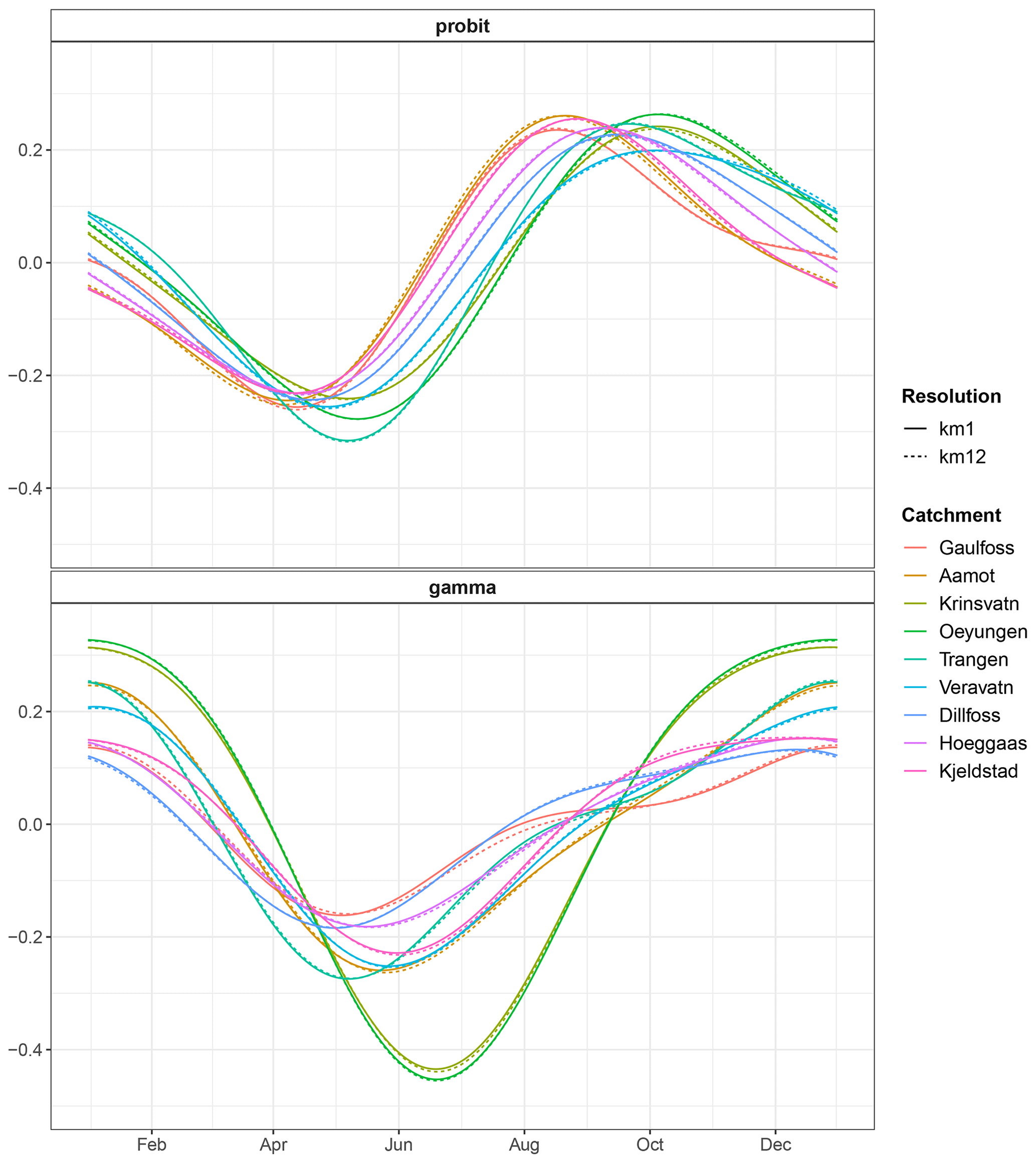
Figure 3 seNorge estimates of the seasonality component in Eq. (7) in the training period 1957–1986 for all catchments at both spatial scales. Top: the estimated seasonality in the mean of the latent Gaussian field μ_st estimated by probit regression. Bottom: the estimated seasonality in the mean of the gamma distribution log (kθ_st) estimated within a GLM/GAM framework.

The models outlined in Sects. 3.1 and 3.2 are fitted to the finer seNorge scale data only for the training period. In order to obtain model parameter estimates at the finer scale in the test period, we need to relate the models at the two scales so that model changes between the training and test periods at the coarser scale can be used to infer model changes at the finer scale. Specifically, we may update the mean of the latent field μ_st in Eq. (1), the parameters of the gamma distribution k and θ_st in Eq. (3), and the autocorrelation coefficient ρ_t in Eq. (11), while the structure of the spatial correlation matrix Σ_t in Eq. (10) is assumed constant for the aforementioned reason.

For μ_st and $\log \left({\mathit{\theta }}_{\text{st}}\right)=\log \left(k{\mathit{\theta }}_{\text{st}}\right)-\log \left(k\right)$, we may update each of the terms in Eqs. (4) and (5), respectively. Here, the seasonality Eq. (7) and the potential linear trend component Eq. (8) of μ_st (and similar for log (θ_st)) are adjusted so that the average adjustment over all the time points in the test period ${\stackrel{\mathrm{‾}}{\mathit{\mu }}}_{s\cdot }^{\mathrm{a}}$ fulfils

$${\stackrel{\mathrm{‾}}{\mathit{\mu }}}_{s\cdot }^{\mathrm{a}}={\stackrel{\mathrm{‾}}{\mathit{\mu }}}_{s\cdot }^{\text{tr}}+\left({\stackrel{\mathrm{‾}}{\mathit{\mu }}}_{r\cdot }^{\text{te}}-{\stackrel{\mathrm{‾}}{\mathit{\mu }}}_{r\cdot }^{\text{tr}}\right),$$

where te indicates the test period, tr indicates the training period, and s is a fine-scale grid cell located within a coarse-scale grid cell r.

Table 2 The estimated trend coefficient in Eq. (8) for each catchment based on data from 1957 to 1986 for μ_st in the probit model (left) and log (θ_st) in the gamma model (right). Estimates are given for both 1 km seNorge data and seNorge data upscaled to 12 km resolution.

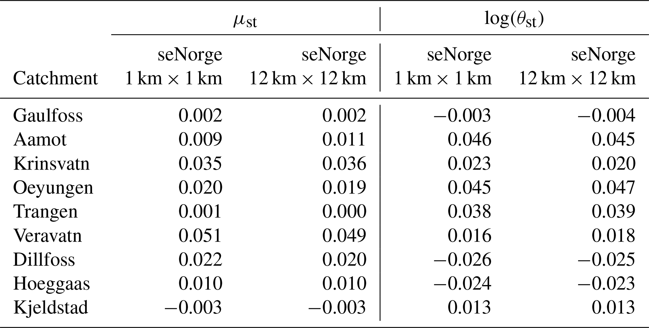
Figure 3 shows the training-period estimates of the seasonality component given in Eq. (7). While the seasonality patterns vary substantially across the different catchments as well as between the two model parts, the estimates are very consistent across the two spatial scales. We thus infer seasonality components for the fine scale during the test period by updating the fine-scale components from the training period according to the estimated changes between the training and test periods at the coarse scale. We see the same patterns for the trend coefficient in Eq. (8); see Table 2. The trend coefficient and the correlation coefficient ρ_t are thus updated in the same manner as the seasonality component. Finally, the shape parameter of the gamma distribution k may be updated so that the ratio of the estimates in the training and test periods at the fine scale equals the ratio of the two estimates at the coarser scale.

In Sect. 4 various versions of the method are compared, where individual model components are either updated according to information based on an RCM output or assumed stationary over the entire time period.

3.4 Daily fine-scale precipitation generator

With the adjustments described above, the marginal models and the space–time Gaussian random field together form a precipitation generator for use on the fine-scale grid in the test period. The parameters of the generator are obtained using seNorge data in the training period and adjusted based on RCM data spanning both the training and test periods. Assume we want to simulate data at all grid-cell locations $s\in \mathit{\{}\mathrm{1},\mathrm{\dots },S\mathit{\}}$ and time points $t\in \mathit{\{}\mathrm{1},\mathrm{\dots },T\mathit{\}}$, a total of S locations and T time points. Data simulation from the generator consists of the following steps, with the superscript a indicating adjusted parameter estimates.

1. For each time point t, spatially correlated but temporally independent random vectors ${\mathit{\eta }}_{\mathrm{t}}^{\ast }$ of size S are drawn from the multivariate Gaussian distribution with mean vector 0 and correlation matrix ${\widehat{\mathbf{\Sigma }}}_{\mathrm{t}}$ specified by the Matérn correlation function, i.e. ${\mathit{\eta }}_{\mathrm{t}}^{\ast }\sim N(\mathbf{0},{\widehat{\mathbf{\Sigma }}}_{\mathrm{t}})$.

2. Temporal correlation is introduced by setting ${\mathit{\epsilon }}_{t+\mathrm{1}}^{\ast }={\widehat{\mathit{\rho }}}_{\mathrm{t}}^{\mathrm{a}}{\mathit{\epsilon }}_t^{\ast }+\sqrt{\mathrm{1}-({\widehat{\mathit{\rho }}}_{\mathrm{t}}^{\mathrm{a}}{)}^{\mathrm{2}}}{\mathit{\eta }}_t^{\ast }$.

3. At grid cell s and time t, the probability of precipitation is ${\widehat{p}}_{\text{st}}^a=\mathrm{\Phi }\left({\widehat{\mathit{\mu }}}_{\text{st}}^{\mathrm{a}}\right)$. The precipitation amount is set as $y_{\text{st}}^{\ast }=\mathrm{0}$ if $\mathrm{\Phi }\left({\mathit{\epsilon }}_{\text{st}}^{\ast }\right)\le \mathrm{1}-{\widehat{p}}_{\text{st}}^a$ and $y_{\text{st}}^{\ast }={\mathrm{\Gamma }}^{-\mathrm{1}}\left(\right(\mathrm{\Phi }\left({\mathit{\epsilon }}_{\text{st}}^{\ast }\right)-(\mathrm{1}-{\widehat{p}}_{\text{st}}^a))/{\widehat{p}}_{\text{st}}^a;{\widehat{k}}^{\mathrm{a}},{\widehat{\mathit{\theta }}}_{\text{st}}^{\mathrm{a}})$ otherwise.

That is, as mentioned above, the fine-scale spatial correlation structure described by ${\widehat{\mathbf{\Sigma }}}_{\mathrm{t}}$ is the single part of the model that is not adjusted based on information from the RCM.

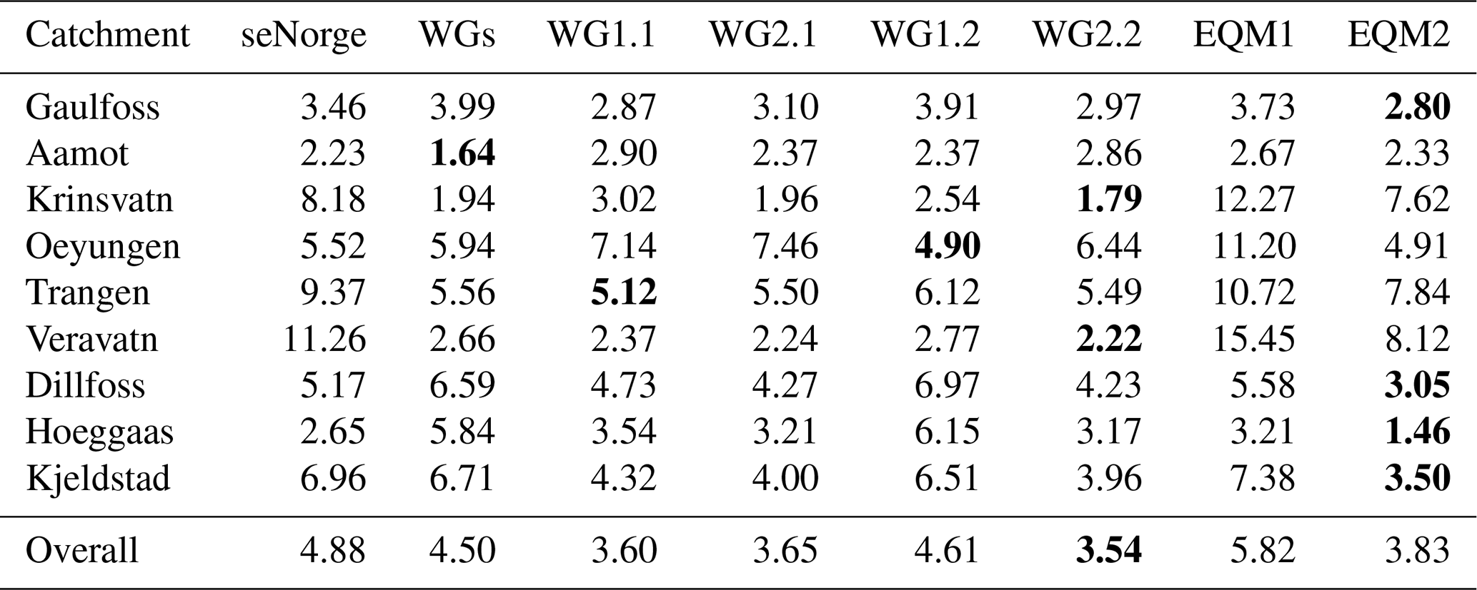
Table 3 Integrated quadratic distance (IQD) values comparing simulated and seNorge distributions over all days in 1987–2005. The results are averaged over all 1 km × 1 km grid cells in each catchment. The simple method seNorge uses the daily values over the period 1957–1986 as a prediction, WGs assumes trends estimated for 1957–1986 continue in 1987–2005, WG1.1 and WG2.1 include seasonality and trend estimates from RCM1 and RCM2, respectively, in the gamma model, while for WG1.2 and WG2.2, RCM information is included in both the gamma model and the probit model. Results of the reference method are denoted EQM1 for RCM1 and EQM2 for RCM2. The best method for each catchment is indicated in bold.

3.5 Reference method

To assess the performance of the proposed method, we use the empirical quantile delta mapping method as a reference. The RCM outputs of approximately 12 km × 12 km resolution are first re-gridded to the 1 km × 1 km seNorge grid using bilinear interpolation, as implemented in the R package akima version 0.6–2 (Akima and Gebhardt, 2016). Wet-day correction is applied prior to bias correction of precipitation amount, as RCM outputs tend to give more rainy days than the observed ones (Frei et al., 2003). Specifically, a threshold value is determined such that the wet-day frequency in the re-gridded RCM dataset is equal to that in the seNorge dataset for the training period; precipitation values below the threshold value are set to zero for both the training and test periods. Correction of precipitation amount in the test period is carried out using the empirical quantile delta mapping method proposed by Cannon et al. (2015), where the relative changes in the precipitation quantiles projected by an RCM from the training period to the test period are explicitly preserved. For individual seNorge grid cells, the method is applied to pooled daily data for each calendar month to ensure an unbiased seasonal cycle and computational efficiency, although this might lead to potential continuity issues at the turn of the month. The method belongs to the class of widely used empirical quantile mapping methods (EQMs), and we will refer to it as such in the following.

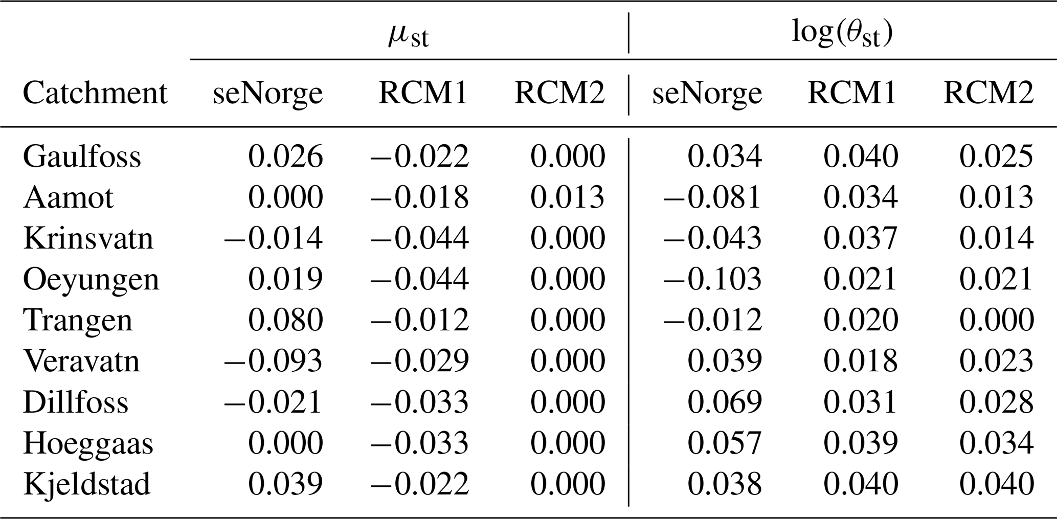
Table 4 Estimated changes in the trend coefficient in Eq. (8) between the training period 1957–1986 and the test period 1987–2005, for μ_st in the probit model (left) and log (θ_st) in the gamma model (right). Estimates for three different data sources at 12 km resolution are shown: upscaled seNorge data and two RCM outputs.

3.6 Evaluation methods

Evaluation and comparison of the different approaches are performed by comparing various aspects of the resulting datasets. For an overall ranking of the approaches, we employ the proper evaluation metric integrated quadratic distance (IQD) that compares the full distributions of observed and modelled precipitation (Thorarinsdottir et al., 2013). That is, denote by F the empirical cumulative distribution function (ECDF) of seNorge precipitation over all time points in the test set at a given grid cell and by G the corresponding ECDF from one of the modelling approaches. The distance between F and G as measured by the IQD is then given by

$$\mathrm{d}(F,G)=\underset{-\mathrm{\infty }}{\overset{+\mathrm{\infty }}{\int }}\left(F\right(x)-G(x){)}^{\mathrm{2}}\mathrm{d}x.$$

The overall performance of the model at a catchment is then calculated as the average IQD over all grid cells in the catchment area, with a lower value indicating a better performance. The IQD fulfils the property that the true data-generating process is expected to obtain an IQD value of 0 when compared against ECDFs based on data samples of any size. It is thus an appropriate metric for ranking competing methods (Gneiting and Raftery, 2007; Thorarinsdottir et al., 2013). For the WG approach, we can easily obtain a precise approximation of the marginal distribution in each grid cell by simulating multiple realizations from each daily distribution. For the EQM approach, however, the marginal distribution in a grid cell is estimated by combining one value for each day in the time period of interest.

For an improved understanding of the behaviour of the models, we further perform several empirical diagnostics. To analyse the marginal distributions at each grid cell, we compare means of daily precipitation, wet-day frequency given by the number of wet days, wet-day intensity as measured by the mean and standard deviation of the precipitation on wet days only, and representation of heavy precipitation as measured by the 95th percentile of positive precipitation. Diagnostics of the temporal data structure are performed by assessing dry–wet temporal patterns and seasonal patterns of temporal autocorrelation coefficients, while empirical functions of Pearson's correlation as a function of distance are used to perform spatial data diagnostics.

4 Results

We perform model inference using data from 1957 to 1986 and infer climate change effects by comparing the coarse-scale RCM data from the two time periods 1957–1986 and 1987–2005. Simulations of fine-scale precipitation for the test set 1987–2005 are then compared against the seNorge data for the test period 1987–2005.

We consider three versions of the WG method, where we include varying degrees of climate change information derived from the RCM data. A stationary version, denoted by WGs, assumes that trends estimated for the seNorge data in the training period continue into the test period, with the remaining model components fixed at their estimates in the training period. That is, no RCM information is used. A version denoted by WG1.1 and WG2.1 for RCM information derived from RCM1 and RCM2, respectively, includes climate change information from the RCM in the seasonality and trend components of the gamma model for precipitation amount on wet days. Finally, a version denoted by WG1.2 and WG2.2 for RCM information derived from RCM1 and RCM2, respectively, includes climate change information from the RCM in the seasonality and trend components of both the gamma model and the probit model for precipitation occurrence. The various WG methods are compared against the reference method in Sect. 3.5 denoted EQM1 and EQM2 derived from RCM1 and RCM2, respectively, as well as a simple method that uses the empirical distributions of the fine-scale seNorge data in the training period directly as predictions for the corresponding empirical distributions of the fine-scale seNorge data in the test period.

4.1 Marginal performance

We evaluate the marginal performance of the simulations by comparing empirical distributions of simulations and observations over all time points in the test set. Specifically, we compare the empirical distribution of the seNorge data in every 1 km × 1 km grid cell to simulations for that same grid cell using the IQD. The average IQD values over all grid cells in each catchments are given in Table 3. Overall, the WG methods that include RCM information perform better than the stationary approach, which again outperforms using the historical data directly. The WG simulations have better performance than the EQM for both RCM1 and RCM2. The best-performing simulation is WG2.2, where both the gamma model for precipitation amount and the probit model for the wet frequency are updated with climate change information from RCM2. The EQM based on RCM2 performs quite well, while the EQM based on RCM1 yields the worst-performing simulations.

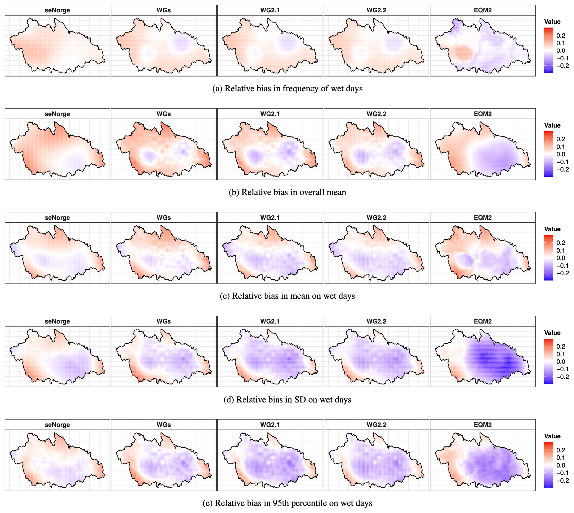
Figure 4 Relative bias in various marginal summary statistics at the 1 km × 1 km scale in the largest catchment, Gaulfoss. The observed seNorge data in the training period 1957–1986, the stationary WGs simulation, and three simulations using climate change information from RCM2 are compared against the seNorge data in the test period 1987–2005.

The IQD values in Table 3 vary substantially across the simulation methods for individual catchments. To investigate this further, we take a closer look at the trend coefficient estimates, as the estimated changes in seasonality are quite stable across catchments for a given RCM and model component (results not shown). The estimates of the trend coefficient in Eq. (8) based on the seNorge training data from 1957 to 1986 are given in Table 2 in Sect. 3.3 above. For the probit model, the trend estimates are positive in all but one catchment, the small inland catchment Kjeldstad, where a small negative trend is estimated. As a result, the probability of precipitation is expected to increase over time. The rate of the increase varies substantially for the different catchments, ranging from 0.001 in Trangen to 0.051 in Veravatn. For the gamma distribution, the trend coefficient estimates are highly varying across catchments, with negative estimates for three catchments and positive estimates for six catchments, indicating no consistent trend pattern in the amount of daily precipitation on wet days. When fitting these models to the RCM data in the training period, we found insignificant trend estimates for the probit model in seven catchments based on RCM1 and five based on RCM2, while the number of cases for the gamma model is six based on RCM1 and four based on RCM2.

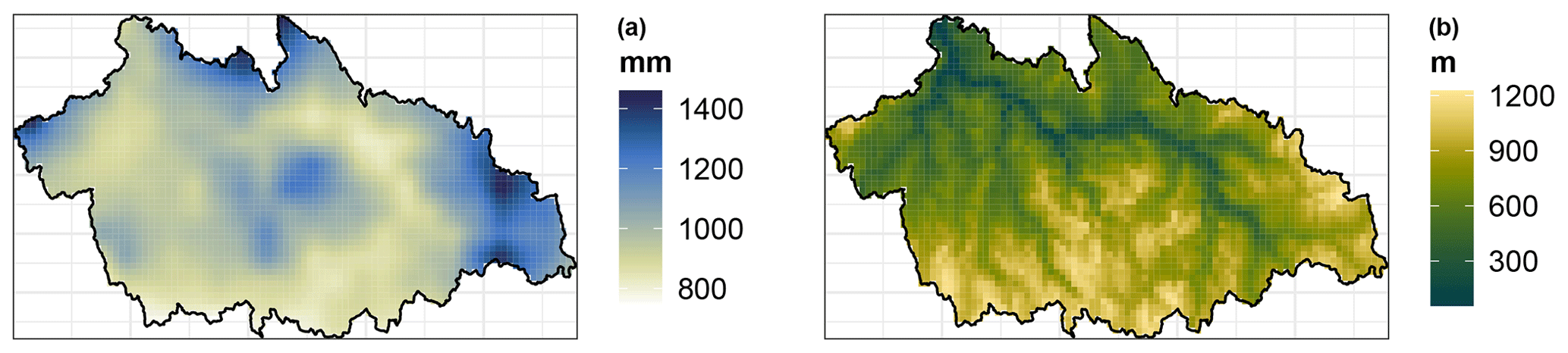
Figure 5 Average annual precipitation (a) in the period 1957–2005 and the digital elevation map (b), both at the 1 km × 1 km scale in the catchment Gaulfoss.

Figure 6 Empirical spatial correlation of precipitation amount at the catchment Gaulfoss for each month of the year. Results are shown for the seNorge data in the test period 1987–2005 (red dots) and for the EQM simulation based on RCM2 (cyan dots). The Matérn spatial correlation estimated with the WG method based on seNorge data in the training period 1957–1986 is indicated in grey, with the width of the bar indicating the spread of the daily estimates within the month.

The estimated changes in trend coefficients at the 12 km × 12 km scale between the training and test periods are listed in Table 4. The zeros in the table indicate that the changes are not significantly different from 0 at the 0.05 level. The seNorge estimates for the probit model are mostly positive, corresponding to a higher trend estimate in the test period than the training period. The estimates based on RCM1 are consistently negative, while no change is estimated based on RCM2 except for Aamot. For the gamma model, approximately as many positive and negative values are observed, while estimates in all catchments are positive by both RCMs. Note that the stationary simulation WGs assumes the same trends in the training and test periods, corresponding to values of 0 in Table 4.

The simulations WGs, WG1.1, and WG2.1 share the same probit model for precipitation occurrence, while the gamma model for the precipitation amount differs. For the gamma model, five catchments have a strong positive climate change signal according to the upscaled seNorge data, where both RCMs project a change in the same direction. Looking at the IQD values in Table 3, we see this translates directly into lower IQD values compared to the WGs simulations. IQD values are higher than WGs in the three catchments closest to the coast (Aamot, Krinsvatn, and Oeyungen), where both RCMs project a positive change against the observed negative change. For Trangen, WG2.1 and WGs have similar IQD values because they both apply no change in the trend. In general, both RCMs provide useful climate change information for the gamma model, which makes the overall performance of WG1.1 and WG2.1 better than WGs.

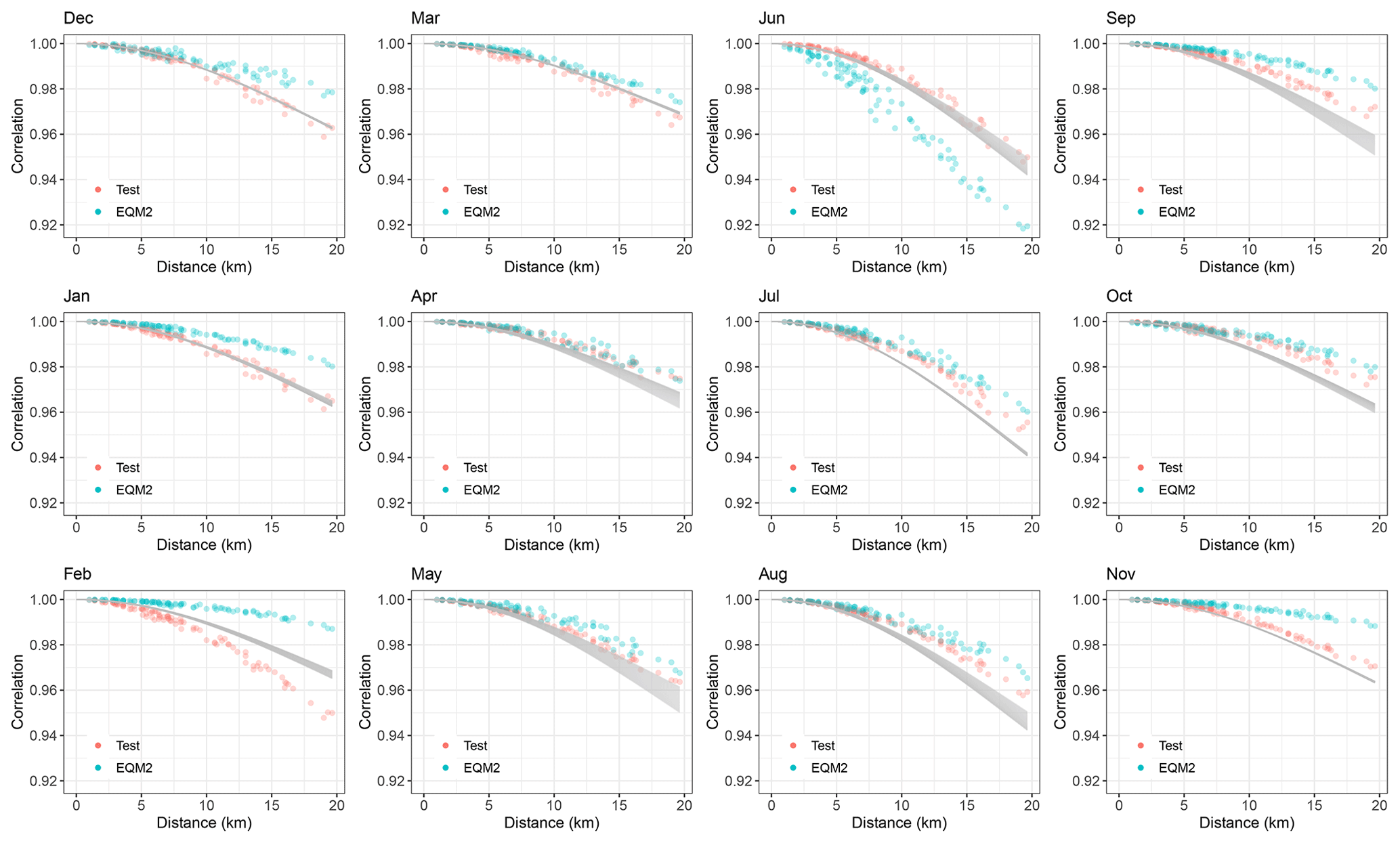
Figure 7 Empirical spatial correlation of precipitation amount at the catchment Kjeldstad for each month of the year. Results are shown for the seNorge data in the test period 1987–2005 (red dots) and for the EQM simulation based on RCM2 (cyan dots). The Matérn spatial correlation estimated with the WG method based on seNorge data in the training period 1957–1986 is indicated in grey, with the width of the bar indicating the spread of the daily estimates within the month.

A similar effect can be seen when comparing the IQD values for Gaulfoss, Trangen, and Kjeldstad based on the simulations WG1.1 and WG1.2. While these two simulations share the same gamma model, WG1.1 assumes a stationary probit model and WG1.2 applies climate change information from RCM1 to the precipitation occurrence. Here, the climate change estimates from RCM1 are negative, going in the opposite direction to the seNorge data, and accordingly WG1.2 is worse than WG1.1, which assumes no change in the trend. The negative change applied in WG1.2 in Hoeggaas can also relate to the reduced performance compared with WG1.1. In Veravatn and Dillfoss, however, the estimates based on RCM1 are in the same direction as the observed ones, but this somehow does not translate into a better performance of WG1.2. For Aamot, where no change is estimated by the seNorge data, a negative change by RCM1 seems to make WG1.2 better than WG1.1, and a positive change by RCM2 makes it the only catchment where WG2.2 is worse than WG2.1. In the other catchments, WG2.2 is slightly better than WG2.1 given that they both apply no change in the trend of the probit model; this indicates that the changes in the seasonality projected by RCM2 are generally reasonable, and only the effect seems limited in most catchments.

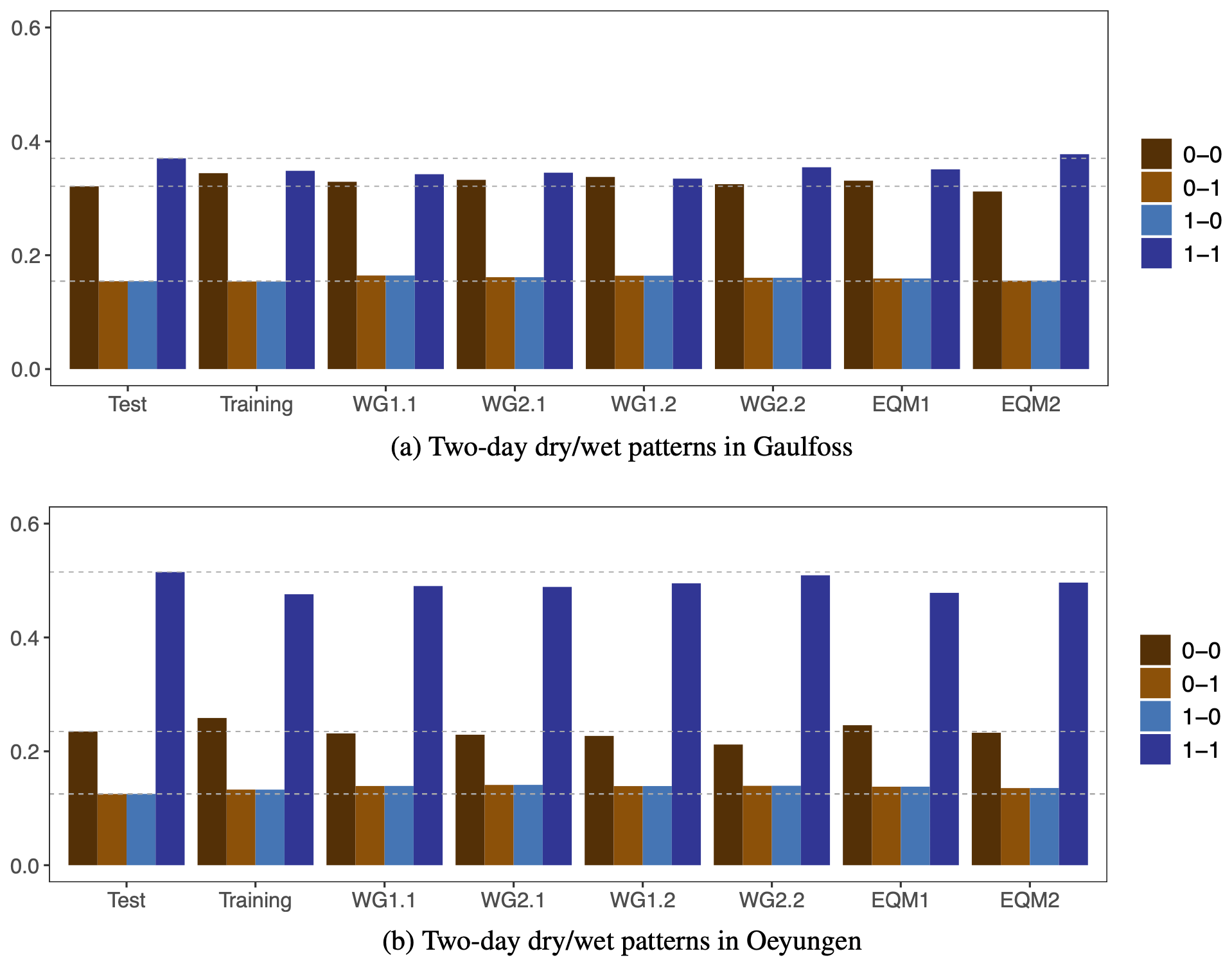
Figure 8 Proportion of different 2 d dry–wet patterns for the seNorge data in the training period 1957–1986 and the test period 1987–2005 as well as for six different simulations of the test period. The results are aggregated over all grid cells in the catchments Gaulfoss (a) and Oeyungen (b). Dry days are indicated with 0 and wet days with 1. For ease of interpretation, horizontal dashed lines are drawn at the levels of the test set.

Further analysis of the marginal performance of four of the simulations as well as the seNorge reference is shown in Fig. 4 for the largest catchment, Gaulfoss, while the climatology and elevation information is given in Fig. 5. The leftmost plot in Fig. 4a shows that the frequency of wet days for the seNorge data is generally lower in the training period than the test period. This again results in a significant bias in the overall mean (see Fig. 4b), while the general correspondence between the amount distributions on wet days is quite good. Here, the IQD value is 3.46 for seNorge, 3.99 for WGs, 3.10 for WG2.1, 2.97 for WG2.2, and 2.8 for EQM2. WG2.1 and WG2.2 share the same distribution for the precipitation amount on wet days, and given that RCM2 projects zero change in the trend of the probit model, performance of the two simulations is different solely due to the different seasonality, which again is minimal; see Fig. 4a. While EQM2 has the lowest IQD value, it appears that this method overestimates the wet frequency (see Fig. 4a), the spread on wet days (Fig. 4d), and thus also the 95th percentile on wet days (Fig. 4e). However, the IQD score is less sensitive to these errors than to the erroneous overall mean.

Figure 9 Smoothly changing daily estimates of the correlation coefficient ρ_t in Eq. (11) for each catchment, estimated based on the seNorge data in the training period 1957–1986 (green dotted lines), inferred by adding the climate change information from RCM1 (cyan dashed lines) and RCM2 (purple dashed lines) for the test period 1987–2005, and as a reference the values estimated based on the seNorge data in the test period 1987–2005 (red solid lines).

4.2 Spatial and temporal correlation structure

The spatial correlation structure at the 1 km × 1 km scale cannot be inferred from the 12 km × 12 km RCM data, and we thus assume that the fine-scale spatial correlation estimated based on the training data also holds for the test data. This is assessed in Fig. 6 for the largest catchment, Gaulfoss, and in Fig. 7 for the smallest catchment, Kjeldstad. The Matérn correlation function estimated based on the training data appears to capture the overall structure of the test data, indicating no large deviations in spatial structure between the two time periods. However, there are some smaller deviations, indicating smaller changes in the seasonal pattern of the spatial structure. In particular, the estimated correlation is slightly higher than that observed in February and somewhat lower in autumn, especially at Kjeldstad. For both catchments, the largest spread of the daily estimates of the correlation function is in the spring months of April and May.

The spatial structure of the EQM simulation differs somewhat from that of the data. The correlation is too strong in the winter months of December, January, and February and too weak in June. It further appears that the EQM is more successful in modelling the spatial correlation of the data from the larger catchment Gaulfoss than the data from the small catchment Kjeldstad, whose area of 144 km² is approximately 5 % of the area of Gaulfoss at 3084 km².

In order to assess the temporal correlation structure of the various simulations, first consider the 2 d dry–wet patterns shown in Fig. 8. For the inland catchment Gaulfoss, the proportions of 2 consecutive dry days and 2 consecutive wet days is approximately equal in the training set, while the test set has fewer instances of 2 consecutive dry days, with a corresponding increase in 2 consecutive wet days. The proportions of 2 consecutive dry or wet days for the simulations are mostly in between the values for the seNorge training and test sets, except for EQM2, which has the highest frequency of wet days; see also Fig. 4a. At the coastal catchment Oeyungen, nearly 50 % of all the 2 d patterns observed in the training period, and over 50 % in the test set, are 2 consecutive wet days. Here, all the simulations yield a lower proportion of 2 consecutive wet days than the observed test data, while the proportions of pairs with 1 wet day and 1 dry day is higher. The results shown here for the WG method are based on a single simulation for each model version. We found that these results may vary slightly between realizations from the same model (results not shown). In addition, we have compared the sequencing of dry days generated by different methods and found that the distribution of dry spells is similar across all simulations for a given catchment, where the majority consist of the short-term cases and a drought event longer than 2 weeks is rare (results not shown).

The temporal correlation applied in the daily fine-scale precipitation generator for the test period is assessed in Fig. 9. As described in Sect. 3.2, the short-term autocorrelation of the WG model is introduced through the temporal dependence in the underlying spatial random field. Data at both spatial scales have the same temporal dimensionality, and we thus assume that the fine-scale temporal correlation coefficients ρ_t can be updated by the changes projected by an RCM between the training and test periods. Estimates based on seNorge data in the training period indicate higher temporal dependence in spring and winter and lower dependence in summer. In the test period, dependence becomes lower in spring and summer and higher in October and November. The changes in spring are generally not realistically projected by RCMs, except for RCM2 in Trangen, while the changes in summer and early winter are better captured by RCM2 than RCM1 in most catchments.

5 Conclusions and discussion

This paper proposes a two-step stochastic downscaling and bias-correction approach for future projection of daily precipitation. In a first step, a stochastic weather generator for a high-resolution grid is developed using a historical gridded observation-based data product. In a second step, the weather generator is inferred for a future climate by using only the projected changes between a historical reference period and a future period based on a coarser-scale RCM. In the current application, the observation-based data product is available on a 1 km × 1 km grid, and the climate change information stems from an RCM on a 12 km × 12 km grid. In this setting, there appears to be good correspondence between catchment-scale seasonality and linear trend patterns at the two spatial resolutions, making the transformation of information between the two scales feasible.

The WG approach is applied to data from nine hydrological catchments in central Norway, with each study area ranging in size from approximately 1000 to 5500 km² and compared against an EQM and a simple persistence reference method. The methods are trained on daily data from 1957 to 1986 and tested on out-of-sample data from 1987 to 2005. Based on an evaluation of the resulting marginal distributions, the WG method overall outperforms the EQM approach, both in terms of the IQD score and based on empirical assessment of marginal summary statistics. However, all the simulation methods show large variations in the performance between individual catchments. The WG method furthermore yields realistic temporal and spatial correlation structures.

The historical RCM runs used here are available until 2005, and the observation-based data are available from 1957, yielding a dataset with 49 years of data. With 30 years of data used to train the models, this leaves only 19 years of data for the out-of-sample evaluation. With only 19 years of data in the test period, we may expect to see some effects of natural variability when comparing the seNorge data product and the largely free-running RCMs. Looking at the linear trend coefficient in the probit model, it seems that the seNorge data upscaled to 12 km resolution are generally able to capture the change where there are proportionally more wet days in the test period than in the training period, while the RCM data either project strong negative changes or simply no change in most catchments. For the gamma model, however, both RCMs seem to have projected correct changes in the trend and seasonality. Overall, we see that all versions of the WG method yield better performance than the marginal persistence reference method based on seNorge data from 1957 to 1986, and including RCM information improves upon the stationary WG approach. Furthermore, the transparent way in which the RCM information is included in the WG simulations allows for a direct assessment of this information and its plausibility (Maraun et al., 2017).

In our case study, the training and test periods are two consecutive time periods. However, in climate change impact studies, there is commonly a large gap of the order of decades between the historical period and the future period of interest. In this case, it may be necessary to expand our proposed model to also account for large-scale climate oscillation or teleconnection patterns, such as the El Niño–Southern Oscillation (ENSO) and the Indian Ocean Dipole (IOD), particularly in regions where rainfall climatologies are dominated by such patterns (e.g. Wu et al., 2003; Andreoli and Kayano, 2005). In such cases, specific components of the model, e.g. the spatial correlation structure, may need to be estimated depending on both seasonal variation and oscillation modes. To assess this, the parameter estimation procedure can be extended to obtain separate estimates for both months and oscillation modes. The series of parameter estimates can then be assessed for seasonal and oscillation dependence using standard regression techniques.

While the application in this paper focuses on climate projections, the modelling framework proposed here provides a more general approach to computationally efficient stochastic downscaling of precipitation. Other potential applications include seasonal and decadal weather and climate predictions. The availability of computationally efficient downscaling methods is especially important in settings where large ensembles are needed in order to achieve prediction skill; see e.g. Smith et al. (2019).