the Creative Commons Attribution 4.0 License.
the Creative Commons Attribution 4.0 License.
 | 24 Sep 2021
Relative humidity gradients as a key constraint on terrestrial water and energy fluxes
Monica Garcia
Laura Morillas
Ulrich Weber
T. Andrew Black
Mark S. Johnson
Earth's climate and water cycle are highly dependent on terrestrial evapotranspiration and the associated flux of latent heat. Although it has been hypothesized for over 50 years that land dryness becomes embedded in atmospheric conditions through evaporation, underlying physical mechanisms for this land–atmosphere coupling remain elusive. Here, we use a novel physically based evaporation model to demonstrate that near-surface atmospheric relative humidity (RH) fundamentally coevolves with RH at the land surface. The new model expresses the latent heat flux as a combination of thermodynamic processes in the atmospheric surface layer. Our approach is similar to the Penman–Monteith equation but uses only routinely measured abiotic variables, avoiding the need to parameterize surface resistance. We applied our new model to 212 in situ eddy covariance sites around the globe and to the FLUXCOM global-scale evaporation product to partition observed evaporation into diabatic vs. adiabatic thermodynamic processes. Vertical RH gradients were widely observed to be near zero on daily to yearly timescales for local as well as global scales, implying an emergent land–atmosphere equilibrium. This equilibrium allows for accurate evaporation estimates using only the atmospheric state and radiative energy, regardless of land surface conditions and vegetation controls. Our results also demonstrate that the latent heat portion of available energy (i.e., evaporative fraction) at local scales is mainly controlled by the vertical RH gradient. By demonstrating how land surface conditions become encoded in the atmospheric state, this study will improve our fundamental understanding of Earth's climate and the terrestrial water cycle.
- Article
(5027 KB) - Full-text XML
-
Supplement
(845 KB) - BibTeX
- EndNote


Latent heat flux (LE) associated with plant transpiration and evaporation from soil and intercepted water (i.e., evapotranspiration, ET) links the water cycle with the terrestrial energy budget. More than half of the incoming radiation energy at the land surface is consumed as LE, making ET the second largest flux in the terrestrial water balance after precipitation (Oki and Kanae, 2006). Also, LE is a controlling factor for near-surface climatic conditions such as temperature and humidity (Ma et al., 2018; Byrne and O'Gorman, 2016). While most research has been devoted to developing and improving rate-limiting parameters constraining LE (e.g., García et al., 2013; Martens et al., 2017), exploring the governing physics of LE has received less attention following earlier pioneering work (Schmidt, 1915; Penman, 1948; Bouchet, 1963; Monteith, 1965; Priestley and Taylor, 1972). Nevertheless, improvement of the theoretical understanding of LE still remains an essential cornerstone to correctly simulate and predict climate and hydrological cycles (Emanuel, 2020).
Climatic conditions over the land surface have been getting not only warmer but also drier in recent decades (i.e., decrease in relative humidity) (Sherwood and Fu, 2014; Willett et al., 2014; Byrne and O'Gorman, 2018), but land–atmosphere feedback processes shaping the near-surface atmospheric state are still not well understood. In the early 1960s, Bouchet (1963) hypothesized that land surface dryness is coupled to the atmospheric state through LE, with the Bouchet hypothesis now widely accepted (Ramírez et al., 2005; Fisher et al., 2008; Mallick et al., 2014). However, the underlying physical mechanisms for this land–atmosphere coupling still remain elusive (McNaughton and Spriggs, 1989). Recently, McColl et al. (2019) introduced a novel theoretical perspective on land–atmosphere coupling which is referred to as “surface flux equilibrium (SFE)”. They hypothesized that relative humidity (RH) reaches a steady-state value in an idealized atmospheric boundary layer at daily to monthly timescales. Under steady RH conditions (i.e., the SFE state), LE can be determined using only the atmospheric state and radiative energy. Although this method performed well compared to actual LE observations for inland continental sites (McColl and Rigden, 2020; Chen et al., 2021), a further investigation is needed to understand how dynamics of turbulent heat fluxes in the atmospheric surface layer at sub-daily timescales evolve to the SFE state.
A traditional way to express the atmospheric surface layer processes is to partition LE into diabatic and adiabatic processes using the Penman–Monteith (PM) equation (Monteith, 1965), as proposed by Monteith (1981). The PM equation combines the energy balance equation with mass-transfer theory for water vapour and sensible heat, resulting in diabatic (radiative energy-related) and adiabatic (vapour pressure deficit-related) processes for a parcel of air in contact with a saturated surface (Monteith, 1981).
where S is the linearized slope of saturation vapour pressure versus temperature (hPa K−1), γ is the psychrometric constant (hPa K−1), ρ is the air density (kg m−3), cp is the specific heat capacity of air at constant pressure (MJ kg−1 K−1), and Q is available radiative energy (i.e., the difference between net radiation (Rn) and soil heat flux (G) expressed in units of W m−2). e∗(Ta) is the saturation vapour pressure (hPa) corresponding to the air temperature (Ta) measured at a reference height (typically 2 m or eddy flux measurement height), and ea is vapour pressure (hPa) at the reference height. is known as atmospheric vapour pressure deficit (VPD, expressed in units of hPa). ra is aerodynamic resistance to heat and water vapour transfer (s m−1), and rs is surface resistance to water vapour transfer (s m−1) representing drying soil and/or plant stomatal closure.
In principle, high Q and VPD at the reference height increase the diabatic and the adiabatic terms respectively in the PM equation, and as such, Q and VPD are the two primary drivers of evaporation (Monteith and Unsworth, 2013). Yet, this “high VPD leads to high LE” interpretation cannot be generalized because rs increases with VPD due to stomatal closure by vegetation under high-VPD conditions (Tan et al., 1978; Novick et al., 2016; Massmann et al., 2019). While the PM equation is useful to explore biological control of LE through rs (Jarvis and McNaughton, 1986; Peng et al., 2019), physical mechanisms corresponding to each term in Eq. (1) are less intuitive due to the sensitivity of rs to VPD. As a result, how the atmospheric state affects evaporation and vice versa remains ambiguous in the PM equation.
Is there a way to mathematically express the physical mechanisms of LE without requiring rs? In this paper, we present a pair of equations expressing actual LE as a combination of diabatic and adiabatic processes without requiring rs. Similar to the PM equation, our new equations are derived by combining the energy balance equation with the flux gradient equations, but crucially ours do not include rs. The novel equations are applied empirically to eddy-covariance observation sites and a global LE dataset to explore land–atmosphere coupling processes at various spatiotemporal scales. To do this, we decomposed observed LE into adiabatic and diabatic components and discuss how these patterns can help to understand land–atmosphere interactions and potential responses under future climatic conditions.
2.1 A pair of evaporation equations for an unsaturated surface
In this section, we derive a pair of evaporation equations for an unsaturated surface. In this derivation, we assume a horizontally homogenous landscape where the sources of water vapour and heat are identical. Under this idealized condition, aerodynamic resistances (ra) to heat and water vapour transfers are identical. Here, ra is a parameterization of turbulent mixing due to mechanical turbulence and buoyancy driven by surface heating.
We first express LE using a flux gradient equation as , where es is the surface vapour pressure. Here, the subscript s indicates the land surface which is defined as an idealized plane specified as the sum of displacement height and roughness length for heat (Knauer et al., 2018a; Novick and Katul, 2020). If the land surface is saturated, es becomes equivalent to the saturation vapour pressure (i.e., ). For an unsaturated land surface, however, relative humidity should be introduced as , where RHs is surface relative humidity, i.e., the ratio of es to e∗(Ts). For a vegetated surface, RHs as defined in this study represents relative humidity of the foliage surface and is conceptually equivalent to surface water availability in Li and Wang (2019). For a bare soil land surface, RHs represents soil surface relative humidity, which can be found using the “alpha” method that is parameterized using soil moisture content or soil water potential (Lee and Pielke, 1992; Wu et al., 2000; Cuxart and Boone, 2020). Using RHs, LE can be written as for an unsaturated surface condition.
In order to decompose LE into two individual fluxes related to temperature and relative humidity gradients, we add (or ) to the numerator of the flux gradient equation and rewrite LE as follows.
We then approximate using the saturation vapour pressure slope at the air temperature (S), and we introduce a flux gradient equation for sensible heat flux (i.e., ) into Eqs. (2) and (3). Then, the energy balance equation is combined to substitute H with Q−LE. As results, LE can be expressed as follows:
where LEQ (and LE) is a diabatic component, and LEG (and LE) is an adiabatic component of latent heat flux. While the diabatic component is mainly determined by available energy (Q), the adiabatic component is driven by turbulent mixing and vertical gradient of RH. Monteith (1981) originally suggested an equation equivalent to Eq. (4) for the case when the surface does not reach saturation. To our knowledge, Eq. (5) is derived for the first time here. Equations (4) and (5) include RHs to compensate for eliminating rs from the original PM equation.
Since the adiabatic processes in Eqs. (4) and (5) are controlled by the vertical difference of RH, we refer to Eqs. (4) and (5) as the proposed PMRH model (Penman–Monteith equation expressed using RH) to distinguish it from the original PM model. The two Eqs. (4) and (5) are complementary to each other in that they represent distinct thermodynamic paths, each of which will be discussed in the next section. Arguably, applying PMRH can provide new insights into the fundamental mechanisms of LE, particularly when it is decomposed into its diabatic component (LEQ or LE) and its adiabatic component (LEG or LE). In the following sections, we will discuss theoretical meanings of Eqs. (4) and (5) in depth.
2.2 Generalized Penman equation
Before discussing PMRH in depth, we revisit the Penman equation (Penman, 1948) to help with the physical reasoning behind our proposed framework. The widely recognized form of the Penman equation, which was developed as an LE model for a saturated surface, is as follows:
We rearrange this formulation to derive Eq. (7) by factoring out e∗(Ta) and introducing into the second term.
Equations (6) and (7) are mathematically equivalent, but their interpretations are quite different. In Eq. (6), the adiabatic process is controlled by VPD at the reference height. However, in Eq. (7), the adiabatic process acts over the vertical RH gradient, i.e., the difference in RH from the surface to the reference height (RHa). Since the Penman equation is a model for saturated surfaces, 1−RHa in Eq. (7) indicates the difference in RH over the vertical distance between the ground surface and the reference height. Arguably, Eq. (7) is more thermodynamically sound compared to Eq. (6) since RH is an ideal-gas approximation to the water activity (Lovell-Smith et al., 2015) which represents the chemical potential of water (μw) (Monteith and Unsworth, 2013; Kleidon and Schymanski, 2008). When the vertical gradient of RH dissipates owing to well-developed turbulence, the land surface and the atmosphere are in thermodynamic equilibrium (Kleidon et al., 2009). Therefore, taking Eq. (7) instead of Eq. (6) allows us to view the adiabatic process of the Penman model as an equilibration process driving land–atmosphere equilibrium by bringing the surface μw to that of the atmosphere.
As with our interpretation of the Penman model, we can view Eqs. (4) and (5) as a generalized form of the Penman model. Here, the LEG (or LE) term is an equilibration process between the land and the atmosphere when the land surface is not saturated. It is worth noting that LEG can be negative when RHs is less than RHa. Thus, the LEG term operated by turbulent mixing acts to reduce the vertical RH gradient. This physical interpretation is consistent with recent findings that the variance of the RH gradient tends to be minimized over the course of the day, implying that the difference between RHs and RHa is reduced (Salvucci and Gentine, 2013; Rigden and Salvucci, 2015). The diabatic LEQ (or LE) term can be understood as equilibrium LE for an unsaturated surface, which we discuss later in Sect. 2.4.
2.3 Thermodynamic paths
How can we interpret the two formulas of PMRH in Eqs. (4) and (5)? To explain the two forms, the psychrometric relationship is applied to a parcel of air near an unsaturated land surface that is under constant pressure and steadily receiving radiation energy. The psychrometric diagram in Fig. 1 describes the magnitude of turbulent flux (where the length of the arrow corresponds to the magnitude) from the view point of a parcel of air located at a reference height (an approach based on work by Monteith, 1981). Since the parcel of air receives heat and water vapour from the land surface, the final state is represented by the surface condition, while the initial state is represented by the atmospheric conditions at the reference height. Therefore, the initial thermodynamic state of the air parcel can be represented by its temperature and water vapour pressure such as point A in Fig. 1. The initial state is changed by two processes as follows: (1) equilibrating between the land surface (RHs) and the air parcel (RHa) and (2) increasing enthalpy forced by the incoming energy. It should be noted that the changing process (i.e., thermodynamic path) from the initial to the final states in this discussion should be understood as the magnitude of the turbulent heat fluxes.
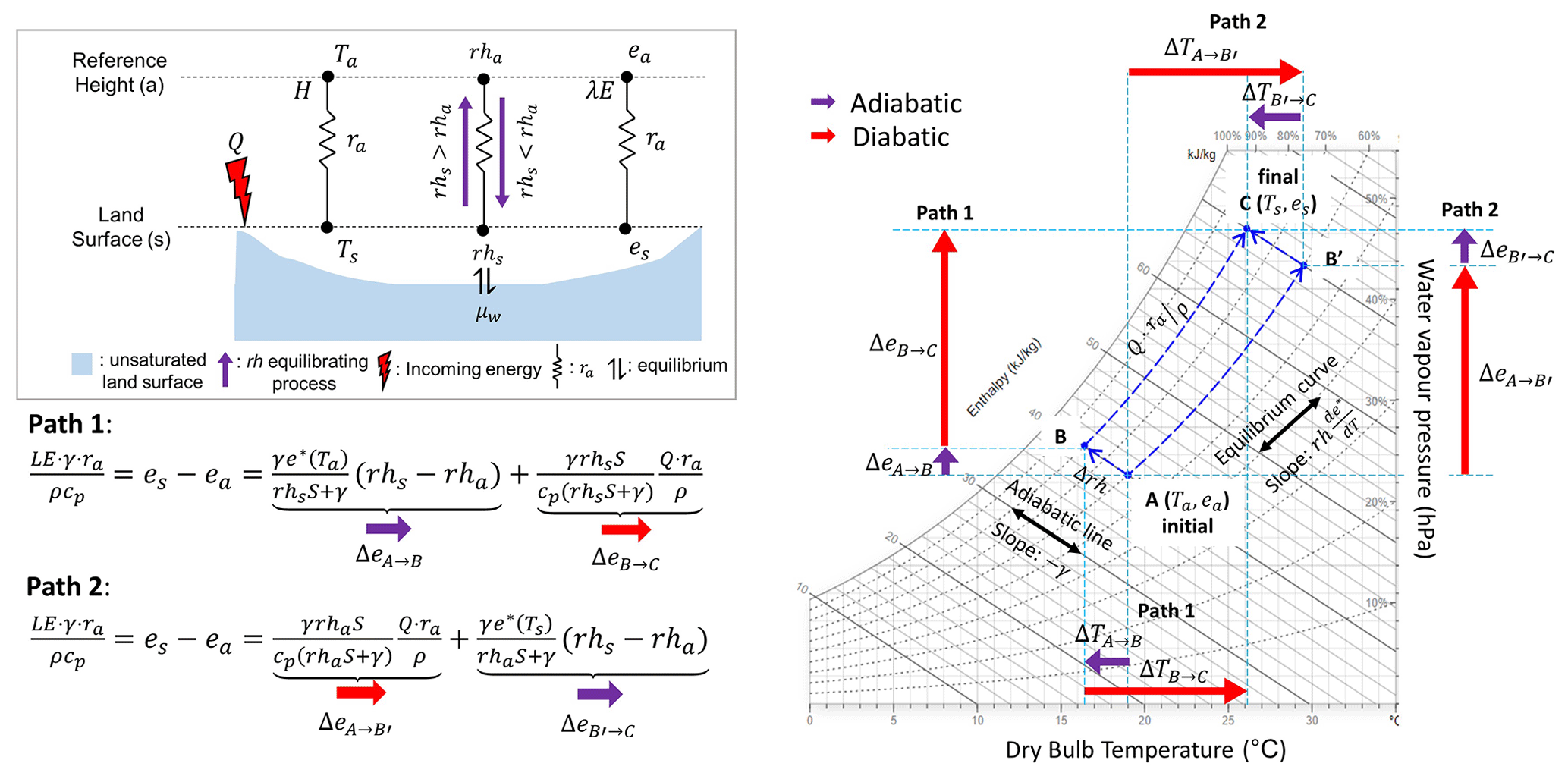
Figure 1Schematic conceptualization of the PMRH model and psychrometric relationship of PMRH. The example psychrometric chart is modified from Marsh (2018). Path 1 represents Eq. (4) divided by while Path 2 represents Eq. (5) divided by . Here, the enthalpy change of the air parcel is defined as (kJ kg−1). It should be noted that the difference between the initial and the final states represents the magnitude of the turbulent heat fluxes instead of changes in atmospheric state.
In the RH equilibrating process, the air parcel is adiabatically cooled (or heated when RHs < RHa) due to turbulent mixing, while the enthalpy of the parcel is not changed. Therefore, the increase (decrease) in latent heat content in the parcel is exactly balanced by a decrease (increase) in sensible heat (A→B in Fig. 1: trajectory along constant enthalpy line). This process is equivalent to the LEG term in Eq. (4). Now, the air parcel is in thermodynamic equilibrium with the land surface (point B in Fig. 1). Then, the air parcel receives energy while the equilibrium is sustained (i.e., RHs is steady), which increases both the temperature and absolute water vapour content of the air parcel (B→C in Fig. 1). This process can be expressed as LEQ of Eq. (4). Consequently, the thermodynamic state of the air parcel approaches point C in Fig. 1.
However, we should recognize that temperature and vapour pressure are “state” variables, meaning that they do not depend on the thermodynamic path by which the system arrived at its final state (Iribarne and Godson, 1981). In the above example, we conceptually followed the adiabatic process first and then the diabatic process (Path 1 in Fig. 1), but one can imagine the opposite order. If we choose Path 2 in Fig. 1, the diabatic process comes first, and thus RHa instead of RHs is preserved while enthalpy increases (i.e., LE), and the adiabatic process is followed at temperature of TS (i.e., LE). Path 2 is described by Eq. (5).
Therefore, one can interpret the two forms of PMRH in Eqs. (4) and (5) as two thermodynamic paths where the diabatic and adiabatic processes occur simultaneously. It should be noted that the diabatic and adiabatic processes in PMRH are “path” functions and thus they vary by path. For instance, LEQ is slightly higher than LE when RHs > RHa. Also, the absolute magnitude of LE is always bigger than that of LEG when Q>0 (i.e., vector is longer than vector A→B in Fig. 1).
2.4 Equilibrium LE for an unsaturated surface
Another distinct characteristic of the PMRH model is the way it defines equilibrium at the land–atmosphere interface. Unlike many previous studies which focused on the steady state of VPD (McNaughton and Jarvis, 1983; Priestley and Taylor, 1972; Raupach, 2001), land–atmosphere equilibrium is achieved in the PMRH model when the vertical RH gradient (i.e., the μw gradient) dissipates. That is, if RHs≈RHa, then it follows that LEG (or LE) is zero and thus LE becomes
We note that Eq. (8) is identical to the SFE theory recently introduced by McColl et al. (2019). They hypothesized that in many continental regions, the near-surface atmosphere is in a state of equilibrium, where RH is steady with time in an idealized atmospheric boundary layer at longer than daily timescales. Equation (8) successfully predicted observed LE at daily and monthly timescales for inland regions (McColl and Rigden, 2020; Chen et al., 2021), which implies the vertical RH gradient tends to evolve toward zero at longer timescales than the sub-daily scale. This is logical in that LEG itself diminishes the vertical RH gradient over the course of a day.
From a different standpoint, if an observed LE is bigger or smaller than Eq. (8) at a longer timescale such as monthly, it may indicate that the land surface conditions are not completely embedded in the near-surface atmospheric state due to highly wet or dry land conditions. Therefore, LEG (or LE) value and sign at monthly timescales could be a useful indicator reflecting land surface dryness relative to the atmosphere.
When both land surface and atmosphere are saturated (i.e., ), Eq. (8) becomes classical equilibrium LE (i.e., ). This is consistent with one of the classical definitions of equilibrium LE that defines equilibrium LE as evaporation from a saturated surface into saturated air (Schmidt, 1915; Eichinger et al., 1996; Raupach, 2001; McColl, 2020). Therefore, we can regard Eq. (8) as a generalized equilibrium LE for an unsaturated surface.
In the following sections, we present a novel physical decomposition of LE from PMRH into LEQ and LEG components to aid in understanding the governing physics of LE. Also, the proportion of net available energy consumed in evapotranspiration, known as the evaporative fraction (EF) is decomposed into and . We conducted a detailed diagnostic analysis of the PMRH model using the multi-year record of an eddy covariance (EC) flux observation site located in a wet–dry tropical climate. We also applied the PMRH model to the 212 EC sites represented in the FLUXNET2015 dataset (Pastorello et al., 2020) and to the FLUXCOM global LE product (Jung et al., 2019). We describe the local and global datasets and analysis methods here before presenting the results.
3.1 In situ EC flux observation
In situ half-hourly EC observations used in this study were made from 2015 to 2018 on a ratoon sugarcane farm in the province of Guanacaste, Costa Rica (10∘25′07.60′′ N, 85∘28′22.22′′ W). The site has a wet–dry tropical climate with a dry season from December to March and a median monthly air temperature ranging from 27 to 30 ∘C. The study site experienced a significant drought in 2015 as the lowest precipitation rate in Fig. 2b (Hund et al., 2018; Morillas et al., 2019). The site was irrigated occasionally during dry seasons via furrow irrigation events, except for 2016 when there was no irrigation due to crop replanting. Due to the ratooning practice (i.e., sugarcane cutting each year followed by resprouting without replanting, detailed explanation in the Supplement), the sugarcane growing seasons varied by year, which provided an opportunity to explore distinct and varied combinations of land surface vs. atmospheric aridity conditions.
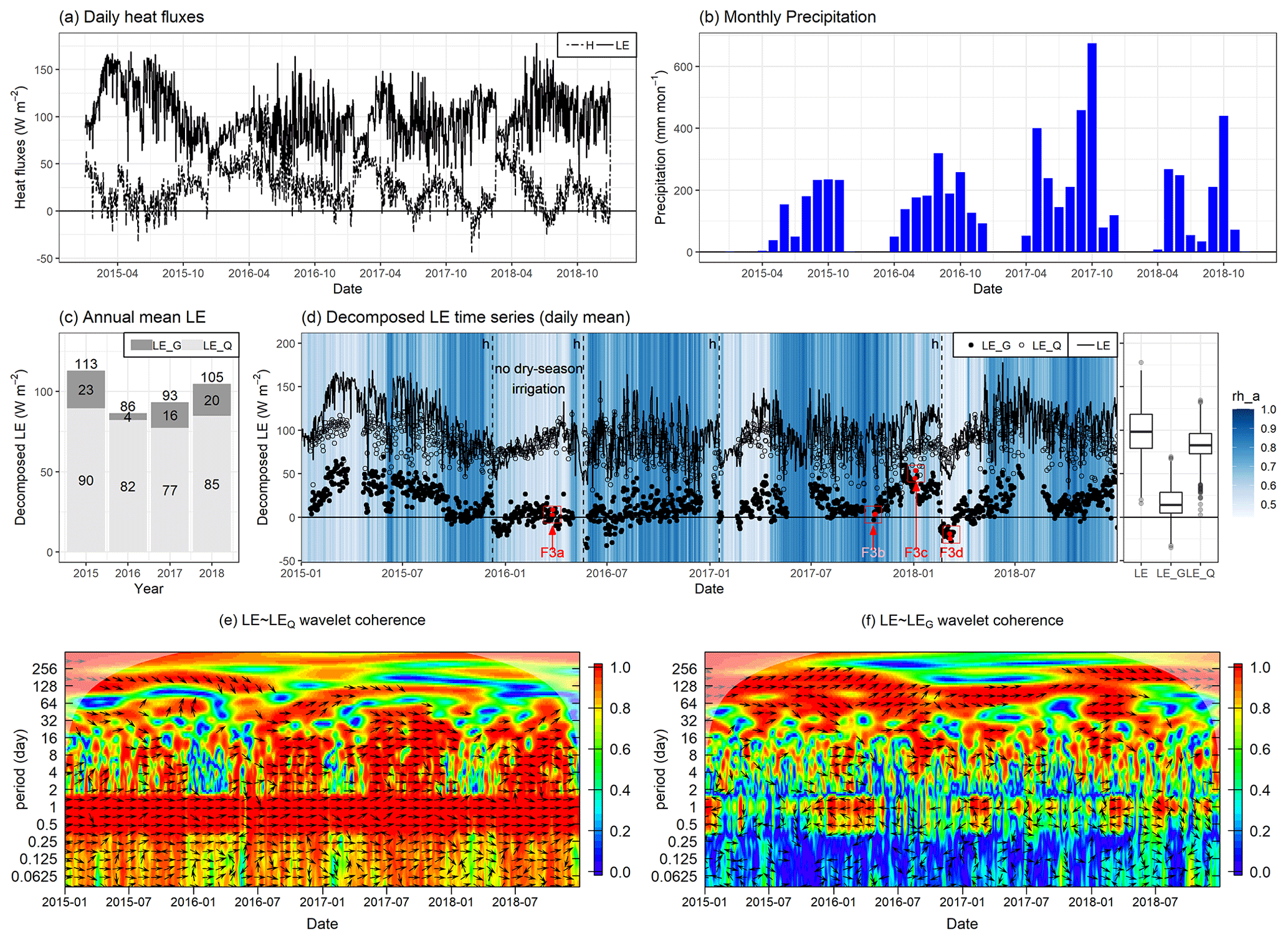
Figure 2Time series for the sugarcane EC tower site in Costa Rica. Panel (a) is daily heat fluxes and panel (b) is monthly precipitation. Panel (c) is mean annual LE and its two components, and (d) is time series of LE, LEQ, and LE with a background colour of RHa. Dashed lines with “h” in panel (d) indicate sugarcane harvest. Panels (e) and (f) are wavelet coherence of LE with LEQ and LE with LEG. Red and blue colours indicate high and low correlation, respectively. Arrows (pointing right: in-phase; left: antiphase) only appear when the coherence is significant (p < 0.01).
The measured LE and sensible heat flux (H) were quality controlled following Morillas et al. (2019) (details in the Supplement). For the study period, the surface energy balance closure (i.e., ) of 30 min data was 86 %, which is typical of high-quality eddy-covariance datasets (Wilson et al., 2002). When canopy height was less than 1 m, the surface energy balance was almost closed (97 %), whereas the closure was 83 % when canopy height was higher than 1 m. It is expected that unmeasured canopy and soil heat storages in this site are significant because the sugarcane canopy grew up to 3.6 m tall with a dense canopy. For instance, Meyers and Hollinger (2004) showed that storage term comprised 14 % of net radiation for a maize field with a 3 m canopy height and 8 % of net radiation for a soybean field with a 0.9 m canopy height, implying larger heat storage capacities for taller crop canopies. Also, since our study site is located within a homogenous landscape (Fig. S1 in the Supplement), horizontal and vertical advective flux divergence and the influence of secondary circulations on the energy balance closure may be marginal (Mauder et al., 2020; Leuning et al., 2012). Therefore, considering the homogenous landscape of the study site as well as a possible significant role of unmeasured canopy and soil heat storages, we did not force the energy closure. Consequently, we defined Q as the sum of LE and H instead of Rn−G. In doing so, we in effect attribute the cause of the surface energy imbalance to unmeasured heat storage terms following Moon et al. (2020).
In order to decompose LE into LEQ and LEG, we first estimated half-hourly aerodynamic resistance (ra) by considering aerodynamic resistance to momentum transfer and the additional boundary layer resistance for heat and mass transfer (or excess resistance) (Thom, 1972; Knauer et al., 2018a).
The first term on the right-hand side of Eq. (9) is the aerodynamic component, and the second term is the boundary layer component. Here, u∗ is friction velocity, k is the von Kármán constant (0.41), d is the zero-plane displacement height (d=0.7zh), z0 m is the roughness length for momentum (z0 m=0.1zh), and ψh is the integrated form of the stability correction function. zh is canopy height based on manual measurements taken during regular maintenance visits. ra was estimated using the bigleaf R package (Knauer et al., 2018a).
By rearranging Eq. (2), RHs can be calculated using
Negative H and inaccurate ra modelling sometimes yielded negative RHs or values greater than 1, especially at nighttime. In these cases, RHs was assigned the value of 1 following the approach described in the bigleaf R package (Knauer et al., 2018a). We then estimated LEQ and LEG from Eq. (4).
In order to explore the timescale of the covariances for LE ∼ LEQ and LE ∼ LEG in the frequency domain, we applied wavelet coherence analysis using the WaveletComp R package (Roesch and Schmidbauer, 2014). The package is designed to apply the continuous wavelet transform using the Morlet wavelet, which is a popular approach to analyze hydrological and micrometeorological datasets (Hatala et al., 2012; Johnson et al., 2013). A total time series of half-hourly decomposed LE for the 4-year measurement period was used to estimate localized coherence and phase angle. The wavelet coherence can be interpreted as the local correlation between two variables in the frequency–time domain (where red indicates high correlation). A 0∘ phase angle (arrow pointing right) indicates periods of positive correlation, while a 180∘ phase angle (arrow pointing left) indicates periods of negative correlation.
3.2 FLUXNET2015
The daily-scale FLUXNET2015 dataset, which includes 212 empirical eddy-covariance flux tower sites around the globe (Pastorello et al., 2020), was used in this study. The turbulent heat fluxes, net radiation, soil heat flux, air temperature, relative humidity, wind speed, friction velocity, and barometric pressure were obtained from the dataset. For this analysis, we only included daily data for periods for which the quality control flag indicated more than 80 % half-hourly data were present (i.e., measured data in general, or good-quality gap-filled data in cases of partially missing data).
In order to decompose daily LE into LEQ and LEG, we estimated daily aerodynamic resistance (ra) by Eq. (11) instead of Eq. (9) since canopy and measurement heights are unknown (Thom, 1972; Knauer et al., 2018a).
where u(zr) is reference height wind speed. ra was estimated using the bigleaf R package (Knauer et al., 2018a), and RHs was calculated from Eq. (8).
LEQ and LE were calculated using RHa and RHs following Eqs. (4) and (5), and then LEG and LE were calculated by subtracting LEQ and LE from LE. To calculate LEQ and LE, we define Q as LE + H, but it should be noted that this approach can include systematic uncertainty since the sum of LE and H measured by eddy covariance is typically lower than Rn−G (i.e., conditions referred to as the energy balance closure problem; Wilson et al., 2002). To investigate the effect of a lack of energy balance closure on resulting LE terms, we provide Fig. S2 that was generated by (1) defining Q as Rn−G and (2) correcting LE and H based on the assumption that the Bowen ratio () is correct (Pastorello et al., 2020).
3.3 FLUXCOM
The FLUXCOM dataset (Jung et al., 2019) is a global-scale machine learning ensemble product which upscales FLUXNET observations (Baldocchi et al., 2001) using Moderate Resolution Imaging Spectroradiometer (MODIS) satellite data and reanalysis meteorological data. In this study we used the monthly LE FLUXCOM dataset (0.5∘ resolution) modelled using MODIS and ECMWF ERA5 reanalysis data (Hersbach et al., 2020).
We obtained Q and LE from the FLUXCOM output, and air temperature and dew point temperature were retrieved from ERA5 monthly averaged data (2 m height). RH, S, and γ were calculated from ERA5 data, and then LE was calculated. LE was then estimated by subtracting LE from LE.
4.1 Decomposition analysis of in situ EC flux observation
Application results of the PMRH model to the observed LE at an irrigated sugarcane farm in Costa Rica are depicted in Fig. 2. The decomposition analysis of observed LE shows that while LEQ is the major component of LE, LEG variability plays a non-negligible role in seasonal and interannual behaviour of LE. In terms of absolute magnitude, the LEQ term can closely approximate LE, and LEG only represents 15 % of total evaporation (Fig. 2c). Also, positive coherence between LE and LEQ was strong over the entire period of observation, particularly at diurnal to multiday timescales (0.5–32 d), implying variability of LE is largely determined by LEQ variability (i.e., red coloured regions in Fig. 2e).
Although absolute magnitude of LEG was much smaller than that of LEQ, the interannual variability of LEG was larger than the interannual variability of LEQ (Fig. 2c). Furthermore, LE and LEG also had a strong positive correlation on longer timescales (32–365 d) (i.e., red coloured regions in Fig. 2f). Unexpectedly, a negative correlation between LE and LEG at the diurnal timescale was observed in the wavelet analysis only when the land surface was dry and there was little vegetation (i.e., after harvest) or during a year in which there was no dry season irrigation applied. Also, we found that EF variability is mostly determined by LEG variability since the diurnal and seasonal signals of Q are removed from LE in EF. Interestingly, the annual mean LEG was the highest in 2015, a drought year in which RHa and precipitation were generally lower than for the other years, while the annual mean LEG was close to zero in 2016 when there was no application of dry season irrigation due to crop replanting.
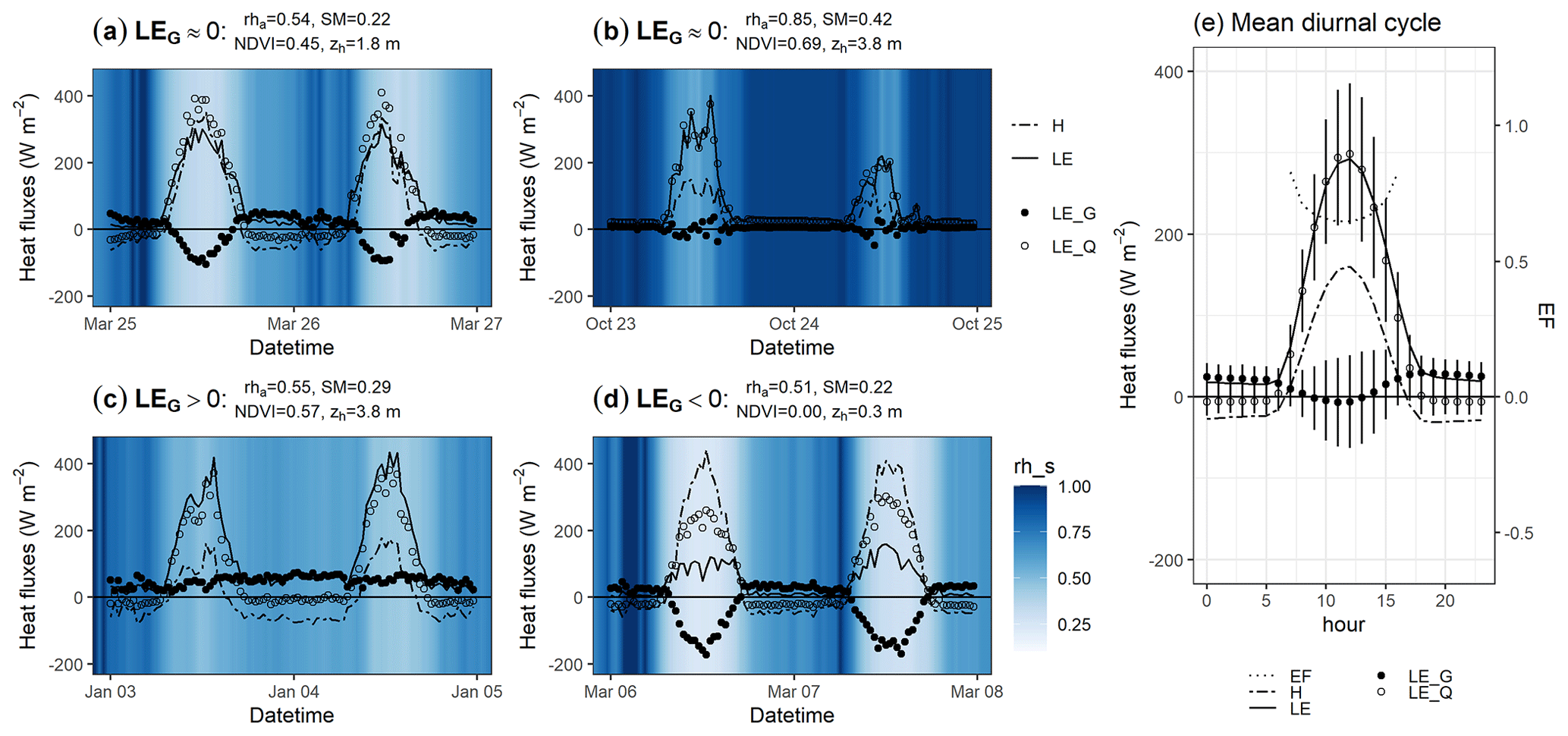
Figure 3Half-hourly time series of heat fluxes and the two components indicated in Fig. 2d. The background colour represents RHs. Here, RHa is mean atmospheric relative humidity, SM is volumetric soil water content, normalized difference vegetation index (NDVI) represents vegetation status, and zh is canopy height. Panel (e) presents the long-term mean diurnal cycle of decomposed LE (dots) and EF (dashed line).
To explore the diurnal behaviour of decomposed LE, we selected different surficial and atmospheric conditions when LEG was zero, positive, or negative in Fig. 3. In the 2016 dry season, LEG was close to zero as a daily average value, as a result of negative daytime and positive nighttime LEG values due to dry air and dry soil conditions (no irrigation) and an undeveloped vegetation canopy (Fig. 3a). Daily LEG was also close to zero during wet season conditions (e.g., Fig. 3b). In this case, LEG was near zero during both daytime and nighttime periods due to near-saturated atmospheric and land surface conditions. These two cases show that “dry land–dry air” or “wet land–wet air” conditions can each lead to daily scale land–atmosphere equilibrium, although the diurnal pattern of LEG is starkly different for dry land–dry air vs. wet land–wet air conditions.
Meanwhile, when RHa was low and the canopy was well-developed, LEG was found to be positive during both daytime and nighttime periods (Fig. 3c). On the other hand, during post-harvest conditions when vegetative canopy cover was minimal and air and soil moisture levels were low, daily LEG was found to be negative as a result of negative daytime and positive nighttime LEG (Fig. 3d). Diurnal variation in RHs was maximized when daily LEG was negative, implying a large diurnal fluctuation in surface temperature under the drier land surface conditions. Regarding the overall diurnal pattern, LEG generally declined during the morning and increased in the afternoon, which is consistent with the well-known diurnal pattern of EF (Gentine et al., 2011, 2007) (Fig. 3e).
4.2 Decomposition analysis of the FLUXNET2015 dataset
Decomposition analysis of the daily FLUXNET2015 dataset is illustrated in Fig. 4. In terms of absolute magnitude of each term, the majority of LEG (and LE) values ranged from −50 to 50 W m−2, with some exceptional values approaching ±100 W m−2. On the other hand, LEQ (and LE) values ranged from 0 to 150 W m−2.
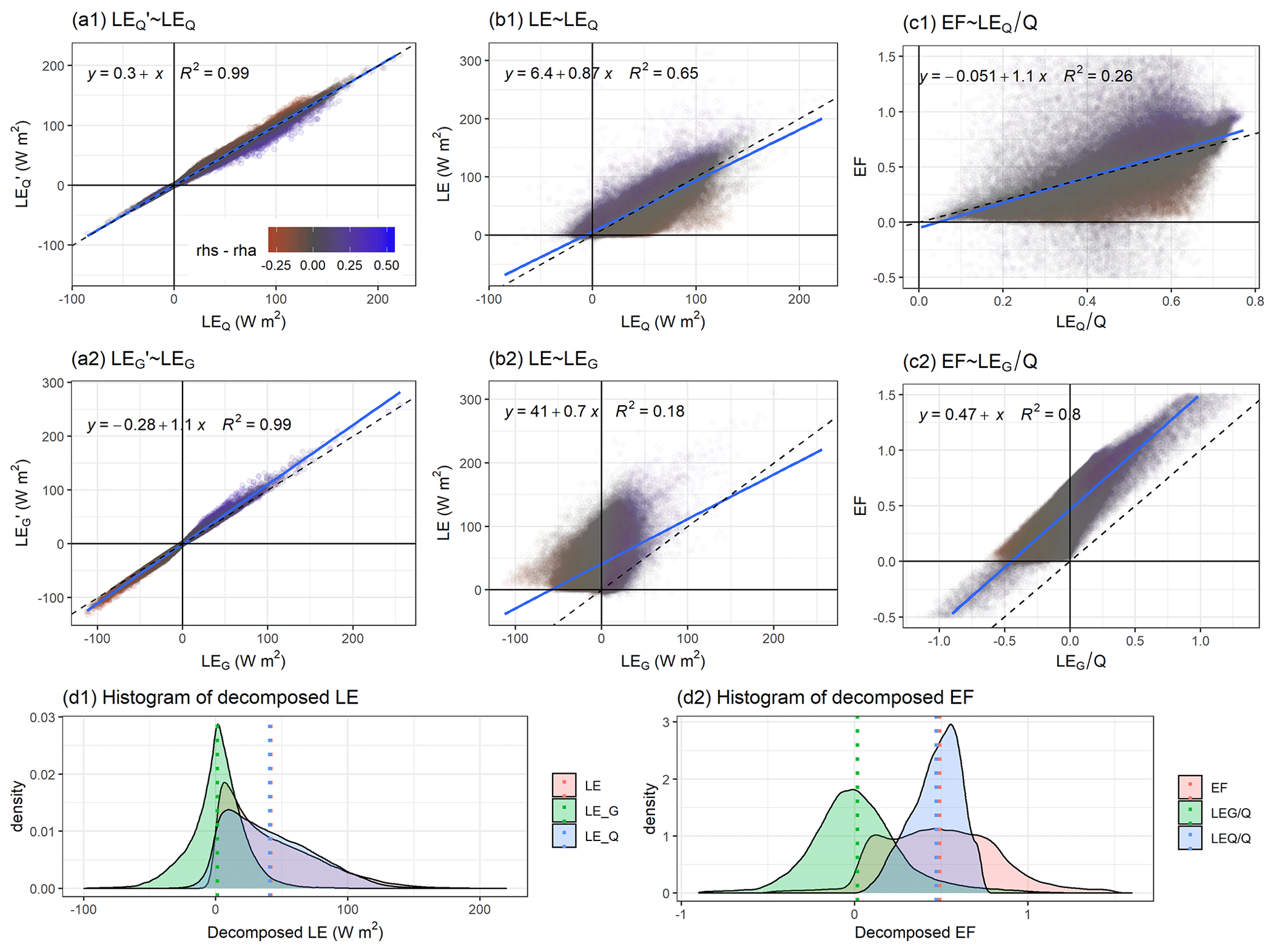
Figure 4FLUXNET2015 daily-scale decomposed LE for 212 sites and 1532 site years. Panels (a1) and (a2) are linear regressions of LE on LEQ and LE on LEG. Panels (b1) and (b2) are linear regressions of LE on LEQ and LE on LEG. Panels (c1) and (c2) are linear regressions of EF on LE and EF on LE. In these panels, daily EF data within a range from −1 to 1.5 are only shown. Here, dashed lines are one-to-one lines, blue lines are regression lines, and colour represents RHs − RHa. Panels (d1) and (d2) are histograms of decomposed LE and EF with mean values (dotted lines). To correct for lack of energy balance closure, Q was set equal to LE + H in all calculations.
One of the interesting findings from the decomposition analysis of the FLUXNET2015 dataset was that differences between LEQ and LE are marginal at a daily timescale (the slope is close to 1 in Fig. 4a1). This result implies that although the diabatic processes expressed by Eqs. (4) and (5) are different in magnitude due to the difference between RHs and RHa (see Sect. 2.3), these differences are practically negligible. This is an important point since LE can be determined simply and directly using reference height meteorological measurements, while LEQ is required to know RHs.
As for the adiabatic terms, LE is roughly 1.1 times LEG at a daily timescale (Fig. 4a2), which is consistent with the theory regarding their respective thermodynamic paths. As we discussed in Sect. 2.3, the absolute magnitude of LE must be bigger than that of LEG when available energy is positive. Therefore, the empirical relationship between LEG and LE in Fig. 4a2 is a consequence of a physical principle, and this result may provide the following empirical relationship.
Equation (12) reveals an emergent daily timescale relationship between temperature and relative humidity which has the potential to be used as a supplementary equation in future research.
Another important finding of the decomposition analysis is the global-scale land–atmosphere equilibrium. Our analysis in Fig. 4d1 indicates that the mean value of daily LEG of all FLUXNET2015 sites is close to zero, implying the global mean RH gradient is near zero at a daily timescale. Importantly, LE is primarily determined by LEQ (R2=0.65) instead of LEG (R2=0.18) as depicted in Fig. 4b1 and b2. Nevertheless, FLUXNET2015 data also suggest that LEG is the main driver of local-scale variability of EF at the daily timescale (Fig. 4c1 and c2). Although the mean value of daily EF is close to the mean value of , the variation in daily EF depends more on the variation in (Fig. 4d2). It should be noted that Figs. 4 and S2 are almost identical (Fig. S2 repeats the presentation shown in Fig. 4 using the value computed when forcing energy balance closure), implying that the lack of surface energy balance closure for EC observations does not significantly impact our analyses and interpretations.
4.3 Decomposition analysis of FLUXCOM dataset
We then applied the PMRH model to the FLUXCOM dataset, a benchmark global LE data product (Jung et al., 2019). As shown in Fig. 5a and c, the spatial patterns of the annual mean LE and LE were similar. For instance, both LE and LE show the highest values around the Equator at an annual timescale, which is mainly due to the energy available in this region. Also, spatial variability of LE is mostly determined by LE (R2=0.85 and slope = 1) rather than by LE (R2=0.18) (Fig. 5f1 and f2). This result is consistent with Eq. (8) and the SFE theory. In other words, the land surface is generally under thermodynamic equilibrium with the atmosphere at the global–annual scale (i.e., RHs≈RHa). Furthermore, the monthly time series of global LE and its two components in Fig. 5e1 show that (i) LE is consistently close to zero at the global scale and (ii) the seasonal variability of global LE is primarily determined by LE.
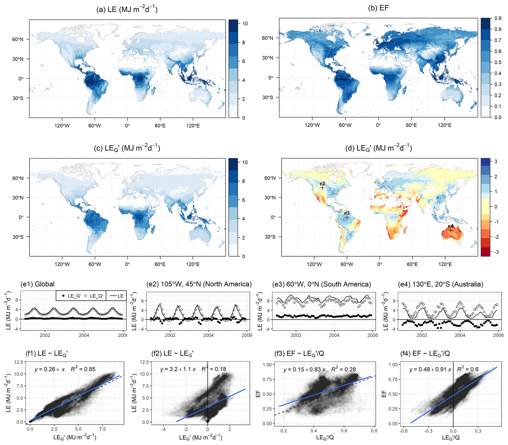
Figure 5Mean annual LE, EF, LE, and LE from 2001 to 2005 (panels a, b, c, and d, respectively). Panel (e1) is a time series of monthly global average LE and the two components LE and LE. Panels (e2), (e3), and (e4) are time series at specific locations highlighted in panel (d). Panels (f1), (f2), (f3), and (f4) are spatial linear regressions of LE on LE, LE on LE, EF on LE, and EF on LE, respectively.
However, while mean annual LE was close to zero in broad areas (particularly in high-latitude regions) as exemplified in Fig. 5e2, it was distinctly positive or negative at the annual scale for many regions (Fig. 5d). In humid tropical regions like the Amazon basin where moisture convergence is large, LE was generally positive, whereas arid regions such as Australia were characterized by negative LE (Fig. 5e3 and e4). Here, positive LE (i.e., RHs > RHa) indicates the land surface is wetter than the near-surface atmosphere while negative LE (i.e., RHs < RHa) implies a drier land surface than the atmosphere. Therefore, the sign of LE in Fig. 5d can be interpreted as representing land surface dryness relative to the atmosphere at an annual timescale.
The spatial pattern of LE is similar to the spatial pattern of EF, but differs from the spatial pattern of LE (Fig. 5b). For example, EF was high in not only tropical regions but also temperate climates such as Mediterranean regions, and this spatial pattern is well matched with the spatial pattern of LE but not LE. The finding that the spatial variation in EF is primarily controlled by LE instead of LE was supported by correlation analyses in Fig. 5f3 and f4 (R2=0.60 for EF ∼ and R2 = 0.28 for EF ∼ ). This is understandable in that EF is a reflection of the land surface dryness (Gentine et al., 2011), and LE reveals the land surface dryness relative to the atmosphere.
5.1 LEG at sub-daily scale
Salvucci and Gentine (2013) found that the variance of the RH gradient tends to be minimized over the course of the day. Based on this empirical finding, they developed an approach to predict LE only using standard meteorological measurements, and this approach accurately predicted actual LE (Rigden and Salvucci, 2015, 2017). Our PMRH model provides theoretical support for their approach in that LEG acts to reduce the RH gradient. Indeed, the U-shape diurnal cycles of LEG in Fig. 3 (positive nighttime and negative daytime) show the direction and the magnitude of the equilibration process of RH gradient at a sub-daily scale resulting in a small gradient of RH on daily average.
We found positive nighttime LEG values regardless of wet or dry conditions, except when the atmosphere was fully saturated (Fig. 3). This result is a natural consequence since the land surface is close to saturation at night. This finding suggests that LEG is a dominant contributor to nighttime evaporation since available energy is close to zero at night. It is important since nighttime evaporation is a non-negligible component of total ET (Padrón et al., 2020).
Unlike nighttime LEG values, the direction and the magnitude of the daytime LEG are highly dependent on the land surface dryness. For example, the U-shape diurnal cycles of LEG are apparent only when the land surface is dry, which is confirmed by the negative wavelet coherence between LE and LEG at the diurnal timescale in Fig. 2f. When the land surface is wetter than the atmosphere, LEG values were positive even in the daytime, and thus the U-shape diurnal cycles of LEG did not appear (Fig. 3c). The positive LEG during daytime periods may be explained as a consequence of warm and dry air entrainment at the top of the atmospheric boundary layer and/or horizontal advection of sensible heat which may reduce atmospheric relative humidity (Baldocchi et al., 2016; de Bruin et al., 2016). Indeed, a strong entrainment effect and/or local advection of sensible heat are common phenomena for irrigated agriculture (Baldocchi et al., 2016; de Bruin and Trigo, 2019), and the irrigated sugarcane site shows that the annual mean LEG was always positive except for in 2016 when there was no application of dry season irrigation.
5.2 LEG at daily to annual timescales
As described in the theory section, land–atmosphere equilibrium is achieved when LEG approaches zero and thus LE reduces to Eq. (8) at a timescale longer than sub-daily. The decomposed terms derived from both the empirical FLUXNET2015 and model-based FLUXCOM datasets show that the global mean for LEG is near zero, implying global-scale land–atmosphere equilibrium (Figs. 4 and 5). This result extends the SFE theory of McColl et al. (2019). Although LEG is not always near zero for timescales longer than sub-daily, moisture convergence and divergence at the global scale tend to balance each other out, resulting in global-scale land–atmosphere equilibrium on longer timescales (Fig. 5e1).
From a different perspective, non-zero LEG value and its sign (+ vs. −) at the local scale can be understood as an indicator reflecting land surface dryness relative to the atmosphere. We found that LEG clearly distinguishes spatially wet and dry regions around the world (Fig. 5 d). We also found that the spatiotemporal variability of EF was largely explained by LEG instead of LEQ (Figs. 4c2 and 5f4). These results demonstrate the usefulness of LEG to quantify land surface dryness. Some previous studies introduced evaporative stress index or evaporation deficit index based on the ratio (or difference) between potential evaporation and actual evaporation (Anderson et al., 2015; Kim and Rhee, 2016; Fisher et al., 2020; Baldocchi et al., 2021), but these methods are highly dependent on the way one calculates potential evaporation. Unlike potential evaporation (which is a theoretical value), LEG is a true physical quantity, and negative LEG values directly reflect water-limited land surface conditions. Therefore, we suggest applying our decomposition method to better quantify evaporative stress.
5.3 Future applications
In this study, we present the PMRH model and demonstrate its utility for exploratory and diagnostic purposes. However, the model has potential applications for other purposes. One possible application is to use PMRH to predict actual ET. Although the original PM equation is widely used to predict evapotranspiration (e.g., Leuning et al., 2008; Mu et al., 2011; Mallick et al., 2014), its accuracy often relies on parameterized surface resistance models (Polhamus et al., 2013). Since our PMRH formulation does not include surface resistance, it could represent a good alternative. As shown in the results section, LE can be calculated using typical meteorological data without additional surface parameters. Also, we found that LE alone can be used effectively to approximate LE. If the remotely sensed land surface conditions are known (e.g., soil moisture and/or land surface temperature), actual LE may be more accurately predicted by incorporating the LEG term. To estimate the LEG term, RHs may be estimated based on soil moisture and/or land surface temperature data. For example, Eq. (12), which is well supported by observations (Fig. 4a2) and on a physical basis, may be used to calculate RHs.
Another possible application is to study impacts of climate change and land use and land cover change on surface energy partitioning and evaporation. Changes in the atmospheric state such as temperature and relative humidity, as well as changes in the land surface characteristics such as albedo and aerodynamic roughness, can alter evaporation (Lee et al., 2011; Wang et al., 2018). However, how these changes affect terrestrial energy partitioning and ET is still unclear. Indeed, there is a large discrepancy in long-term LE trends among current land surface models (Pan et al., 2020). Since PMRH makes it possible to physically decompose LE into adiabatic and diabatic thermodynamic components, the PMRH approach can be useful to understand how environmental changes affect surface energy partitioning. For instance, trend analysis for the decomposed LE using PMRH could contribute to improve our understanding of earth's climate system and water cycle.
5.4 Potential caveats
Despite the insights it can offer, the PMRH model shares several limitations with the traditional PM model. First, PM-style equations linearize the exponential relationship between saturation vapour pressure and temperature (Clausius–Clapeyron relation), but the linearization can cause bias when the temperature difference between surface and atmosphere is substantial (Paw U and Gao, 1988; McColl, 2020). Second, the PMRH model assumes that aerodynamic resistance for heat and water vapour is identical, which implicitly relies on the assumption that the ratio of the turbulent Schmidt to Prandtl numbers is unity (Knauer et al., 2018a). This similarity assumption cannot be held in some cases, especially when advective flux divergence is significant (Lee et al., 2004). The third potential caveat is that we define the land surface as an idealized single plane that is equivalent to the “bigleaf” representation of the traditional PM equation, but this approach ignores profiles of temperature and humidity inside the canopy (Bonan et al., 2021).
Another potential caveat concerns the surface energy balance. The surface energy balance is a governing equation of the PM-style models, but it is not satisfied in typical EC observations, which is referred to as the “surface energy balance closure problem” (Wilson et al., 2002). This closure problem could cause a systematic uncertainty in estimating rs when using the PM equation (Knauer et al., 2018b; Wohlfahrt et al., 2009), and this issue may affect the diagnostic analyses using the PMRH. In this study, we did not force the energy balance closure and attributed the cause of observed surface energy imbalances to unmeasured heat storage terms for the Costa Rica EC site due to the possibly significant role of the heat storage term (details in the Sect. 3.1). Wehr and Saleska (2021) recently demonstrated that regardless of whether the lack of energy balance closure of EC observations is due to LE+H or is due to Rn−G, applying the flux gradient equation to observed LE and H without energy balance correction is the best way to determine rs. This is because applying the flux gradient equation to observed LE and H can dispense with the unnecessary assumption of energy balance closure. They showed that bias introduced by underestimated LE and H is smaller than the bias introduced by the energy balance closure assumption. This finding may be applied to our analysis in calculating RHs instead of rs.
As for the FLUXNET2015 dataset, we provide an alternate analysis using energy-balance-corrected LE and H (Bowen ratio preserving method in Pastorello et al., 2020) in the Supplement. We found that the results for corrected and uncorrected versions were almost identical, which can be viewed as a natural consequence since in Eq. (10) LE and H are included in the numerator and denominator respectively. Multiplying the same ratio to LE and H in Eq. (10) to correct LE and H based on the Bowen ratio method does not significantly change the resulting RHs. Therefore, the lack of surface energy balance closure does not significantly impact our analyses and interpretations unless the lack of energy balance is dominated by LE only or H only. If the lack of energy balance is dominated by LE only or H only, our results and interpretation may include systematic bias.
Finally, there are several ways to calculate aerodynamic resistance, and the chosen form for ra may affect the results. However, the influence of this choice is expected to be marginal compared to the energy balance problem. Knauer et al. (2018b) showed that uncertainty caused by different ra values on surface conductance is low compared to the energy balance closure problem. This finding can be applied to our analysis. Specifically, in Eq. (10), ra is multiplied by both denominator and numerator, and thus a small difference in ra should not significantly affect the resulting RHs.
We have shown that our novel PMRH model provides a new opportunity to understand the governing physics of the terrestrial energy budget. Specifically, the PMRH model helps to illustrate how the land surface conditions become encoded to the atmospheric state by partitioning LE into two thermodynamic processes. “Dry land–dry air” or “wet land–wet air” conditions can each lead to daily scale land–atmosphere equilibrium, although the diurnal pattern of the equilibration process (i.e., LEG) is starkly different. Our findings suggest that while LEG is a primary component determining EF, spatiotemporal variability of LEQ alone can adequately represent the variability of LE. We found global-scale land–atmosphere equilibrium at daily to annual scales, which implies that global LE can be simply determined by the atmospheric state and radiative energy without any surface constraint required to represent spatial heterogeneity and physiological influences. From a different perspective, the non-zero LEG value at a local scale can be understood as an indicator revealing land surface dryness. Questions remain regarding how LEQ and LEG will be influenced in relation to changing climatic and land surface conditions and how these changes might affect the climate system at differing spatial and temporal scales through positive or negative feedbacks.
The FLUXNET2015 dataset is available in https://fluxnet.org/data/download-data/ (FLUXET community, 2019). The highlighted sugarcane eddy covariance site dataset will be available in AmeriFlux (by December 2021, https://ameriflux.lbl.gov/, AmeriFlux, 2021). The FLUXCOM dataset is available in http://www.fluxcom.org/EF-Download/ (FLUXCOM, 2021).
The supplement related to this article is available online at: https://doi.org/10.5194/hess-25-5175-2021-supplement.
YK and MSJ designed research; UW provided FLUXCOM data; YK, LM, and MSJ performed research; YK analyzed data; YK, MG, TAB, LM, and MSJ wrote the paper.
The authors declare that they have no conflict of interest.
Publisher's note: Copernicus Publications remains neutral with regard to jurisdictional claims in published maps and institutional affiliations.
We want to thank Iain Hawthorne, Pável Bautista, Silja Hund, Cameron Webster, Gretel Rojas Hernandez, Guillermo Duran Sanabria, Andrea Suarez Serrano, Ana Maria Duran, Martin Martinez, and Fermín Subirós Ruiz for field and logistical support. We also thank Martin Jung, the principal investigator of the FLUXCOM dataset. The authors would like to thank the EU and NSERC for funding, in the frame of the collaborative international Consortium AgWIT financed under the ERA-NET WaterWorks2015 Cofunded Call. This ERA-NET is an integral part of the 2016 Joint Activities developed by the Water Challenges for a Changing World Joint Programme Initiative (Water JPI).
This research has been supported by the Joint Programming Initiative Water challenges for a changing world (Agricultural Water Innovations in the Tropics).
This paper was edited by Anke Hildebrandt and reviewed by two anonymous referees.
Ameriflux: CR-Fsc site (Filadelfia sugar cane cropland), available at: https://ameriflux.lbl.gov/, last access: 22 September 2021.
Anderson, M. C., Zolin, C. A., Hain, C. R., Semmens, K., Tugrul Yilmaz, M., and Gao, F.: Comparison of satellite-derived LAI and precipitation anomalies over Brazil with a thermal infrared-based Evaporative Stress Index for 2003–2013, J. Hydrol., 526, 287–302, https://doi.org/10.1016/j.jhydrol.2015.01.005, 2015.
Baldocchi, D., Falge, E., Gu, L., Olson, R., Hollinger, D., Running, S., Anthoni, P., Bernhofer, C., Davis, K., and Evans, R.: FLUXNET: A new tool to study the temporal and spatial variability of ecosystem-scale carbon dioxide, water vapor, and energy flux densities, B. Am. Meteorol. Soc., 82, 2415–2434, https://doi.org/10.1175/1520-0477(2001)082<2415:FANTTS>2.3.CO;2, 2001.
Baldocchi, D., Knox, S., Dronova, I., Verfaillie, J., Oikawa, P., Sturtevant, C., Matthes, J. H., and Detto, M.: The impact of expanding flooded land area on the annual evaporation of rice, Agr. Forest Meteorol., 223, 181–193, https://doi.org/10.1016/j.agrformet.2016.04.001, 2016.
Baldocchi, D., Ma, S., and Verfaillie, J.: On the inter- and intra-annual variability of ecosystem evapotranspiration and water use efficiency of an oak savanna and annual grassland subjected to booms and busts in rainfall, Glob. Change Biol., 27, 359–375, https://doi.org/10.1111/gcb.15414, 2021.
Bonan, G. B., Patton, E. G., Finnigan, J. J., Baldocchi, D. D., and Harman, I. N.: Moving beyond the incorrect but useful paradigm: reevaluating big-leaf and multilayer plant canopies to model biosphere-atmosphere fluxes – a review, Agr. Forest Meteorol., 306, 108435, https://doi.org/10.1016/j.agrformet.2021.108435, 2021.
Bouchet, R. J.: Evapotranspiration réelle et potentielle, signification climatique, IAHS Publ, 62, 134–142, 1963.
Byrne, M. P. and O'Gorman, P. A.: Understanding Decreases in Land Relative Humidity with Global Warming: Conceptual Model and GCM Simulations, J. Climate, 29, 9045–9061, https://doi.org/10.1175/jcli-d-16-0351.1, 2016.
Byrne, M. P. and O'Gorman, P. A.: Trends in continental temperature and humidity directly linked to ocean warming, P. Natl. Acad. Sci. USA, 115, 4863–4868, https://doi.org/10.1073/pnas.1722312115, 2018.
Chen, S., McColl, K. A., Berg, A., and Huang, Y.: Surface flux equilibrium estimates of evapotranspiration at large spatial scales, J. Hydrometeorol., 22, 765–779, https://doi.org/10.1175/jhm-d-20-0204.1, 2021.
Cuxart, J. and Boone, A. A.: Evapotranspiration over Land from a Bound.-Lay. Meteorol. Perspective, Bound.-Lay. Meteorol., 177, 427–459, https://doi.org/10.1007/s10546-020-00550-9, 2020.
de Bruin, H. and Trigo, I.: A new method to estimate reference crop evapotranspiration from geostationary satellite imagery: Practical considerations, Water, 11, 382, https://doi.org/10.3390/w11020382, 2019.
de Bruin, H. A. R., Trigo, I. F., Bosveld, F. C., and Meirink, J. F.: A Thermodynamically Based Model for Actual Evapotranspiration of an Extensive Grass Field Close to FAO Reference, Suitable for Remote Sensing Application, J. Hydrometeorol., 17, 1373–1382, https://doi.org/10.1175/jhm-d-15-0006.1, 2016.
Eichinger, W. E., Parlange, M. B., and Stricker, H.: On the concept of equilibrium evaporation and the value of the Priestley-Taylor coefficient, Water Resour. Res., 32, 161–164, https://doi.org/10.1029/95wr02920, 1996.
Emanuel, K.: The Relevance of Theory for Contemporary Research in Atmospheres, Oceans, and Climate, AGU Advances, 1, e2019AV000129, https://doi.org/10.1029/2019AV000129, 2020.
Fisher, J. B., Tu, K. P., and Baldocchi, D. D.: Global estimates of the land–atmosphere water flux based on monthly AVHRR and ISLSCP-II data, validated at 16 FLUXNET sites, Remote Sens. Environ., 112, 901–919, https://doi.org/10.1016/j.rse.2007.06.025, 2008.
Fisher, J. B., Lee, B., Purdy, A. J., Halverson, G. H., Dohlen, M. B., Cawse-Nicholson, K., Wang, A., Anderson, R. G., Aragon, B., Arain, M. A., Baldocchi, D. D., Baker, J. M., Barral, H., Bernacchi, C. J., Bernhofer, C., Biraud, S. C., Bohrer, G., Brunsell, N., Cappelaere, B., Castro-Contreras, S., Chun, J., Conrad, B. J., Cremonese, E., Demarty, J., Desai, A. R., De Ligne, A., Foltýnová, L., Goulden, M. L., Griffis, T. J., Grünwald, T., Johnson, M. S., Kang, M., Kelbe, D., Kowalska, N., Lim, J.-H., Maïnassara, I., McCabe, M. F., Missik, J. E. C., Mohanty, B. P., Moore, C. E., Morillas, L., Morrison, R., Munger, J. W., Posse, G., Richardson, A. D., Russell, E. S., Ryu, Y., Sanchez-Azofeifa, A., Schmidt, M., Schwartz, E., Sharp, I., Šigut, L., Tang, Y., Hulley, G., Anderson, M., Hain, C., French, A., Wood, E., and Hook, S.: ECOSTRESS: NASA's Next Generation Mission to Measure Evapotranspiration From the International Space Station, Water Resour. Res., 56, e2019WR026058, https://doi.org/10.1029/2019wr026058, 2020.
FLUXCOM: FLUXCOM energy flux data, available at: http://www.fluxcom.org/EF-Download/, last access: 16 April 2020.
FLUXET community: FLUXNET2015 SUBSET data, available at: https://fluxnet.org/data/download-data/, last access: 19 November 2019.
García, M., Sandholt, I., Ceccato, P., Ridler, M., Mougin, E., Kergoat, L., Morillas, L., Timouk, F., Fensholt, R., and Domingo, F.: Actual evapotranspiration in drylands derived from in situ and satellite data: Assessing biophysical constraints, Remote Sens. Environ., 131, 103–118, https://doi.org/10.1016/j.rse.2012.12.016, 2013.
Gentine, P., Entekhabi, D., Chehbouni, A., Boulet, G., and Duchemin, B.: Analysis of evaporative fraction diurnal behaviour, Agr. Forest Meteorol., 143, 13–29, https://doi.org/10.1016/j.agrformet.2006.11.002, 2007.
Gentine, P., Entekhabi, D., and Polcher, J.: The Diurnal Behavior of Evaporative Fraction in the Soil–Vegetation–Atmospheric Boundary Layer Continuum, J. Hydrometeorol., 12, 1530–1546, https://doi.org/10.1175/2011jhm1261.1, 2011.
Hatala, J. A., Detto, M., and Baldocchi, D. D.: Gross ecosystem photosynthesis causes a diurnal pattern in methane emission from rice, Geophys. Res. Lett., 39, 1–5, https://doi.org/10.1029/2012GL051303, 2012.
Hersbach, H., Bell, B., Berrisford, P., Hirahara, S., Horányi, A., Muñoz-Sabater, J., Nicolas, J., Peubey, C., Radu, R., and Schepers, D.: The ERA5 global reanalysis, Q. J. Roy. Meteor. Soc., 146, 1999–2049, 2020.
Hund, S. V., Allen, D. M., Morillas, L., and Johnson, M. S.: Groundwater recharge indicator as tool for decision makers to increase socio-hydrological resilience to seasonal drought, J. Hydrol., 563, 1119–1134, https://doi.org/10.1016/j.jhydrol.2018.05.069, 2018.
Iribarne, J. V. and Godson, W. L.: Atmospheric Thermodynamics, in: Geophysics and Astrophysics Monographs, 2nd Edn., edited by: McCormac, B. M., Kluwer Academic Publishers, Boston, 1981.
Jarvis, P. G. and McNaughton, K. G.: Stomatal control of transpiration: Scaling up from leaf to region, in: Advances in Ecological Research, edited by: MacFadyen, A. and Ford, E. D., Academic Press, Cambridge, USA, 1–49, 1986.
Johnson, M. S., Couto, E. G., Pinto Jr., O. B., Milesi, J., Santos Amorim, R. S., Messias, I. A. M., and Biudes, M. S.: Soil CO2 Dynamics in a Tree Island Soil of the Pantanal: The Role of Soil Water Potential, PLOS ONE, 8, e64874, https://doi.org/10.1371/journal.pone.0064874, 2013.
Jung, M., Koirala, S., Weber, U., Ichii, K., Gans, F., Camps-Valls, G., Papale, D., Schwalm, C., Tramontana, G., and Reichstein, M.: The FLUXCOM ensemble of global land-atmosphere energy fluxes, Scientific Data, 6, 74, https://doi.org/10.1038/s41597-019-0076-8, 2019.
Kim, D. and Rhee, J.: A drought index based on actual evapotranspiration from the Bouchet hypothesis, Geophys. Res. Lett., 43, 10277–10285, https://doi.org/10.1002/2016GL070302, 2016.
Kleidon, A. and Schymanski, S.: Thermodynamics and optimality of the water budget on land: A review, Geophys. Res. Lett., 35, L20404, https://doi.org/10.1029/2008gl035393, 2008.
Kleidon, A., Schymanski, S., and Stieglitz, M.: Thermodynamics, Irreversibility, and Optimality in Land Surface Hydrology, in: Bioclimatology and Natural Hazards, edited by: Střelcová, K., Mátyás, C., Kleidon, A., Lapin, M., Matejka, F., Blaženec, M., Škvarenina, J., and Holécy, J., Springer Netherlands, Dordrecht, the Netherlands, 107–118, 2009.
Knauer, J., El-Madany, T. S., Zaehle, S., and Migliavacca, M.: Bigleaf – An R package for the calculation of physical and physiological ecosystem properties from eddy covariance data, PLOS ONE, 13, e0201114, https://doi.org/10.1371/journal.pone.0201114, 2018a.
Knauer, J., Zaehle, S., Medlyn, B. E., Reichstein, M., Williams, C. A., Migliavacca, M., Kauwe, M. G. D., Werner, C., Keitel, C., Kolari, P., Limousin, J. M., and Linderson, M. L.: Towards physiologically meaningful water-use efficiency estimates from eddy covariance data, Glob. Change Biol., 24, 694–710, https://doi.org/10.1111/gcb.13893, 2018b.
Lee, T. J. and Pielke, R. A.: Estimating the soil surface specific humidity, J. Appl. Meteorol. Clim., 31, 480–484, 1992.
Lee, X., Yu, Q., Sun, X., Liu, J., Min, Q., Liu, Y., and Zhang, X.: Micrometeorological fluxes under the influence of regional and local advection: a revisit, Agr. Forest Meteorol., 122, 111–124, https://doi.org/10.1016/j.agrformet.2003.02.001, 2004.
Lee, X., Goulden, M. L., Hollinger, D. Y., Barr, A., Black, T. A., Bohrer, G., Bracho, R., Drake, B., Goldstein, A., Gu, L., Katul, G., Kolb, T., Law, B. E., Margolis, H., Meyers, T., Monson, R., Munger, W., Oren, R., Paw U, K. T., Richardson, A. D., Schmid, H. P., Staebler, R., Wofsy, S., and Zhao, L.: Observed increase in local cooling effect of deforestation at higher latitudes, Nature, 479, 384–387, https://doi.org/10.1038/nature10588, 2011.
Leuning, R., Zhang, Y. Q., Rajaud, A., Cleugh, H., and Tu, K.: A simple surface conductance model to estimate regional evaporation using MODIS leaf area index and the Penman-Monteith equation, Water Resour. Res., 44, W10419, https://doi.org/10.1029/2007wr006562, 2008.
Leuning, R., van Gorsel, E., Massman, W. J., and Isaac, P. R.: Reflections on the surface energy imbalance problem, Agr. Forest Meteorol., 156, 65–74, https://doi.org/10.1016/j.agrformet.2011.12.002, 2012.
Li, D. and Wang, L.: Sensitivity of surface temperature to land use and land cover change-Induced biophysical changes: the scale Issue, Geophys. Res. Lett., 46, 9678–9689, https://doi.org/10.1029/2019gl084861, 2019.
Lovell-Smith, J. W., Feistel, R., Harvey, A. H., Hellmuth, O., Bell, S. A., Heinonen, M., and Cooper, J. R.: Metrological challenges for measurements of key climatological observables. Part 4: atmospheric relative humidity, Metrologia, 53, R40–R59, https://doi.org/10.1088/0026-1394/53/1/r40, 2015.
Ma, H.-Y., Klein, S. A., Xie, S., Zhang, C., Tang, S., Tang, Q., Morcrette, C. J., Van Weverberg, K., Petch, J., Ahlgrimm, M., Berg, L. K., Cheruy, F., Cole, J., Forbes, R., Gustafson Jr., W. I., Huang, M., Liu, Y., Merryfield, W., Qian, Y., Roehrig, R., and Wang, Y.-C.: CAUSES: On the Role of Surface Energy Budget Errors to the Warm Surface Air Temperature Error Over the Central United States, J. Geophys. Res.-Atmos., 123, 2888–2909, https://doi.org/10.1002/2017jd027194, 2018.
Mallick, K., Jarvis, A. J., Boegh, E., Fisher, J. B., Drewry, D. T., Tu, K. P., Hook, S. J., Hulley, G., Ardö, J., Beringer, J., Arain, A., and Niyogi, D.: A Surface Temperature Initiated Closure (STIC) for surface energy balance fluxes, Remote Sens. Environ., 141, 243–261, https://doi.org/10.1016/j.rse.2013.10.022, 2014.
Marsh, A.: Psychrometric Chart, available at: https://drajmarsh.bitbucket.io/psychro-chart2d.html (last access: 22 September 2020), 2018.
Martens, B., Miralles, D. G., Lievens, H., van der Schalie, R., de Jeu, R. A. M., Fernández-Prieto, D., Beck, H. E., Dorigo, W. A., and Verhoest, N. E. C.: GLEAM v3: satellite-based land evaporation and root-zone soil moisture, Geosci. Model Dev., 10, 1903–1925, https://doi.org/10.5194/gmd-10-1903-2017, 2017.
Massmann, A., Gentine, P., and Lin, C.: When Does Vapor Pressure Deficit Drive or Reduce Evapotranspiration?, J. Adv. Model. Earth Syst., 11, 3305–3320, https://doi.org/10.1029/2019ms001790, 2019.
Mauder, M., Foken, T., and Cuxart, J.: Surface-Energy-Balance Closure over Land: A Review, Bound.-Lay. Meteorol., 177, 395–426, https://doi.org/10.1007/s10546-020-00529-6, 2020.
McColl, K. A.: Practical and theoretical benefits of an alternative to the Penman-Monteith evapotranspiration equation, Water Resour. Res., 56, e2020WR027106, https://doi.org/10.1029/2020wr027106, 2020.
McColl, K. A. and Rigden, A. J.: Emergent Simplicity of Continental Evapotranspiration, Geophys. Res. Lett., 47, e2020GL087101, https://doi.org/10.1029/2020gl087101, 2020.
McColl, K. A., Salvucci, G. D., and Gentine, P.: Surface flux equilibrium theory explains an empirical estimate of water-limited daily evapotranspiration, J. Adv. Model. Earth Syst., 11, 2036–2049, https://doi.org/10.1029/2019ms001685, 2019.
McNaughton, K. and Spriggs, T.: An evaluation of the Priestley and Taylor equation and the complementary relationship using results from a mixed-layer model of the convective boundary layer, IAHS publication, 177, 89–104, 1989.
McNaughton, K. G. and Jarvis, P. G.: Predicting effects of vegetation changes on transpiration and evaporation, Water deficits and plant growth, 7, 1–47, 1983.
Meyers, T. P. and Hollinger, S. E.: An assessment of storage terms in the surface energy balance of maize and soybean, Agr. Forest Meteorol., 125, 105–115, https://doi.org/10.1016/j.agrformet.2004.03.001, 2004.
Monteith, J. L.: Evaporation and environment. The state and movement of water in living organisms, Symposium of the society of experimental biology, 19, 205–234, 1965.
Monteith, J. L.: Evaporation and surface temperature, Q. J. Roy. Meteor. Soc., 107, 1–27, https://doi.org/10.1002/qj.49710745102, 1981.
Monteith, J. L. and Unsworth, M.: Principles of environmental physics: plants, animals, and the atmosphere, Academic Press, Oxford, 2013.
Moon, M., Li, D., Liao, W., Rigden, A. J., and Friedl, M. A.: Modification of surface energy balance during springtime: The relative importance of biophysical and meteorological changes, Agr. Forest Meteorol., 284, 107905, https://doi.org/10.1016/j.agrformet.2020.107905, 2020.
Morillas, L., Hund, S. V., and Johnson, M. S.: Water Use Dynamics in Double Cropping of Rainfed Upland Rice and Irrigated Melons Produced Under Drought-Prone Tropical Conditions, Water Resour. Res., 55, 4110–4127, https://doi.org/10.1029/2018wr023757, 2019.
Mu, Q., Zhao, M., and Running, S. W.: Improvements to a MODIS global terrestrial evapotranspiration algorithm, Remote Sens. Environ., 115, 1781–1800, https://doi.org/10.1016/j.rse.2011.02.019, 2011.
Novick, K. A. and Katul, G. G.: The Duality of Reforestation Impacts on Surface and Air Temperature, J. Geophys. Res.-Biogeo., 125, e2019JG005543, https://doi.org/10.1029/2019jg005543, 2020.
Novick, K. A., Ficklin, D. L., Stoy, P. C., Williams, C. A., Bohrer, G., Oishi, A. C., Papuga, S. A., Blanken, P. D., Noormets, A., Sulman, B. N., Scott, R. L., Wang, L., and Phillips, R. P.: The increasing importance of atmospheric demand for ecosystem water and carbon fluxes, Nat. Clim. Change, 6, 1023, https://doi.org/10.1038/nclimate3114, 2016.
Oki, T. and Kanae, S.: Global hydrological cycles and world water resources, Science, 313, 1068–1072, 2006.
Padrón, R. S., Gudmundsson, L., Michel, D., and Seneviratne, S. I.: Terrestrial water loss at night: global relevance from observations and climate models, Hydrol. Earth Syst. Sci., 24, 793–807, https://doi.org/10.5194/hess-24-793-2020, 2020.
Pan, S., Pan, N., Tian, H., Friedlingstein, P., Sitch, S., Shi, H., Arora, V. K., Haverd, V., Jain, A. K., Kato, E., Lienert, S., Lombardozzi, D., Nabel, J. E. M. S., Ottlé, C., Poulter, B., Zaehle, S., and Running, S. W.: Evaluation of global terrestrial evapotranspiration using state-of-the-art approaches in remote sensing, machine learning and land surface modeling, Hydrol. Earth Syst. Sci., 24, 1485–1509, https://doi.org/10.5194/hess-24-1485-2020, 2020.
Pastorello, G., Trotta, C., Canfora, E., Chu, H., Christianson, D., Cheah, Y.-W., Poindexter, C., Chen, J., Elbashandy, A., Humphrey, M., Isaac, P., Polidori, D., Ribeca, A., van Ingen, C., Zhang, L., Amiro, B., Ammann, C., Arain, M. A., Ardö, J., Arkebauer, T., Arndt, S. K., Arriga, N., Aubinet, M., Aurela, M., Baldocchi, D., Barr, A., Beamesderfer, E., Marchesini, L. B., Bergeron, O., Beringer, J., Bernhofer, C., Berveiller, D., Billesbach, D., Black, T. A., Blanken, P. D., Bohrer, G., Boike, J., Bolstad, P. V., Bonal, D., Bonnefond, J.-M., Bowling, D. R., Bracho, R., Brodeur, J., Brümmer, C., Buchmann, N., Burban, B., Burns, S. P., Buysse, P., Cale, P., Cavagna, M., Cellier, P., Chen, S., Chini, I., Christensen, T. R., Cleverly, J., Collalti, A., Consalvo, C., Cook, B. D., Cook, D., Coursolle, C., Cremonese, E., Curtis, P. S., D'Andrea, E., da Rocha, H., Dai, X., Davis, K. J., De Cinti, B., de Grandcourt, A., De Ligne, A., De Oliveira, R. C., Delpierre, N., Desai, A. R., Di Bella, C. M., di Tommasi, P., Dolman, H., Domingo, F., Dong, G., Dore, S., Duce, P., Dufrêne, E., Dunn, A., Dušek, J., Eamus, D., Eichelmann, U., ElKhidir, H. A. M., Eugster, W., Ewenz, C. M., Ewers, B., Famulari, D., Fares, S., Feigenwinter, I., Feitz, A., Fensholt, R., Filippa, G., Fischer, M., Frank, J., Galvagno, M., Gharun, M., Gianelle, D., Gielen, B., Gioli, B., Gitelson, A., Goded, I., Goeckede, M., Goldstein, A. H., Gough, C. M., Goulden, M. L., Graf, A., Griebel, A., Gruening, C., Grünwald, T., Hammerle, A., Han, S., Han, X., Hansen, B. U., Hanson, C., Hatakka, J., He, Y., Hehn, M., Heinesch, B., Hinko-Najera, N., Hörtnagl, L., Hutley, L., Ibrom, A., Ikawa, H., Jackowicz-Korczynski, M., Janouš, D., Jans, W., Jassal, R., Jiang, S., Kato, T., Khomik, M., Klatt, J., Knohl, A., Knox, S., Kobayashi, H., Koerber, G., Kolle, O., Kosugi, Y., Kotani, A., Kowalski, A., Kruijt, B., Kurbatova, J., Kutsch, W. L., Kwon, H., Launiainen, S., Laurila, T., Law, B., Leuning, R., Li, Y., Liddell, M., Limousin, J.-M., Lion, M., Liska, A. J., Lohila, A., López-Ballesteros, A., López-Blanco, E., Loubet, B., Loustau, D., Lucas-Moffat, A., Lüers, J., Ma, S., Macfarlane, C., Magliulo, V., Maier, R., Mammarella, I., Manca, G., Marcolla, B., Margolis, H. A., Marras, S., Massman, W., Mastepanov, M., Matamala, R., Matthes, J. H., Mazzenga, F., McCaughey, H., McHugh, I., McMillan, A. M. S., Merbold, L., Meyer, W., Meyers, T., Miller, S. D., Minerbi, S., Moderow, U., Monson, R. K., Montagnani, L., Moore, C. E., Moors, E., Moreaux, V., Moureaux, C., Munger, J. W., Nakai, T., Neirynck, J., Nesic, Z., Nicolini, G., Noormets, A., Northwood, M., Nosetto, M., Nouvellon, Y., Novick, K., Oechel, W., Olesen, J. E., Ourcival, J.-M., Papuga, S. A., Parmentier, F.-J., Paul-Limoges, E., Pavelka, M., Peichl, M., Pendall, E., Phillips, R. P., Pilegaard, K., Pirk, N., Posse, G., Powell, T., Prasse, H., Prober, S. M., Rambal, S., Rannik, Ü., Raz-Yaseef, N., Reed, D., de Dios, V. R., Restrepo-Coupe, N., Reverter, B. R., Roland, M., Sabbatini, S., Sachs, T., Saleska, S. R., Sánchez-Cañete, E. P., Sanchez-Mejia, Z. M., Schmid, H. P., Schmidt, M., Schneider, K., Schrader, F., Schroder, I., Scott, R. L., Sedlák, P., Serrano-Ortíz, P., Shao, C., Shi, P., Shironya, I., Siebicke, L., Šigut, L., Silberstein, R., Sirca, C., Spano, D., Steinbrecher, R., Stevens, R. M., Sturtevant, C., Suyker, A., Tagesson, T., Takanashi, S., Tang, Y., Tapper, N., Thom, J., Tiedemann, F., Tomassucci, M., Tuovinen, J.-P., Urbanski, S., Valentini, R., van der Molen, M., van Gorsel, E., van Huissteden, K., Varlagin, A., Verfaillie, J., Vesala, T., Vincke, C., Vitale, D., Vygodskaya, N., Walker, J. P., Walter-Shea, E., Wang, H., Weber, R., Westermann, S., Wille, C., Wofsy, S., Wohlfahrt, G., Wolf, S., Woodgate, W., Li, Y., Zampedri, R., Zhang, J., Zhou, G., Zona, D., Agarwal, D., Biraud, S., Torn, M., and Papale, D.: The FLUXNET2015 dataset and the ONEFlux processing pipeline for eddy covariance data, Scientific Data, 7, 225, https://doi.org/10.1038/s41597-020-0534-3, 2020.
Paw U, K. T. and Gao, W.: Applications of solutions to non-linear energy budget equations, Agr. Forest Meteorol., 43, 121–145, https://doi.org/10.1016/0168-1923(88)90087-1, 1988.
Peng, L., Zeng, Z., Wei, Z., Chen, A., Wood, E. F., and Sheffield, J.: Determinants of the ratio of actual to potential evapotranspiration, Glob. Change Biol., 25, 1326–1343, https://doi.org/10.1111/gcb.14577, 2019.
Penman, H. L.: Natural evaporation from open water, bare soil and grass, P. Roy. Soc. Lond. A Mat., 193, 120–145, 1948.
Polhamus, A., Fisher, J. B., and Tu, K. P.: What controls the error structure in evapotranspiration models?, Agr. Forest Meteorol., 169, 12–24, https://doi.org/10.1016/j.agrformet.2012.10.002, 2013.
Priestley, C. H. B. and Taylor, R. J.: On the assessment of surface heat flux and evaporation using large-scale parameters, Mon. Weather Rev., 100, 81–92, https://doi.org/10.1175/1520-0493(1972)100<0081:otaosh>2.3.co;2, 1972.
Ramírez, J. A., Hobbins, M. T., and Brown, T. C.: Observational evidence of the complementary relationship in regional evaporation lends strong support for Bouchet's hypothesis, Geophys. Res. Lett., 32, L15401, https://doi.org/10.1029/2005gl023549, 2005.
Raupach, M. R.: Combination theory and equilibrium evaporation, Q. J. Roy. Meteor. Soc., 127, 1149–1181, https://doi.org/10.1002/qj.49712757402, 2001.
Rigden, A. J. and Salvucci, G. D.: Evapotranspiration based on equilibrated relative humidity (ETRHEQ): Evaluation over the continental U.S, Water Resour. Res., 51, 2951–2973, https://doi.org/10.1002/2014wr016072, 2015.
Rigden, A. J. and Salvucci, G. D.: Stomatal response to humidity and CO2 implicated in recent decline in US evaporation, Glob. Change Biol., 23, 1140–1151, https://doi.org/10.1111/gcb.13439, 2017.
Roesch, A., and Schmidbauer, H.: WaveletComp: Computational Wavelet Analysis, R package version 1, 2014.
Salvucci, G. D. and Gentine, P.: Emergent relation between surface vapor conductance and relative humidity profiles yields evaporation rates from weather data, P. Natl. Acad. Sci. USA, 110, 6287–6291, https://doi.org/10.1073/pnas.1215844110, 2013.
Schmidt, W.: Strahlung und Verdunstung an freien Wasserflächen; ein Beitrag zum Wärmehaushalt des Weltmeers und zum Wasserhaushalt der Erde, Ann. Calender Hydrographie und Maritimen Meteorologie, 43, 111–124, 1915.
Sherwood, S. and Fu, Q.: A Drier Future?, Science, 343, 737–739, https://doi.org/10.1126/science.1247620, 2014.
Tan, C. S., Black, T. A., and Nnyamah, J. U.: A Simple Diffusion Model of Transpiration Applied to a Thinned Douglas-Fir Stand, Ecology, 59, 1221–1229, https://doi.org/10.2307/1938235, 1978.
Thom, A. S.: Momentum, mass and heat exchange of vegetation, Q. J. Roy. Meteor. Soc., 98, 124–134, https://doi.org/10.1002/qj.49709841510, 1972.
Wang, W., Lee, X., Xiao, W., Liu, S., Schultz, N., Wang, Y., Zhang, M., and Zhao, L.: Global lake evaporation accelerated by changes in surface energy allocation in a warmer climate, Nat. Geosci., 11, 410–414, https://doi.org/10.1038/s41561-018-0114-8, 2018.
Wehr, R. and Saleska, S. R.: Calculating canopy stomatal conductance from eddy covariance measurements, in light of the energy budget closure problem, Biogeosciences, 18, 13–24, https://doi.org/10.5194/bg-18-13-2021, 2021.
Willett, K. M., Dunn, R. J. H., Thorne, P. W., Bell, S., de Podesta, M., Parker, D. E., Jones, P. D., and Williams Jr., C. N.: HadISDH land surface multi-variable humidity and temperature record for climate monitoring, Clim. Past, 10, 1983–2006, https://doi.org/10.5194/cp-10-1983-2014, 2014.
Wilson, K., Goldstein, A., Falge, E., Aubinet, M., Baldocchi, D., Berbigier, P., Bernhofer, C., Ceulemans, R., Dolman, H., Field, C., Grelle, A., Ibrom, A., Law, B. E., Kowalski, A., Meyers, T., Moncrieff, J., Monson, R., Oechel, W., Tenhunen, J., Valentini, R., and Verma, S.: Energy balance closure at FLUXNET sites, Agr. Forest Meteorol., 113, 223–243, https://doi.org/10.1016/S0168-1923(02)00109-0, 2002.
Wohlfahrt, G., Haslwanter, A., Hörtnagl, L., Jasoni, R. L., Fenstermaker, L. F., Arnone, J. A., and Hammerle, A.: On the consequences of the energy imbalance for calculating surface conductance to water vapour, Agr. Forest Meteorol., 149, 1556–1559, https://doi.org/10.1016/j.agrformet.2009.03.015, 2009.
Wu, A., Black, T. A., Verseghy, D. L., Novak, M. D., and Bailey, W. G.: Testing the α and β methods of estimating evaporation from bare and vegetated surfaces in class, Atmos.-Ocean, 38, 15–35, https://doi.org/10.1080/07055900.2000.9649638, 2000.