Structural changes to forests during regeneration affect water flux partitioning, water ages and hydrological connectivity: Insights from tracer-aided ecohydrological modelling

Increasing rates of biodiversity loss are adding momentum to efforts seeking to restore or rewild degraded landscapes. Here, we investigated the effects of natural forest regeneration on water flux partitioning, water ages and hydrological connectivity, using the tracer-aided ecohydrological model EcH₂O-iso. The model was calibrated using ∼ 3.5 years of diverse ecohydrological and isotope data available for a catchment in the Scottish Highlands, an area where impetus for native pinewood regeneration is growing. We then simulated two land cover change scenarios that incorporated forests at early (dense thicket) and late (old open forest) stages of regeneration, respectively. Changes to forest structure (proportional vegetation cover, vegetation heights and leaf area index of pine trees) were modelled for each stage. The scenarios were then compared to a present-day baseline simulation. Establishment of thicket forest had substantial ecohydrological consequences for the catchment. Specifically, increased losses to transpiration and, in particular, interception evaporation drove reductions in below-canopy fluxes (soil evaporation, groundwater (GW) recharge and streamflow) and generally slower rates of water turnover. The greatest reductions in streamflow and connectivity were simulated for summer baseflows and small to moderate events during summer and the autumn/winter rewetting period. This resulted from the effect of local changes to flux partitioning in regenerating areas on the hillslopes extending to the wider catchment by reducing downslope GW subsidies that help sustain summer baseflows and saturation in the valley bottom. Meanwhile, higher flows were relatively less affected, especially in winter. Despite the generally drier state of the catchment, simulated water ages suggested that the increased transpiration demands of the thicket forest could be satisfied by moisture carried over from previous seasons. The more open nature of the old forest generally resulted in water fluxes, water ages and connectivity returning towards baseline conditions. Our work implies that the ecohydrological consequences of natural forest regeneration depend on the structural characteristics of the forest at different stages of development. Consequently, future land cover change investigations need to move beyond consideration of simple forest vs. non-forest scenarios to inform sustainable landscape restoration efforts.

1 Introduction

Increasing rates of biodiversity loss and ecosystem degradation have highlighted the urgent need for landscape conservation and restoration (Rands et al., 2010). Unlike approaches seeking to retain sets of predetermined characteristics, rewilding takes a relatively hands-off approach to restoration by seeking to restore dynamic natural processes that create self-sustaining, complex ecosystems (Navarro and Pereira, 2015; Perino et al., 2019). The Scottish Highlands represent a degraded landscape for which rewilding is increasingly promoted as a means of restoring native pinewoods that have been lost due to human land management practices (zu Ermgassen et al., 2018). Following the last glaciation, the dominant vegetation over much of the Highlands was open forests dominated by Scots pine (Pinus sylvestris) and birch (Betula spp.; Steven and Carlisle, 1959). Today, however, such native pinewoods cover only ∼ 1 % of their Holocene maximum extent (Mason et al., 2004). This is largely due to industrial exploitation in the 17th–19th centuries and interruption of natural regeneration due to intensification of sheep grazing and management of Highland estates for deer and grouse shooting since the mid-19th century (Steven and Carlisle, 1959; Wilson, 2015). Competing perspectives may exist on the overall trajectory that rewilding initiatives should take which, in turn, will affect the final characteristics of restored native pinewoods (Deary and Warren, 2017). In any event, however, a central requirement is that the process of natural forest regeneration be restarted through a reduction in grazing pressures and the establishment of new seed sources via targeted tree planting; this will ultimately lead to the proliferation and maintenance of self-sustaining native pinewoods (Thomas et al., 2015; zu Ermgassen et al., 2018).

Vegetation plays a crucial role in partitioning land surface water and energy fluxes, while soil moisture determines water availability for root uptake and plant growth (Rodriguez-Iturbe, 2000) and determines the water-limited edge of forest extents (Simeone et al., 2018). Therefore, elucidating the potential ecohydrological consequences of natural forest regeneration is crucial for sustainable land management and for understanding how land cover change may affect other ecosystem services. This is relevant beyond Scotland as reforestation is widely seen as a means of reducing flood and erosion risks, improving water quality and mitigating climate change (Bonan, 2008; Chandler et al., 2018; Ellison et al., 2017; Iacob et al., 2017; Rudel et al., 2020). Of particular importance is how partitioning of water between “blue” (i.e. groundwater (GW) recharge and stream discharge) and “green” (i.e. evapotranspiration (ET)) fluxes is affected in space and time, as this has implications for water availability to terrestrial and aquatic ecosystems and downstream water users (Falkenmark and Rockström, 2006, 2010). In addition, consideration of water ages and the spatiotemporal dynamics of hydrological connectivity can reveal how storage–flux dynamics and hydrological source areas are affected by regeneration (Bergstrom et al., 2016; Kuppel et al., 2020; Tetzlaff et al., 2014; Sprenger et al., 2019). This has implications for ecosystem resilience to climatic extremes (Fennell et al., 2020; Kleine et al., 2020; Smith et al., 2020), generation of low/high flows (Birkel et al., 2015; Nippgen et al., 2015) and redistribution of water and solutes (Bergstrom et al., 2016; Turnbull and Wainwright, 2019).

Previous work investigating the hydrological consequences of forest (re)generation has often employed the paired-catchment approach to assess how changes in forest cover affect aggregated metrics (e.g. water balance and water yield) that characterise catchment functioning (Bosch and Hewlett, 1982; Brown et al., 2005; Filoso et al., 2017). However, findings from such studies may be biased as many only consider the early stages (∼ first 10 years) of forest development, often within the context of commercial (possibly non-native) plantation management (Coble et al., 2020; Ellison et al., 2017; Filoso et al., 2017). Where long-term sites have been established, data have indicated that age-related changes to forest structure and tree physiology can substantially influence water partitioning (Coble et al., 2020; Marc and Robinson, 2007; Perry and Jones, 2017; Scott and Prinsloo, 2008; Segura et al., 2020). However, the focus on commercial plantations, especially so in the UK context (Marc and Robinson, 2007), may limit the transferability of findings to scenarios of passively managed natural forest regeneration associated with rewilding. In particular, forest harvesting cycles (∼ 40 years) are much shorter than the lifespan (> 150 years) of trees in natural forests (Brown et al., 2005; Ellison et al., 2017; Summers et al., 2008), while plantation management practices (e.g. drainage, species selection, thinning, etc.) may confound the effects of land cover change (Birkinshaw et al., 2014; Robinson, 1998). Along with general drawbacks to the paired-catchment approach (e.g. limited ability to resolve spatiotemporal changes in internal catchment processes; Brown et al., 2005), these factors demonstrate the need to better understand the ecohydrological consequences of a naturally regenerating forest, using methods that can disaggregate the drivers of aggregated catchment responses in space and time.

Spatially distributed ecohydrological models explicitly simulate the tight coupling of water, energy and vegetation dynamics in time and space (Fatichi et al., 2016a). Consequently, they are promising tools for investigating the ecohydrological impacts of land cover change (Ellison et al., 2017; Manoli et al., 2018; Peng et al., 2016). Models are also advantageous in providing a virtual, controlled environment within which different scenarios of land cover change can be simulated and compared against a baseline (Du et al., 2016). A critical prerequisite for using ecohydrological models is confidence in the accurate representation of internal catchment functioning (Seibert and van Meerveld, 2016). Integration of stable water isotope tracers (δ²H and δ¹⁸O) within models can have significant value in this regard through helping to constrain storage and mixing volumes necessary to simultaneously capture the celerity (discharge) and velocity (flow paths and connectivity) responses of catchment systems (Birkel and Soulsby, 2015; McDonnell and Beven, 2014). This has been demonstrated for both conceptual models (e.g. Birkel et al., 2011) and more complex, spatially distributed models (e.g. Holmes et al., 2020). Consequently, the tracer-aided ecohydrological model EcH₂O-iso has recently been developed (Kuppel et al., 2018a). EcH₂O-iso has successfully been applied to a range of environments to elucidate links between land cover and water partitioning/ages (e.g. Douinot et al., 2019; Gillefalk et al., 2021; Knighton et al., 2020; Kuppel et al., 2020; Smith et al., 2019, 2020).

Here, we applied EcH₂O-iso to a small experimental catchment in the Scottish Highlands to investigate the ecohydrological consequences of natural pinewood regeneration on degraded land. Specifically, we compared a present-day baseline simulation with two land cover change scenarios that incorporated forests at early (dense thicket) and late (old open forest) stages of regeneration, respectively. Changes to forest structure (proportional vegetation cover, vegetation heights and leaf area index (LAI) of pine trees) were modelled for each stage. Soil properties were held constant as uncertainty surrounds how effective parameters describing their aggregated characteristics respond to land cover change (Seibert and van Meerveld, 2016). Furthermore, the effect of conifer forests on soil properties can be unclear, as soil acidification from needle decomposition may compete with improvements to soil structure caused by increases in organic matter and root density (Archer et al., 2013; Chappell et al., 1996). The wet and windy climate of Scotland also makes it likely that changes in canopy structure and interception losses will predominantly determine variations in water partitioning (see Farley et al., 2005; Marc and Robinson, 2007). Our specific objectives were to evaluate the effect of forest structure at different stages of regeneration on the following:

1. dynamics of water flux partitioning in time and space,

2. ages of blue and green water fluxes, and

3. hydrological connectivity under contrasting flow conditions.

2 Study site

The Bruntland Burn (BB) catchment (3.2 km²) is in the Cairngorms National Park in the Scottish Highlands (Fig. 1). It is a tributary of the Girnock Burn catchment (31 km²) that drains into the River Dee. The River Dee supports a globally important Atlantic salmon (Salmo salar) population and provides drinking water to over 300 000 people (Langan et al., 1997; Soulsby et al., 2016). The glacial legacy of the catchment has left steep hillslopes and a flat valley bottom. Bedrock is mostly granite with schists and other metamorphic rocks fringing the catchment. This is overlain by extensive drift deposits (70 % of catchment area) that are 5–10 m deep on the lower hillslopes and up to 40 m deep in the valley bottom (Soulsby et al., 2016). Peat (up to 4 m deep) and peaty gley soils overlay the deeper drift deposits, with peaty podzols and poorly developed rankers characterising higher elevations along with some bedrock outcrops (Fig. 1a).

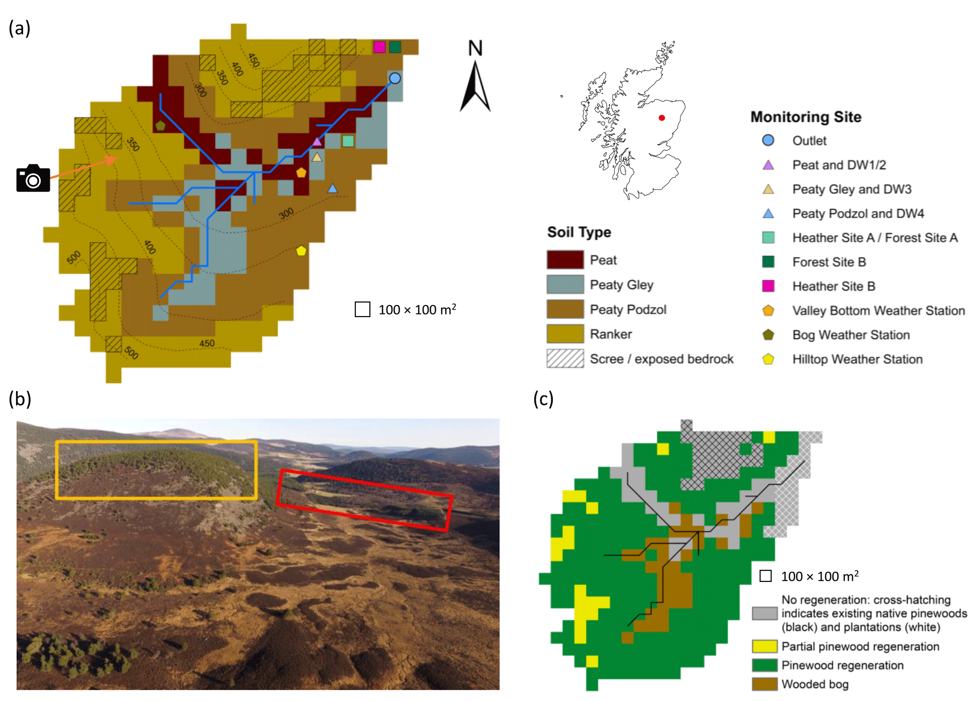
Figure 1 Characteristics of the Bruntland Burn catchment. (a) Map showing the distribution of soil types, monitoring sites (DW is deeper groundwater well) and elevation contours. (b) Aerial view showing the current distribution of vegetation types in the catchment; yellow and red boxes show areas of established natural forest and land managed for plantations, respectively, while the direction of the photo is shown by the arrow in panel (a). (c) Map of regeneration potential (partial pinewood regeneration signifies areas where regeneration was limited to due to presence of scree/exposed bedrock). Photograph in panel (b) by Aaron J. Neill.

Natural Scots pine regeneration is restricted due to grazing from high densities of red deer (Cervus elaphus; 11 to 14.9 deer km⁻²; SNH, 2016) and controlled burning of grouse moorlands. Consequently, tree cover is largely limited to native pinewoods on the relatively inaccessible steep northern hillslope and pine plantations at the catchment outlet (Figs. 1 and 2a). Vegetation otherwise reflects soil type; heather (Calluna vulgaris; Erica tetralix) dominates the peaty podzols and rankers of the hillslopes, while Molinia grassland on the peaty gleys is increasingly outcompeted by Sphagnum spp. on the waterlogged peats of the valley bottom (Fig. 2a). Isolated pine trees are scattered throughout the catchment, with those in the wetter valley bottom exhibiting stunted growth (bog pine in Fig. 2a).

Figure 2 Maps showing the (a) proportional vegetation coverage in the present-day baseline scenario and changes in vegetation cover for the (b) thicket scenario and (c) old open forest scenario. Changes are reported as the regeneration scenario minus baseline scenario. In panel (a), coverages of zero are signified by brown cells.

Mean annual precipitation is 1000 mm, and potential evapotranspiration is 400 mm; the former usually falls in low-intensity events (< 10 mm d⁻¹). Less than 5 % of precipitation is snow, as mean temperatures range between 1 ^∘C in winter and 13 ^∘C in summer. Seepage of fracture flow from bedrock outcrops and shallow sub-surface flow through the rankers predominantly move vertically on reaching the podzols to recharge stores of GW in the underlying drift (Blumstock et al., 2016; Tetzlaff et al., 2014) which sustain baseflow conditions in the stream (Blumstock et al., 2015). The storm response of the BB is non-linear, depending on the dynamic expansion of the riparian saturation area which generates overland flow and hydrological connectivity between the hillslopes and valley bottom (Birkel et al., 2015; Soulsby et al., 2015).

3 Methods

3.1 The EcH₂O-iso model

EcH₂O-iso is a development of the ecohydrological model EcH₂O (Maneta and Silverman, 2013). It consists of three tightly coupled modules simulating the water balance, vertical energy balance and vegetation growth dynamics and an additional fourth module that tracks the stable water isotope composition and ages of hydrological stores and fluxes (Kuppel et al., 2018a). The model domain is defined by a regularly gridded digital elevation model (DEM) that sets local flow directions, and governing equations are solved for fixed time steps using finite differences. Proportional coverages of different vegetation types (based on physiology and structure) and bare soil are specified for each grid cell.

The energy balance is resolved sequentially for the canopy and soil surface. For the canopy, latent (due to transpiration and evaporation of intercepted water) and sensible heat fluxes depend on canopy temperature; this is determined iteratively, such that latent and sensible heat fluxes balance with available net radiation. Interception evaporation is limited by available intercepted water, while a Jarvis-type stomatal conductance model limits transpiration. Transpiration demand is satisfied by root water uptake from three soil layers (L1–3, with L1 being the topmost layer), each with a calibrated depth. Uptake from each layer is proportional to its water content and fraction of roots it contains. The latter is determined by an exponential function describing how the root fraction decreases with depth (Kuppel et al., 2018b). At the soil surface, iteratively determined temperature partitions net radiation and heat advected by rainfall/throughfall into latent heat for snowmelt and soil evaporation from L1, sensible heat exchanges between the soil and atmosphere, and heat into the ground and snowpack. Soil evaporation is limited by the moisture content of L1. In addition to soil, two further hydrological stores are conceptualised, namely canopy interception storage and ponded water. Once interception storage is full, throughfall reaches the ponded water store where it may infiltrate into L1 based on the Green–Ampt model (Mein and Larson, 1973). Vertical redistribution of water occurs via gravitational drainage when volumetric water content in any of the soil layers exceeds field capacity. Drainage rates are proportional to the water content in the layer until they reach effective vertical saturated hydraulic conductivity. Gravitational water in L3 can leak through the bottom model boundary, move laterally as GW simulated via a kinematic wave model or seep into the stream channel. The kinematic wave model assumes that L3 is parallel to the surface, and therefore, flow velocity is proportional to terrain slope and the horizontal effective hydraulic conductivity. The latter, along with an exponential function describing how resistance to flow across the channel–subsurface boundary varies with gravitational water depth, also controls the rate at which seepage to the stream occurs. Water remaining in ponded storage is routed to the next downslope cell as overland flow that can potentially reach the stream within one time step if it is not reinfiltrated along the way. Channel routing is simulated using a kinematic wave model. Isotopes and water ages are tracked assuming complete mixing (Eq. 1 in Smith et al., 2020), with fractionation due to evaporation in L1 simulated via the Craig–Gordon model (Craig and Gordon, 1965; Kuppel et al., 2018a). Vegetation growth dynamics were not simulated in this application; consequently, vegetation characteristics were static for each scenario. For further details of EcH₂O and EcH₂O-iso, see Kuppel et al. (2018a, b), Maneta and Silverman (2013) and Smith et al. (2020).

3.2 Present-day baseline scenario

Catchment soil distribution was based on major Hydrology of Soil Types (HOST) classifications (Fig. 1a; Tetzlaff et al., 2007). The properties of each individual soil type were assumed to be spatially uniform. In total, five vegetation types characterised the present-day baseline scenario, i.e. pre-existing Scots pine, heather (also used to represent other understorey shrubs such as bilberry), Molinia grass, Sphagnum and bog pine (Table 1). Lidar-based estimates of canopy cover were used to derive proportional tree coverages in each cell (see Kuppel et al., 2018b). Trees on the podzols/rankers (plus those in plantations) and on the wetter peat/peaty gleys were designated as pre-existing pine and bog pine, respectively (Fig. 2a). This permitted explicit representation of stunted growth in the latter due to waterlogging (McHaffie et al., 2002). The extents of remaining vegetation types (Table 1; Fig. 2a) were derived from the soil distribution, field mapping and aerial imagery (Kuppel et al., 2018b; Tetzlaff et al., 2007). To account for scree and exposed bedrock (Fig. 1a), some rankers on the western and northern hillslopes were set with bare earth coverages of 80 % and up to 95 % of the treeless surface, respectively. All vegetation heights in the baseline scenario were based on local knowledge (Table 1).

Table 1 Vegetation types in each scenario organised by soil type. All vegetation types are shown for the baseline scenario while only those in areas of pinewood regeneration on podzols/rankers or wooded bog on peaty gleys are given for the regeneration scenarios (see Fig. 1c). In areas where regeneration is not possible, vegetation characteristics remain as they were in the baseline scenario. The total coverage of all vegetation types plus bare earth sum to 100 % within each cell of a given soil type. Leaf area index (LAI) scale factors convert calibrated values of LAI for pre-existing pine to LAI values for thicket, old open or bog pine.

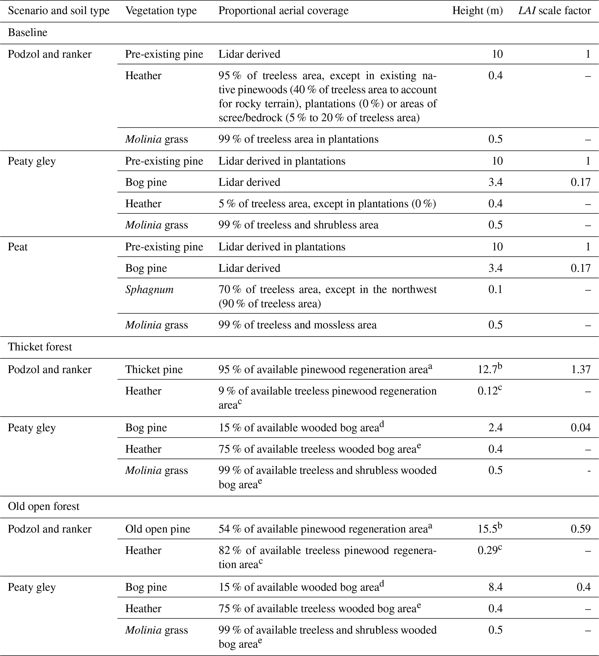
Note: ^a Based on plan drawings of thicket (type 25) and old open forest (type 3) as seen in Fig. 3 of Summers et al. (1997). ^b Median height of aged trees from thicket and old open woodland as seen in Table 2 of Summers et al. (2008). ^c Sum of shrub cover or cover-weighted average height of shrubs for thicket and old open pines in Table 1 of Parlane et al. (2006). ^d Based on pine cover in uncut wooded bogs reported by McHaffie et al. (2002). ^e Based on field descriptions of Steven and Carlisle (1959).

3.3 Baseline calibration

The baseline scenario was simulated from 21 February 2013 to 8 August 2016 on a 100 m × 100 m grid with a daily time step. Model forcing data are detailed in the Supplement (Table S1). A total of 6 years of looped data were used to spin-up the model for calibration, while 30 years were used for post-calibration runs to stabilise water ages (see Kuppel et al., 2020). Calibration followed a Morris sensitivity analysis (Morris, 1991; Sohier et al., 2014) to identify sensitive parameters (Table S2). For efficiency, it was assumed that pre-existing pine and bog pine vegetation types could take the same parameter values, except for LAI (italics signify model parameter names); thus, only four sets of vegetation parameters required calibration. Overall, 90 parameters (10×4 for soil, 12×4 for vegetation and 2 for stream channel) were calibrated. The parameter space was sampled by conducting 100 000 Monte Carlo simulations. Parameter values were drawn from initial ranges informed by Kuppel et al. (2018b) and additional literature reviews (Table S2). The LAI of bog pine was related to the sampled LAI of pre-existing pine via a scale factor accounting for relative differences in canopy architecture. The scale factor (0.17) was derived by dividing an empirical estimate of LAI for bog pine by a local measurement of LAI for pre-existing Scots pine (Wang et al., 2018). The former was obtained by first estimating the fraction of above-canopy irradiance passing through the canopy as a function of tree height (3.4 m) and density (275 trees ha⁻¹; Summers et al., 1997) via the equation of Parlane et al. (2006). This was then used in Beer's law with a light extinction coefficient of 0.5 (White et al., 2000) to determine LAI.

Diverse ecohydrological and isotope data sets were available at the BB catchment for model calibration (Table 2). Protocols used to collect and process these data are detailed in Kuppel et al. (2018a, b). In most cases, model outputs were directly compared against relevant observed data sets. Simulated soil variables (volumetric water content and bulk water isotopes) were exceptions; these are output for each soil layer and, therefore, do not directly correspond to depth-specific observations (see Beven, 2006). To accommodate this, simulated volumetric water content time series for L1 and L2 were compared to observations made at the depth closest to the mid-point of each layer. Meanwhile, simulated soil water isotopes in L1 and L2 were compared with the average of observations made within the soil profile encompassed by each respective layer. Consequently, observations compared to simulated outputs from L1 and L2 could vary, depending on soil depth parameterisation.

Table 2 Data sets used in the calibration of EcH₂O-iso and their temporal coverage (full study period is 21 February 2013 to 8 August 2016). Performance metrics used to quantify the skill of the model in simulating each data set and the range of values achieved by the 30 behavioural model runs are also given.

Note: ^a MAE is the mean absolute error, and RMSE is the root mean squared error. ^b Range across first two soil layers of EcH₂O-iso. ^c Tr is transpiration, and ET is evapotranspiration.

Model skill in simulating the dynamics of ecohydrological and isotopic observations was quantified using the performance metrics in Table 2. Mean absolute error was used for discharge to avoid over-emphasis of high flows that can occur when using metrics based on mean squared errors (Krause et al., 2005). It was further used for all isotope simulations given the limited variability in observations and the daily time step of the model (see Gupta et al., 2009; Schaefli and Gupta, 2007). Root mean squared error was otherwise used as this is recommended if no information is available on error distributions (Chai and Draxler, 2004; Kuppel et al., 2018b). To determine behavioural parameter sets, model runs were first selected that simulated saturation areas < 60 % of total catchment area for at least 90 % of the simulation period; this reflected mapping and modelling of the extent of saturation in the BB catchment (Birkel et al., 2010). Performance metrics for each calibration data set were then ranked across all runs that satisfied this constraint. Runs were finally ordered by their worst-performing metric, with the best 30 runs being retained as behavioural; this balanced the need to illustrate uncertainty in model outputs with the increased computational demand of producing spatial outputs required post-calibration.

3.4 Regeneration scenarios

Extensive work characterising the structure of native pine stands at Abernethy Forest in the Cairngorms National Park (Parlane et al., 2006; Summers, 2018; Summers et al., 1997, 2008) was used to select two stages of forest regeneration for simulation. For context, Fig. S1 in the Supplement summarises the general sequence of natural pinewood regeneration. The thicket stage has the highest tree densities and near-complete canopy closure; consequently, this stage was selected because it will likely have the most substantial impact on water partitioning and catchment hydrology. Trees are ∼ 40 years old, while understorey development is limited. Old open forest was chosen as the second stage and represents a possible realisation of old-growth forest. This stage may be somewhat semi-natural, with a canopy that is perhaps too open as a consequence of past silvicultural practices and upland grazing (Summers et al., 2008). Consequently, regeneration of such a forest would require a rewilding trajectory that seeks to restore natural regeneration while also employing passive management to preserve characteristics of a landscape that reflects elements of Scottish cultural heritage and/or the habitats provided by such a semi-natural environment (see Deary and Warren, 2017). Nonetheless, it was chosen as a possible lowest impact stage of late forest development and, thus, offers an extreme contrast to the thicket scenario. Trees are tall, old (∼ 150 years) and sparsely distributed, with an understorey of well-developed shrubs.

The proportional coverage and characteristics of vegetation at each stage of forest regeneration are given in Table 1. Native pinewoods, consisting of thicket/old open pine and a heather understorey, were assumed to fully regenerate on podzols and rankers (Fig. 1c), reflecting the preference of pine for freely draining minerogenic soils (Mason et al., 2004). The available regeneration area was limited in ranker cells containing scree or exposed bedrock such that the bare earth fraction remained constant across scenarios, while regeneration did not occur on managed land at the catchment outlet or in pre-existing areas of native pinewood on the northern hillslope (Fig. 1c). A wooded bog consisting of stunted bog pine, heather and Molinia grass, was simulated on the wetter peaty gleys (McHaffie et al., 2002; Steven and Carlisle, 1959; Summers et al., 1997), while no regeneration was possible on the waterlogged peat (Fig. 1c). Spatial changes in vegetation cover for each regeneration scenario relative to the baseline are shown in Fig. 2b–c. Scale factors relating calibrated values of LAI for pre-existing pine to the LAI of thicket, old open and bog pine were calculated as described in Sect. 3.3. For thicket/old open pine, measured fractions of the above-canopy irradiance passing through the canopy were available from Parlane et al. (2006). Estimates for bog pine were again made via the equation of Parlane et al. (2006). The heights of bog pine in each scenario were estimated by first calculating a stunted growth rate (∼ 0.06 m yr⁻¹) by dividing the height of present-day bog pine by an assumed age of 60 years. This was multiplied by the age of pines in the thicket (40 years) and old open (150 years) forests to give bog pine heights of 2.4 and 8.4 m for each scenario, respectively. These values are broadly consistent with height measurements made by Summers et al. (2008) on bog pine trees with an interquartile age range between 72 and 143 years.

Simulations were driven by the 30 behavioural parameter sets obtained from the baseline calibration and undertaken for the same time period (21 February 2013 to 8 August 2016) with 30 years of spin-up. As previously stated, soil properties remained unchanged in the regeneration scenarios. Additionally, the vertical root distribution parameter was consistent amongst pine vegetation types as after the sapling stage; the most significant changes to Scots pine rooting characteristics are expressed in the horizontal rather than vertical direction (Laitakari, 1927; Makkonen and Helmisaari, 2001). Potential effects of such changes on the vertical root distribution would likely already be captured by the sampling range of this parameter for pre-existing pine (Table S2).

3.5 Change analysis

To contextualise changes to water flux partitioning, simulated maximum root zone and interception storage capacities were quantified for each scenario. For each vegetation type in a given grid cell, root zone storage capacity was defined as the sum of maximum plant-available volumetric water content in each layer weighted by root fraction, multiplied by the coverage-weighted average rooting depth of all vegetation types in the cell. A coverage-weighted sum across all present vegetation types then yielded the total root zone storage capacity for the cell. The total interception storage capacity of each cell was similarly calculated, with the interception storage capacity of each vegetation type obtained by multiplying the parameters LAI and maximum canopy storage (Table S2). Values of root zone and interception storage capacity at the catchment scale were then derived.

Catchment-scale flux partitioning was assessed by quantifying seasonally averaged flux totals for simulated discharge at the outlet, GW recharge, soil and interception evaporation, and transpiration. Seasons were defined as April to September (active season) and October to March (dormant season), broadly corresponding to biologically active and dormant periods in northeastern Scotland, respectively (Dawson et al., 2008). Seasonal volume-weighted average water ages were also calculated for selected stores and fluxes. Daily time series of discharge, stream isotopic composition and water age provided a spatially integrated insight into how regeneration affected modelled catchment hydrology at a higher temporal resolution. To better understand spatial drivers of changes to catchment-scale flux partitioning, differences in seasonal daily average blue and green fluxes between each scenario and the baseline were spatially disaggregated.

To assess how regeneration impacts hydrological source areas and runoff generation, the spatial extent of hydrological connectivity was quantified under contrasting flow conditions. A cell was considered hydrologically connected if overland flow (OLF) was simulated for the cell and all downslope cells along the flow path to the stream. No minimum threshold of OLF was imposed for a cell to be considered connected (see Turnbull and Wainwright, 2019), as EcH₂O-iso simulates re-infiltration along a given flow path which can prevent upslope cells producing OLF from connecting to the stream (Maneta and Silverman, 2013). Flow path lengths for connected cells were calculated by accumulating the straight line or diagonal lengths (dependent on local flow direction) of all cells along the flow path (see Turnbull and Wainwright, 2019). A total of four different flow conditions were considered for the connectivity analysis, with each assessed using OLF simulations from a representative date, as follows: (1) summer baseflows (22 July 2013), (2) small to moderate events during summer and autumn/winter rewetting (15 September 2014), (3) larger summer events (20 July 2016) and (4) large winter events (30 December 2015).

4 Results

4.1 Baseline calibration

Figure 3 summarises the skill of the model in simulating blue and green fluxes, isotope dynamics and net radiation at selected monitoring locations (remaining simulations shown in Figs. S2–S5). Performance metrics and calibrated parameter ranges are given in Tables 2 and S2, respectively. Stream discharge was generally well simulated, with only occasional under-prediction of baseflows (e.g. summer 2016) and the most extreme events. At most sites, modelled volumetric water content in L1 and L2 was bracketed by the range observed across the soil profile, although simulations were sometimes less dynamic than observations, and root mean squared errors could be large. However, this likely reflects the commensurability issues highlighted in Sect. 3.3 (also relevant for soil water isotopes), and the fact that Heather A and Forest A fell within the same model cell. The model was generally successful in reproducing dynamics of stream water, soil water and groundwater isotopes, implying internal catchment functioning was reasonably well captured. Stream isotopes were sometimes over-enriched, suggesting slightly high soil evaporation; however, the variability was generally well captured. Larger deviations during events likely reflect structural limitations of the model (e.g. the ability of OLF to traverse the catchment within one time step). Excessive evaporation was not apparent from simulated soil water isotopes, although averaging over L1 and L2 could obscure the effects of evaporative fractionation in the former. The model had skill in simulating ET and forest transpiration. However, underestimation of heather transpiration may indicate excessive radiative energy being used for evaporation. Seasonality in net radiation was well simulated, though shorter-term variability was under-estimated in summer.

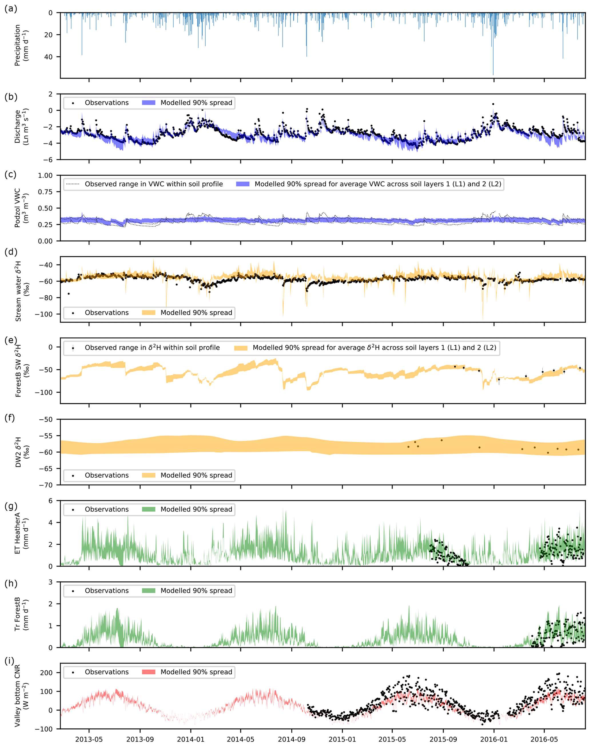
Figure 3 Time series of (a) precipitation and of the observed and simulated (b) natural logarithm (Ln) of stream discharge. (c) Volumetric water content (VWC) at the peaty podzol site. (d) Stream δ²H composition. (e) Bulk soil water (SW) δ²H under Forest B. (f) Groundwater δ²H at deeper well 2 (DW2). (g) Total evapotranspiration (ET) for Heather A. (h) Transpiration (Tr) for Forest B. (i) Net radiation (CNR) at the valley bottom weather station. The 90 % spread of simulations are from the 30 behavioural model runs.

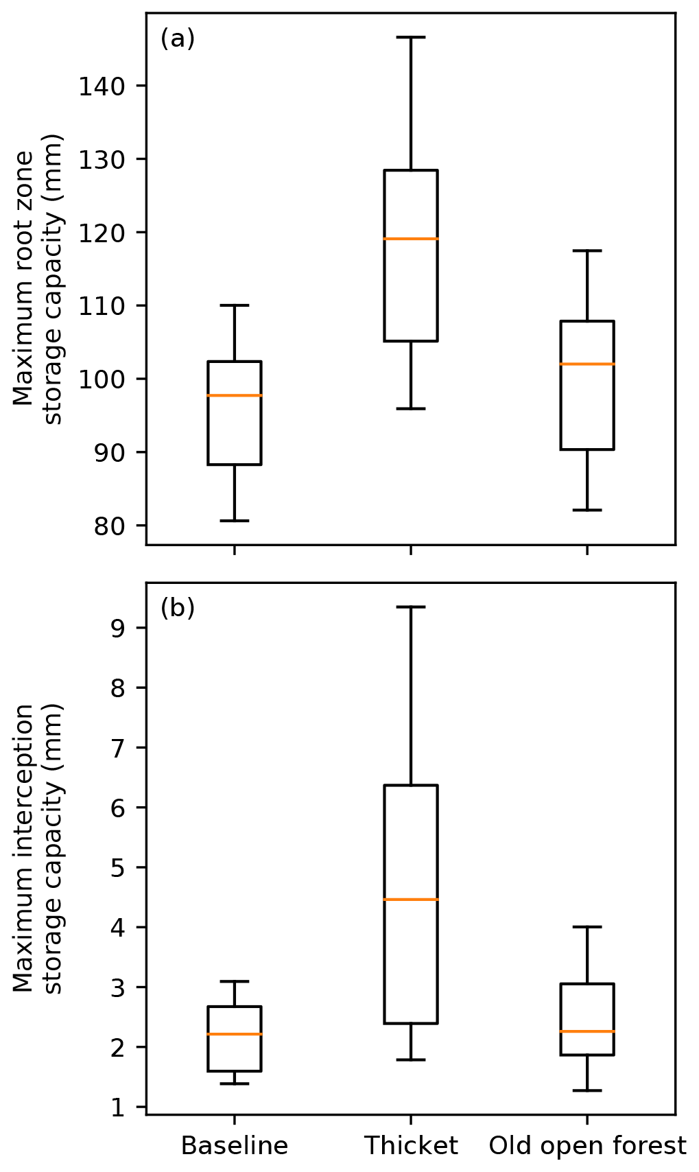
Figure 4 Box plots showing maximum (a) root zone storage capacity and (b) interception storage capacity, for the baseline and forest regeneration scenarios. The median is shown by the orange line, while the box extends from the lower to upper quartiles. The 5th and 95th percentiles are given by the tails.

4.2 Impact of regeneration on water storage capacity

Figure 4 summarises simulated root zone and interception storage capacities for each scenario. Median root zone storage capacity increased by 21 mm in the thicket forest scenario, reflecting replacement of heather by thicket pine (Fig. 2b) with deeper roots (Table S2) that increase access to water stored in L2 and L3. Small increases in root zone storage capacity were simulated for the old open forest scenario, albeit with greater overlap with the baseline, likely reflecting the more balanced composition between pine and heather (Fig. 2c). This, along with greater proportional coverage of bare earth (Fig. 2c), may also explain overlap of interception storage capacity between the old open forest and baseline scenarios. The greater coverage of thicket pine (Fig. 2b) with a dense canopy substantially increased interception storage capacity for the thicket forest scenario.

4.3 Changes to catchment-scale water flux partitioning

Figure 5 shows how impacts of modelled regeneration integrated to affect the simulated quantity and isotopic composition of streamflow. Discharge was most notably reduced in the thicket scenario. Proportional reductions in discharge (as revealed by considering its natural logarithm) appeared to show an annual cycle, generally increasing in magnitude through the summer months and into the autumn/winter rewetting period before being reset by a sufficiently large winter event that resulted in more limited divergence of subsequent winter and spring flows. Consequently, low to moderate flows during the summer and autumn/winter rewetting period were most affected in the thicket scenario, while higher flows remained relatively consistent. For the old open forest scenario, discharge was similar to the baseline. For both regeneration scenarios, simulated stream isotope dynamics were comparable to the baseline; however, stream water could sometimes be slightly more depleted in summer for the thicket scenario, indicating reduced soil evaporation.

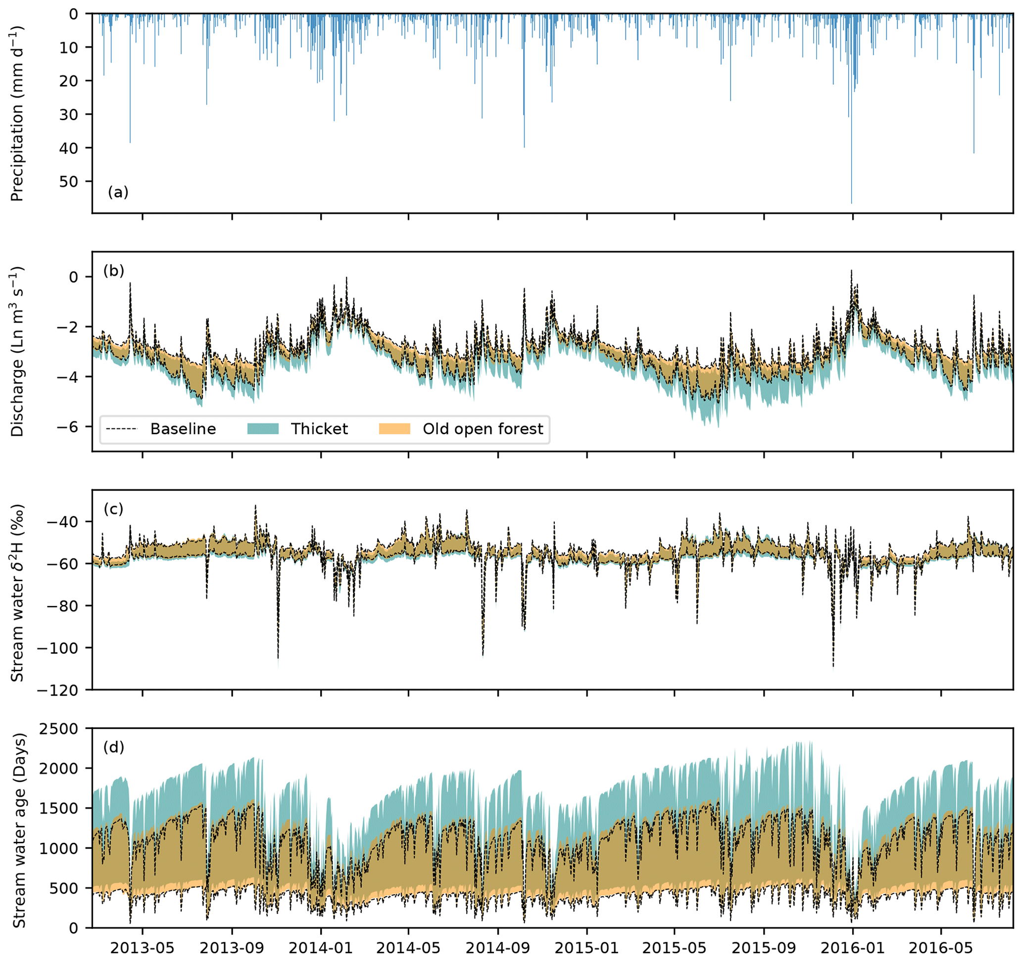
Figure 5 Time series of the (a) observed precipitation and the simulated (b) natural logarithm (Ln) of stream discharge. (c)  Stream water δ²H composition. (d) Stream water age. In panels (b) to (d), the area between the two black lines represents the 90 % spread of behavioural simulations for the baseline scenario, while the shaded areas show the same for the thicket and old open forest scenarios. Areas of darker, gold-coloured shading occur where simulations for the two regeneration scenarios overlap.

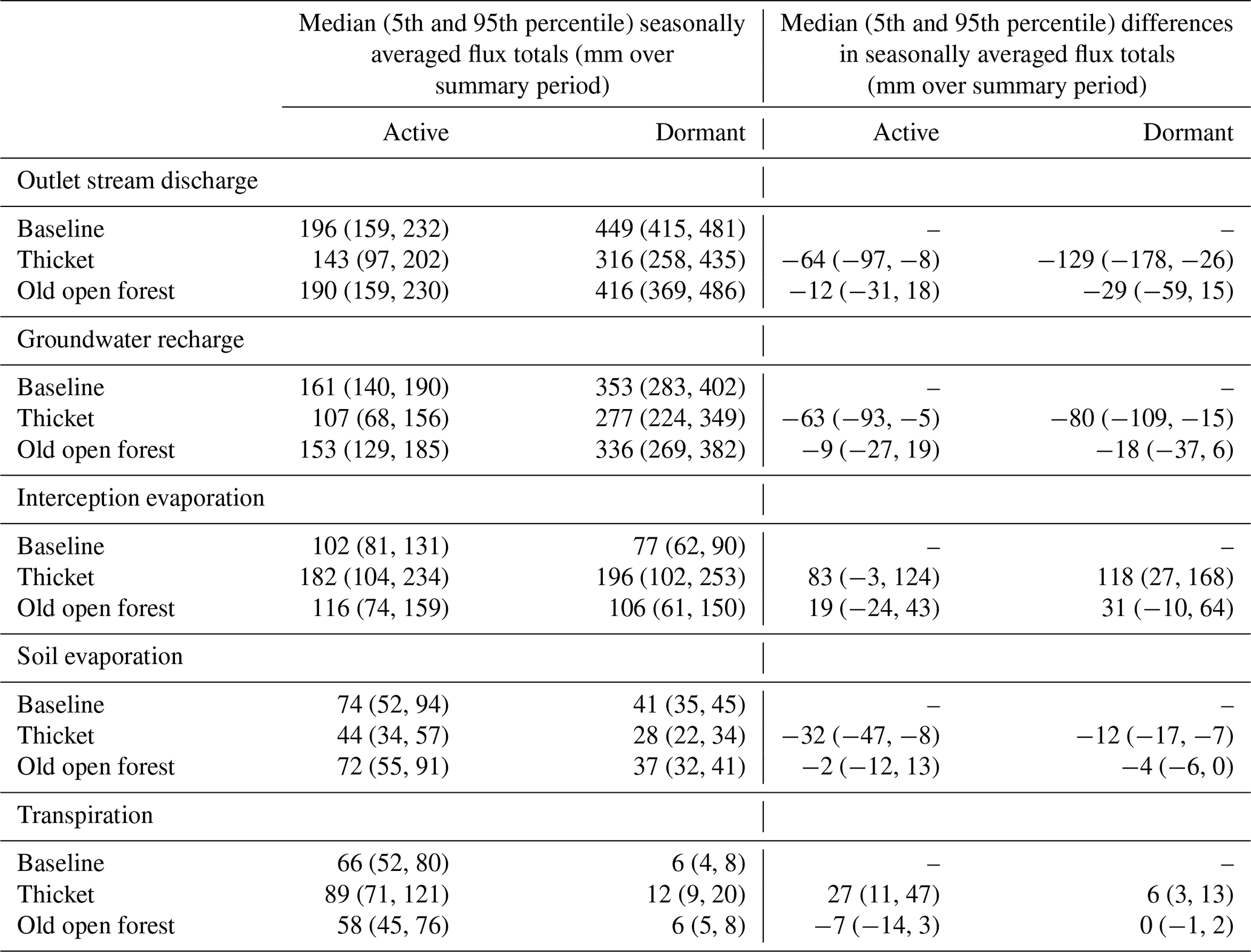
Table 3 summarises the changes to seasonally averaged water flux totals. Overall, behavioural models consistently simulated a decrease in seasonally averaged discharge for the thicket scenario. This resulted from increased interception evaporation and transpiration and decreased GW recharge. Recharge was most reduced for the dormant season, concurrent with the greatest increase in interception evaporation. Soil evaporation was lower for the thicket scenario, likely reflecting limits imposed by lower soil moisture due to greater interception evaporation and transpiration losses, and reduced penetration of radiation through the thicket canopy. Differences in seasonally averaged fluxes were much smaller between the old open forest and baseline, resulting in the median and 5th and 95th percentile seasonally averaged flux totals generally being similar for the two scenarios. However, there was a repartitioning of water between increased interception evaporation and reduced GW recharge for the dormant season that contributed to an ∼ 30 mm decrease in the median seasonally averaged discharge total.

Table 3 Seasonally averaged water flux totals and differences in seasonally averaged totals. Totals and differences were calculated for each behavioural run individually and summarised by the median and 5th and 95th percentile (in parentheses) values across all behavioural runs. Differences are reported as the regeneration scenario minus baseline and help to indicate whether the simulated direction of change in each flux was consistent among behavioural models. Active and dormant seasons cover April to September and October to March, respectively.

4.4 Spatiotemporal dynamics of baseline flux partitioning

Figure 6 summarises the spatial dynamics of median seasonal daily average blue and green fluxes for the baseline scenario. Simulated OLF was more limited for the active season. The largest fluxes were simulated for the peats and peaty gleys, with some OLF also being generated by the ranker soils on the hillslopes. The latter is interpreted as representing the rapid near-surface flows in the shallow rankers that are driven by the emergence of bedrock fracture flow at slope breaks. OLF fluxes were greater and had similar spatial patterns for the dormant season, with additional fluxes generated from the podzols on lower hillslopes in the north and south. Vertical movement of water (infiltration and GW recharge) was greatest in the dormant season and mostly occurred on the podzols; the largest fluxes were simulated at the boundaries between the podzols and rankers reflecting lateral flows from upslope moving vertically in deeper soils. Water was then simulated to move downslope as GW to sustain saturation in the valley bottom, as evidenced by high exfiltration fluxes especially in the dormant season.

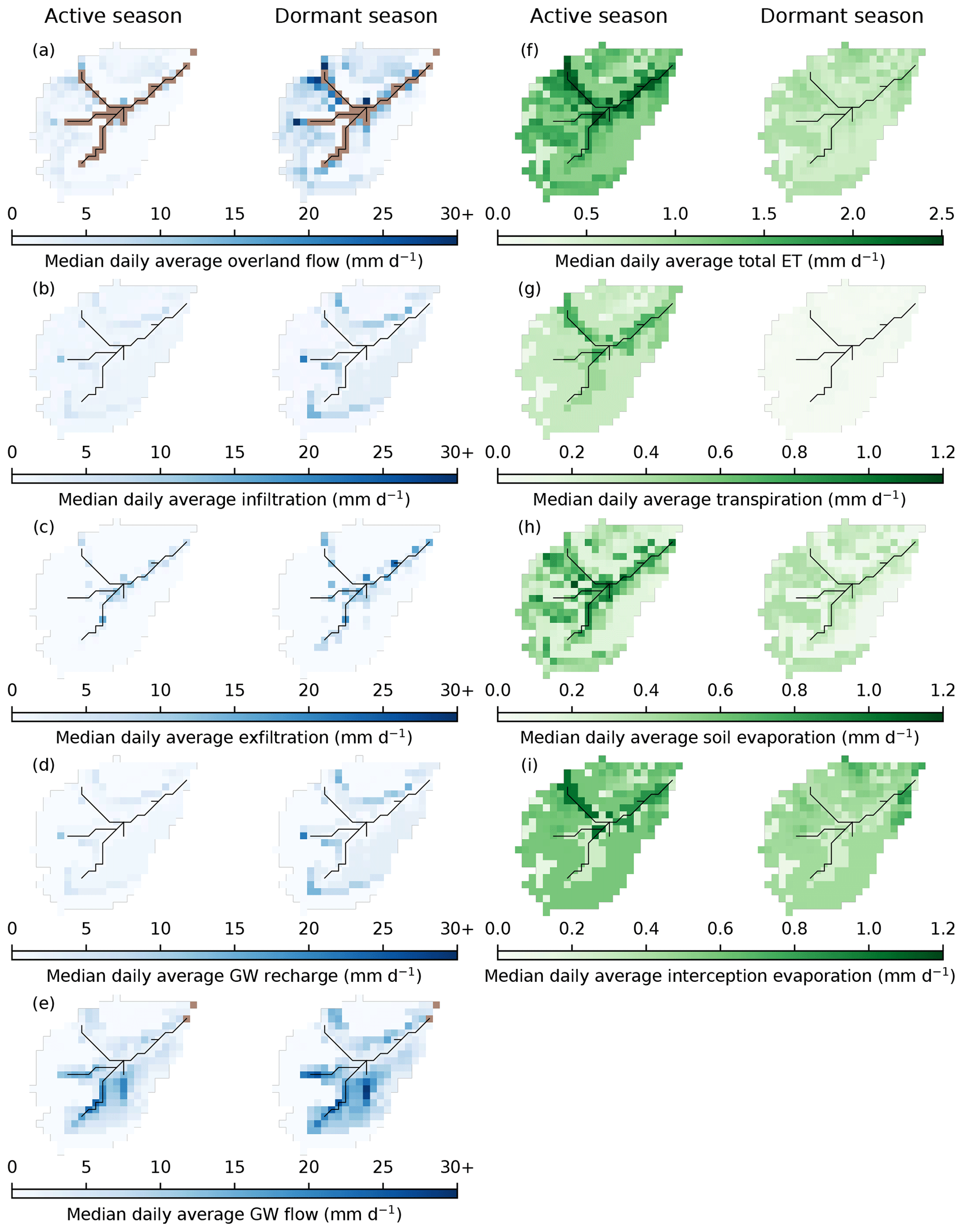
Figure 6 Maps showing median daily average fluxes of the baseline scenario for the active (April to September) and dormant (October to March) seasons. (a) Cell-to-cell overland flow. (b) Infiltration into the first soil layer (L1). (c) Exfiltration to the surface. (d) Groundwater (GW) recharge. (e) Cell-to-cell lateral GW flow. (f) Total evapotranspiration (ET). (g) Transpiration. (h) Soil evaporation. (i) Interception evaporation. Brown cells in panels (a) and (e) are cells for which EcH₂O-iso does not simulate cell-to-cell overland (channel and outlet cells) and lateral GW flows (outlet cells). Colour bar for blue fluxes is truncated at upper limit to aid in the presentation of spatial patterns (largest flux is 38.9 mm d⁻¹ for overland flow). Note that total ET is on a different scale to the other green fluxes.

Daily average fluxes of ET were simulated as being greatest for the active season, particularly in the valley bottom (Fig. 6). This was facilitated by the wet peat and peaty gleys maintaining transpiration and soil evaporation and by evaporation of water intercepted by the Sphagnum canopy. Dominance of vertical sub-surface fluxes limited transpiration and, particularly, soil evaporation from the podzols, reducing total ET fluxes. For the dormant season, spatial patterns in total ET were less distinct, reflecting reduced soil and interception evaporation in the valley bottom and the fact that daily transpiration fluxes were essentially zero. A notable pattern was that total ET was particularly elevated where there was substantial pre-existing pine (Figs. 2a and 6f) due to sustained interception evaporation.

4.5 Spatiotemporal disaggregation of regeneration effects on flux partitioning

Median differences in seasonal daily average blue fluxes were most dramatic for the thicket scenario (Fig. 7). For both the active and dormant seasons, similar spatial patterns were simulated, although differences tended to be greater for the latter. More limited OLF generation by the rankers led to similar magnitude reductions in daily average infiltration and GW recharge on the podzols. Consequently, downslope movement of GW also decreased in both seasons. This contributed to a drying out of the valley bottom (especially in the dormant season), even though local regeneration was limited (Fig. 2b). Daily average OLF fluxes were simulated to decrease around the fringes of the stream for both seasons. The largest decreases occurred in the northwest of the catchment as a direct consequence of reduced OLF from upslope. Elsewhere, OLF reductions strongly reflected the reductions in upslope GW subsidies as evidenced by consistently decreased exfiltration fluxes and increased infiltration of incoming precipitation in the valley bottom for the dormant season to replenish drier soil and GW stores.

Figure 7 Maps showing the median difference in daily average blue fluxes for the active (April to September) and dormant (October to March) seasons. (a) Cell-to-cell overland flow. (b) Infiltration into the first soil layer (L1). (c) Exfiltration to the surface. (d) Groundwater (GW) recharge. (e) Cell-to-cell lateral GW flow. Differences are reported as the regeneration scenario minus baseline scenario. Brown cells in panels (a) and (e) are cells for which EcH₂O-iso does not simulate cell-to-cell overland (channel and outlet cells) and lateral GW flows (outlet cells). Colour bar is truncated at the lower limit to aid in the presentation of spatial patterns (largest negative difference is −9.7 mm d⁻¹ for overland flow).

Similar spatial dynamics were simulated for the old open forest scenario; however, median differences in seasonal daily average fluxes were much reduced (Fig. 7). It is also noteworthy that, even in the dormant season, the valley bottom dried out less than in the thicket scenario; daily average GW flows through the podzols were only simulated to decrease by < 1.5 mm d⁻¹, while no increases in infiltration or GW recharge were simulated in the valley bottom.

Differences in seasonal daily average green fluxes were also more apparent in the thicket scenario (Fig. 8). Daily average ET from the podzols and rankers was simulated to increase throughout the year. For the active season, this resulted from greater transpiration and, predominantly, interception evaporation, reflecting the increased coverage of thicket pine (Fig. 2b). Reduced penetration of radiative energy through the thicket canopy, and limits imposed by greater water losses to transpiration and interception evaporation, decreased simulated daily average soil evaporation. For the dormant season, increased ET was more driven by greater interception evaporation. ET from the wooded bog was similar to the baseline. This was due to decreased transpiration from reduced cover of potentially deep-rooted (Aerts et al., 1992; Taylor et al., 2001) Molinia grass (Fig. 2b) being compensated by increases in soil and, particularly, interception evaporation. Daily average ET for the active season decreased in some areas of peat despite no regeneration having taken place. This would be consistent with drying of the valley bottom limiting summer transpiration.

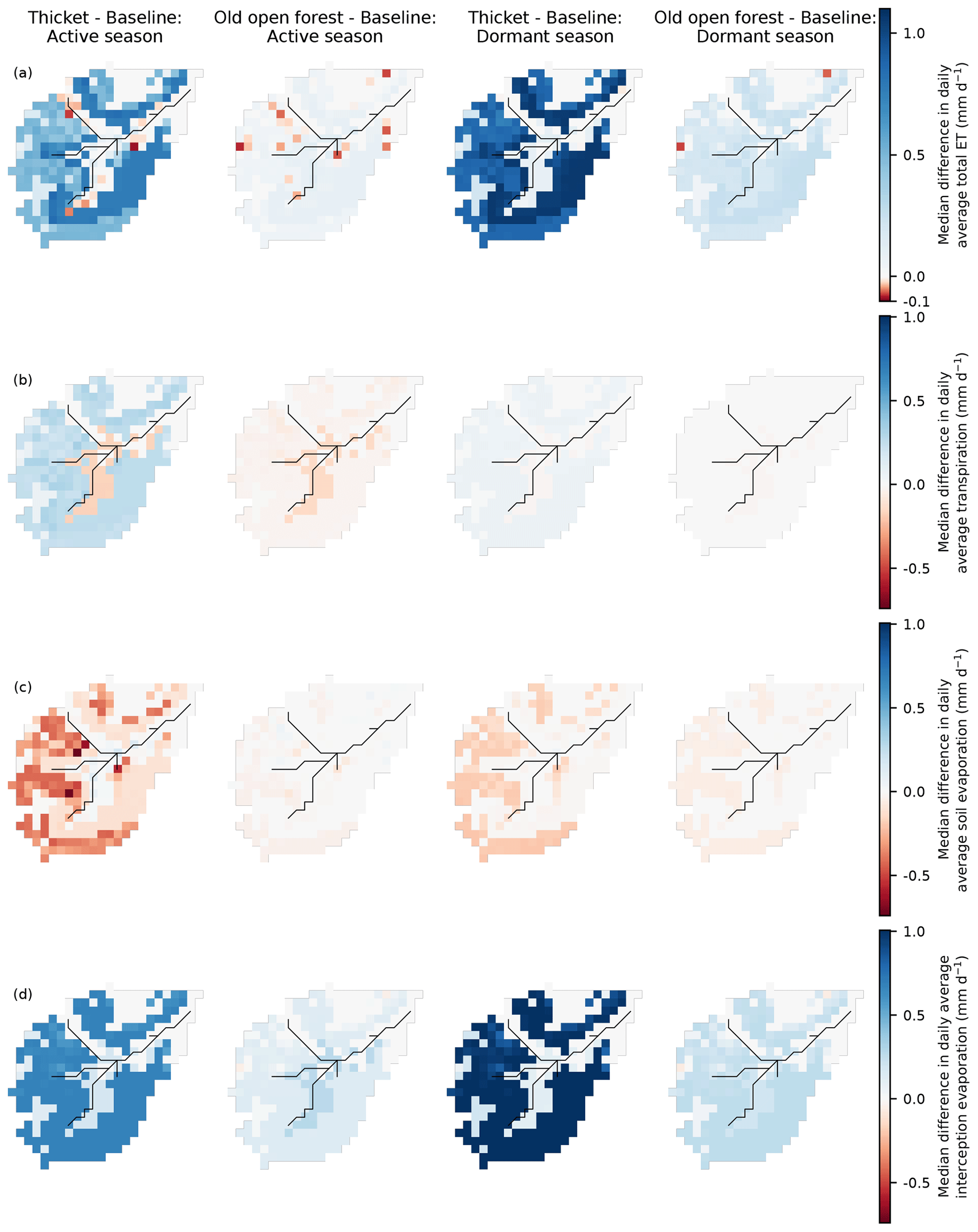
Figure 8 Maps showing the median difference in daily average green fluxes for the active (April to September) and dormant (October to March) seasons. (a) Total evapotranspiration (ET). (b) Transpiration. (c) Soil evaporation. (d) Interception evaporation. Differences are reported as regeneration scenario minus baseline scenario. Note that total ET is on a different scale to the other fluxes.

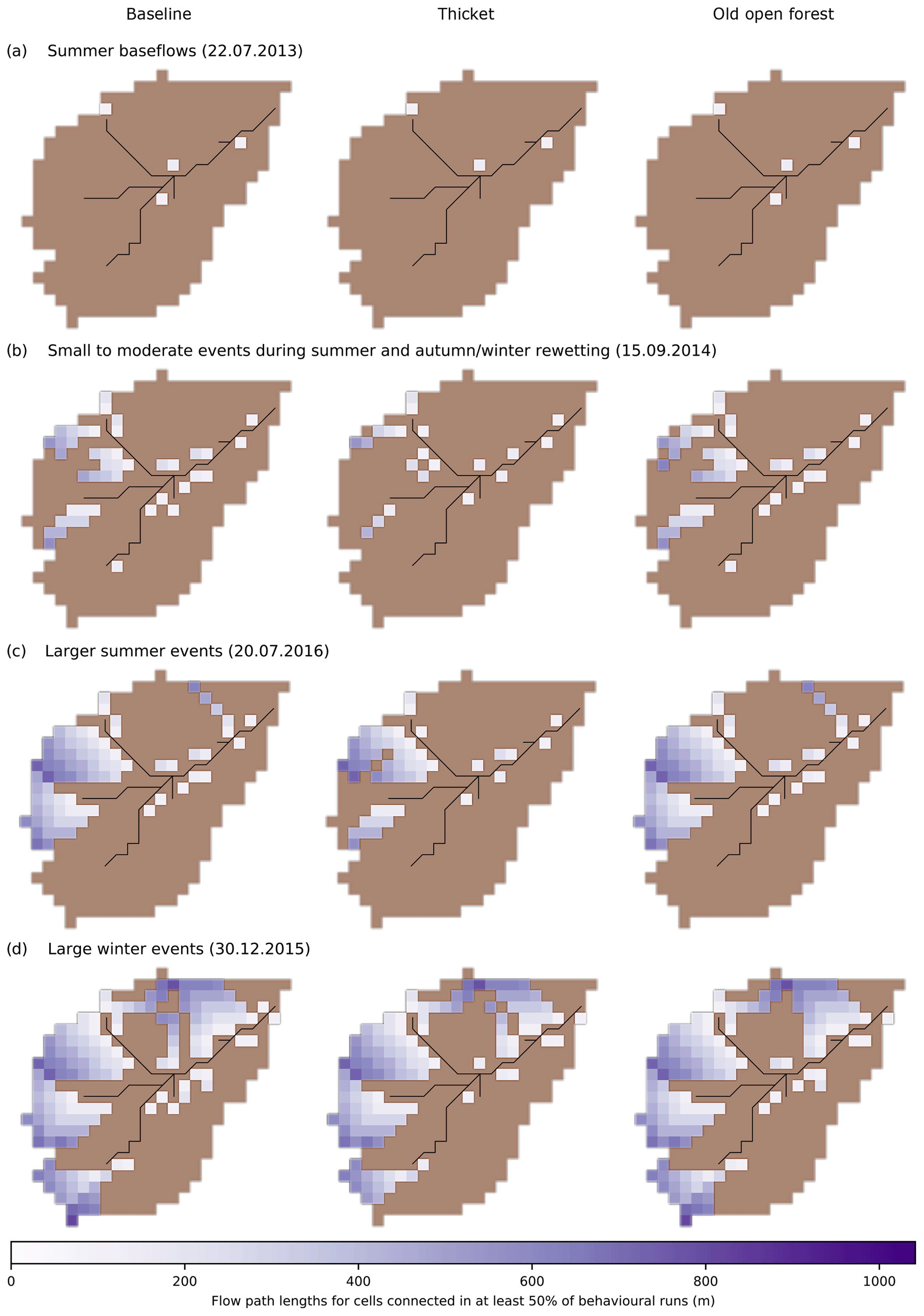
Figure 9 Spatial patterns of hydrological connectivity simulated in at least 50 % of behavioural model runs for dates representative of (a) summer baseflows, (b) small to moderate events during summer and autumn/winter rewetting, (c) larger summer events and (d) large winter events. Disconnected cells are shown in brown.

Differences in simulated ET were much more subdued for the old open forest scenario (Fig. 8). For the active season, soil evaporation on the rankers and podzols, in particular, remained similar to the baseline, while transpiration showed a more consistent slight decrease. This offset greater losses to interception evaporation so that only small increases in total ET were simulated. Very small ET decreases mostly reflected the replacement of larger clusters of pre-existing pine with old open forest (Fig. 2c) leading to reduced transpiration. A larger increase in interception evaporation from the old open forest drove the increases in ET from the podzols and rankers for the dormant season.

4.6 Effects of regeneration on ages of blue and green water

Streamflow, lateral GW outflows and soil water/evaporation were near-consistently simulated to have older average ages in the thicket scenario relative to the baseline (Table 4); however, change magnitudes were often less than the width of simulation uncertainty bounds leading to overlap in flux ages. Simulated daily dynamics revealed that stream water ages for the thicket scenario could be much older for low to moderate flows, although uncertainty bounds were again wide (Fig. 5d). Relatively young stream water ages persisted in larger events. Transpiration fluxes were the only ones to indicate a possible slight preference for younger water through a reduction in 95th percentile average ages (Table 4). For old open forest, age characteristics were generally restored to those simulated for the baseline.

Table 4 Seasonally averaged water flux ages and differences in seasonally averaged ages. Averages and differences were calculated for each behavioural run individually and summarised by the median and 5th and 95th percentile (in parentheses) values across all behavioural runs. Differences are reported as regeneration scenario minus baseline and help indicate whether the simulated direction of change in the average age of each flux was consistent amongst behavioural models. Active and dormant seasons cover April to September and October to March, respectively.

4.7 Changes to hydrological connectivity

For the considered flow conditions, Fig. 9 summarises spatial patterns of hydrological connectivity that were simulated by at least 50 % of the behavioural model runs. Baseline connectivity during summer baseflows was only established for a limited number of cells close to the stream; for 22 July 2013 only ∼ 1 % of cells were connected due to particularly dry summer conditions at this time (Fig. 9a). In the thicket scenario, the spatial extent of connectivity became even more limited, though saturation in the valley bottom was maintained. Regeneration of old open forest did not substantially affect connectivity dynamics; indeed, this was the case for all flow conditions considered. The catchment had a wetter baseline state for small to moderate summer and autumn/winter rewetting events, with 14 % of cells being connected on 15 September 2014 (Fig. 9b). This reflected greater connectivity in the valley bottom and the establishment of longer flow paths (up to 600 m) in the west of the catchment. These flow paths tended to become shorter in the thicket scenario; along with slightly less connectivity in the valley bottom, this caused a 52 % reduction in cells that were connected to the stream. Stronger connectivity and longer flow paths (up to 800 m) in the west of the catchment and establishment of a long flow path down the northern hillslope led to 25 % of cells being connected in the representative larger summer event on 20 July 2016 (Fig. 9c). While some cells with longer flow paths did disconnect in the thicket scenario, the largest reductions in connectivity resulted from the disconnection of cells with more moderate flow path lengths (up to 600 m) in the west of the catchment. Despite this, however, large connected areas were maintained in both the west of the catchment and valley bottom, leading to a 36 % reduction in connectivity overall. Large winter events showed the greatest baseline connectivity, with 48 % of cells connected to the stream on 30 December 2015 (Fig. 9d). This reflected greater establishment of connectivity on the northern hillslope and in the southwest headwater that also increased the number of connected cells with moderate to long (400 to 1000 m) flow path lengths. Spatial patterns of connectivity were similar overall in the thicket scenario, with the main notable changes being reduced connectivity in the southwest headwaters and disconnection of specific flow paths on the northern hillslopes due to more limited OLF generation from some riparian cells (e.g. around the headwater confluences – Fig. 7a). These changes led to just a 16 % reduction in the total number of cells connected to the stream.

5 Discussion

5.1 Simulated effects of natural forest regeneration on blue and green water partitioning

Previous studies investigating the hydrological consequences of changes in forest cover have often sought to understand how conversion and management of land for commercial forestry affects aggregated metrics of catchment hydrological functioning (Ellison et al., 2017; Filoso et al., 2017), especially so in the UK context (Marc and Robinson, 2007). Consequently, findings may not be transferable to the case of passively managed natural forest regeneration that is the goal of rewilding efforts in degraded landscapes such as the Scottish Highlands (zu Ermgassen et al., 2018). Therefore, using the EcH₂O-iso model, we investigated the ecohydrological consequences of natural pinewood regeneration for the BB catchment in Scotland by comparing simulated present-day baseline conditions with two land cover change scenarios representing different stages of forest regeneration (thicket and old open forest).

The overall skill of the model in capturing the dynamics of diverse ecohydrological and isotope data sets (Table 2; Fig. 3) helped provide confidence in its ability to simulate plausible realisations of catchment functioning. However, despite the rich calibration data set, larger uncertainties persisted in some model outputs (e.g. water ages; Fig. 5d). This likely reflected a combination of several factors, including the extent to which available data can constrain specific details of individual processes simulated by complex models alongside more general features of catchment functioning (e.g. surface water vs. GW dominated; Holmes et al., 2020; Neill et al., 2020), limitations in the information content of certain data sets (e.g. extent to which isotopes constrain GW fluxes older than 5 years; Stewart et al., 2010), and differences in scale between observations, real-world processes and model resolution (Smith et al., 2021). Such factors are commonly associated with complex, spatially distributed models (e.g. Beven, 2006), and their persistence here indicates the need for continued research into how such models can best be constrained for their necessary use in studying issues such as land cover change (Fatichi et al., 2016b). Nonetheless, the overall skill of EcH₂O-iso, alongside consistency of simulated blue fluxes with independently derived conceptual models of the BB catchment (Ala-aho et al., 2017; Tetzlaff et al., 2014) and a previous successful application to the catchment where isotope data were used for independent validation (Kuppel et al., 2018a), meant that the model could still serve as a useful tool for simulating regeneration scenarios.

Our major finding was that dynamics of water partitioning deviated most strongly from the baseline during early stages of regeneration with potential for recovery as the forest matured and opened out. The latter is consistent with previous work in plantations that has suggested the hydrological impacts of forests will lessen as they mature (e.g. Delzon and Loustau, 2005; Du et al., 2016; Marc and Robinson, 2007). During the thicket stage, simulated increases in interception evaporation principally drove changes to water partitioning (Table 3). This was facilitated by the greater simulated interception storage capacity of the thicket forest (Fig. 4b) and is consistent with findings in relation to commercial plantations (e.g. Birkinshaw et al., 2014; Farley et al., 2005; Johnson, 1990). Interestingly, the greatest increase in interception evaporation occurred during the dormant season, resulting in a proportionally larger increase in green fluxes at this time rather than during the active season. This has been observed in other studies where the canopy is wet for prolonged periods over winter (e.g. Birkinshaw et al., 2014; Peng et al., 2016). It further seems to reinforce the notion that higher rates of interception evaporation can be facilitated in periods of reduced net radiation through enhanced turbulent airflows over forests and sensible heat exchanges between the canopy and atmosphere (Stewart, 1977; Gash and Stewart, 1977). To a lesser degree, simulated increases in summer transpiration also contributed to greater apportionment of water to green fluxes (Table 3). The reduced importance of increased transpiration relative to interception evaporation has been observed elsewhere for coniferous forests (Farley et al., 2005; Marc and Robinson, 2007).

Increased losses to interception evaporation and transpiration were slightly compensated by a reduction in simulated soil evaporation (Table 3) that was also reflected in more isotopically depleted summer stream flows (Fig. 5c). Overall, however, availability of water for blue fluxes was reduced (Table 3). This notably led to simulated summer baseflows becoming increasingly reduced and further caused reductions in the magnitude of small to moderate events both in summer and during the autumn/winter rewetting period (Fig. 5b; Iacob et al., 2017). These changes likely reflected greater storage deficits developing in the catchment through summer due to increased transpiration demand in the active season (Fig. 8b) amplifying the effect of reductions in GW recharge on the hillslopes (particularly during the previous dormant season) and, consequently, downslope GW subsidies to the valley bottom (Fig. 7d–e; Brown et al., 2005; Calder, 1993). In the BB catchment, these subsidies are crucial for recharging GW stores in drift deposits that sustain baseflow conditions (Blumstock et al., 2016; Kuppel et al., 2020) and further help maintain saturated conditions in the valley bottom (Tetzlaff et al., 2014). To overcome the increased deficit, a greater amount of precipitation was then needed in the dormant season to rewet the catchment despite losses to interception evaporation also being increased at this time (Fig. 8d). Consequently, full rewetting was delayed until a sufficiently large winter rainfall event occurred, with smaller events prior to this demonstrating reduced magnitudes. This ability of local changes in flux partitioning to have significant consequences over extended areas reinforces the need to consider the wider hydrological consequences of regeneration occurring in specific locations such that the “right tree [is planted] in the right place” (Forestry Commission Scotland, 2010). The lesser impact of thicket forest on the simulated magnitude of high flows suggests that increases in storage capacities (Fig. 4) and green water fluxes (Table 3) were insufficient to overcome the combined influences of antecedent conditions and precipitation inputs that led to the largest events modelled here (Fig. 5b). This is consistent with previous work showing that forest regeneration may have a limited impact on the magnitudes of the largest flood events (Calder et al., 2007; Iacob et al., 2017; Soulsby et al., 2017). It is possible that the frequency of such events could be reduced; however, assessment would require a longer run of data to derive flow duration curves (Alila et al., 2009).

5.2 Storage-flux dynamics during forest regeneration as revealed by water ages

Given uncertainty in simulated water ages, it is difficult to definitively conclude how forest regeneration would affect source waters of blue and green fluxes. In general, increased losses of zero-aged precipitation to interception evaporation in the thicket scenario created a tendency for slower turnover of below-canopy water that was particularly expressed in the older average ages of soil water and evaporation, lateral GW flows and stream water (Table 4). Soil evaporation being older than soil water in L1 likely reflected reduced evaporation of younger water from the freely draining soils on the hillslopes and the consequent increased influence of older water evaporated from the valley bottom (Figs. 6 and 8c; Sprenger et al., 2017; Tetzlaff et al., 2014). Average streamflow ages reflected the potential for low/moderate flows to consist of older water (Fig. 5d), which, in turn, indicated increased relative contributions of GW that was itself older. Stream water ages remaining relatively young during higher flows supports the previous assertion that regeneration did not prevent activation of rapid OLF paths in larger events. Average ages of these fluxes were generally restored in the old open forest scenario (Table 4).

The similarity in average transpiration ages amongst simulated scenarios contrasts with studies in drier catchments that have suggested forests and other vegetation covers, such as grassland, transpire water with differing age characteristics (Douinot et al., 2019; Smith et al., 2020). Transpiration becoming younger than soil evaporation in the thicket scenario reflected changes in the spatial patterns of both fluxes (Fig. 8), with increased transpiration of younger water from the hillslopes relative to older water from the valley bottom helping to further accentuate the aforementioned effect of changes to soil evaporation. However, the greater uptake of deeper, older water by thicket pine and the slower turnover of water on the hillslopes due to increased losses to interception evaporation likely caused transpiration ages to remain generally comparable to the baseline, with only 95th percentile average ages showing a noticeable reduction (Table 4). Small increases in the median of average transpiration ages for the old open forest scenario likely reflected old open pines transpiring deeper water from the hillslopes (Fig. 4a) but also the slight reduction in the magnitude of these fluxes relative to older transpiration fluxes in the valley bottom (Fig. 8b). Overall, transpiration ages remaining of the order of months to years implies that moisture carried over from previous seasons would be sufficient to satisfy forest transpiration demands (Allen et al., 2019; Brinkmann et al., 2018; Kuppel et al., 2020). This suggests that the wet, low energy climate of the BB catchment and generally well-mixed nature of hydrological stores allows increased use of water by forests to be more readily accommodated than in drier environments with less retentive soils. In the latter, water uptake must be satisfied by younger, more recent inputs of water, increasing the susceptibility of forests to drought-induced water stress (Kleine et al., 2020; Smith et al., 2020).

Despite the associated uncertainties, these findings demonstrate how consideration of water ages can enhance understanding of the spatiotemporal aspects of storage–flux interactions and, importantly, their sensitivity to change (Sprenger et al., 2019). In addition, inferences can also be made that have implications for wider ecosystem resilience. For instance, the reduced magnitude of summer low to moderate flows in the thicket scenario could negatively affect the ability of Atlantic salmon to access important spawning areas (Moir et al., 1998). However, greater contributions of GW to these flows implied by older water ages may equally be beneficial through mitigating extreme temperature fluctuations in the stream to which salmon are sensitive (Glover et al., 2020).

5.3 Implications of regeneration for hydrological source areas and connectivity

The effect of forest regeneration on hydrological source areas and connectivity can be informative regarding its use as a nature-based solution to issues of water quantity and quality. Consistent with inferences from the discharge time series (Fig. 5b), establishment of thicket forest most strongly affected spatial patterns of connectivity for small to moderate events in summer and during autumn/winter rewetting (Fig. 9b). Meanwhile, changes were more limited for larger events in summer and winter, in particular (Fig. 9c–d). Interestingly, while the shortening of connected flow paths in smaller summer/rewetting events likely reflected the enhanced dry state of the catchment at this time (see Sect. 5.1), the disconnection of only limited and specific flow paths or areas (e.g. southwestern headwaters) in larger events implies that certain parts of the catchment may be more sensitive to forest establishment. This could be useful for managing regeneration to minimise/maximise its impact on certain flow types (Collentine and Futter, 2018; Iacob et al., 2017). The inability of regeneration to fully interrupt connectivity between the hillslopes and riparian zone, however, likely explains why high flow magnitudes tended to be maintained across the simulated scenarios. This is because such connectivity is a major driver of non-linear storm flow responses in catchments such as the BB (Birkel et al., 2015; Soulsby et al., 2015; Stockinger et al., 2014). This may also limit the effectiveness of forest regeneration in regulating certain water quality parameters by reducing redistribution of contaminants from the hillslope to the riparian zone (e.g. faecal indicator organisms; Neill et al., 2019).

While these findings imply that forest regeneration may slow the flow (Fig. 7a) but not fully disconnect surface flow paths from the stream under increasingly wet conditions (Fig. 9), it is likely that simulated changes to connectivity are conservative. This is because increases in surface roughness and detention storage caused by vegetation change cannot presently be simulated in EcH₂O-iso; however, these factors may also affect connectivity alongside changes to water flux partitioning (Collentine and Futter, 2018; Turnbull and Wainwright, 2019).

5.4 Uncertainty in the forest regeneration scenarios

In this work, the thicket and old open forest scenarios represented earlier and later stages of regeneration where trees are most and least dense, respectively. Consequently, their simulated ecohydrological consequences likely reflect the extremes of all those that could be experienced during regeneration of native pinewoods. However, uncertainty surrounds the actual trajectory of regeneration that will result from rewilding activities taking place today, given the decadal timescale of regeneration. For instance, future climate projections for Scotland suggest that rainfall will decrease in summer and increase in winter, while temperatures will rise overall (Capell et al., 2014; Werrity and Sugden, 2012). Understanding how the interplay of these changes will affect regeneration trajectories is complex, as warmer and drier summers could limit the extent to which increased transpiration demands can be met during earlier stages of regeneration, while wetter winters may help to counteract the effects of increased dormant season losses to interception evaporation simulated here (Table 3; Fig. 8d). Assuming forests can reach later stages of regeneration, management decisions may further influence the final structural characteristics of older forests. Even when the idea of rewilding is adopted, there are still debates over exactly what it means and what its ultimate end goal should be (Deary and Warren, 2017). For example, regeneration of old open forest would likely result from one rewilding trajectory (see Sect. 3.4), while another trajectory that is more hands-off may lead to later stages of regeneration resembling high crown forests containing taller and slightly denser trees than old open forests (Fig. S1; Summers et al., 1997, 2008). Overall, the more open nature of both end points relative to forests at earlier stages of regeneration likely means that ecohydrological flux and age restoration will occur to some extent as regenerating forests mature; however, the old open forest scenario simulated here likely represents a best-case outcome.

A final source of uncertainty arises from the simulated drying out of the valley bottom in the thicket scenario (Fig. 7). This raises the question as to whether the pinewood on the hillslopes could progressively encroach downslope to replace the wooded bog on the peaty gleys and, eventually, the Sphagnum on the peat. This would entail the creation of a positive feedback loop whereby establishment of forest reduces downslope waterlogging to permit further forest expansion until, eventually, a state is reached in which older forest is present on the hillslopes and younger forest in the valley bottom. Establishment of such a feedback would likely shift the catchment into a different state of dynamic equilibrium (Rodriguez-Iturbe, 2000; Peterson and Western, 2014; Peterson et al., 2009) and potentially give rise to quite different spatial configurations of regeneration compared to the one considered here. Ecohydrological models are likely well placed to explore such possibilities; however, this would be contingent on processes such as seed dispersal and species competition being conceptualised in models such as EcH₂O-iso (Fatichi et al., 2016a).

6 Conclusions and wider implications

In this work, we demonstrated that the ecohydrological consequences of natural forest regeneration on degraded land depend on the structural characteristics of the forest at different stages of development. We also showed how hydrological functioning of the wider catchment can be affected by spatial changes in water flux partitioning caused by regeneration in specific areas (e.g. hillslopes). Consequently, land cover change studies need to move beyond simply considering forested vs. non-forested scenarios to provide a robust evidence base for management decisions seeking to balance regeneration/rewilding with other ecosystem services. Early stages of regeneration were suggested to have the most significant ecohydrological consequences with the catchment entering a drier state and low to moderate flows during summer and autumn/winter rewetting demonstrating reduced magnitudes and more limited hydrological connectivity. Higher flows were less impacted, however, reinforcing the notion that forest regeneration may become less effective as a nature-based solution to issues of water quantity and quality under increasingly wet conditions. The overall drier catchment state could have negative implications for fire risk, aquatic ecosystems and downstream services like drinking water provision. However, recovery of flux partitioning and water ages during later stages of regeneration implied that such issues could be transient, with landscapes covered by older forest perhaps able to support pre-existing ecosystem services while improving biodiversity.

Our work also highlighted the merits of using tracer-aided ecohydrological models as tools for land cover change investigations. In particular, processes such as enhanced interception evaporation from forests could be explicitly simulated. Additionally, tracking of water ages permitted greater insight into the spatiotemporal dynamics of storage-flux interactions and their resilience to forest regeneration. Despite calibration to a rich data set, however, larger uncertainties still persisted in some model outputs. Therefore, future work could usefully look at what other types of data may help improve constraint of complex models such as EcH₂O-iso. Alongside this, use of tracer-aided ecohydrological models could be further enhanced through a better understanding of how soil properties respond to land cover changes and the effect this has on effective model parameters, as well as through conceptualisation of processes such as seed dispersal and species competition that would allow simulation of dynamic feedbacks that could alter trajectories of change.