the Creative Commons Attribution 4.0 License.
the Creative Commons Attribution 4.0 License.
 | 06 Sep 2021
From hydraulic root architecture models to macroscopic representations of root hydraulics in soil water flow and land surface models
Jan Vanderborght
Valentin Couvreur
Felicien Meunier
Andrea Schnepf
Harry Vereecken
Martin Bouda
Mathieu Javaux
Root water uptake is an important process in the terrestrial water cycle. How this process depends on soil water content, root distributions, and root properties is a soil–root hydraulic problem. We compare different approaches to implement root hydraulics in macroscopic soil water flow and land surface models. By upscaling a three-dimensional hydraulic root architecture model, we derived an exact macroscopic root hydraulic model. The macroscopic model uses the following three characteristics: the root system conductance, Krs, the standard uptake fraction, SUF, which represents the uptake from a soil profile with a uniform hydraulic head, and a compensatory matrix that describes the redistribution of water uptake in a non-uniform hydraulic head profile. The two characteristics, Krs and SUF, are sufficient to describe the total uptake as a function of the collar and soil water potential, and water uptake redistribution does not depend on the total uptake or collar water potential. We compared the exact model with two hydraulic root models that make a priori simplifications of the hydraulic root architecture, i.e., the parallel and big root model. The parallel root model uses only two characteristics, Krs and SUF, which can be calculated directly following a bottom-up approach from the 3D hydraulic root architecture. The big root model uses more parameters than the parallel root model, but these parameters cannot be obtained straightforwardly with a bottom-up approach. The big root model was parameterized using a top-down approach, i.e., directly from root segment hydraulic properties, assuming a priori a single big root architecture. This simplification of the hydraulic root architecture led to less accurate descriptions of root water uptake than by the parallel root model. To compute root water uptake in macroscopic soil water flow and land surface models, we recommend the use of the parallel root model with Krs and SUF computed in a bottom-up approach from a known 3D root hydraulic architecture.
- Article
(4895 KB) - Full-text XML
-
Supplement
(551 KB) - BibTeX
- EndNote


Plant transpiration, which corresponds with about 40 % of the precipitation on land (Oki and Kanae, 2006; Trenberth et al., 2007; Good et al., 2015) is an important component of the terrestrial water cycle. It drives water flow from the soil into the plant and plays an important physiological role for distributing minerals from the soil to the aboveground part of the plant and for regulating the temperature of the leaves. Understanding where and when plants take up water from the soil is important to unravel the interaction between climate, soil and plant growth, manage soil water, and select or breed plants that are performing optimally in a certain soil climate environment. Therefore, root water uptake is a sensitive process in land surface and crop models (Gayler et al., 2013; Wöhling et al., 2013; Vereecken et al., 2015, 2016; Ferguson et al., 2016; Whitley et al., 2017).
There are several ways to distinguish and classify root water uptake models, namely macroscopic versus microscopic, mechanistic versus empirical, and bottom-up versus top-down (Feddes et al., 2001; Hopmans and Bristow, 2002). Here, we will focus on models that describe water flow in the soil–root system mechanistically based on soil and plant hydraulics, i.e., based on water potential gradients in each system, on root and soil conductances, and on exchange or radial soil–root conductances. When water flow is described mechanistically in the soil–plant system, processes with an important impact on root water uptake emerge from the model simulations and do not have to be parameterized (Javaux et al., 2013). These include hydraulic redistribution when water uptake from the wetter part of the root zone is released in the drier part and root water uptake compensation when root water uptake shifts to wetter zones (Katul and Siqueira, 2010). The differences between different modeling approaches that we consider are related to the spatial representation of the root system and its architecture or topology.
A first approach to modeling this system is to start with a simplified concept of the root system or its topology. Although the topology of the root system may also be considered as a parameterization of a model that describes water flow in the soil root system, we consider the root topology here as being a specific “model” that is fixed a priori in a kind of top-down approach and that is subsequently parameterized based on measurements of soil water potential, leaf water potential, transpiration fluxes, and information about the root system, such as the root density distribution and hydraulic properties of root segments. In total, two a priori proposed root system topologies can be distinguished, i.e., big root and parallel root models.
Big root models are 1D models in which the root system is represented by one vertical “big root”. In this model, all root segments in a layer at a certain depth are grouped in one “tube” and these tubes are connected in series with each other. Nimah and Hanks (1973) used this approach to simulate root water uptake but simplified the head losses due to axial flow. The axial big root hydraulic conductance, which determines head losses due to axial flow in the root system, and the radial big root conductance, which determines the exchange between the soil and the root, were obtained by scaling intrinsic root segment conductances with the cross sectional and surface area of the root segments in the soil profile, respectively, and the unsaturated soil hydraulic conductivity (Amenu and Kumar, 2008; Quijano and Kumar, 2015).
The second simplified root topology model is what we define as the “parallel root model”. In the parallel root model, the root system is conceptualized to consist of branches of different lengths that take up water near their tips and that are all connected in parallel to a root collar node (Gou and Miller, 2014). The parallel root system considers a connection in series between the radial and axial conductances of a single root branch. Thus, this model can also account for axial root conductances or for head losses due to flow along the root branch (Hillel et al., 1976). The model is parameterized by the distribution of absorbing root surface with depth and the conductances of the root branches that connect these surfaces with the root collar. Although it is not identical to the parallel root model, a model that shows similarities with the parallel root model is the model by Ryel et al. (2002), which has been implemented in several land surface models.
A further simplification is to neglect the axial resistance so that the water potential in the root xylem is the same everywhere (Gardner and Ehlig, 1962; Wilderotter, 2003; de Jong van Lier et al., 2008, 2013; Siqueira et al., 2008; Manoli et al., 2014; Daly et al., 2018). This simplification wipes out the difference between the big root and parallel root models.
The second approach starts from an explicit 3D representation of the root architecture and the distribution of root segment conductances and describes the flow in the branched root network that is coupled to flow in the soil (Doussan et al., 1998, 2006; Javaux et al., 2008). Hydraulic characteristics of the root system, such as the root system conductance and the root water uptake distribution for a uniform soil water potential distribution, can be derived using analytical solutions of the flow equations in the root system. These characteristics were derived for single roots with constant (Landsberg and Fowkes, 1978) or varying root hydraulic properties (Meunier et al., 2017b) and for branched root systems (Roose and Fowler, 2004; Meunier et al., 2017c). The solutions provide a direct or a bottom-up link between the root architecture and the hydraulic properties of root segments, on the one hand, and the hydraulic root system characteristics, on the other hand (Meunier et al., 2017a). By making assumptions about the axial conductance of the root system, Couvreur et al. (2012) derived an approximate model that simulates the uptake for arbitrary soil water potential distributions within the root zone and that uses these hydraulic root system characteristics. The form of the obtained model is similar to that of the parallel root model, but it uses root system characteristics that were derived from an exact or numerical solution of the flow in the 3D hydraulic root architecture. In other words, even though the model formulation is similar to the parallel root model, the systems' properties were not derived in a top-down approach by a priori assuming a parallel root model. The model was formulated originally to simulate the 3D distribution of the water uptake in the soil by a 3D root architecture. When it is assumed that the soil water potentials do not vary in the horizontal direction, the model can be scaled up to a 1D formulation of the same form to calculate vertical water uptake profiles (Javaux et al., 2013; Couvreur et al., 2014a). Another approach was followed by Bouda and Saiers (2017), who derived an upscaled 1D root water uptake model using a so-called root system architecture stencil that is calibrated on solutions of water flow in a 3D root architecture. Bouda (2019) showed recently that the root system architecture stencil they derived based on solutions of water flow in 3D root system architectures is similar to an analytically exact solution of the big root model.
Both big root and parallel root models are approximations of the real 3D root architecture, and the connectivity of the individual root segments and topology of the root system may have an important impact on the root system functioning (Bouda et al., 2018). Analytical solutions of water uptake by single roots, which are represented as “porous pipes” with uniform radial and axial conductances, demonstrated that water uptake takes place along the entire root length but that, due to limiting axial conductance, uptake may decrease from the proximal to the distal part of roots (Landsberg and Fowkes, 1978). The solutions obtained with these models question assumptions made in parallel root models about negligible axial root resistances or about negligible uptake along the root and suggest that a big root model may be a better option. On the other hand, root tissue maturation generally leads to a decrease in radial root conductivity towards the older proximal end of roots so that root water absorbance can be larger near the root tips. A fibrous root system architecture, with several lateral roots that are connected at the root collar and that take up water near the root tips, might be represented better by a parallel root model than by a big root model, even when axial resistances cannot be neglected. In the case of several parallel root branches, the xylem water potentials may differ between the different branches at a given depth, and a big root model is not able to account for these variations in xylem water potentials.
Upscaling of water flow in 3D root architectures to models that describe 1D root water uptake profiles in soils is crucial to implement root hydraulics in land surface models that describe exchanges of water and energy between the land surface and the atmosphere at catchment, continental, and global scales. Also, for crop models, which predict crop growth and yield at the field scale, an upscaling to 1D uptake profiles is necessary. Root hydraulics have been implemented in 1D land surface models using big root or parallel root models to represent emerging processes like hydraulic redistribution and root water uptake compensation, which have an important impact on transpiration, assimilation, and biogeochemical cycles during dry spells and seasons (Quijano et al., 2013; Liu et al., 2020). Yan and Dickinson (2014) and Fu et al. (2016) implemented the parallel root-like model of Ryel, whereas Tang et al. (2015) implemented a big root model. Kennedy et al. (2019) implemented a parallel root model in the community land model (CLM), and Sulis et al. (2019) implemented an approach proposed by Couvreur et al. (2012), which is, for a certain parameterization, equivalent to a parallel root model. Nguyen et al. (2020) demonstrated that differences in drought stress and crop growth in different soils with different soil hydraulic properties could be predicted by a crop model that considers root hydraulics, whereas commonly used empirical relations failed. Root hydraulics are also important to describe the interaction of different species that share the same soil volume. Quijano et al. (2012) developed a multispecies model that simulates root water uptake by different species from a shared soil water reservoir based on their big root model. Each species was represented by its own big root model, and the different big root models took up water from the shared soil water profile. The model demonstrated the impact of hydraulic redistribution on the uptake by the different species and their mutualistic dependencies. Water taken up deep in the soil profile by deep rooting trees was released in the shallower soil layers where it could be accessed by shrubs or understory vegetation. Similar conclusions were drawn by Manoli et al. (2014, 2017), using a parallel root system model. Although all models reproduced the impact of root hydraulics on ecosystems fluxes, a model comparison by Zhu et al. (2017), who compared Ryel's model with a big root model and an empirical root water uptake compensation model, highlighted that different models led to fairly different results. However, the nature of these differences is not well understood.
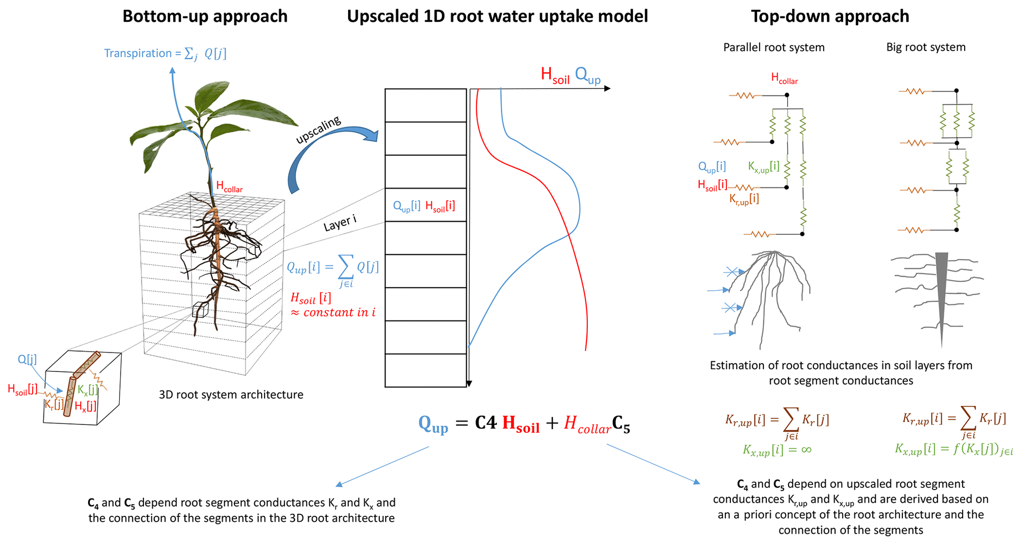
Figure 1Bottom-up approach versus top-down approaches for a parallel and a big root system model to derive and parameterize an upscaled one-dimensional root water uptake model.
The objective of this paper is to derive, with a bottom-up approach, an exact upscaled 1D model that describes root water uptake, considering the hydraulics of the 3D root architecture, and that could readily be implemented in land surface models. The model will be compared with parallel root and big root models that are currently used in 1D models. In order to interpret the models and their differences, we will cast in a first part the solutions of the models in a form that uses two hydraulic root system characteristics, namely the root system conductance and the root water uptake distribution for a uniform soil water potential or hydraulic head distribution. This was already done for a parallel root system by Couvreur et al. (2012), but an exact formulation of root water uptake in terms of these characteristics for a general root system model, including a 3D root model and its upscaled version and a big root model, is still missing. We will show that these characteristics are, for all models, sufficient to describe the total root water uptake as a function of soil and collar water potentials or hydraulic heads. We will further show that these root system characteristics fully define the parallel root model. Additional terms or factors in the equation for the exact root system can be used as diagnostics of the deviation between the parallel root system model and the exact 3D model or its upscaled version due to differences in root system topology. A second consequence of the parallel root model being fully defined by the two root hydraulic characteristics is that it can be parameterized straightforwardly in a bottom-up approach. In a second part, we will compare the upscaled exact model with the parallel and big root models that can be parameterized in two different ways, i.e., a top-down parameterization in which parameters are derived from the root segment distribution and root segment hydraulic parameters assuming a priori big root or parallel root topologies, versus a bottom-up parameterization of the parallel root model that uses exact hydraulic root system characteristics obtained from solving the flow equations in the 3D hydraulic root architecture (Fig. 1). For the parallel root system model, we can evaluate to what extent the simulated uptake is impacted by the simplified root system topology while using exact hydraulic root system characteristics. First, the models will be compared for a very simple hypothetical root system that represents a hybrid form of the two “asymptotic” root architectures (parallel root versus big root model). Second, the models will be compared for single roots with realistic distributions of root segment properties and for realistic root architectures of plants with a tap root or a fibrous root system.
The flow into and within a single root can be described using the porous pipe model (Landsberg and Fowkes, 1978) with the following equation:
where ℓ (L, where L refers to the physical quantity length) is the local axial coordinate of the root, kx (L3 T−1, where T refers to the physical quantity time) and kr (T−1) are the intrinsic axial and radial root segment conductances, r (L) is the root segment radius, and Hx (L) and Hsoil (L) are the hydraulic heads of the water in, respectively, the xylem and the soil in contact with the root, which include both the pressure potential and the elevation potential. Intrinsic conductances refer here to properties of the root segments that are independent of the axial discretization that we use to solve the equation. We can discretize this equation for a root system network that consists of Nroot root segments (edges) that are connected with each other in nodes (vertices). The entire network is connected to one outlet node that represents the root collar where the hydraulic head, Hcollar, or the flux boundary condition is defined. Since branches of a root architecture do not rejoin distally (further away from the collar), there is only one segment that connects a certain node with the proximal (closer to the collar) part of the root system or each node is the distal node of only one element (except for the collar node). Therefore, the network of Nroot root segments connects Nroot root nodes with each other and the root collar. The root nodes (but not the collar node) are connected by Nroot soil–root segments to Nroot soil nodes. The total number of segments (root segments connecting root nodes and soil–root segments connecting roots with soil nodes) is 2Nroot. The total number of nodes in this system, including the collar node, is 2Nroot+1. Each root node (except the collar node) can be linked uniquely to two segments, i.e., a root segment that connects the node to the proximal part of the root system and a soil–root segment that connects the node to the soil. The axial conductance Kx[i] (L2 T−1) of the proximal root segment and the radial conductance of the soil–root segment Kr[i] (L2 T−1) connected to the ith root node are defined as follows:
where l[i] (L) is the length, and r[i] (L) is the radius of the proximal root segment connected to the ith root node. The transpiration stream to the collar, T (L3 T−1), the xylem hydraulic heads, and the fluxes from the soil to the root nodes Q (L3 T−1) are obtained from solving the Laplacian matrix of the weighted directed graph of soil and root nodes, which is the discrete representation of the flow equation in the porous pipe root system as follows:
where IM is the () incidence matrix of the graph with 2Nroot+1 nodes and 2Nroot segments. The rows of the incidence matrix represent the nodes of the graph, and the columns are the segments. The first row represents the root collar, the next Nroot rows the root nodes, and the last Nroot rows the soil nodes. The first Nroot columns represent the root segments and the last Nroot columns soil–root elements. when node i is a distal node of element j, when i is proximal node of element j, and otherwise. Hx is the Nroot vector with xylem hydraulic heads in the root nodes, and Hsoil is the Nroot vector with the soil water hydraulic heads in the soil nodes. diag(K) is a diagonal conductivity matrix with the first Nroot diagonal elements representing the xylem conductivities and the last Nroot elements the radial conductances. 0 is an Nroot vector with zeros, and Q is the Nroot vector with fluxes from the soil nodes to the root nodes. The derivation of Eq. (4) is demonstrated in the Appendix. The first equation represents the total transpiration stream out of the network as a function of the hydraulic heads in the root collar and the root nodes connected to the collar and the axial conductances of the root segments connected to the root collar. The next Nroot equations close the water balances in root nodes, and from solving these, the xylem hydraulic heads in the root nodes are obtained. The last Nroot equations yield the fluxes Q from the soil nodes to the root nodes.
Plugging the obtained xylem hydraulic heads in the last Nroot equations, the fluxes towards each root node are obtained from Eq. (4) (see the Appendix) as follows:
where C4 (L2 T−1) is an Nroot×Nroot symmetric matrix and C5 (L2 T−1) an Nroot×1 column. The relations between C4, C5, the root segment conductivities (stored in diag(K)), and the segment connections (defined in the incidence matrix IM) are given in Table 1. This equation can be written in another form that uses macroscopic characteristics of the root system, i.e., the root system conductance, Krs (L2 T−1), and the standard uptake fraction vector SUF (Nroot×1) of the root nodes that were introduced by Couvreur et al. (2012). Krs relates the total root water uptake to the difference between an average or effective soil water hydraulic head, Heff (L) and Hcollar as follows:
SUF[i] represents the fraction of the total uptake by the ith root node for a uniform Hsoil. In the Appendix, we derive that Heff corresponds with the SUF-weighted average of Hsoil as follows:
Equation (7) implies that the effective soil water hydraulic head depends more strongly on soil water hydraulic heads where the root system takes up more water when the soil water hydraulic head is uniform. Equations (6) and (7) imply that Krs and SUF are sufficient root system properties for calculating the total root water uptake. Using these macroscopic root system characteristics, Eq. (5) can be rewritten as follows:
where Heff is a (Nroot×1) vector filled with Heff. The derivation of Eq. (8) is given in the Appendix, and we summarize the main properties of the equation here. The first term on the right-hand side of Eq. (8) represents the uptake from the soil profile when the soil water hydraulic head is uniform and equal to Heff. The definition of Heff as the SUF-weighted average of Hsoil makes that the sum of the fluxes of the second term of the right-hand side of Eq. (8) becomes zero (see Eq. A33). The second term on the right-hand side represents the increase (decrease) in the amount of water that is taken up by a root node that is connected to soil node where Hsoil is higher (lower) than Heff. This second term represents the compensatory uptake, and we name the C4 matrix the compensatory matrix. Of note is that the second term only depends on the hydraulic root architecture (defining C4 and SUF) and on the soil water hydraulic head distribution. It neither depends on the water potential at the root collar nor on the transpiration rate. As a consequence, root water uptake compensation changes over time only due to changes in the soil water hydraulic heads but not due to, e.g., diurnal changes in transpiration rate. In Table 1, relations between Krs, SUF, C4, Heff, and the root hydraulic architecture are given.
Table 1Equations to calculate the root system hydraulic conductance, Krs, the standard uptake fraction, SUF, and the compensatory uptake matrix, C4, from the hydraulic root architecture.

Krs and SUF can be calculated directly from the compensatory matrix C4. In the following, we will present a reformulated form of Eq. (8) that resembles the equation that is obtained for a parallel root system. For the derivation, we refer to the Appendix, and we focus here on the results.
As is derived in the Appendix, the matrix C4 in Eq. (8) can be “factorized” in a product of two diagonal matrices, i.e., one with a diagonal that is equal to the SUF vector and one with a diagonal that represents a “compensatory conductivity vector” Kcomp. There is also one matrix C7, which is close to the identity matrix I, so that Eq. (8) can be rewritten as follows:
The diagonal elements of C7 are 1, and for each row of C7, the sum of the off-diagonal elements is equal to zero. To explain the meaning of Kcomp and how it is related to Krs in the parallel root system model, we consider a soil water hydraulic head distribution that is uniform except for one node i, where the hydraulic head is ΔH higher than in all other nodes ( for all j≠i). We, furthermore, put Hcollar equal to Heff so that there is no net uptake but only redistribution of water through the root system. Then the flow from node i to all other nodes in the root system, ΔQ[i], is as follows:
where kcomp[i] (L3 T−1) represents the conductivity of the root system to transfer water from all other root elements to the root node i. From the definition of Heff, it follows that:
Using this Hsoil−Heff in Eq. (17), from the soil hydraulic heads Hsoil[j] being all the same for the soil nodes j and different from i and from the off-diagonal elements of a row in C7 summing up to zero, it follows that ΔQ[i] is:
By comparing Eqs. (18) and (20), we find that SUF[i](1−SUF[i]) Kcomp[i]=kcomp[i].
For a root system in which all root nodes are connected in parallel to the root collar, kcomp[i] is equal to the equivalent conductance of a serial connection of a conductance from root node i to the collar, which is SUF[i]Krs, with a conductance from the collar to all other nodes, (1−SUF[i])Krs, and it follows that:
This implies that, for a parallel root system, Kcomp=Krs. It can further be shown that C7 is the identity matrix for a parallel root system (see Appendix), so that Eq. (8) can be written as follows:
The parallel root system is fully defined by the SUF and Krs, and the compensatory uptake is defined when the uptake distribution from a soil profile with a uniform soil water hydraulic head is known. This implies that any root system can be represented by a parallel root system with the same SUF and Krs that simulates the same total root water uptake for any distribution of soil water hydraulic heads. However, comparing Eq. (22) with Eq. (17) shows that the compensatory uptake between the root system and its parallel root analogue differs and that diag(Kcomp) and C7 can be used as diagnostics for the difference in compensatory uptake. For the general root system, we find that Kcomp[i] is larger than Krs. This means that for a certain ΔH between soil node i and all other nodes, there is more redistribution in the general root system than in the parallel root system. In the general root system, the flow from one soil–root interface to another soil–root interface does not always have to pass through the collar but can take a shorter way. A negative value of C7[i,j] means that, for a given hydraulic head difference between two nodes i and j, there is more redistribution between node i and j than the average redistribution for this head difference between node i and another node than node j of the network. This means that node i is stronger than the average connected to node j.
From the matrix equations, it follows that the upscaling of the relations between the uptake rates Q and soil water hydraulic heads Hsoil is trivial for cases when the soil water hydraulic heads are uniform in certain regions of the soil. When we assume that the soil water hydraulic heads do not change in the horizontal direction, then we can simply group and sum up all SUF values for the soil root nodes that are in the same soil horizontal soil layer and derive an upscaled SUF vector that describes the relative uptake from each soil layer when the soil water hydraulic heads are uniformly distributed (Couvreur et al., 2014a; Fig. 2). The upscaled matrix C4 that is multiplied by a vector of soil water hydraulic heads in the different soil layers is simply obtained by the following:
The dimensions of the upscaled matrices are reduced so that the number of equations that need to be solved is reduced to the number of layers in which the soil water hydraulic heads are uniform. This implies a massive reduction in the computational cost compared with the cost of solving equations for a large number of root segments that make up a 3D root architecture. Under the assumption that the soil water hydraulic heads are constant within a layer, the obtained equations are exact, independent of the soil water hydraulic heads, and need to be derived from the large set of equations for a given 3D root architecture only once. They can be used afterwards to calculate uptake from the layers for other collar and soil hydraulic heads. Based on the upscaled C4 and SUF, the upscaled C7 and Kcomp can be derived. It must be noted that C7 and Kcomp cannot be scaled up directly by summing up elements in the C7 matrix and Kcomp vector. When the 3D root architecture is a parallel root architecture, then the upscaled model has the same form as Eq. (22) in which the upscaled SUF is used. This upscaled model represents an upscaled parallel root system with each root connecting one soil layer with the to the root collar. It should be noted that we did not derive an “upscaled” root system topology for the exact model. In the following, we will always refer to the upscaled parallel root model. The upscaling was performed here assuming uniform soil water hydraulic heads in the horizontal direction. It can be applied for any region where soil water hydraulic heads are assumed to be uniform. The upscaled parallel root model then represents a root system with parallel roots that each connect one region with the root collar.
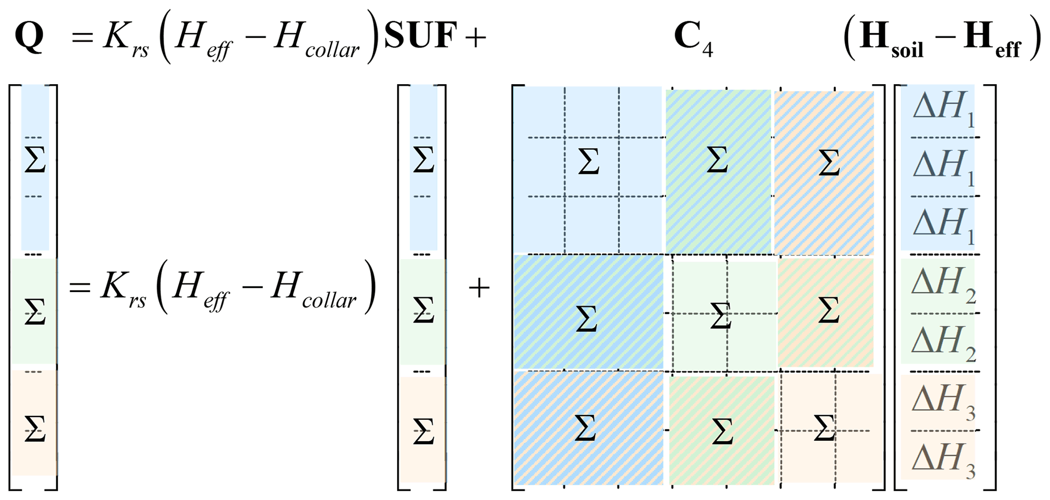
Figure 2Upscaling of the SUF and C4 matrix by simply taking the sum of elements that correspond with nodes where the soil water hydraulic heads are the same. Nodes with the same water hydraulic heads are grouped in layers and are marked with the same color. The elements of the marked blocks of the Q and SUF vectors and in the C4 matrix are summed up.
In order to demonstrate the model, its upscaling, and comparison with big root and parallel root approximations, we considered in a first step an abstract “hybrid” parallel–big root system, which is a mixture of the parallel and big root systems. It consists of three parallel branches of different length that each take up water along their length and not only at the root tip, as supposed in the parallel root system. Since the water fluxes in each of the three branches are different because of their different lengths, the water hydraulic heads in the xylem at a given depth differ between the three roots even when the soil water hydraulic heads do not vary at a given depth. Therefore, this hybrid root system represents an intermediate model that neither matches with the parallel root nor the big root model perfectly. This model should demonstrate the upscaling and the difference between the approximate models. We used a dummy parameterization of the root hydraulic properties and of the vertical distribution of the soil water hydraulic heads (i.e., the parameters were chosen to represent certain differences but the actual values of the parameters and their units were not of interest). We considered a case in which all the root segments had the same radial conductance and a case in which the radial conductance at the root tips were a factor of 10 larger.
In a second step, we considered a single root with either constant or changing root hydraulic parameters along the root axis.
In a third step, we considered root systems that correspond, in terms of complexity and parameterization, to more realistic root systems and represent three different crops of grass, maize, and sunflower.
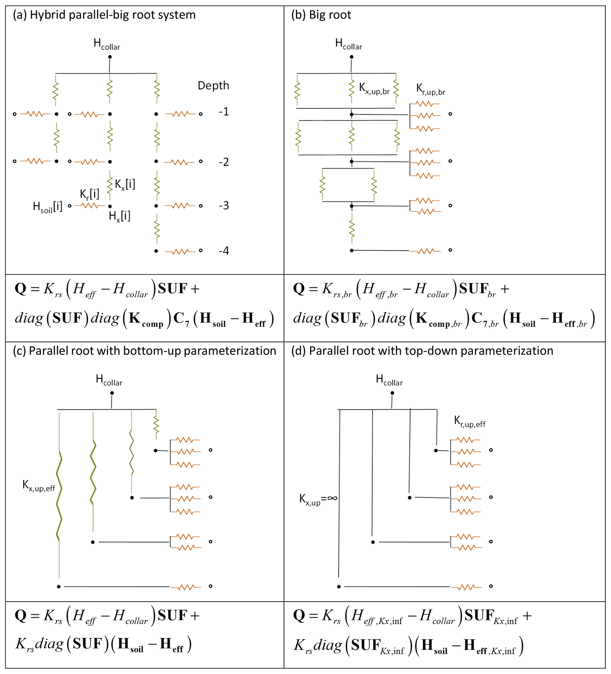
Figure 3Resistance nets representing the hybrid parallel–big root system consisting of three primary root branches of different lengths (a). There are also approximations by the big root model (b), the parallel root model using a bottom-up parameterization (c), and the parallel root model with a top-down parameterization (d). The closed circles represent root nodes and the open circles soil nodes; the brown and green resistors represent radial and axial root segment conductances, respectively. The approximate models describe upscaled root water uptake from four depths. The SUFbr, Krs,br, Kcomp,br, and C7,br of the big root model are calculated from the segment axial and radial conductances that are arranged following the big root topology in parallel within a soil layer from which upscaled big root segment conductances Kr,up,br and Kx,up,br are calculated (top-down parameterization). The SUF and Krs of the parallel root model with bottom-up parameterization (c) are matched to those of the upscaled hybrid model by adapting the axial conductance Kx,up,eff of the segment that connects the xylem node at a certain depth to the collar node. The SUF of the parallel root model with top-down parameterization, assuming infinite Kx,up (d), is derived from the distribution of radial root segment conductances with depth, which are scaled to Kr,up,eff so that Krs matches that of the hybrid root system. The equations below the resistance nets represent the equations that calculate the upscaled water uptake Q in a horizontal layer.
4.1 Simple hybrid root system
Figure 3a shows the hybrid parallel–big root system that consists of three primary root branches of different length which take up water from up to four different depths. This root system was scaled up to a model that describes uptake from the four depths, assuming that the soil water hydraulic head is uniform at a given depth (the exact model). The upscaled SUF, which represents the uptake by all root segments at a certain depth, was equal to the sum of the SUFs of the individual root segments at that depth. The upscaled hybrid parallel–big root system model was approximated by parallel and big root system models. The big root approximation assumes that the root segments are organized and connected, following the a priori defined big root architecture, so that the upscaled axial Kx,up,br and radial Kr,up,br conductance in a certain layer is the sum of the axial and radial conductances of the individual root segments in that layer (Fig. 3b). Since we assume a priori a certain topology of the root segments and parameterize the model directly, based on the number of root segments in a soil layer and their properties (radial and axial conductances), we called this a top-down parameterization. For the parallel root approximation, we considered a root system with the same SUF and Krs as the upscaled hybrid model (Fig. 3c). For a given distribution of radial conductances, Krs and SUF can be defined by adapting an upscaled effective Kx,up,eff of virtual root branches that connect a certain depth with the root collar. This parameterization, which is based on calculations for the 3D hydraulic root architecture, corresponds with a bottom-up parameterization. For the upscaled parallel root model, the number of parameters that needs to be defined is equal to the number of soil layers, ndepths, i.e., ndepths Kx,up,eff values or Krs and ndepths−1 SUF values (sum of SUF=1). In contrast, the big root model requires two ndepths parameters. Unlike for the parallel root system, there is no simple relation between Krs and SUF, on the one hand, and the compensatory uptake term, on the other, for the big root model. Therefore, the structure of the big root model does not lend itself to calculating its parameters directly from characteristics of the 3D hydraulic root architecture in a bottom-up approach. The third model that we considered is a parallel root model with an infinitely large axial conductance (Kx,up=∞) in which the SUF is derived in a top-down approach directly from the distribution of the upscaled radial conductances, Kr,up,eff, with depth. The Krs of this root system was adjusted to the Krs of the hybrid root system, which comes down to a scaling of the radial conductance of all root nodes with the same factor.
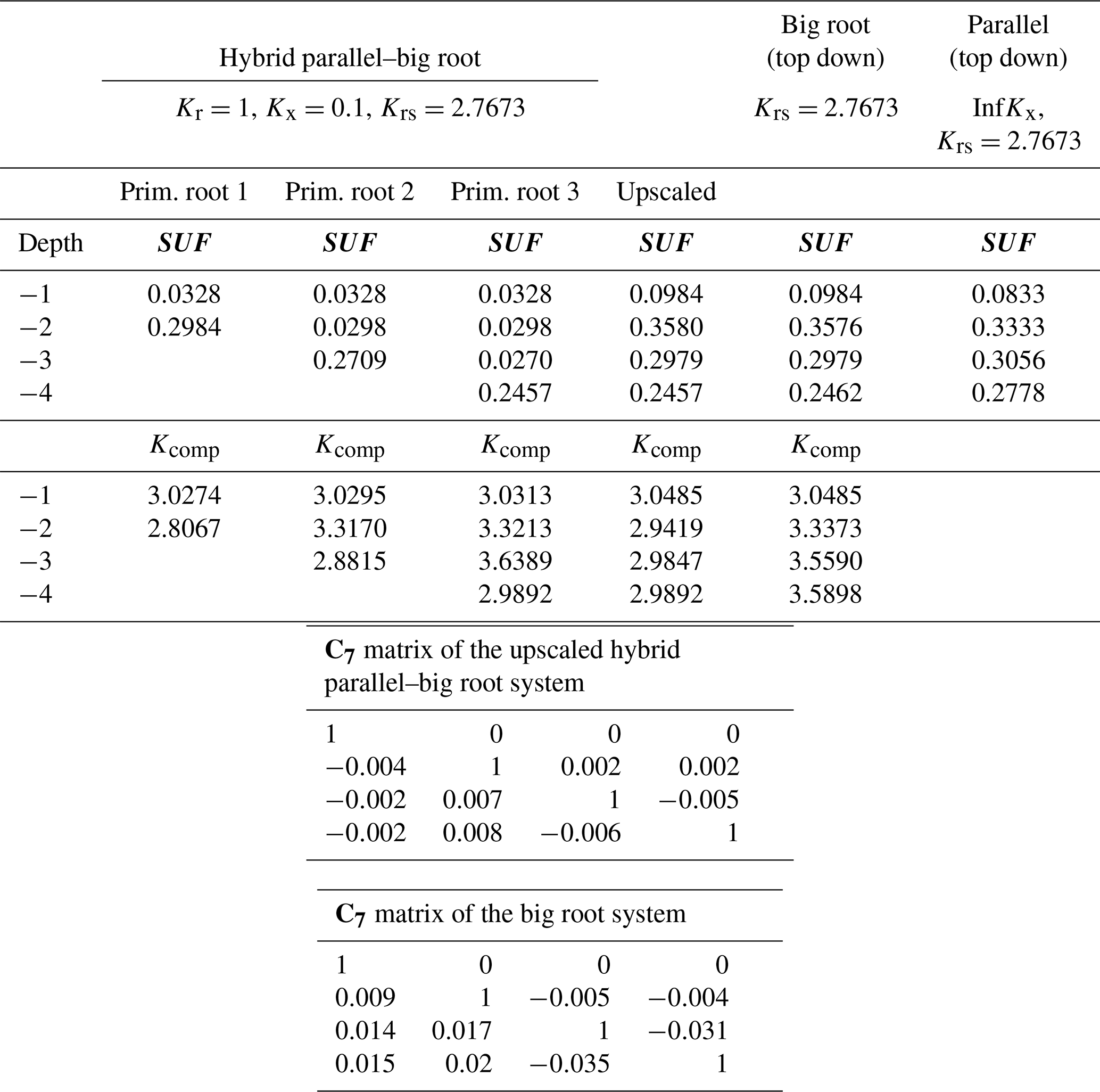
We considered two parameterizations of the root hydraulic conductances. In the first case, the conductances of all root segments are uniform, i.e., Kx=10 and Kr=1. In the second case, the radial root hydraulic conductance is larger at the root tips (Kr=1) than in the other parts along the primary roots (Kr=0.1). To evaluate the effect of a non-uniform hydraulic head in the soil, the soil water hydraulic heads varied from top to bottom as −0.5, 0, 0.5, and 1 and were assumed to be the same for root nodes at the same depth. The hydraulic head at the root collar was set to −1. The Krs, SUF, and Kcomp, their upscaled values for the hybrid root system, and the three approximations are given in Tables 2 and 3 for the root system with homogeneous root segment conductances and for the root system with higher radial conductances at the root tips, respectively. The root water uptake profiles that are simulated by the different models for the two parameterizations of the root segment conductivities are given in Figs. 4 and 5.
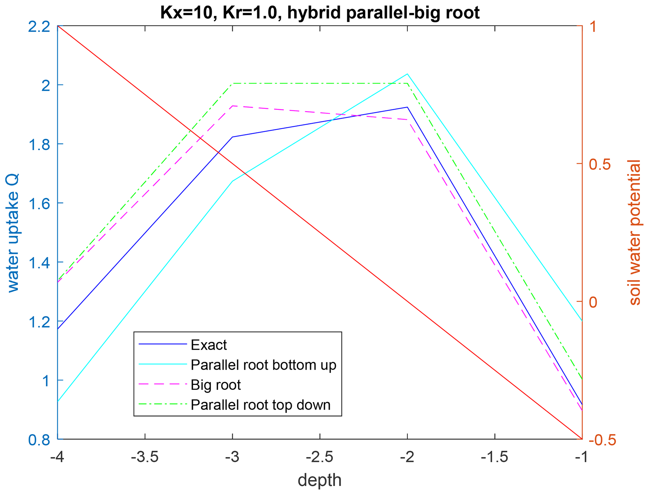
Figure 4Upscaled water uptake profile (left axis) and soil water potential distribution (right axis; red line) for the hybrid parallel–big root system with constant radial conductances along the primary root branches, with the parallel root model with bottom-up parameterization (SUF and Krs derived from the exact model), the big root model, and the parallel root model with top-down parameterization.
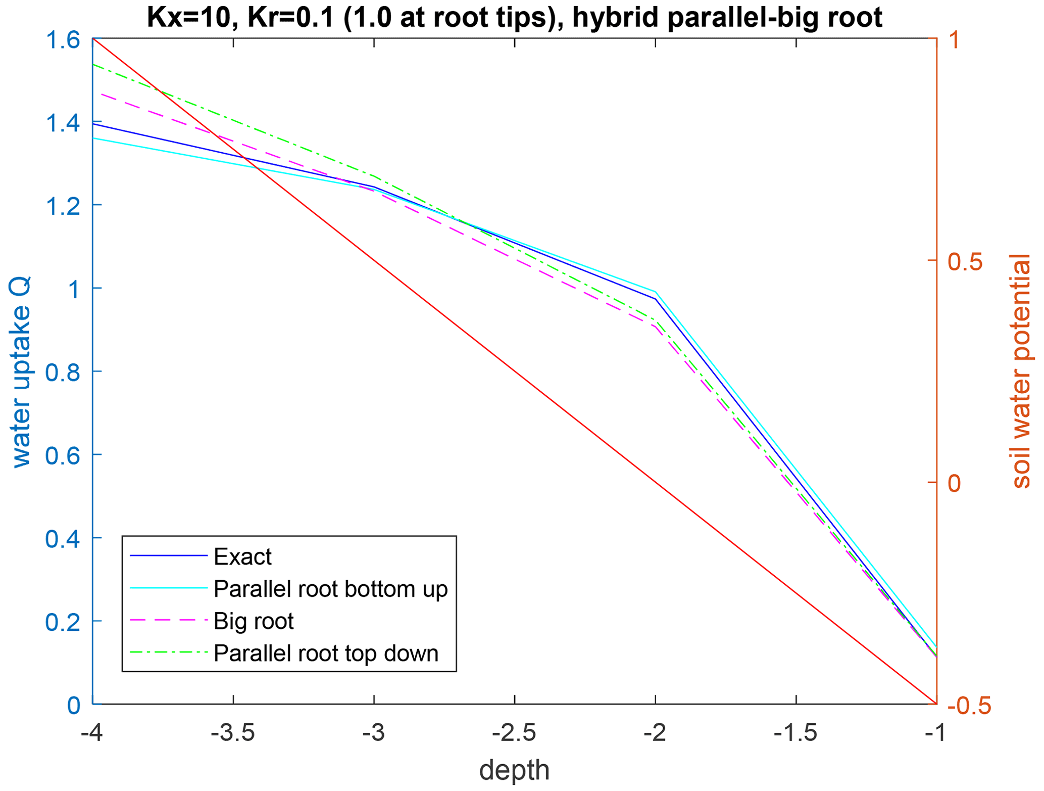
Figure 5Upscaled water uptake profiles (left axis) and soil water potential distribution (right axis; red line) for the hybrid parallel–big root system with radial conductances along the primary root branches that vary along the branches (radial conductance is 1 at root tips and 0.1 at other nodes), with the parallel root model with bottom-up parameterization (SUF and Krs derived from exact model), the big root model, and the parallel root model with top-down parameterization.
Table 2Krs, SUF, Kcomp, and upscaled values and C7 matrices for the hybrid parallel–big root system with constant Kr along the roots, the big root system, and the parallel root system (with infinite Kx) using top-down parameterization.
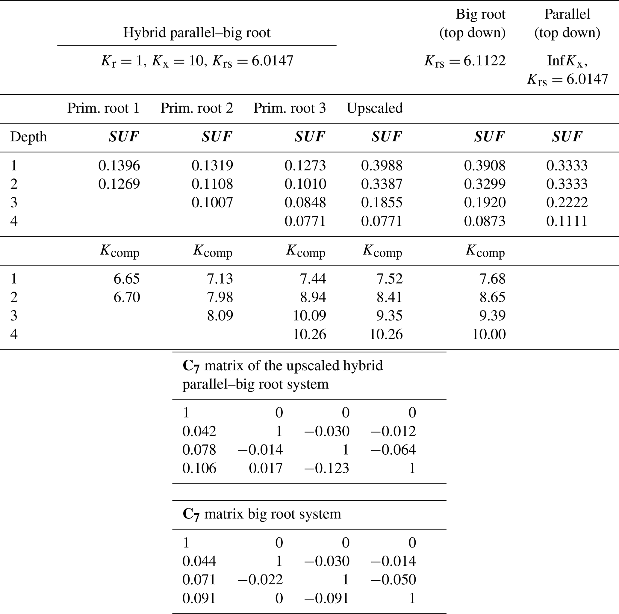
Table 3Krs, SUF, Kcomp, and upscaled values and C7 matrices for the hybrid parallel–big root system with variable root radial root segment conductances along the roots (Kr=0.1 along roots, except at root tip Kr=1) for the big root system and for the parallel root system (with infinite Kx) using top-down parameterization.
The parallel root system with a top-down parameterization and using the distribution of root segment radial conductances with depth to estimate SUF overestimates the SUF deeper in the soil profile and underestimates it at shallower depths. The resistance to axial flow reduces the SUF of distal root segments compared to the SUF of more proximal root segments. The big root model can better account for the impact of the axial resistance on the SUF. However, the assumption of equal xylem hydraulic head in all root segments at a certain depth leads to an underestimation of the SUF of the proximal root segments (Table 2). This underestimation was not important when the radial conductance was larger near the root tips (Table 3).
For a non-uniform distribution of the soil water hydraulic head, which increased with depth, the uptake increased at greater depths and decreased at shallower depths, as compared to the uptake under the uniform soil water hydraulic head (Figs. 4 and 5). All models reproduced this compensation of root water uptake. The parallel root model with bottom-up parameterization, which used the exact root system SUF and Krs, underestimates the root water uptake compensation, whereas the big root model overestimates it. The parallel root model uses Krs to calculate the compensatory uptake, and Krs was smaller than Kcomp (Tables 2 and 3). The big root model overestimates the compensation since it assumes that all root segments in a certain layer are directly connected to all the root segments in the overlying or underlying layers and that the xylem hydraulic heads are the same in all root segments at a certain depth. This implies that the redistribution of water between the soil layers via the root system can occur directly without flow having to pass the collar first before it returns to another layer. The Kcomp that is derived for the big root model is only slightly higher, except for the deepest root node, than the Kcomp of the exact model. The larger uptake from the deeper layer simulated by the big root model is, therefore, linked to the larger SUF in the deeper soil layers. This is also the case for the parallel root model with bottom-up parameterization for which the higher SUF at greater depths in combination with higher soil water hydraulic heads at greater depths led to a larger simulated water uptake.
Also of interest is that the upscaled Kcomp values are not equal to the average of the Kcomp values of the root nodes in a soil layer. For the top layer, the upscaled Kcomp is even larger than the largest Kcomp value of the three primary root branches. Smaller radial conductance away from the root tips led to a root system that behaves more like a parallel root system (Fig. 5). This is reflected in the Kcomp values that are closer to Krs and the C7 matrix that is closer to the identity matrix than the C7 matrix of the hybrid parallel–big root system with uniform root segment hydraulic properties (Table 3). The higher radial root segment conductances near the root tips allow the water transfer between two soil layers through root tips in these soil layers, which passes via the root collar, to be more efficient than water transfer between a root tip segment and a root segment with lower radial conductance that is directly connected to it. In the big root model, the root tip segment with higher radial conductance in one layer is assumed to be directly linked to the root tip segment in another layer so that the water flow between these layers occurs more efficiently than via the root collar. This is reflected in the higher Kcomp and the larger deviation in the C7 matrix from the identity matrix for the big root model than for the hybrid parallel–big root model, which leads to an overestimation of the root water uptake compensation by the big root model.
4.2 Single root branches
We considered two single root branches, one with homogeneous (intrinsic) root segment conductances (kx=0.171 cm3 d−1, d−1) and one with conductances that changed along the root axis due to maturation of the root tissue (Fig. 6). This generally leads to an increase in axial conductance and a decrease in radial conductance with age or distance from the root tip (Doussan et al., 1998, 2006; Zarebanadkouki et al., 2016; Couvreur et al., 2018; Meunier et al., 2018b). The “reference” exact model was a 50 cm long root discretized in 0.5 cm long root segments.
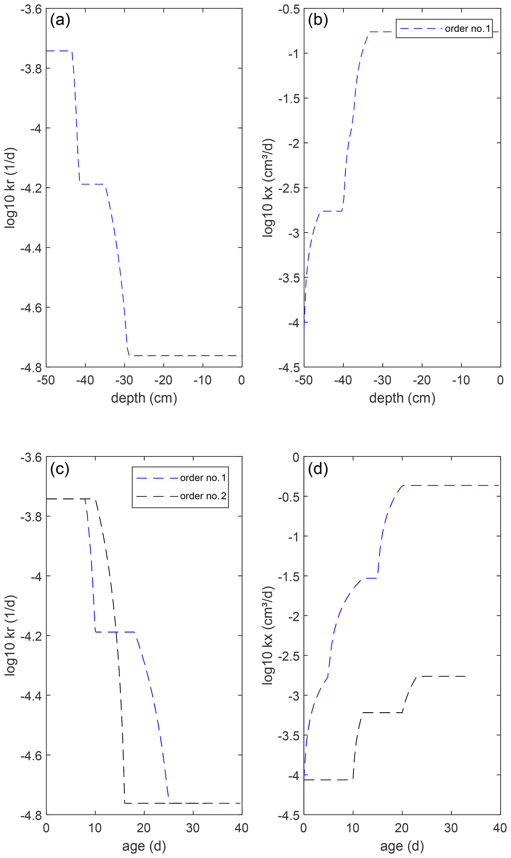
Figure 6Radial (a, c), kr, and axial (b, d), kx, intrinsic root conductances for the single root (a, b) and root system architectures (c, d). For the single root, conductances are plotted versus depth and for the root system architectures versus root segment age.
The collar water hydraulic head was assumed to be −4000 cm, and the soil water hydraulic head varied linearly between −3000 cm at the soil surface and 0 cm at the lowest depth of the root system. The upscaled model considered 2 cm long segments.
As expected, the big root system matches nearly perfectly with the exact model (Fig. 7). The deviations are due to the upscaling and the variations in soil water and xylem hydraulic heads along a root segment that is represented by a single node (Bouda, 2019). Nevertheless, the close agreement indicates that the 0.5 cm discretization of the root approximates the exact solution of the flow equation in the single root well. Details on the convergence of this discretization and on exact solutions for arbitrary root segment sizes (given that the soil water potentials do not vary along the root segments) are given by Meunier et al. (2017b, c). For large root segment sizes or small Kx, when the discrete approximation becomes inaccurate, exact solutions can be implemented in a complex root architecture (see Bouda, 2019), but this should lead to a different coefficient matrix C4 and C5 vector. The parallel root model with a top-down parameterization that derives the SUF based on the radial root segment conductances assuming an infinite Kx overestimates the SUF in the distal part of the root since the impact of the axial resistance to flow is not considered. For a larger soil water hydraulic head near the distal end of the root, the overestimation of the SUF in this region results in an overestimation of the root water uptake from the deeper soil and an overestimation of the apparent root water uptake compensation. The opposite is the case for the parallel root system with a bottom-up parameterization, which uses the exact SUF. This model underestimates the uptake near the distal end of the root due to an underestimation of Kcomp by the parallel root model. However, for a root with non-uniform root segment conductances, uptake simulated with this parallel root system represents nearly perfectly the exact uptake and even slightly better than the big root system. Even for a single root, which can be considered to be a “perfect” big root system, the parallel root model may perform quite well when it uses the exact SUF. This is even better when root segment conductivities vary along the root. The Kcomp profiles and C7 matrices, which are shown for the two root systems in Fig. 8, may be used as diagnostics of the approximation of the root water uptake by the parallel root model. Rather than the absolute values of the ratios of and of the entries in the C7 matrix, the distributions of these values along the root profile seem to indicate whether a parallel root model can describe the uptake profile. For the root with uniform root segment conductances, larger values of and off-diagonal entries in C7 that deviated from zero were distributed more over the entire root length, whereas for the root with non-uniform root segment conductivities, these larger values and deviations were concentrated near the root tips.
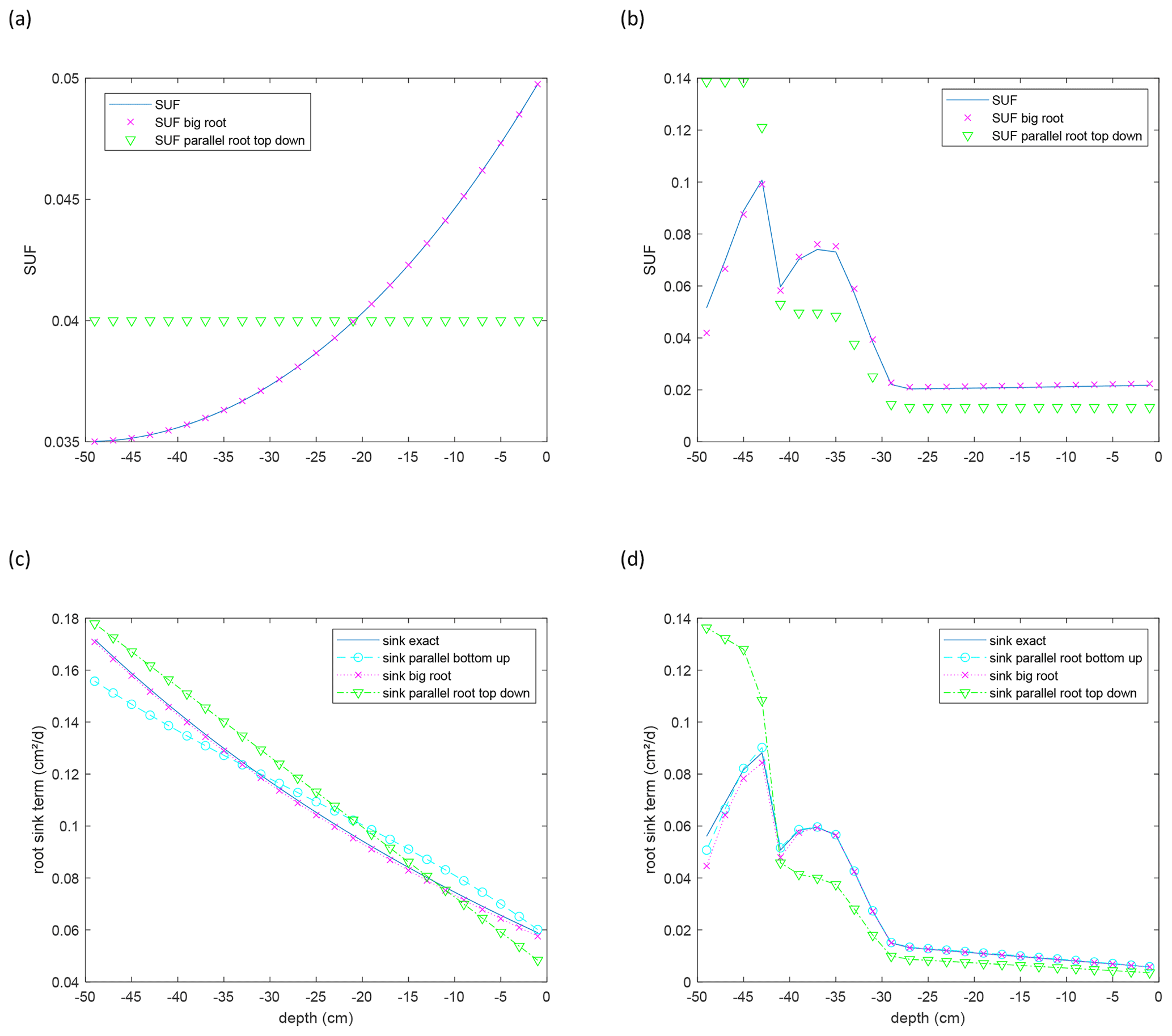
Figure 7Standard uptake for homogeneous soil water potential (SUF) (a, b) and root sink term for a linear increase in water potential with depth (c, d) of a single root branch with uniform (a, c) and age-dependent (b, d) root segment conductances. Approximations are calculated for the parallel root with a bottom-up parameterization using the exact SUF and Krs, the big root model, and parallel root model with a top-down parameterization, with SUF estimated from the radial root segment conductivities. Sink terms are divided by the thickness of the soil layer, 2 cm, over which the root segment sink terms are summed.

Figure 8C7 matrices and profiles of the ratio of of the exact single root model with uniform (a) and non-uniform (b) root segment hydraulic conductances along the root. The labels on the axes of the C7 matrices represent the root segment numbers, which increase from the proximal to the distal end of the root, i.e., from top to bottom. For visualization, the diagonal elements of the C7 matrix were set to 0.
4.3 Realistic root systems
We generated root systems of three different plants, i.e., maize, sunflower, and grass, using the CRootBox shiny app (https://plantmodelling.shinyapps.io/shinyRootBox/, last access: 27 August 2021; Schnepf et al., 2018). The grass root system with several primary roots and few laterals may represent a parallel root system. The maize root system, with several primary roots that each take up water along their axis by lateral roots, may represent a hybrid parallel–big root system, whereas the sunflower root system with a single main root and several lateral roots might rather represent a big root system (Fig. 9). The intrinsic radial and axial root segment conductances depended on the root order and varied with age (Fig. 6). We assumed that this relation between root age and segment conductance did not vary between the crops. It should be noted that the root architectures and intrinsic root segment conductances were chosen to illustrate the difference between the different root water uptake modeling approaches for more realistic root systems. However, the derived root system characteristics should not be interpreted as the characteristics of a certain crop. As for single root branch simulations, the collar water potential was −4000 cm, the soil water potential at the soil surface −3000 and 0 cm at the maximal rooting depth of the root system. The SUF and root water uptake distributions were scaled up to and derived for 2 cm thick horizontal soil layers yielding 1D vertical profiles.

Figure 9Root systems generated with the CRootBox shiny app. (a) Maize. (b) Sunflower. (c) Grass. Colors refer to the root order.
For the parameterization of the big root model, we calculated the axial conductance of the big root for each soil layer i, Kx,up,br[i], from the length, orientation, and intrinsic axial conductances of all the root segments in that layer as follows. First we calculated an “effective” intrinsic axial conductance for flow in the vertical direction in the ith soil layer, kx,eff,[i], as follows:
where α[j] is the angle of the segment with the vertical, and j is the indices of root segments in layer i. To obtain Kx,up,br[i], we multiplied the effective intrinsic axial conductance by the number of roots that cross the layer and divided it by the layer thickness. The number of roots that cross the layer i is calculated from the sum of the vertical increments of the root segments divided by the layer thickness so that we obtained the following:
The radial conductance of the big root system in layer i, Kr,up,br[i], was calculated by simply adding up the radial conductances of the root segments.
For the parallel root system with bottom-up parameterization, we used the SUF and Krs values of the exact upscaled model. For the parallel root model with the top-down parameterization, assuming an infinite Kx, the SUF was directly calculated from the distribution of the radial root segment conductances that were upscaled as in the big root model as follows:
To account for the effect of resistance to axial flow, the exact Krs is used in the top-down parameterized parallel root model. It should be noted that Eqs. (24), (25), and (26) use information about root segments, such as their orientation, age, root-type-dependent conductance, and surface, which is mostly not used or available to parameterize macroscopic hydraulic root water uptake models. Mostly, the root segment conductances and root radii are assumed to be constant so that root length density is used to estimate the hydraulic properties. Since we focus in this paper on the differences between different model structures, we used the more detailed information to avoid differences due to differences in information that was used for parameterization.
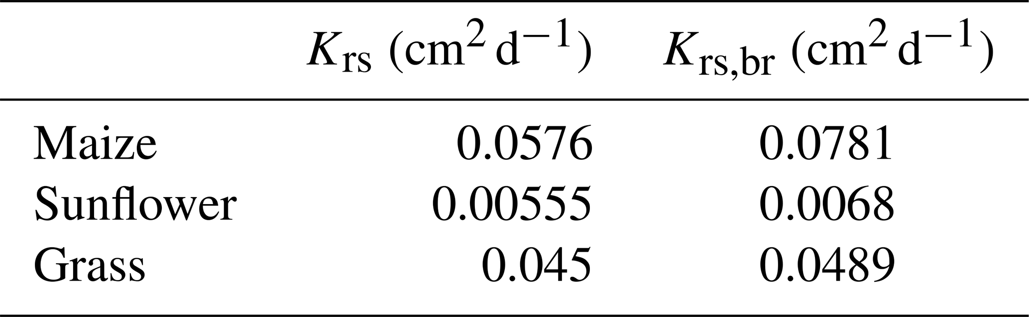
The root system conductances that are estimated from the root segment conductances, considering the 3D hydraulic root architectures, Krs, or using a big root representation, Krs,br, are given in Table 4. The root system conductances for sunflower are considerably smaller than those of maize and grass. This is attributed to sunflower having only one single tap (primary) root with a high intrinsic axial conductance (Fig. 6) versus maize and grass having many primary roots. Krs,br is larger than the exact Krs. The top-down parameterization of the big root model (Eqs. 24 and 25) in combination with the assumption that the root architecture can be represented by a single big root leads to an overestimation of the root system conductance. This was also observed for the simple hybrid parallel–big root model (Table 2).
Table 4Root system conductances, Krs, and root system conductances of the big root model, Krs,br, estimated from root segment conductances.
For the grass root system, which consists of several short primary roots with high axial conductance, SUF is almost not sensitive to the assumed root architecture (Fig. 10e). For the maize and sunflower root systems, the parallel root system using a top-down parameterization and assuming no axial resistance to flow underestimated the SUF at shallower depths and overestimated it at intermediate (maize) and deeper (sunflower and maize) depths (Fig. 10a and c). Not considering axial resistance to flow leads to an overestimation of the uptake capacity of the distal ends of roots, especially when the axial conductivity decreases and the radial conductance increases towards the root tip (see also Fig. 7b). Depths where the SUF is strongly overestimated correspond with depths with high densities of younger lateral roots. The SUF of the big root model corresponded better with the exact SUF. But, in the big root model, the axial resistance to flow from the distal ends of the deep primary roots to the collar is apparently overestimated and the SUF in the deeper soil layer underestimated. In the big root model, the xylem water potentials in the secondary and primary roots in a certain layer are assumed to be equal, since it is assumed that all root segments in a layer act in parallel. However, because of the lower axial conductance of secondary roots (see Fig. 6) which are connected in series to primary roots, the xylem water heads can be considerably higher in the secondary than in the primary roots in a certain layer. Assuming similar xylem water heads in secondary and primary roots in a certain soil layer reduces the xylem heads in the secondary roots and generates too much uptake by the secondary roots in that layer. An overestimation of uptake in a more “downstream” or shallower soil layer will lead to an underestimation in the more “upstream” or deeper layers. These effects may explain the underestimation of the SUF below approximately 50 cm depth in the maize and sunflower root systems that is compensated by an overestimation in shallower depths.
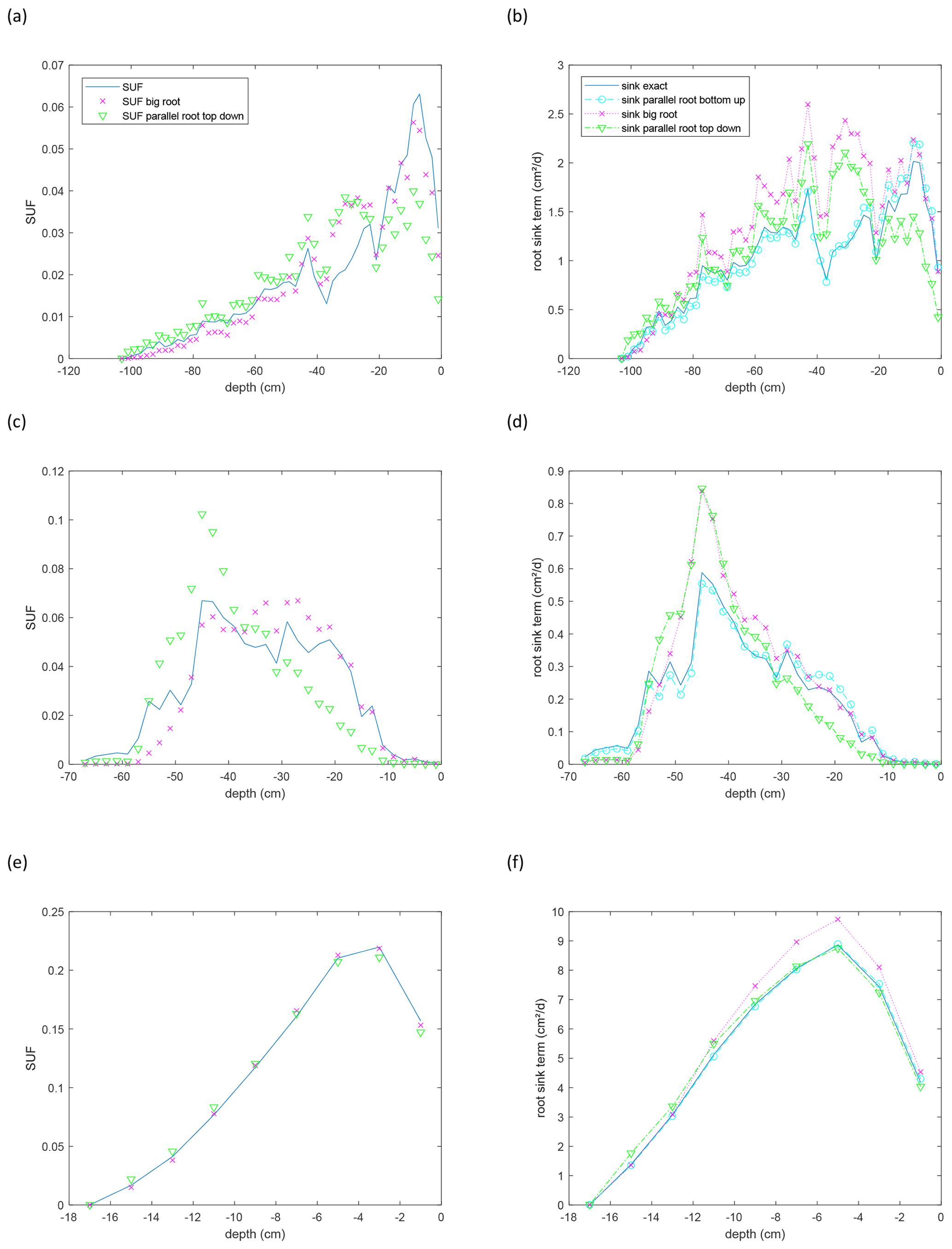
Figure 10Depth profiles of scaled up standardized uptake fractions (SUFs) (a, c, e) and sink term distribution normalized by the considered soil layer thickness (2 cm) for a non-uniform soil water potential distribution (−3000 cm at the soil surface and 0 cm at the maximal root depth) (b, d, f) for the maize (a, b), sunflower (c, d), and grass (e, f) root systems shown in Fig. 9. Approximations are calculated for the parallel root with a bottom-up parameterization using the exact SUF and Krs, the big root model, and the parallel root model with a top-down parameterization, with SUF estimated from the radial root segment conductivities. Sink terms are divided by the thickness of the soil layer, 2 cm, over which the root segment sink terms are summed.
The non-uniform soil water hydraulic heads resulted in an increased uptake deeper in the soil profile (compare the shape of the SUF and sink term profiles in Fig. 10). For the grass root system, the sink distributions for the different models are very similar. The higher uptake predicted by the big root model is due to the higher Krs,br than the true Krs. For the other root system models, the differences between the sink term distributions of the exact model, the big root model, and the parallel root model with top-down parameterization, assuming infinite axial conductance, are caused by differences in Krs, SUF, and compensatory uptake resulting from approximations of Kcomp and the C7 matrix (Fig. 11). The parallel root model with bottom-up parameterization that uses the exact Krs and SUF profile but approximates Kcomp by Krs and C7 by the identity matrix, predicts almost the same sink term distribution profile as the exact model. This bottom-up parallel root model slightly underestimates the compensatory root water uptake, i.e., too much uptake near the soil surface and too little deeper in the soil profile. The exact trace and C7 matrix of the root systems (Fig. 11) suggest the largest deviations between the sink term distributions of the exact model and the bottom-up parallel root model for the sunflower root system, which corresponds with the results shown in Fig. 10. The impact of approximations of Kcomp and the C7 matrix on the sink term distribution is apparently of second-order importance compared to the impact of the estimated Krs (big root model) and SUF (big root model and top-down parallel root model with infinite axial conductance).
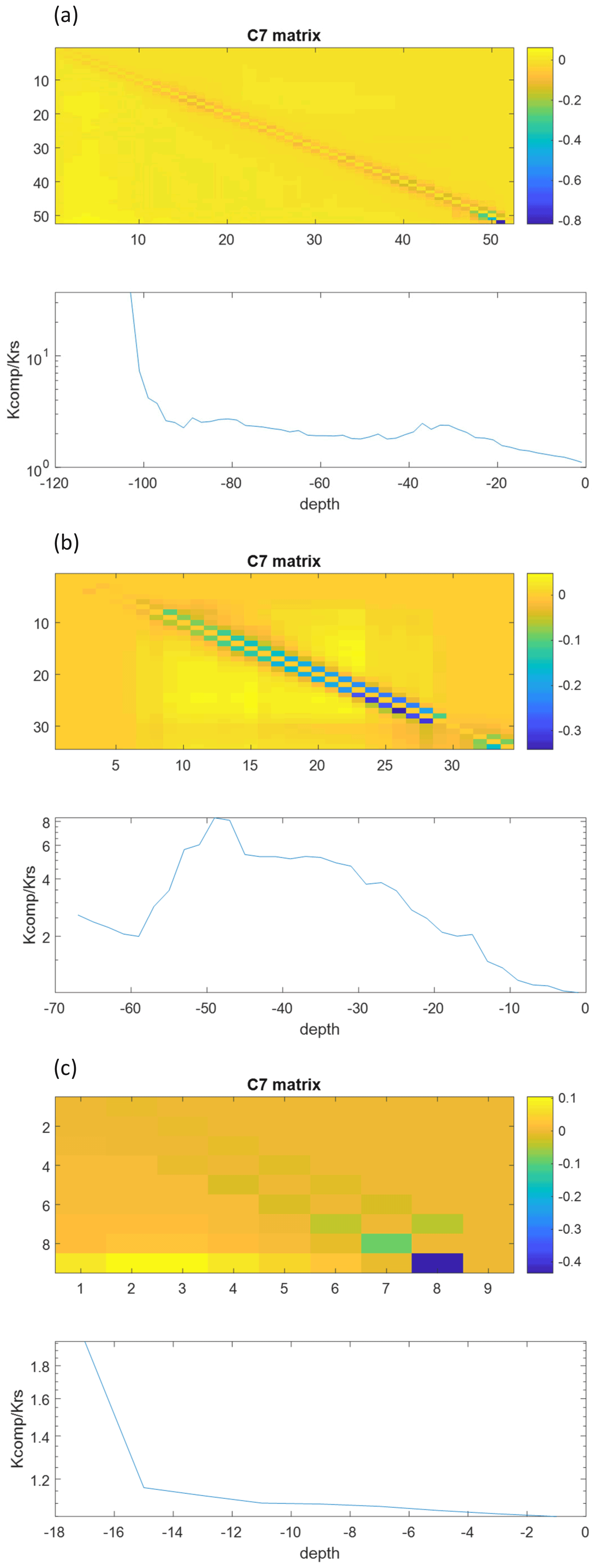
Figure 11C7 matrices and ratios of of the exact model for the maize (a), sunflower (b), and grass (c) root systems.
We analyzed the equation that describes water flow in a network of root segments, which constitutes a root system architecture (RSA) and reformulated it into a form that lends itself to upscaling and to deriving simpler or parsimonious root water uptake models.
In line with Couvreur et al. (2012), we deduced that the total uptake by a root system is a simple function of a weighted soil water hydraulic head, and the weights are equal to the water uptake by the RSA in a uniform soil water hydraulic head field. The root system conductance, Krs, and the uptake distribution for uniform soil water hydraulic head, i.e., the standardized uptake fraction, SUF, are the two properties of the root system that define the relation between the transpiration, the collar hydraulic head, and the distribution of the soil water potentials. This implies that, for any distribution of soil water hydraulic heads that leads to the same weighted hydraulic head, transpiration rate and collar hydraulic head are uniquely related.
We found that the uptake distribution is the sum of the uptake for the case of a uniform soil water hydraulic head, i.e., the weighted hydraulic head, and a correction or compensation term that depends on the difference between the local and weighted soil water hydraulic head. Unlike how it is defined in other approaches (Simunek and Hopmans, 2009; Jarvis, 2011), this compensation term does not depend on the collar hydraulic head or transpiration rate, which is a consequence of the compensation being a passive redistribution process that is not influenced by the transpiration rate as long as the soil water hydraulic heads do not change by the plant water uptake.
When soil water hydraulic heads are assumed to be uniform in certain regions, e.g., in horizontal soil layers, the upscaling of the root water uptake model is trivial and leads to the same form as the detailed model. Whether soil water hydraulic heads remain uniform during root water uptake depends on the spatial distribution of the root segments and on the water redistribution in the soil that cancels out spatial variations in root water uptake (Couvreur et al., 2014a). Further work is needed to evaluate this assumption and to develop upscaling methods when soil water hydraulic heads cannot be assumed to be uniform in the horizontal direction.
The simplified root architectures that are used in land surface models (LSMs) and big root and parallel root models are special cases of RSAs, and the root water uptake models for these architectures can be cast in the same form as the model for a general RSA. For the parallel root model, we could show that the root water uptake model is fully defined by the Krs and SUF of the root system. Krs and SUF of the parallel root system model that is used in a 1D LSM, assuming horizontally uniform soil water hydraulic heads, can be derived directly and exactly from upscaled Krs and SUF of a general root system. The impact of the root segment connections and their root hydraulic properties are directly represented in the Krs and SUF, which can be calculated and scaled up without making any simplifying assumptions about the RSA. The bottom-up approach for parameterizing a parallel root model from 3D RSA models is therefore straightforward. For the big root model, we could not find such a simple relationship, and upscaling was carried out by first deriving the effective conductances of the big root segments based on the intrinsic conductances of the root segments in a certain layer. From the obtained big root model conductances, Krs and SUF were derived. Since the derivation of big root conductances cannot account exactly for the 3D RSA and its hydraulic properties, the obtained Krs and SUF for the big root model are approximations. Another approach that could be pursued is to derive upscaled Krs and SUF directly from the 3D RSA (as was done for the parallel root model) and fit the conductances of the big root model. However, for each layer, only one SUF value is available, whereas two conductances (radial and axial) need to be estimated for the big root segment in that layer. This implies that more information about water uptake by the 3D RSA is required, such as compensatory uptake, in order to parameterize the big root model conductances. The big root model lends itself less to a bottom-up parameterization approach than the parallel root model. Krs and SUF of the parallel root model could also be estimated following a top-down approach from intrinsic root segment conductances without solving the 3D RSA model. But, then it needs to be assumed that the axial root segment conductances are large so that they do not limit the uptake. This assumption led, for the considered root segment hydraulic properties, to an overestimation of the uptake by the distal parts of the roots.
When the exact Krs and SUF are used in the parallel root system model, the approximations in the parallel root system model lead to an underestimation of redistribution of the water uptake for non-uniform distributions of the soil water hydraulic head. However, the typical distribution of radial conductances along a root with lower radial conductances in older more proximal root segments than in younger distal segments that result from aging of root tissues make that the underestimation of the root water uptake redistribution by the parallel root system model is not so important. Even the redistribution of the uptake along a single long root with age-dependent root segment conductances can be represented well with a parallel root system model that uses the exact Krs and SUF. The big root model overestimates the root water uptake redistribution. But, the estimated root water uptake profiles by this model seem to be affected more by the approximate estimation of Krs and SUF from the root segment hydraulic properties. We, therefore, conclude that bottom-up approaches that start from 3D root architecture models and that use age-dependent and/or root-order-dependent hydraulic properties of root segments are promising approaches for parameterizing root water uptake modules of LSMs or crop models. This approach is more reliable than the top-down approach that starts from an upscaled root water uptake model (big root or parallel root model) and derives the effective parameters of these models from root segment hydraulic properties. Since we used information about root segment hydraulic properties and their orientation, the top-down estimated parameters will deviate even more from the correct parameters when proxies of the hydraulic RSA, which are mostly limited to root length density distributions, are used. An often-used argument against RSA models and the proposed bottom-up approach is that they require a lot of input parameters which are hardly available. Indeed, root density distributions are mostly the only information that is available about the RSA. However, root distributions could be used to constrain parameters (Garré et al., 2012; Vansteenkiste et al., 2014) or parameters groups (Pages et al., 2012; Morandage et al., 2019) of RSA models. When information about distributions of root types with depth is available, this information could also be used to parameterize root architecture models, which provides additional information about the distribution of root segment hydraulic properties when different root types can be associated with different hydraulic properties (De Bauw et al., 2020). Since root architecture models also simulate root growth, they provide information about root segment age, which is related to root hydraulic properties and how they change over time. Root growth, but also decay, can be modeled as a function of soil properties and soil conditions (e.g., water content) so that the adaptation of root systems to environmental conditions and two-way feedbacks between root system dynamics and soil water content could be represented (Somma et al., 1998). Next to the RSA architecture, also information about the root segment hydraulic properties is required. Overviews of hydraulic properties of different crops, herbaceous species, and trees are given in Bouda et al. (2018) and Draye et al. (2010). But, variations in root hydraulic properties between different root orders or with root age can be very large (Rewald et al., 2011). Root segment hydraulic properties could be derived either from direct measurements on root segments (Schneider et al., 2017; Zhu and Steudle, 1991; Meunier et al., 2018b), using information on water fluxes in the soil–plant system (e.g., water contents, collar water hydraulic heads, and stable water isotopes in the soil and plant xylem) in combination with inverse modeling (Rothfuss and Javaux, 2017; Cai et al., 2018; Meunier et al., 2018a; Couvreur et al., 2020), or using anatomical information about root tissues in combination with flow modeling (Couvreur et al., 2018; Heymans et al., 2020). The latter approach implies a further downscaling to tissue and cellular levels, which could be used to characterize the variability in root segment properties efficiently. A framework for such a multi-scale approach is presented in Passot et al. (2019). With stochastic simulations of hydraulic RSAs, the impact of the variability in root segment properties on root-system-scale properties and upscaled root water uptake could be derived using the approach presented in this paper.
The uptake profiles and their approximations by the simplified models were calculated for a given non-uniform soil water hydraulic head distribution. Even though the approximations of the uptake profiles are very good, it still requires testing how this evolves over time and affects the dynamics of root water uptake.
The upscaled root water uptake model was derived for a RSA of a single plant or species. The uptake by several plants from the same or from different species of which the roots share the same soil profile with the same Hsoil could be represented by summing up the uptake profiles of the individual plants. When the uptake can be described by a parallel root model, Eq. (22), the uptake by a mixture of plants can also be described by an equivalent parallel root model when the SUFs of the different plants are the same. From Eq. (22), it follows that the equivalent Krs for the mixture corresponds with the sum of the Krs values of the individual plants and the equivalent collar hydraulic head with the Krs weighted Hcollar of the different plants. The joint distribution of Krs and Hcollar or of Krs and the plant transpiration are required to calculate this weighted mean. For a mixture of plants with a different SUF, it is not possible to derive such an equivalent parallel root model that describes the root water uptake profile of the mixture. In that case, the root water uptake profile should be calculated separately for each species or “plant functional” type which is characterized by a specific SUF.
In the current study, we considered a linear flow model in the root system (i.e., root segment hydraulic conductances are not a function of the water pressure heads). Cavitation in the root xylem or changes in radial conductances due to, for instance, aquaporin activation are not considered. Since we focused on the root system hydraulic architecture, we did not consider water potential gradients in the rhizosphere between the bulk soil and the soil–root interface. These gradients can be important and generate an additional non-linear resistance to radial flow. It is still debated whether root xylem cavitation or rhizosphere resistance triggers the non-linear system behavior, but there seems to be more and more evidence that rhizosphere properties trigger the non-linear behavior of the soil–root system (Carminati et al., 2020). Most root water uptake modules that consider root hydraulics in LSMs already include non-linear rhizosphere resistances. How the root water uptake model and its upscaled and simplified versions that are based on a bottom-up analysis of the hydraulic root architecture can be coupled with approaches that consider non-linear resistances to radial flow in the soil (e.g., Gardner and Ehlig, 1962; Hillel et al., 1976; de Jong van Lier et al., 2008, 2013) requires further research. Different proposals were made and implemented by Couvreur et al. (2014b) and Meunier et al. (2018a), but a crucial aspect is how these approaches can be scaled up to 1D models. The non-linearities render the diagonal conductivity matrix diag(K) a function of the hydraulic heads Hcollar, Hx, and Hsoil. This implies that the full set of (non-linear) equations must be solved iteratively to derive “exact” upscaled root system properties, Krs, SUF every time Hcollar, Hx, and Hsoil change. For large root systems, this approach would be unfeasible so that approximations are required. One approach would be to derive functional relations between the upscaled properties and hydraulic head distributions, root and soil hydraulic properties, and root architectures based on a large set of simulations and advanced data analytics. Another approach would be to start with simplifying assumptions that reduce the complexity of the system. A simplification that we are currently testing exploits the linear behavior of the root hydraulics for upscaling RSA first, using the approach developed in this paper, and couples the upscaled equations subsequently to a non-linear rhizosphere flow model.
For a given root node i in the discretized root network, the mass balance is as follows:
where prox(i) represents the proximal (closer to the collar) node of the segment connected to node i, and distal(i) is the distal (further from the collar) node of a segment that is connected to i. Note that Hx[prox(i)] may also be Hcollar when node i is connected to the root collar. The flow from a soil node i to xylem node i is as follows:
The flow from the collar node is the transpiration rate T is as follows:
When we define dH[i] as the difference between the pressure head of node i, which can also be a soil node, and its proximal node (note that each node is connected to only one proximal node, except the collar which has no proximal node), then it follows that:
where IM is the incidence matrix. The differences in pressure heads dH can be expressed as follows:
Plugging Eq. (A5) in (A4) leads to Eq. (4).
When the transpiration T and Hsoil are known, Hcollar and Hx can be obtained by solving the first Nroot+1 equations of Eq. (4). Alternatively, Hcollar can be obtained directly from Eq. (6). From Hcollar and Hsoil, Hx can be derived from solving the second to the Nroot+1 equations in Eq. (4). The xylem hydraulic heads are obtained from the following:
where
Note that C2 and C3 are symmetric matrices.
We can write the fluxes using the lower part of the C matrix as follows:
This can be written out as follows:
where
Working out Eq. (A7), it is found that all entries in CL1 are 0, , and CL3=diag(Kr), so that Eq. (A12) corresponds with the following:
which is the matrix form of Eq. (A2). Plugging Eq. (A6) into the general form of Eq. (A12) gives the following:
where
Note that since C2 and C3 are symmetric matrices, C4 is also a symmetric matrix, and C4 and C5 simplify due to the simple forms of CL1, CL2, and CL3 as follows:
When we consider the case of a uniform soil hydraulic head, Heff, then we can write the following:
When Heff=Hcollar, there is neither flow from the soil to the collar nor flow through the root system from one soil node to the other. From this, it follows that:
If we consider now the total root water uptake, Qtot, which is equal to the transpiration rate, T, then it follows that:
From this, we can derive the root system conductance Krs directly from the following:
The standardized uptake fraction SUF[i], which is defined as the fraction of the uptake by a root node to the total root water uptake under uniform soil water hydraulic head, is related to the matrix C4 and vector C5 as follows:
So, we can write the following for uniform soil water hydraulic heads:
For the general case that the soil water hydraulic heads are not uniform, we can define the effective soil water hydraulic head, Heff, as follows:
After adding and subtracting C5Heff=Krs SUF Heff=Krs SUF⋅SUFTHsoil in Eq. (A17), we obtain the following equation for the root water uptake Q:
From the definitions of C6, C4, SUF, and Krs, it follows that the sum of the elements in the rows of C6 is zero for all rows. This implies that when C6 is multiplied with a Nroot×1 vector with constant elements, a zero vector is obtained. Therefore, we can reformulate the equation for the root water uptake as follows:
Since SUFTHsoil=Heff, and since the sum of all elements in SUF is one so that SUFTHeff=Heff, it follows also that:
The definition of Heff (Eq. A28) makes the sums of all the fluxes in the second term of Eq. (A31) and in the second term of Eq. (A32) both equal to zero. Indeed, when considering Eq. (A32), we can write the following:
since .
Equations (A31) and (A32) have a similar form to the equation that was proposed by Couvreur et al. (2012) to describe water uptake by a root network. In order to draw the analogy and identify differences between the two approaches, we will discuss the nature of the C6 matrix and how it can be transformed or approximated. From the definition of C6, it also follows that the sum of all the elements in the vector C6(Hsoil−Heff) is zero. Therefore, this vector represents the perturbations of the uptake ΔQ at a certain depth due to the perturbation of the soil water hydraulic head at this depth compared to the uptake when the soil water hydraulic head is uniform in the root zone. When there is no net uptake, i.e., when Heff=Hcollar, then C6(Hsoil−Heff) represents the redistribution water fluxes through the root system due to spatial variations in Hsoil. When we consider now that the soil water hydraulic head around node i is ΔH higher than the hydraulic head in all other nodes, then we can define ΔQ[i]=kcomp[i]ΔH. kcomp[i] represents the compensatory root system conductance to transfer water from node i towards all other nodes when there is a hydraulic head difference between the soil water at node i and the soil water next to all other nodes in the root system. ΔQ[i] and kcomp[i] are related to the C6 matrix and SUF vector as follows:
since
We assume now a root system in which all soil nodes are connected via one radial and one axial resistance to the collar node so that the overall resistance to flow from one soil–root node to the collar is equal to the sum of the axial plus radial resistances. We call this root system the parallel root system. The radial and axial resistances for each soil node can however be different. Also a root system in which there is no resistance to axial flow can be considered as a system in which all soil nodes are connected directly to the root collar. But, it is important to keep in mind that systems with a significant axial root resistance can also be considered, as long as there is a direct connection between the soil node and the root collar without additional intermediate nodes that connect to the soil. For instance, fibrous root systems with only primary roots in which uptake only takes place near the root tip but not at the more basal ends, can also be represented by this root system model. For such a root system, it follows that:
In the same vein, it can be deduced in the following that, for such a parallel root system:
The jth column of the C6 matrix represents to what extent water from the jth node can flow to the other nodes in the system. For a parallel root system in which the flow must pass through the collar node, the flow from node j to node i is proportional to the conductance for the flow from node j to the collar node and hence to SUF[j]. Based on this, we can write the C6 matrix for this root system as follows:
where ones is the Nroot vector of all ones.
Since , it follows that, for a parallel root system:
This implies that we can obtain the following equation to simulate root water uptake for the parallel root system:
which is identical to the equation proposed by Couvreur et al. (2012).
For a general root system, we can rewrite the general equation which takes a similar form to the equation that we obtained for the parallel root system.
For the parallel root system, C7 equals the identity matrix, and Kcomp[i] equals Krs.
The MATLAB scripts and input data of the root architectures that were used to generate the figures in this paper are provided in the Supplement.
The supplement related to this article is available online at: https://doi.org/10.5194/hess-25-4835-2021-supplement.
VC initiated the study on the exact macroscopic representation and upscaling of root water uptake. Model development was done by JV, VC, FM, MJ, and MB and programming was done by JV, VC, and FM. Codes were checked by AS. All authors contributed to the conceptualization of the paper. JV wrote the paper, which was critically reviewed by all co-authors.
The authors declare that they have no conflict of interest.
Publisher's note: Copernicus Publications remains neutral with regard to jurisdictional claims in published maps and institutional affiliations.
We would like to thank the reviewers, whose comments helped us to improve the paper.
This work has partially been funded by the German Research Foundation under Germany's Excellence Strategy (grant no. EXC-2070–390732324–PhenoRob) and in the framework of projects P3 and P24 of the priority programme (no. 2089) of “Rhizosphere spatiotemporal organization – a key to rhizosphere functions”. Valentin Couvreur has been supported by the Belgian National Fund for Scientific Research (FRS-FNRS; grant no. 1208619F), the Interuniversity Attraction Poles Program of the Belgian Science Policy Office (grant no. IAP7/29), and the Communauté française de Belgique-Actions de Recherches Concertées (grant no. ARC16/21-075) and Horizon 2020 projects (EPPN2020 731013 and EMPHASIS PREP 739514). Martin Bouda has been supported by the long-term research development of the Czech Academy of Sciences (project no. RVO 67985939) and of the Czech Ministry of Education (OP RDE; project no. CZ.02.2.69/0.0/0.0/18_070/0009075).
This research has been supported by the Deutsche Forschungsgemeinschaft (grant no. EXC-2070 – 390732324 and priority programme 2089), the Fonds De La Recherche Scientifique – FNRS (grant no. 1208619F), the Belgian Federal Science Policy Office (grant no. IAP7/29), the Horizon 2020 (grant no. EMPHASIS-PREP 739514), the Akademie Věd České Republiky (grant no. RVO 67985939), and the Ministerstvo Životního Prostředí (grant no. CZ.02.2.69/0.0/0.0/18_070/0009075).
The article processing charges for this open-access publication were covered by the Forschungszentrum Jülich.
This paper was edited by Nunzio Romano and reviewed by Mario Putti and one anonymous referee.
Amenu, G. G. and Kumar, P.: A model for hydraulic redistribution incorporating coupled soil-root moisture transport, Hydrol. Earth Syst. Sci., 12, 55–74, https://doi.org/10.5194/hess-12-55-2008, 2008.
Bouda, M.: A Big Root Approximation of Site-Scale Vegetation Water Uptake, J. Adv. Model. Earth Sy., 11, 4597–4613, https://doi.org/10.1029/2019ms001806, 2019.
Bouda, M. and Saiers, J. E.: Dynamic effects of root system architecture improve root water uptake in 1D process-based soil-root hydrodynamics, Adv. Water Resour., 110, 319–334, https://doi.org/10.1016/j.advwatres.2017.10.018, 2017.
Bouda, M., Brodersen, C., and Saiers, J.: Whole root system water conductance responds to both axial and radial traits and network topology over natural range of trait variation, J. Theor. Biol., 456, 49–61, https://doi.org/10.1016/j.jtbi.2018.07.033, 2018.
Cai, G. C., Vanderborght, J., Couvreur, V., Mboh, C. M., and Vereecken, H.: Parameterization of Root Water Uptake Models Considering Dynamic Root Distributions and Water Uptake Compensation, Vadose Zone J., 17, 160125, https://doi.org/10.2136/vzj2016.12.0125, 2018.
Carminati, A., Ahmed, M. A., Zarebanadkouki, M., Cai, G., Lovric, G., and Javaux, M.: Stomatal closure prevents the drop in soil water potential around roots, New Phytol., 226, 1541–1543, https://doi.org/10.1111/nph.16451, 2020.
Couvreur, V., Vanderborght, J., and Javaux, M.: A simple three-dimensional macroscopic root water uptake model based on the hydraulic architecture approach, Hydrol. Earth Syst. Sci., 16, 2957–2971, https://doi.org/10.5194/hess-16-2957-2012, 2012.
Couvreur, V., Vanderborght, J., Beff, L., and Javaux, M.: Horizontal soil water potential heterogeneity: simplifying approaches for crop water dynamics models, Hydrol. Earth Syst. Sci., 18, 1723–1743, https://doi.org/10.5194/hess-18-1723-2014, 2014a.
Couvreur, V., Vanderborght, J., Draye, X., and Javaux, M.: Dynamic aspects of soil water availability for isohydric plants: Focus on root hydraulic resistances, Water Resour. Res., 50, 8891–8906, https://doi.org/10.1002/2014wr015608, 2014b.
Couvreur, V., Faget, M., Lobet, G., Javaux, M., Chaumont, F., and Draye, X.: Going with the Flow: Multiscale Insights into the Composite Nature of Water Transport in Roots, Plant Physiol., 178, 1689–1703, https://doi.org/10.1104/pp.18.01006, 2018.
Couvreur, V., Rothfuss, Y., Meunier, F., Bariac, T., Biron, P., Durand, J.-L., Richard, P., and Javaux, M.: Disentangling temporal and population variability in plant root water uptake from stable isotopic analysis: when rooting depth matters in labeling studies, Hydrol. Earth Syst. Sci., 24, 3057–3075, https://doi.org/10.5194/hess-24-3057-2020, 2020.
Daly, K. R., Tracy, S. R., Crout, N. M. J., Mairhofer, S., Pridmore, T. P., Mooney, S. J., and Roose, T.: Quantification of root water uptake in soil using X-ray computed tomography and image-based modelling, Plant Cell Environ., 41, 121–133, https://doi.org/10.1111/pce.12983, 2018.
De Bauw, P., Mai, T. H., Schnepf, A., Merckx, R., Smolders, E., and Vanderborght, J.: A functional-structural model of upland rice root systems reveals the importance of laterals and growing root tips for phosphate uptake from wet and dry soils, Ann. Bot., 126, 789–806, https://doi.org/10.1093/aob/mcaa120, 2020.
de Jong van Lier, Q., van Dam, J. C., Durigon, A., dos Santos, M. A., and Metselaar, K.: Modeling Water Potentials and Flows in the Soil–Plant System Comparing Hydraulic Resistances and Transpiration Reduction Functions, Vadose Zone J., 12, 1–20,https://doi.org/10.2136/vzj2013.02.0039, 2013.
de Jong van Lier, Q. D., van Dam, J. C., Metselaar, K., de Jong, R., and Duijnisveld, W. H. M.: Macroscopic root water uptake distribution using a matric flux potential approach, Vadose Zone J., 7, 1065–1078, https://doi.org/10.2136/vzj2007.0083, 2008.
Doussan, C., Pages, L., and Vercambre, G.: Modelling of the hydraulic architecture of root systems: An integrated approach to water absorption - Model description, Ann. Bot., 81, 213–223, 1998.
Doussan, C., Pierret, A., Garrigues, E., and Pages, L.: Water uptake by plant roots: II – Modelling of water transfer in the soil root-system with explicit account of flow within the root system - Comparison with experiments, Plant Soil, 283, 99–117, 2006.
Draye, X., Kim, Y., Lobet, G., and Javaux, M.: Model-assisted integration of physiological and environmental constraints affecting the dynamic and spatial patterns of root water uptake from soils, J. Exp. Bot., 61, 2145–2155, https://doi.org/10.1093/jxb/erq077, 2010.
Feddes, R. A., Hoff, H., Bruen, M., Dawson, T., de Rosnay, P., Dirmeyer, O., Jackson, R. B., Kabat, P., Kleidon, A., Lilly, A., and Pitman, A. J.: Modeling root water uptake in hydrological and climate models, B. Am. Meteorol. Soc., 82, 2797–2809, 2001.
Ferguson, I. M., Jefferson, J. L., Maxwell, R. M., and Kollet, S. J.: Effects of root water uptake formulation on simulated water and energy budgets at local and basin scales, Environ. Earth Sci., 75, 316, https://doi.org/10.1007/s12665-015-5041-z, 2016.
Fu, C., Wang, G., Goulden, M. L., Scott, R. L., Bible, K., and G. Cardon, Z.: Combined measurement and modeling of the hydrological impact of hydraulic redistribution using CLM4.5 at eight AmeriFlux sites, Hydrol. Earth Syst. Sci., 20, 2001–2018, https://doi.org/10.5194/hess-20-2001-2016, 2016.
Gardner, W. R. and Ehlig, C. F.: Some Observations on the Movement of Water to Plant Roots, Agron. J., 54, 453–456, https://doi.org/10.2134/agronj1962.00021962005400050024x, 1962.
Garré, S., Pagès, L., Laloy, E., Javaux, M., Vanderborght, J., and Vereecken, H.: Parameterizing a Dynamic Architectural Model of the Root System of Spring Barley from Minirhizotron Data, Vadose Zone J., 11, vzj2011.0179, https://doi.org/10.2136/vzj2011.0179, 2012.
Gayler, S., Ingwersen, J., Priesack, E., Wohling, T., Wulfmeyer, V., and Streck, T.: Assessing the relevance of subsurface processes for the simulation of evapotranspiration and soil moisture dynamics with CLM3.5: comparison with field data and crop model simulations, Environ. Earth Sci., 69, 415–427, https://doi.org/10.1007/s12665-013-2309-z, 2013.
Good, S. P., Noone, D., and Bowen, G.: Hydrologic connectivity constrains partitioning of global terrestrial water fluxes, Science, 349, 175–177, https://doi.org/10.1126/science.aaa5931, 2015.
Gou, S. and Miller, G.: A groundwater-soil-plant-atmosphere continuum approach for modelling water stress, uptake, and hydraulic redistribution in phreatophytic vegetation, Ecohydrology, 7, 1029–1041, https://doi.org/10.1002/eco.1427, 2014.
Heymans, A., Couvreur, V., LaRue, T., Paez-Garcia, A., and Lobet, G.: GRANAR, a Computational Tool to Better Understand the Functional Importance of Monocotyledon Root Anatomy, Plant Physiol., 182, 707–720, https://doi.org/10.1104/pp.19.00617, 2020.
Hillel, D., Talpaz, H., and Vankeulen, H.: Macroscopic-Scale Model of Water Uptake by a Nonuniform Root-System and of Water and Salt Movement in Soil Profile, Soil Sci., 121, 242–255, https://doi.org/10.1097/00010694-197604000-00009, 1976.
Hopmans, J. W. and Bristow, K. L.: Current capabilities and future needs of root water and nutrient uptake modeling, Adv. Agron., 77, 103–183, 2002.
Jarvis, N. J.: Simple physics-based models of compensatory plant water uptake: concepts and eco-hydrological consequences, Hydrol. Earth Syst. Sci., 15, 3431–3446, https://doi.org/10.5194/hess-15-3431-2011, 2011.
Javaux, M., Schröder, T., Vanderborght, J., and Vereecken, H.: Use of a three-dimensional detailed modeling approach for predicting root water uptake, Vadose Zone J., 7, 1079–1088, https://doi.org/10.2136/vzj2007.0115, 2008.
Javaux, M., Couvreur, V., Vanderborght, J., and Vereecken, H.: Root Water Uptake: From Three-Dimensional Biophysical Processes to Macroscopic Modeling Approaches, Vadose Zone J., 12, 1–16, https://doi.org/10.2136/vzj2013.02.0042, 2013.
Katul, G. G. and Siqueira, M. B.: Biotic and abiotic factors act in coordination to amplify hydraulic redistribution and lift, New Phytol., 187, 4–6, 2010.
Kennedy, D., Swenson, S., Oleson, K. W., Lawrence, D. M., Fisher, R., da Costa, A. C. L., and Gentine, P.: Implementing Plant Hydraulics in the Community Land Model, Version 5, J. Adv. Model. Earth Sy., 11, 485–513, https://doi.org/10.1029/2018ms001500, 2019.
Landsberg, J. J. and Fowkes, N. D.: Water Movement Through Plant Roots, Ann. Bot., 42, 493–508, https://doi.org/10.1093/oxfordjournals.aob.a085488, 1978.
Liu, Y., Kumar, M., Katul, G. G., Feng, X., and Konings, A. G.: Plant hydraulics accentuates the effect of atmospheric moisture stress on transpiration, Nat. Clim. Change, 10, 691–695, https://doi.org/10.1038/s41558-020-0781-5, 2020.
Manoli, G., Bonetti, S., Domec, J. C., Putti, M., Katul, G., and Marani, M.: Tree root systems competing for soil moisture in a 3D soil-plant model, Adv. Water Resour., 66, 32–42, https://doi.org/10.1016/j.advwatres.2014.01.006, 2014.
Manoli, G., Huang, C. W., Bonetti, S., Domec, J. C., Marani, M., and Katul, G.: Competition for light and water in a coupled soil-plant system, Adv. Water Resour., 108, 216–230, https://doi.org/10.1016/j.advwatres.2017.08.004, 2017.
Meunier, F., Couvreur, V., Draye, X., Vanderborght, J., and Javaux, M.: Towards quantitative root hydraulic phenotyping: novel mathematical functions to calculate plant-scale hydraulic parameters from root system functional and structural traits, J. Math. Biol., 75, 1133–1170, https://doi.org/10.1007/s00285-017-1111-z, 2017a.
Meunier, F., Couvreur, V., Draye, X., Zarebanadkouki, M., Vanderborght, J., and Javaux, M.: Water movement through plant roots – exact solutions of the water flow equation in roots with linear or exponential piecewise hydraulic properties, Hydrol. Earth Syst. Sci., 21, 6519–6540, https://doi.org/10.5194/hess-21-6519-2017, 2017b.
Meunier, F., Draye, X., Vanderborght, J., Javaux, M., and Couvreur, V.: A hybrid analytical-numerical method for solving water flow equations in root hydraulic architectures, Appl. Math. Model., 52, 648–663, https://doi.org/10.1016/j.apm.2017.08.011, 2017c.
Meunier, F., Rothfuss, Y., Bariac, T., Biron, P., Richard, P., Durand, J. L., Couvreur, V., Vanderborght, J., and Javaux, M.: Measuring and Modeling Hydraulic Lift of Lolium multiflorum Using Stable Water Isotopes, Vadose Zone J., 17, 160134, https://doi.org/10.2136/vzj2016.12.0134, 2018a.
Meunier, F., Zarebanadkouki, M., Ahmed, M. A., Carminati, A., Couvreur, V., and Javaux, M.: Hydraulic conductivity of soil-growth lupine and maize unbranched roots and maize root-shoot junctions, J. Plant Physiol., 227, 31–44, https://doi.org/10.1016/j.jplph.2017.12.019, 2018b.
Morandage, S., Schnepf, A., Leitner, D., Javaux, M., Vereecken, H., and Vanderborght, J.: Parameter sensitivity analysis of a root system architecture model based on virtual field sampling, Plant Soil, 438, 101–126, https://doi.org/10.1007/s11104-019-03993-3, 2019.
Nguyen, T. H., Langensiepen, M., Vanderborght, J., Hüging, H., Mboh, C. M., and Ewert, F.: Comparison of root water uptake models in simulating CO2 and H2O fluxes and growth of wheat, Hydrol. Earth Syst. Sci., 24, 4943–4969, https://doi.org/10.5194/hess-24-4943-2020, 2020.
Nimah, M. N. and Hanks, R. J.: Model for Estimating Soil Water, Plant, and Atmospheric Interrelations: I. Description and Sensitivity, Soil Sci. Soc. Am. J., 37, 522–527, https://doi.org/10.2136/sssaj1973.03615995003700040018x, 1973.
Oki, T. and Kanae, S.: Global Hydrological Cycles and World Water Resources, Science, 313, 1068–1072, https://doi.org/10.1126/science.1128845, 2006.
Pages, L., Bruchou, C., and Garre, S.: Links Between Root Length Density Profiles and Models of the Root System Architecture, Vadose Zone J., 11, vzj2011.0152, https://doi.org/10.2136/vzj2011.0152, 2012.
Passot, S., Couvreur, V., Meunier, F., Draye, X., Javaux, M., Leitner, D., Pagès, L., Schnepf, A., Vanderborght, J., and Lobet, G.: Connecting the dots between computational tools to analyse soil-root water relations, J. Exp. Bot., 70, 2345–2357, https://doi.org/10.1093/jxb/ery361, 2019.
Quijano, J. C. and Kumar, P.: Numerical simulations of hydraulic redistribution across climates: The role of the root hydraulic conductivities, Water Resour. Res., 51, 8529–8550, https://doi.org/10.1002/2014wr016509, 2015.
Quijano, J. C., Kumar, P., Drewry, D. T., Goldstein, A., and Misson, L.: Competitive and mutualistic dependencies in multispecies vegetation dynamics enabled by hydraulic redistribution, Water Resour. Res., 48, W05518, https://doi.org/10.1029/2011wr011416, 2012.
Quijano, J. C., Kumar, P., and Drewry, D. T.: Passive regulation of soil biogeochemical cycling by root water transport, Water Resour. Res., 49, 3729–3746, https://doi.org/10.1002/wrcr.20310, 2013.
Rewald, B., Ephrath, J. E., and Rachmilevitch, S.: A root is a root is a root? Water uptake rates of Citrus root orders, Plant Cell Environ., 34, 33–42, https://doi.org/10.1111/j.1365-3040.2010.02223.x, 2011.
Roose, T. and Fowler, A. C.: A model for water uptake by plant roots, J. Theor. Biol., 228, 155–171, https://doi.org/10.1016/j.jtbi.2003.12.012, 2004.
Rothfuss, Y. and Javaux, M.: Reviews and syntheses: Isotopic approaches to quantify root water uptake: a review and comparison of methods, Biogeosciences, 14, 2199–2224, https://doi.org/10.5194/bg-14-2199-2017, 2017.
Ryel, R. J., Caldwell, M. M., Yoder, C. K., Or, D., and Leffler, A. J.: Hydraulic redistribution in a stand of Artemisia tridentata: evaluation of benefits to transpiration assessed with a simulation model, Oecologia, 130, 173–184, https://doi.org/10.1007/s004420100794, 2002.
Schneider, H. M., Wojciechowski, T., Postma, J. A., Brown, K. M., Lücke, A., Zeisler, V., Schreiber, L., and Lynch, J. P.: Root cortical senescence decreases root respiration, nutrient content and radial water and nutrient transport in barley, Plant Cell Environ., 40, 1392–1408, https://doi.org/10.1111/pce.12933, 2017.
Schnepf, A., Leitner, D., Landl, M., Lobet, G., Mai, T. H., Morandage, S., Sheng, C., Zorner, M., Vanderborght, J., and Vereecken, H.: CRootBox: a structural-functional modelling framework for root systems, Ann. Bot., 121, 1033–1053, https://doi.org/10.1093/aob/mcx221, 2018.
Simunek, J. and Hopmans, J. W.: Modeling compensated root water and nutrient uptake, Ecol. Model., 220, 505–521, https://doi.org/10.1016/j.ecolmodel.2008.11.004, 2009.
Siqueira, M., Katul, G., and Porporato, A.: Onset of water stress, hysteresis in plant conductance, and hydraulic lift: Scaling soil water dynamics from millimeters to meters, Water Resour. Res., 44, W01432, https://doi.org/10.1029/2007wr006094, 2008.
Somma, F., Hopmans, J. W., and Clausnitzer, V.: Transient three-dimensional modeling of soil water and solute transport with simultaneous root growth, root water and nutrient uptake, Plant Soil, 202, 281–293, 1998.
Sulis, M., Couvreur, V., Keune, J., Cai, G., Trebs, I., Junk, J., Shrestha, P., Simmer, C., Kollet, S. J., Vereecken, H., and Vanderborght, J.: Incorporating a root water uptake model based on the hydraulic architecture approach in terrestrial systems simulations, Agr. Forest Meteorol., 269–270, 28–45, https://doi.org/10.1016/j.agrformet.2019.01.034, 2019.
Tang, J. Y., Riley, W. J., and Niu, J.: Incorporating root hydraulic redistribution in CLM4.5: Effects on predicted site and global evapotranspiration, soil moisture, and water storage, J. Adv. Model. Earth Sy., 7, 1828–1848, https://doi.org/10.1002/2015ms000484, 2015.
Trenberth, K. E., Smith, L., Qian, T., Dai, A., and Fasullo, J.: Estimates of the Global Water Budget and Its Annual Cycle Using Observational and Model Data, J. Hydrometeorol., 8, 758–769, https://doi.org/10.1175/jhm600.1, 2007.
Vansteenkiste, J., Van Loon, J., Garre, S., Pages, L., Schrevens, E., and Diels, J.: Estimating the parameters of a 3-D root distribution function from root observations with the trench profile method: case study with simulated and field-observed root data, Plant Soil, 375, 75–88, https://doi.org/10.1007/s11104-013-1942-3, 2014.
Vereecken, H., Huisman, J. A., Franssen, H. J. H., Bruggemann, N., Bogena, H. R., Kollet, S., Javaux, M., van der Kruk, J., and Vanderborght, J.: Soil hydrology: Recent methodological advances, challenges, and perspectives, Water Resour. Res., 51, 2616–2633, https://doi.org/10.1002/2014wr016852, 2015.
Vereecken, H., Schnepf, A., Hopmans, J. W., Javaux, M., Or, D., Roose, T., Vanderborght, J., Young, M. H., Amelung, W., Aitkenhead, M., Allison, S. D., Assouline, S., Baveye, P., Berli, M., Brüggemann, N., Finke, P., Flury, M., Gaiser, T., Govers, G., Ghezzehei, T., Hallett, P., Hendricks Franssen, H. J., Heppell, J., Horn, R., Huisman, J. A., Jacques, D., Jonard, F., Kollet, S., Lafolie, F., Lamorski, K., Leitner, D., McBratney, A., Minasny, B., Montzka, C., Nowak, W., Pachepsky, Y., Padarian, J., Romano, N., Roth, K., Rothfuss, Y., Rowe, E. C., Schwen, A., Šimůnek, J., Tiktak, A., Van Dam, J., van der Zee, S. E. A. T. M., Vogel, H. J., Vrugt, J. A., Wöhling, T., and Young, I. M.: Modeling Soil Processes: Review, Key Challenges, and New Perspectives, Vadose Zone J., 15, 1–57, https://doi.org/10.2136/vzj2015.09.0131, 2016.
Whitley, R., Beringer, J., Hutley, L. B., Abramowitz, G., De Kauwe, M. G., Evans, B., Haverd, V., Li, L., Moore, C., Ryu, Y., Scheiter, S., Schymanski, S. J., Smith, B., Wang, Y.-P., Williams, M., and Yu, Q.: Challenges and opportunities in land surface modelling of savanna ecosystems, Biogeosciences, 14, 4711–4732, https://doi.org/10.5194/bg-14-4711-2017, 2017.
Wilderotter, O.: An adaptive numerical method for the Richards equation with root growth, Plant Soil, 251, 255–267, https://doi.org/10.1023/a:1023031924963, 2003.
Wöhling, T., Gayler, S., Priesack, E., Ingwersen, J., Wizemann, H.-D., Högy, P., Cuntz, M., Attinger, S., Wulfmeyer, V., and Streck, T.: Multiresponse, multiobjective calibration as a diagnostic tool to compare accuracy and structural limitations of five coupled soil-plant models and CLM3.5, Water Resour. Res., 49, 8200–8221, https://doi.org/10.1002/2013WR014536, 2013.
Yan, B. Y. and Dickinson, R. E.: Modeling hydraulic redistribution and ecosystem response to droughts over the Amazon basin using Community Land Model 4.0 (CLM4), J. Geophys. Res.-Biogeosci., 119, 2130–2143, https://doi.org/10.1002/2014jg002694, 2014.
Zarebanadkouki, M., Meunier, F., Couvreur, V., Cesar, J., Javaux, M., and Carminati, A.: Estimation of the hydraulic conductivities of lupine roots by inverse modelling of high-resolution measurements of root water uptake, Ann. Bot., 118, 853–864, https://doi.org/10.1093/aob/mcw154, 2016.
Zhu, G. L. and Steudle, E.: Water Transport across Maize Roots, Simultaneous Measurement of Flows at the Cell and Root Level by Double Pressure Probe Technique, Plant Physiol., 95, 305–315, https://doi.org/10.1104/pp.95.1.305, 1991.
Zhu, S. G., Chen, H. S., Zhang, X. X., Wei, N., Wei, S. G., Yuan, H., Zhang, S. P., Wang, L. L., Zhou, L. H., and Dai, Y. J.: Incorporating root hydraulic redistribution and compensatory water uptake in the Common Land Model: Effects on site level and global land modeling, J. Geophys. Res.-Atmos., 122, 7308–7322, https://doi.org/10.1002/2016jd025744, 2017.