the Creative Commons Attribution 4.0 License.
the Creative Commons Attribution 4.0 License.
 | 06 Sep 2021
A study on the drag coefficient in wave attenuation by vegetation
Bensheng Huang
Chao Tan
Xiangju Cheng
Vegetation in wetlands is a large-scale nature-based resource providing a myriad of services for human beings and the environment, such as dissipating incoming wave energy and protecting coastal areas. For understanding wave height attenuation by vegetation, there are two main traditional calibration approaches to the drag effect acting on the vegetation. One of them is based on the rule that wave height decays through the vegetated area by a reciprocal function and another by an exponential function. In both functions, the local wave height reduces with distance from the beginning of the vegetation depending on damping factors. These two damping factors, which are usually obtained from calibration by measured local wave height, are linked to the drag coefficient and measurable parameters, respectively. So the drag coefficient that quantifies the effect of the vegetation can be calculated by different methods, followed by connecting this coefficient to hydraulic parameters to make it predictable. In this study, two relations between these two damping factors and methods to calculate the drag coefficient have been investigated by 99 laboratory experiments. Finally, relations between the drag coefficient and relevant hydraulic parameters were analyzed. The results show that emergent conditions of the vegetation should be considered when studying the drag coefficient; traditional methods which had overlooked this condition cannot perform well when the vegetation was emerged. The new method based on the relation between these two damping factors performed as well as the well-recognized method for emerged and submerged vegetation. Additionally, the Keulegan–Carpenter number can be a suitable hydraulic parameter to predict the drag coefficient and only the experimental setup, especially the densities of the vegetation, can affect the prediction equations.
- Article
(2486 KB) - Full-text XML
- BibTeX
- EndNote


To meet the current wave prevention requirements, it is practical to construct ecological safety barriers with wetland vegetation based on natural conditions. Vegetation in wetlands can enhance the toughness of the coast and save construction investment effectively by dissipating incoming wave energy (Reguero et al., 2018). Practice also has proved that vegetation in wetlands can provide services such as enhancing the coastal ecosystem and biodiversity, enhancing fisheries and forestry production, increasing bank stability, and promoting tourism economy, whereas the vegetated area occupies land resources in the floodplain (Schaubroeck, 2017; Keesstra, 2018). Hence, it is necessary to better understand the mechanism of wave attenuation to promote the efficiency of the nature-based solution.
Wave attenuation by vegetation is mainly induced by the drag force provided by the vegetation acting on water motion, as investigated in different research topics such as numerical modeling (e.g., Wu et al., 2016; Suzuki et al., 2019), laboratory experiment (e.g., Hu et al., 2014; Wu and Cox, 2015, 2016), or field study (e.g., Danielsen et al., 2005; Quartel et al., 2007). The drag force is closely related to the drag coefficient CD which quantifies the drag or resistance of vegetation in water (Chen et al., 2018). This coefficient is one of the most uncertain parameters in the complicated interaction between the vegetated area and water, because the drag effect can be fairly different on various time and space scales.
The calibration method for the drag coefficient is based on the perspective of wave energy dissipation and wave height reduction which will be discussed in Sect. 2, while Dean (1979) and Kobayashi et al. (1993) proposed that local wave height decaying through the vegetated area follows a reciprocal function and exponential function, respectively. These two calibration functions describe local wave height with a distance from the beginning of vegetation and a factor reflecting the damping, so the corresponding factor can be calibrated based on measured wave height through the vegetated area. The damping factor α′ from the reciprocal function and the exponential damping factor k′ from the exponential function are often linked to the drag coefficient CD as well as measurable parameters such as water depth and density of stems. For instance, Dean (1979) proposed an equation to calculate CD based on the damping factor, and the model has been developed by researcher teams such as Knutson et al. (1982), Dalrymple et al. (1984), and Losada et al. (2016). Overall, the drag coefficient can be calculated by calibrating α′ or k′ using measured local wave height; then the researchers built nonlinear relations between CD and hydraulic parameters such as the Reynolds number (e.g., Hu et al., 2014; He et al., 2019). In this way, the drag of vegetation in water becomes predictable based on the nonlinear relations and the values of these hydraulic parameters under different operating conditions.
Zhang et al. (2021) compared these two calibration approaches by these two featured functions directly and yielded a connection between α′ and k′; then a new equation to calculate the drag coefficient has been revealed. However, Zhang et al. (2021) overlooked the relation between k′ and CD by Kobayashi et al. (1993) and only used the relation between α′ and CD by Dean (1979). In this article, using the well-documented relation between the damping factor α′ and the drag coefficient CD by Dalrymple et al. (1984), as well as the mentioned relation by Kobayashi et al. (1993), these two traditional approaches have been compared from another perspective, and the second connection between α′ and k′ has been revealed.
Hence, there are two relations between the damping factor and the exponential damping factor from the two perspectives, and they have been analyzed by 99 cases from collected data and experiments in this study. Additionally, in normal tidal conditions and at the initial stage of storm surge, vegetation in wetlands can be emerged, while, by storm surge, vegetation is submerged or nearly submerged. Existing methods to calculate the drag coefficient have been compared considering these emergence conditions. Finally, relations between CD and hydraulic parameters, e.g., the Reynolds number (Re), the Keulegan–Carpenter number (KC), and the Ursell number (Ur), have been studied.
Typically, the drag coefficient CD is determined from the perspective of wave energy dissipation, represented by the decay of wave height. Dean (1979) proposed one of the first models for wave attenuation by vegetation in which wave height throughout the vegetated area can be expressed as a reciprocal function:
where KX (–) is the relative wave height at a distance X (m) through the vegetation field from the beginning of vegetation, H(X) (m) is the local wave height, H0 (m) is the incident wave height, and α′ (m−1) is the damping factor.
Based on empirical estimates of fluid drag forces acting on vertical, rigid cylinders, Dean (1979) found that
where d (m) is the diameter of the circular vegetation cylinder, h (m) is the water depth, and N (stems m−2) is the average number of stems per unit area.
Then Dalrymple et al. (1984) formulated an algebraic dissipation equation practicing linear theory and conservation of wave energy where α′ can be expressed as
where dv (m) is the vegetated area per unit height of plant normal to wave direction, kw (rad m−1) is the wave number, and ls (m) is the submerged stem height.
On the other hand, Kobayashi et al. (1993) published that the local wave height decays exponentially through submerged artificial kelp:
where k′ (m−1) is the exponential damping factor. Based on linear wave theory and the conservation equation of energy, k′ is expressed as the following (Kobayashi et al., 1993):
If we compare these relations between the (exponential) damping factor and the drag coefficient (Eqs. 3 and 5), a relation between the damping factor α′ and the exponential damping factor k′ can be derived:
Recently, Zhang et al. (2021) presented a relation between α′ and k′, looking at these featured functions (Eqs. 1 and 4) directly. This method firstly scaled the distance X:
and
where α ( (–) is the scaled damping factor, L (m) is the length of vegetated area, x () (–) is the scaled distance through the vegetation field, k () (–) is the scaled exponential damping factor, and F(x) and G(x) represent functions.
Then, by using the Taylor expansion, when the scaled distance x equals half, the following equations were derived:
and
where R1(x) and R2(x) are the residual terms. The relative magnitude of each term in Eqs. (9) and (10) has been analyzed by Zhang et al. (2021), and they revealed that the first two terms on the right-hand side of these equations are relatively large compared to other terms. Hence, considering only these two terms in Eqs. (9) and (10), the proportionality results in
which equals
Equations (6) and (12) have built bridges between the exponential function and reciprocal function, verifying that these two functions are reliable and capable to describe the wave height attenuation by vegetation satisfactorily. The rule of the attenuation is then limited by two functions, which can increase the reliability of the calibration.
However, application of Eq. (6) in Eq. (12) results in , which is not appropriate when there is vegetation in the wetlands. Hence, it is worth it to further study the relation between these two damping factors to help us better understand the drag coefficient and wave attenuation by vegetation.
In addition, we had studied the relation between CD and three relevant hydraulic parameters, which are frequently used to model CD, including (1) the Reynolds number, Re (, where ν m2 s−1) is the kinematic viscosity of water and is the maximum horizontal wave velocity from linear wave theory, where T (s) is the wave period; (2) the Keulegan–Carpenter number, KC (, representing oscillatory flow around cylinders; and (3) the Ursell number, Ur (), characterizing the balance between wave steepness and the relative water depth, where λ (m) is the wavelength. Researchers have reported several formulas between CD and Re. For instance, Wu et al. (2011) obtained the following empirical equation:
Besides this, He et al. (2019) revealed that
Hence, the following two formulas are most possible solutions to study the nonlinear relation between CD and these parameters:
where can be Re, KC, or Ur, and a, b, and c are the factors. Values of these factors can be obtained by the regression of CD by calibrated α′ or k′ (Eqs. 3 or 5) and these parameters, and in this way, CD becomes predictable under different operation conditions. We have obtained the values of the factors and the corresponding adjusted R2 as in Sect. 5.4 by both equations, and it is hard to tell the difference between these results from Eqs. (15) and (16). The former was at last chosen because it contains less factors and is simpler than the latter.
The experiments were conducted in a wave flume in Guangdong Key Laboratory of Hydrodynamic Research at Guangdong Research Institute of Water Resources and Hydropower, China. The wave flume is 80.0 m long, 1.8 m wide, and 2.6 m deep (schematized in Fig. 1a, unit: meters). The wave was generated by a wave generator at one end and absorbed at the opposite end.
The start of the vegetated area was located 52.7 m from the wave generator. The uniform vegetation was constructed by putting mimic plants (Fig. 1b) in holes drilled in the bottom. These two heights of mimic plants (lv) were 0.3 and 0.5 m, and dv of the mimic plants was 0.057 m, considering average diameters of the stem and leaves, while the height ratio of them was about 0.5 (Fig. 1b). The three horizontal lengths of the vegetated area (L) were 4, 5, and 6 m, and two mimic stem densities (N) were 25 and 50 stems m−2 (marked as N1 and N2; see Fig. 1c and d). The two water levels of the flume were 0.8 and 1.0 m, so the corresponding water depths of the floodplain (h) were 0.3 and 0.5 m.
The original wave height (Hori) of each designed regular wave was calibrated at 30 m from the wave generator before these tests. In this study, seven wave gages (G1 to G7) were used to measure the wave height time series, which were placed 1 m apart from each other from the beginning of the vegetated area (Fig. 1a), and the measurement at G1 was used as the incident wave height (H0) (Wu and Cox, 2015).
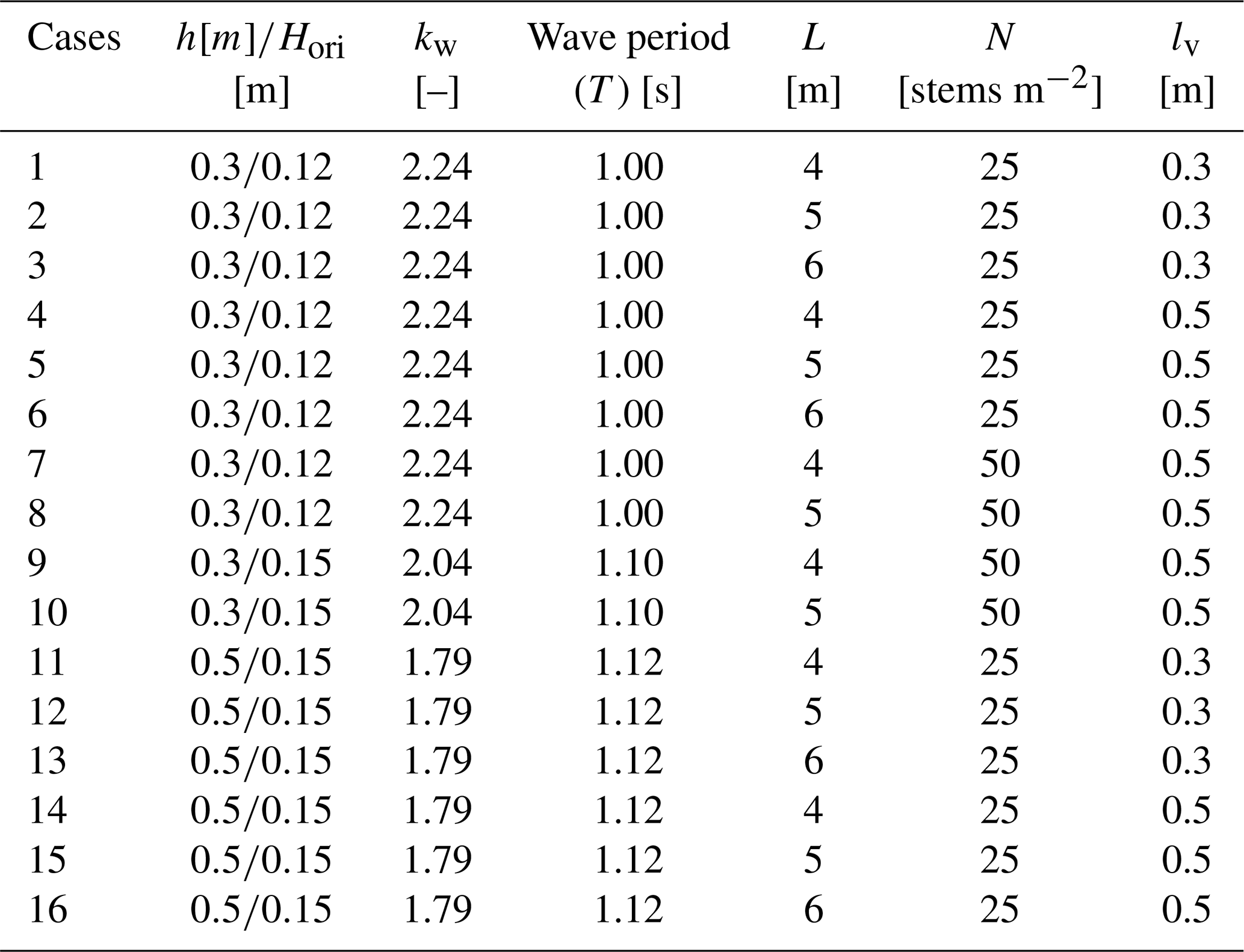
Control tests were carried out with no mimic plants to reduce the influence of flume bed and sidewalls. As listed in Table 1, 16 cases were conducted including various conditions. Data of each test were collected during more than 200 s, and each case was repeated for three times.

Figure 1Experimental setup (unit: meters). (a) Schematic of the wave flume and instrument deployment, when the water depth of the floodplain was 0.5 m and mimic plant's height was 0.5 m; (b) mimic plants with a height of 0.3 m; (c) and (d) top view of the mimic plant canopy with densities of 25 and 50 stems m−2.
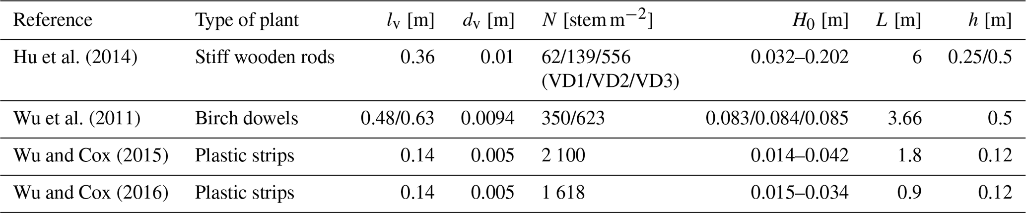
Besides experiments in this study, observations in published literature have been collected from Hu et al. (2014), Wu et al. (2011), and Wu and Cox (2015, 2016) as Zhang et al. (2021) presented. The summarized experimental setup is shown in Table 2. Overall, different laboratory experiments with different operation conditions have been conducted by the research studies.
5.1 Reduction of wave height
Wave height along the vegetated area is a significant index for wave attenuation by vegetation. The calibrated reductions of wave height by three equations demonstrating two examples (cases 13 and 16) are shown in Fig. 2. It is clear that Eqs. (7) and (8) were reliable relations between the scaled distance and the relative wave height. Additionally, with the calibrated k value from Eq. (8), we calculated the value of α according to Eq. (11). Applying the calculated α in Eq. (7), the calculated relative wave height, which was named by Eq. (11) in Fig. 2, was applicable to fit the measurements, which suggested that Eq. (11) is valid. Results also show that the larger the value of the scaled damping factors, the stronger the wave attenuates.
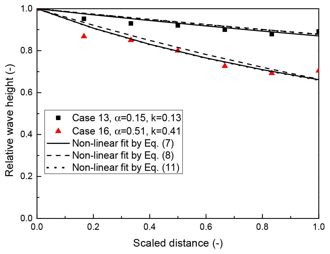
Figure 2Measured and predicted wave attenuation. Square and triangle symbols indicate measurements of cases 13 and 16; solid, dashed, and dotted lines represent the curves fitted by Eqs. (7), (8), and (11), respectively.
5.2 Relation between α and k
The relation between calibrated values of α and k by 99 cases from this study and collected data is shown in Fig. 3. In the study of Wu et al. (2011), Hu et al. (2014), and this research, both submerged and emerged cases have been conducted, and in the study of Wu and Cox (2015, 2016) the vegetation was emerged. The emerged and submerged cases have been separated for studying the influence of the emergent condition (emerged or submerged). Figure 3 shows that there is an obvious relation between α and k for all cases. However, Eq. (6), which was obtained by comparing these relations between the (exponential) damping factor and the drag coefficient by Dalrymple et al. (1984) and Kobayashi et al. (1993), worked well only when values of α and k were smaller than around 0.4. Equation (11), on the other hand, seemed a possible solution for the relation of these two factors, and the relation between α and k is not strongly affected by the emergent condition even though these values are indeed relatively small when the vegetation is submerged (0.04<α<0.56) than when it is emerged (0.12<α<1.43). Notably, the analytical solution by Kobayashi et al. (1993), i.e., Eq. (5), was obtained and conducted using deeply submerged artificial kelp, and H(X)3≅H0H(X)2 was assumed, which can only be valid when wave height reduces slightly through submerged vegetated areas and the exponential damping factor is small. This is why Eq. (6) can only be useful for submerged vegetation.
Equation (11) also revealed that since k is smaller than 2 (Fig. 3). When the vegetation is deeply submerged, the calibrated k is close to zero, and α is larger than but approximately equal to k (Eq. 6); when the vegetation becomes emerged, α and k become relatively large and the difference between them enlarges, which can be seen in Figs. 2 and 3. That is to say, Fig. 3 shows that Eq. (11) works well and it includes Eq. (6) to some extent.
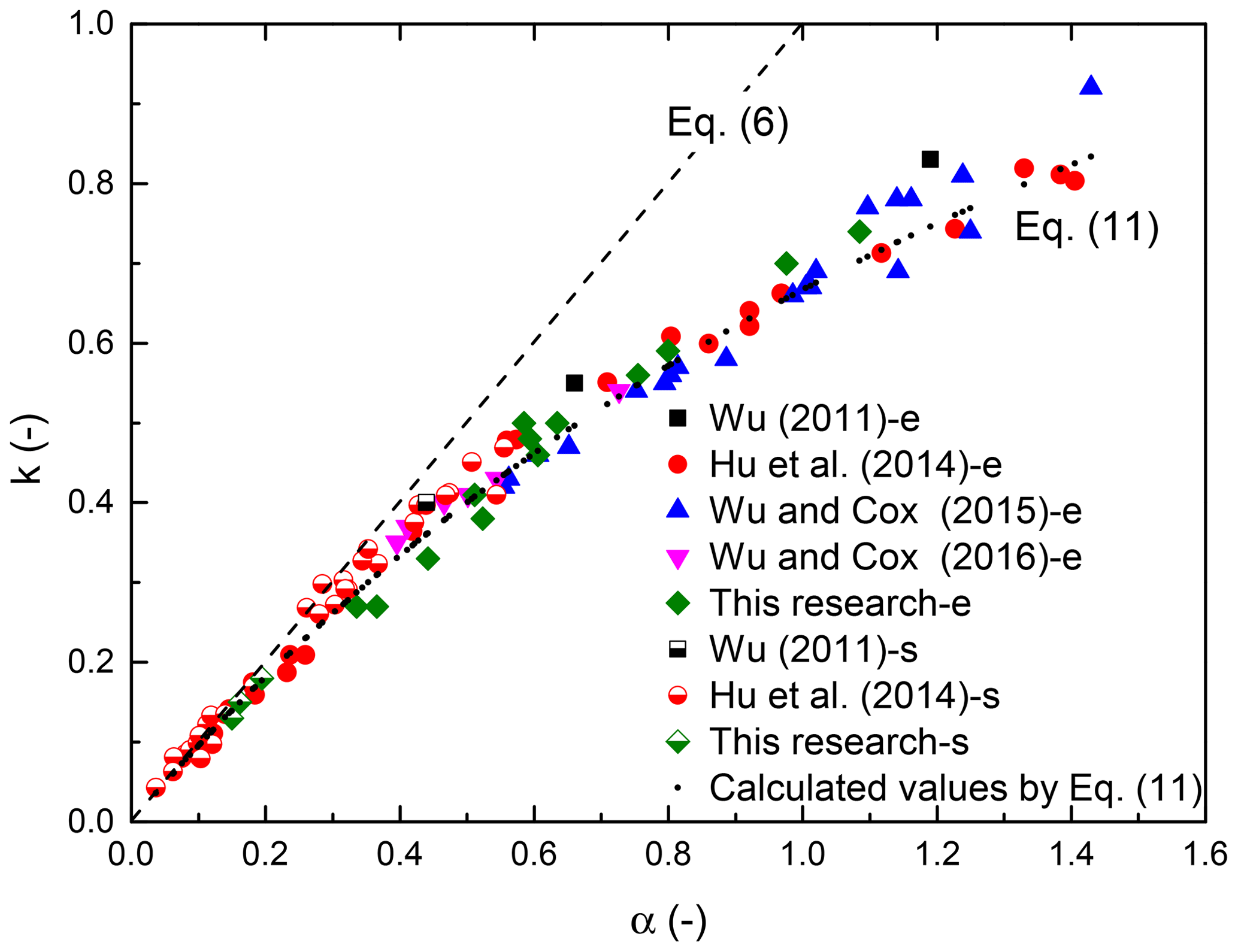
Figure 3Comparison of calibrated α and k. Different symbols indicate cases from different research studies and emergent conditions. For emerged and submerged cases, “-e” and “-s” are added after the references as the legend shows. The dashed and dotted lines indicate calculation by Eqs. (6) and (11), respectively.
5.3 Calculating CD by different methods
5.3.1 Calculating CD by Dean (1979)
Several studies paid attention to the emergent condition of the vegetation recently. This condition (e.g., by ls) has been included in Eq. (3) by Dalrymple et al. (1984), while it had not been considered in Eq. (2) by Dean (1979). Both methods by Dean (1979) and Dalrymple et al. (1984) consider wave height decaying by the reciprocal function, in which the damping factor can be obtained by fitting the local wave height by Eq. (7). In this case, the value of the drag coefficient can be calculated using Eqs. (2) or (3), and the comparison of results by these two equations is shown in Fig. 4. The result shows that these 99 cases obviously can be divided into two categories, and they can be fitted by two linear lines. Both the values of the adjusted R2 of the linear fit of emerged category and submerged category are 0.97, which means the results by these two equations are comparable. However, the slope of the former is about twice as large as the latter, so the emergent condition is necessary to consider when calculating the drag coefficient in wave attenuation by vegetation. Additionally, the linear fit of the submerged category is close to the 1:1 line, which means both equations are reliable and applicable for this category, while one of them is not suitable for emerged category considering the slope of the linear line. Since Eq. (3) pays attention to the emergent condition, it is then regarded as a more satisfactory solution to calculate the drag coefficient for different conditions, while for emerged cases Eq. (2) can lead to larger values.

Figure 4Comparison of the calculated values of CD by Eqs. (3) and (2). Different symbols indicate cases from different research studies, and partially and fully solid symbols denote submerged and emerged cases, respectively. The solid and dashed-dotted lines indicate linear fits of emerged and submerged categories.
5.3.2 Calculating CD by Kobayashi et al. (1993)
Equation (5) by Kobayashi et al. (1993) also considered the emergent condition, and it was obtained by using local wave height decaying exponentially. Hence, in this part, the comparison of the values of the drag coefficient by Eqs. (3) and (5) was studied to learn the influence of different decaying functions, and the result is shown in Fig. 5. The value of CD by Kobayashi et al. (1993) was obtained by calculating CD using Eq. (5) on the basis of the calibrated exponential damping factor by fitting the local wave height using Eq. (8). Figure 5 reveals that CD by Eq. (5) is always smaller than CD by Eq. (3). Also, cases can be divided into two categories. For submerged cases, the drag coefficient by Eq. (5) is close to but slightly smaller than that by Eq. (3), with a slope of 0.96 in Fig. 5; for emerged cased, the former is smaller than the latter when the drag coefficient is larger. This is consistent with the conclusion in Sect. 5.2 since CD has positive correlation with α and k. In short, for calculating the drag coefficient in wave attenuation by submerged vegetation, both Eqs. (3) and (5) can be the solution. However, for emerged cases, Eq. (5) can lead to underestimated values of the calibrated CD.
Additionally, although the regression of data should not be linear since , which is not a constant, if we obtain CD by calibrating the exponential function for emerged cases, we have a rapid assessment that the value will be approximately 77 % of the needed value. Moreover, the result reveals that . Combining Eq. (12), approximates to 0.46, then KX≈0.63 at the end of the vegetation according to Eqs. (4) and (8). This means that the reduction rate () of the wave height for the emerged cases is about 37 %. Furthermore, if we apply k≈0.46 in Eq. (11), α is about 0.60; then KX≈0.63 according to Eqs. (1) and (7). Values of KX which are close to α and k can be used to assess the wave attenuation by emerged vegetation in a very preliminary way.
Of course, several parameters can affect the drag effect. In this case, certain cases should be considered separately instead of using the result from a regression by all the cases with different operating conditions; then the slope of the comparison between the calculated CD by Eqs. (3) and (5) will be different so the calculated relative wave height will be different.
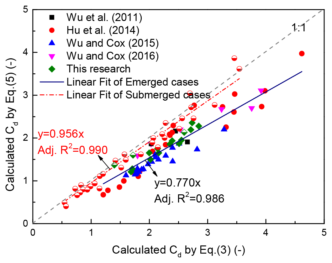
Figure 5Comparison of the calculated values of CD by Eqs. (3) and (5). Details are the same as Fig. 4.
5.3.3 Calculating CD by a new method
The new method obtains the damping factor α′ by using the calibrated k′ based on measured wave height and Eq. (12), so the drag coefficient CD can be calculated by Eq. (3). The Eq. (12)-based method used the rule that the local wave height decays exponentially and the classic relation between the damping factor and CD by Dalrymple et al. (1984). The comparison of the calculated values of CD by Eq. (3) and the new method is shown in Fig. 6. The result shows that there is a strong linear relationship among the calculated values in 99 cases from different research studies. The slope of the linear fit is about unitary, and the adjusted R2 equals 0.99. The result is inspiring and shows that the new method can lead to comparable results to the method by Dalrymple et al. (1984) for the drag coefficient. It is revealed that Eq. (12) is satisfactory and can be a bridge between the damping factor and the exponential damping factor. Based on the results in Figs. 5 and 6, the exponential damping factor k′ can be used to calculate CD while it needs to be converted to α′ based on Eq. (12) instead to be used directly in Eq. (5) for emerged cases; while for submerged cases, it can be a solution to calculate CD directly.

Figure 6Comparison of the calculated values of CD by Eq. (3) and the new method. Different symbols indicate cases from different research studies. The solid line indicates linear fit of all cases.
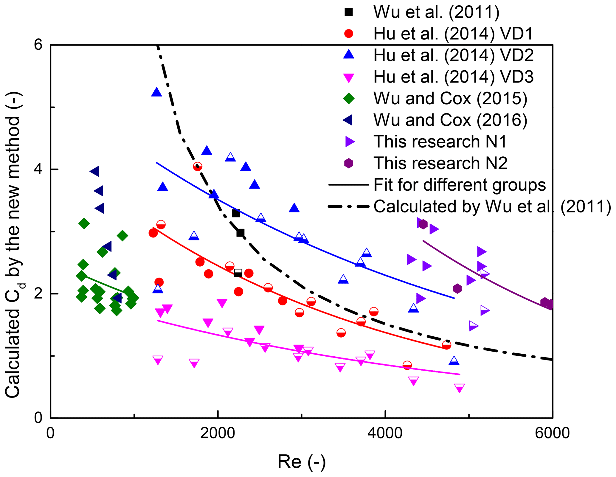
Figure 7Relation between Re and CD by the new method. Different symbols indicate cases from different research studies, and partially and fully solid symbols denote submerged and emerged cases, respectively. The solid lines following groups of the symbols indicate nonlinear fit by Eq. (15).
5.4 Relating CD to Re, KC, and Ur
5.4.1 Relating CD to Re
Relating the calculated CD by calibration method to Re, KC, or Ur is a common method to predict CD. The relation between Re and the calibrated CD by the new method and the nonlinear fit by Eq. (15) are shown in Fig. 7. In the study by Hu et al. (2014) and this research, cases were grouped by different densities. The values of Re ranged from 370 to 38 000, and the solid line following different groups of symbols can basically fit. Results reveal that separating cases from different densities is necessary for studying this relation, while the effect of the emergent condition can be ignorable. Equation (15) was utilized to study this relation, and the outcomes of the factors from nonlinear fit between Re and CD by the new method and by Eq. (3) are shown in Table 3. Results show that values for a certain factor (a or b) based on the new method and Eq. (3) are close to each other, especially for cases from Hu et al. (2014), supporting the fact that the new method is comparable to Dalrymple et al. (1984). Moreover, values of factors can be quite different in various groups in Table 3; hence, laboratory setup could play an important role in the relation between the drag coefficient and the Reynolds number. Hence, this relation is not universal for different cases. For example, the calculated line by Eq. (13) published by Wu et al. (2011) is not very suitable for other groups of measurements. Hence, for engineering applications, case studies are needed for certain issues.
Table 3Outcome of the factors in Eq. (15) between Re and CD by the new method and by Eq. (3).

5.4.2 Relating CD to KC
The relation between KC and CD by the new method is shown in Fig. 8. The values of KC ranged from 9 to 130, and the range is much smaller than that of Re in Fig. 7. Similarly, Eq. (15) was utilized to study the relation between KC and CD, and outcomes of the factors are shown in Table 4. Results show that these fit lines are closer to each other than those in Fig. 7. The adjusted R2 values in Table 4 are overall larger than the corresponding numbers in Table 3. In addition, values for a certain factor based on these two methods are closer to each other than the results in Table 3. From these studied cases, the Keulegan–Carpenter number can be a better parameter to describe the drag coefficient than Re. Besides, for predicting CD by KC, factors in Eq. (15) can be different for different densities of vegetation and operation conditions, but the emergent condition will not affect the result.
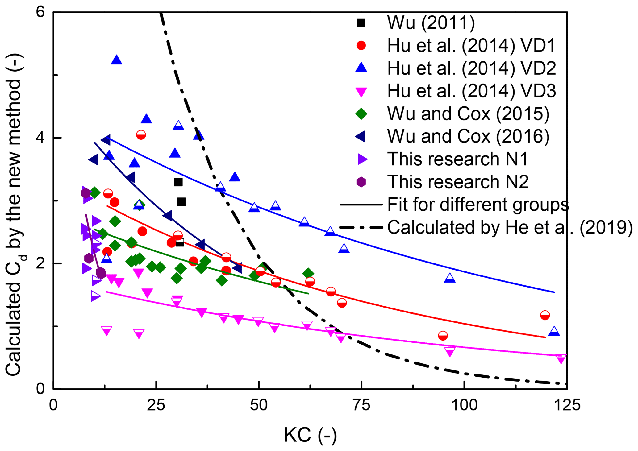
Figure 8Relation between KC and the calculated CD by the new method. Details are the same as Fig. 7.
Table 4Outcome of the factors in Eq. (15) between KC and CD by the new method and by Eq. (3).

5.4.3 Relating CD to Ur
The relation between CD and the Ursell number Ur have also been studied (Fig. 9). The values of Ur ranged from 1 to 68. However, the nonlinear fit by Eqs. (15) is unsatisfactory for all groups since the relation of these data is not so strong. Results show that comparing to Re and KC, Ur is not a well-performed parameter for studying the drag coefficient in wave attenuation by vegetation.
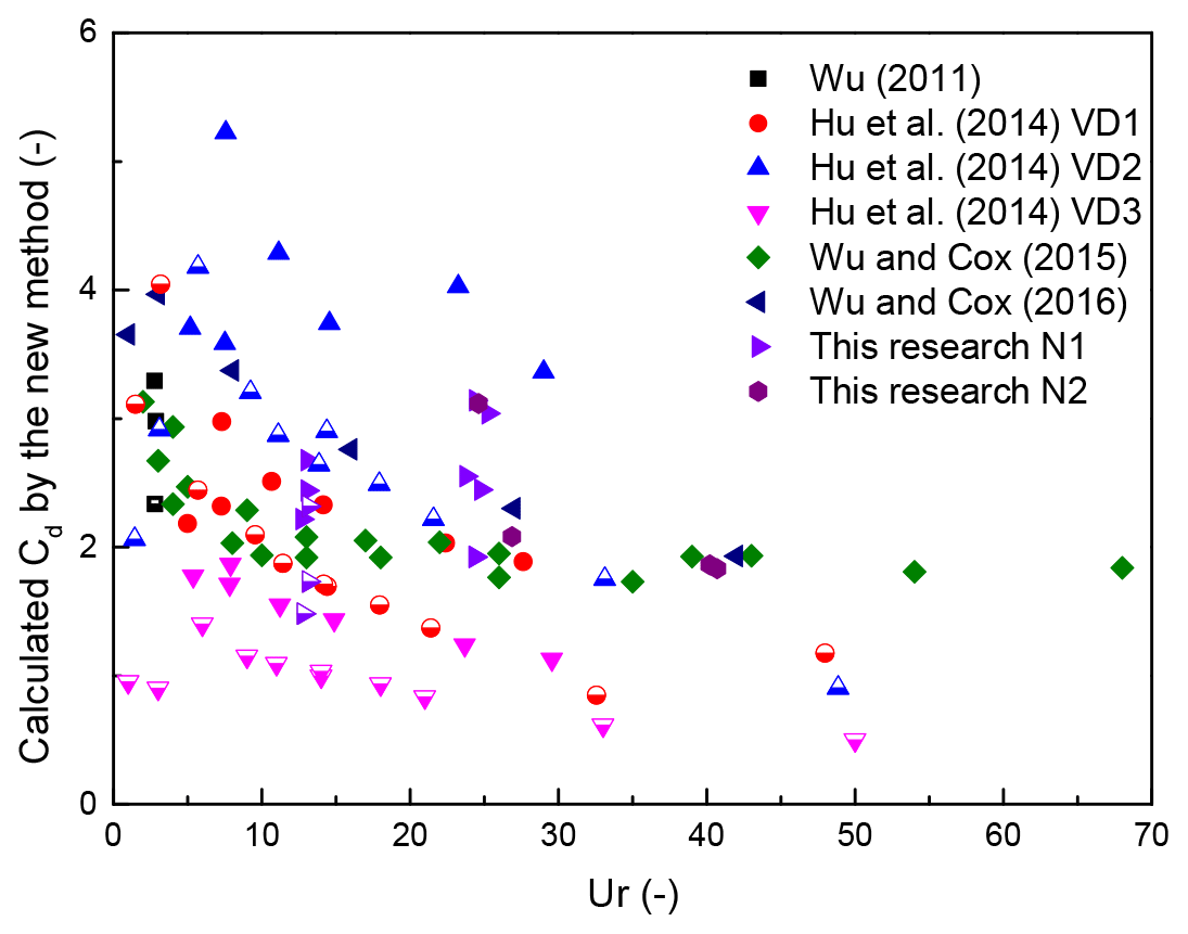
Figure 9Relation between Ur and the calculated CD by the new method. Details are the same as Fig. 7.
Wave attenuation by vegetation in wetlands is a large-scale nature-based solution providing a myriad of services for human beings. For understanding wave attenuation, two main traditional calibration approaches to the drag effect acting on the vegetation have been established, based on local wave height decaying by a reciprocal function or exponential function. These two reliable calibration methods by Dean (1979) and Kobayashi et al. (1993) can be combined from two perspectives: one by combining these featured functions directly (Eqs. 1 and 4) and another by the relations between the (exponential) damping factor and the drag coefficient (Eqs. 3 and 5). So, two relations between the damping factor α′ and the exponential damping factor k′ have been derived (Eqs. 6 and 12). Then, the relation between α′ and k′ and the drag coefficient in wave attenuation were analyzed by 99 laboratory experiments. Furthermore, relations between CD and important hydraulic parameters (Re, KC, and Ur) were analyzed to make CD predictable under certain conditions.
The results showed that the reduction of wave height can be well described by both reciprocal and exponential functions. For submerged vegetation, which reduces wave height relatively slightly, the damping factor approximately equalled the exponential damping factor, and Eq. (6) was applied. However, Eq. (12) was applicable no matter how submerged the vegetation was, which is a satisfactory result. Besides, for submerged vegetation, values of CD calculated with Eq. (2) by Dean (1979) and with Eq. (5) by Kobayashi et al. (1993) were consistent with the well-recognized Eq. (3) by Dalrymple et al. (1984). However, when the vegetation was emerged, Eqs. (2) and (5) were not in line with Eq. (3). On the other hand, the calculated CD values by the new method by Zhang et al. (2021) in combination with Eq. (3) were almost the same as the results from the method by Dalrymple et al. (1984). Additionally, it is appeared that KC performed best to predict CD, better than Re and Ur, although the factors were different in different groups of laboratory observations. Therefore, further studies are needed in a variety of laboratory experiments.
Building a bridge between the two reliable methods by Dean (1979) and Kobayashi et al. (1993) is helpful. In this way, the reduction of wave height is limited by two functions, so experimental outliers can be distinguished. Also, emergent conditions and densities are very significant aspects to study the drag coefficient by vegetation. This method for the drag coefficient have been validated by a great amount of data under different laboratory conditions; however, the interaction between the vegetation and flow field is complicated, and laboratory errors may affect the result, so verification and/or calibration are needed further for predicting the drag coefficient.
The data that support the findings of this study are available from the corresponding author upon reasonable request.
ZZ, BH, and CT did the conceptualization and methodology. ZZ and TC did the data curation and formal analysis. ZZ did validation and visualization. BH and CT did the funding acquisition and project administration. BH and XC did the supervision. All the authors contributed to writing and editing of the article.
The authors declare that they have no conflict of interest.
Publisher’s note: Copernicus Publications remains neutral with regard to jurisdictional claims in published maps and institutional affiliations.
The authors especially thank Zhan Hu and Wei-Cheng Wu for sharing laboratory data.
This work has supported by Guangzhou Science and Technology Program key projects (grant no. 201806010143), the Soft Science Research Program of Guangdong (grant no. 2018B020207004), and the National Key Research and Development Program of China (grant no. 2016YFC0402607).
This paper was edited by Hubert H. G. Savenije and reviewed by two anonymous referees.
Chen, H., Ni, Y., Li, Y., Feng, L., Ou, S., Su, M., Peng, Y., Hu, Z., Uijttewaal, W., and Suzuki, T.: Deriving vegetation drag coefficients in combined wave-current flows by calibration and direct measurement methods, Adv. Water Resour., 122, 217–227, https://doi.org/10.1016/j.advwatres.2018.10.008, 2018.
Dalrymple, R. A., Kirby, J. T., and Hwang, P. A.: Wave diffraction due to areas of energy dissipation, J. Waterw. Port Coast., 110, 67–79, https://doi.org/10.1061/(ASCE)0733-950X(1984)110:1(67), 1984.
Danielsen, F., Sørensen, M. K., Olwig, M. F, Selvam, V., Parish, F., Burgess, N. D., Hiraishi, T., Karunagaran, V. M., Rasmussen, M. S., Hansen, L. B., Quarto, A., and Suryadiputra, N.: The Asian tsunami: a protective role for coastal vegetation, Science, 310, 643, https://doi.org/10.1126/science.1118387, 2005.
Dean, R. G.: Effects of vegetation on shoreline erosional processes, in: Wetland Functions and Values: The State of Our Understanding, MN: American Water Resources Association, Minneapolis, 415–426, 1979.
He, F., Chen, J., and Jiang C.: Surface wave attenuation by vegetation with the stem, root and canopy, Coast. Eng., 152, 103509, https://doi.org/10.1016/j.coastaleng.2019.103509, 2019.
Hu, Z., Suzuki, T., Zitman, T., Uittewaal, W., and Stive, M.: Laboratory study on wave dissipation by vegetation in combined current-wave flow, Coast. Eng., 88, 131–142, https://doi.org/10.1016/j.coastaleng.2014.02.009, 2014.
Keesstra, S., Nunes, J., Novara, A., Finger, D., Avelar, D., Kalantari, Z., and Cerdà, A.: The superior effect of nature based solutions in land management for enhancing ecosystem services, Sci. Total Environ., 610–611, 997–1009, https://doi.org/10.1016/j.scitotenv.2017.08.077, 2018.
Knutson, P. L., Brochu, R. A., Seelig, W. N., and Inskeep, M.: Wave damping in Spartina alterniflora marshes, Wetlands, 2, 87–104, https://doi.org/10.1007/BF03160548, 1982.
Kobayashi, N., Raichle, A. W., and Asano, T.: Wave attenuation by vegetation, J. Waterw. Port Coast., 119, 30–48, https://doi.org/10.1061/(ASCE)0733-950X(1993)119:1(30), 1993.
Losada, I. J., Maza, M., and Lara, J.L.: A new formulation for vegetation-induced damping under combined waves and currents, Coast. Eng., 107, 1–13, https://doi.org/10.1016/j.coastaleng.2015.09.011, 2016.
Quartel, S., Kroon, A., Augustinus, P. G. E. F., Van Santen, P. V., and Tri, N. H.: Wave attenuation in coastal mangroves in the Red River Delta, Vietnam, J. Asian Earth. Sci., 29, 576–584, https://doi.org/10.1016/j.jseaes.2006.05.008, 2007.
Reguero, B. G., Beck, M. W., Bresch, D. N., Calil, J., and Meliane, I.: Comparing the cost effectiveness of nature-based and coastal adaptation: A case study from the Gulf Coast of the United States, PLoS One, 13, e0192132, https://doi.org/10.1371/journal.pone.0192132, 2018.
Schaubroeck, T.: Nature-based solutions: sustainable?, Nature, 543, 315, https://doi.org/10.1038/543315c, 2017.
Suzuki, T., Hu, Z., Kumada, K., Phan, L.K., and Zijlema, M.: Non-hydrostatic modeling of drag, inertia and porous effects in wave propagation over dense vegetation fields, Coast. Eng., 149, 49–64, https://doi.org/10.1016/j.coastaleng.2019.03.011, 2019.
Wu, W. M., Ozeren, Y., Wren, D. G., Chen, Q., Zhang, G., Holland, M., Ding, Y., Kuiry, S. N., Zhang, M., Jadhave, R., Chatagnier, J., Chen, Y., and Gordji, L.: Investigation of surge and wave reduction by vegetation, SERRI Report 80037-01, Southeast Region Research Initiative, Oak Ridge National Laboratory, Oak Ridge, Tennessee, USA, 2011.
Wu, W. C. and Cox, D. T.: Effects of wave steepness and relative water depth on wave attenuation by emergent vegetation, Estuar. Coast. Shelf S., 164, 443–450, https://doi.org/10.1016/j.ecss.2015.08.009, 2015.
Wu, W. C. and Cox, D. T.: Effects of vertical variation in vegetation density on wave attenuation, J. Waterw. Port Coast., 142, 04015020, https://doi.org/10.1061/(ASCE)WW.1943-5460.0000326, 2016.
Wu, W. C., Ma, G., and Cox, D. T.: Modeling wave attenuation induced by the vertical density variations of vegetation, Coast. Eng., 112, 17–27, https://doi.org/10.1016/j.coastaleng.2016.02.004, 2016.
Zhang, Z., Huang B., Ji, H., Tian, X., Qiu, J., Tan, C., and Cheng, X.: A rapid assessment method for calculating the drag coefficient in wave attenuation by vegetation, Acta Oceanol. Sin., 40, 30–35, https://doi.org/10.1007/s13131-021-1726-1, 2021.