the Creative Commons Attribution 4.0 License.
the Creative Commons Attribution 4.0 License.
 | 31 Aug 2021
Delineation of dew formation zones in Iran using long-term model simulations and cluster analysis
Nahid Atashi
Dariush Rahimi
Victoria A. Sinclair
Martha A. Zaidan
Anton Rusanen
Henri Vuollekoski
Markku Kulmala
Timo Vesala
Tareq Hussein
Dew is a non-conventional source of water that has been gaining interest over the last two decades, especially in arid and semi-arid regions. In this study, we performed a long-term (1979–2018) energy balance model simulation to estimate dew formation potential in Iran aiming to identify dew formation zones and to investigate the impacts of long-term variation in meteorological parameters on dew formation. The annual average of dew occurrence in Iran was ∼102 d, with the lowest number of dewy days in summer (∼7 d) and the highest in winter (∼45 d). The average daily dew yield was in the range of 0.03–0.14 L m−2 and the maximum was in the range of 0.29–0.52 L m−2. Six dew formation zones were identified based on cluster analysis of the time series of the simulated dew yield. The distribution of dew formation zones in Iran was closely aligned with topography and sources of moisture. Therefore, the coastal zones in the north and south of Iran (i.e., Caspian Sea and Oman Sea), showed the highest dew formation potential, with 53 and 34 L m−2 yr−1, whereas the dry interior regions (i.e., central Iran and the Lut Desert), with the average of 12–18 L m−2 yr−1, had the lowest potential for dew formation. Dew yield estimation is very sensitive to the choice of the heat transfer coefficient. The uncertainty analysis of the heat transfer coefficient using eight different parameterizations revealed that the parameterization used in this study – the Richards (2004) formulation – gives estimates that are similar to the average of all methods and are neither much lower nor much higher than the majority of other parameterizations and the largest differences occur for the very low values of daily dew yield. Trend analysis results revealed a significant (p<0.05) negative trend in the yearly dew yield in most parts of Iran during the last 4 decades (1979–2018). Such a negative trend in dew formation is likely due to an increase in air temperature and a decrease in relative humidity and cloudiness over the 40 years.
- Article
(13888 KB) - Full-text XML
-
Supplement
(530 KB) - BibTeX
- EndNote


Scarcity and continuously increasing demand on freshwater is one of the socioeconomic problems in many countries, especially in arid and semi-arid regions. It is anticipated that two-thirds of the world's population will suffer of freshwater shortage by the year 2025 (Watkins, 2006). In fact, the water crisis will not only be limited to freshwater resources but also will have an extreme impact on agriculture and livestock (Madani Larijani, 2005).
Scientists have also warned that the water shortage will continue further in the coming decades in the Middle East, where water is one of the most valuable and vulnerable natural resources (Mehryar et al., 2015; Ashraf et al., 2019; Bozorg-Haddad et al., 2020). Iran is one of the countries suffering a freshwater shortage and climate change consequences (Karimi et al., 2018; Afshar and Fahimi, 2019; Emami and Koch, 2019; Naderi, 2020). For instance, the annual average rainfall in Iran is about 250 mm (Alizadeh, 2011). Besides that, 65 % of the country is arid, 20 % is semi-arid, and only 15 % has a humid or semi-humid climate. The Iranian annual renewable water resources is currently less than 2000 m3 per capita and with the current population growth rate (∼1.19 %; CIA, 2020), is expected to be reduced to be less than 1000 m3 per capita by 2025 (Madani Larijani, 2005; Moridi, 2017). Therefore, looking for alternative resources of freshwater is a necessity in the arid and semi-arid regions in Iran.
The atmosphere can be considered a huge renewable reservoir of water (i.e., cloud, fog, and water vapor) and enough to meet the needs of every person on the planet (Tu et al., 2018). Dew is a non-conventional atmospheric resource of water, which forms during the phase transition from vapor to liquid (Tomaszkiewicz et al., 2015) or condensation of atmospheric water vapor on surfaces with a temperature below the dew point (Khalil et al., 2016). Although the amount of dew that can be harvested is relatively small, it can enhance water supply in certain climates or regions, particularly in the absence of precipitation (Tomaszkiewicz et al., 2015). Extracting dew water as a sustainable natural phenomenon by means of radiative (or passive) condensers has been gaining interest over the last two decades. Research on radiative condensers started in the early 1960s with a study conducted in Negev Desert by Gindel (1965). Based on studies in different locations worldwide (Table 1), the highest amount of daily dew yield (typically in the range of 0.2–0.6 L m−2 was observed in arid deserts and semi-arid areas (Kidron, 1999; Alnaser and Barakat, 2000; Agam and Berliner, 2006; Sharan et al., 2007a, b; Lekouch et al., 2012; Tomaszkiewicz et al., 2017; Jia et al., 2019; Tuurre et al., 2019). Some regions with humid climates (e.g., coastal areas and islands) showed lower yield (∼0.2–0.4 L m−2) (Sharan, 2005; Clus et al., 2008; Muselli et al., 2002, 2009; Hanisch et al., 2015), and urban environments had the minimum dew yield (∼0.02–0.3 L m−2) (Richards, 2004; Beysens et al., 2006b; Ye et al., 2007; Muskała et al., 2015; Odeh et al., 2017).
Table 1Dew yield from plane radiative condensers in various field campaigns and models.

Despite the importance of dew and its potential especially in dry areas, it has been disregarded from the water budget in Iran (e.g., Esfandiarnejad et al., 2010; Davtalab et al., 2013). There is a lack of dew data in Iran; therefore, we utilized a gridded model (Vuollekoski et al., 2015) and performed simulations covering 40 years (1979–2018) to estimate the potential of dew yield. This model is based on an energy balance similar to models used in previous studies (e.g., Nilsson, 1996; Jacobs et al., 2008; Maestre-Valero et al., 2011; Arias-Torres and Flores-Prieto, 2016; Beysens, 2016) conducted in different environments. Previous studies have demonstrated that energy balance models are able to predict dew yield within a reasonable agreement with measured dew yield and could also be applicable elsewhere. For example, Tomaszkiewicz et al. (2016) applied a dew prediction model that was developed by Beysens (2016), to generate a dew yield atlas for the Mediterranean region (142 stations). The objective of this study is to identify the major dew formation zones in Iran using a long-term model simulation and to investigate the possible impacts of historic changes to the climate over the last 40 years on dew in Iran.
In order to estimate dew collection potential in Iran, we combined a computationally efficient dew formation model with meteorological reanalysis data spanning 40 years. The model simulation results were used to investigate the spatial–temporal variation of dew yield in Iran. In this study, the term “dew yield” refers to the amount of water that can be harvested on a 1 m2 condenser.
2.1 Meteorological input data
The dew formation model (which is described in detail in Sect. 2.2) requires meteorological data as input. In Iran, there are very few stations with long-term observations of all the required meteorological variables. Therefore, instead of driving the dew model with observations, we use ERA-Interim (Berrisford et al., 2011; Dee et al., 2011), which is a meteorological global reanalysis produced by the European Centre for Medium-Range Weather Forecasts (ECMWF). Reanalysis combines a massive number of observations from a number of sources (satellite, radiosondes, aircraft, buoy data, stations, etc.) with a numerical weather prediction model to produce a coherent, long-term gridded dataset of the atmospheric dynamic and thermodynamic state over the whole globe (Tompkins, 2017).
ERA-Interim covers the time period from January 1979 until August 2019, has a native resolution of 0.75∘, which is approximately 80 km, and has 60 model levels in the vertical profile. Here we considered the time period during 1979–2018 and used input data interpolated to a grid resolution of 0.25∘ (∼30 km) over a domain covering all parts of Iran (Fig. 1). This interpolation was done during the download process using standard ECMWF procedures: continuous fields (e.g., temperature and precipitation) were interpolated using bilinear interpolation and discrete fields (e.g., vegetation and soil type) were interpolated using a nearest neighbor approach.

Figure 1A map of Iran illustrating the geographical topography and the domain of the grid points used in the model simulation. Red stars indicate the selected stations for uncertainty analysis.
Similar to all atmospheric reanalysis, ERA-Interim contains two distinct types of fields: analysis fields and forecast fields. The analysis fields were produced by combining a very short-range forecasts and observations to produce the best fit for both. The forecast fields were produced by the numerical forecast model starting from an analysis. In ERA-Interim, the analysis fields were available every 6 h (00:00, 06:00, 12:00, and 18:00 UTC) and the forecast fields were available every 3 h; hence, they can be used to fill in the gaps between the analysis. Furthermore, the forecast fields can be either instantaneous or accumulated over the forecast period.
The variables that are required for the dew formation model are: air temperature (Ta), dew point temperature (DP), wind speed (WS), and short-wave (Rsw) and long-wave solar radiation (Rlw). From ERA-Interim, we extracted the 2 m Ta and DP from both the analysis and the instantaneous forecasts and obtain the short-wave and long-wave surface radiation as accumulated forecast fields. To obtain the mean value over each time interval, the difference of the accumulated values between two consecutive time steps was taken and then divided by the time difference in seconds. The wind speed at 2 m was not directly available from ERA-Interim; therefore, we obtained the wind components (U and V) at 10 m and the surface roughness (z0 – an instantaneous forecast field) and assumed a logarithmic wind profile to obtain its values at 2 m according to
where z0 is the surface roughness and U10 and V10 are the horizontal wind speed components at 10 m. It is important to understand that the logarithmic assumption is only strictly valid during neutral stability conditions. During stable conditions (such as during nighttime) it overestimates the 2 m wind speed whereas in unstable conditions it underestimates the 2 m wind speed (Riou, 1984; Holtslag, 1984; Petersen et al., 1998; Oke, 2002; Optis et al., 2016).
2.2 Dew formation model description and output
The global dew formation model used in this study was originally developed by Vuollekoski et al. (2015) to estimate dew potential. The approach is similar to Pedro and Gillespie (1981) and Nikolayev et al. (1996). The model reads all input data (described in section 2.1) for a given grid point and numerically solves the mass and heat balance equation using a fourth-order Runge–Kutta algorithm with a 10 s time step (i.e., the ERA-Interim data from 3 h resolution were linearly interpolated to obtain 10 s resolution). The mass and heat energy balance model is written as
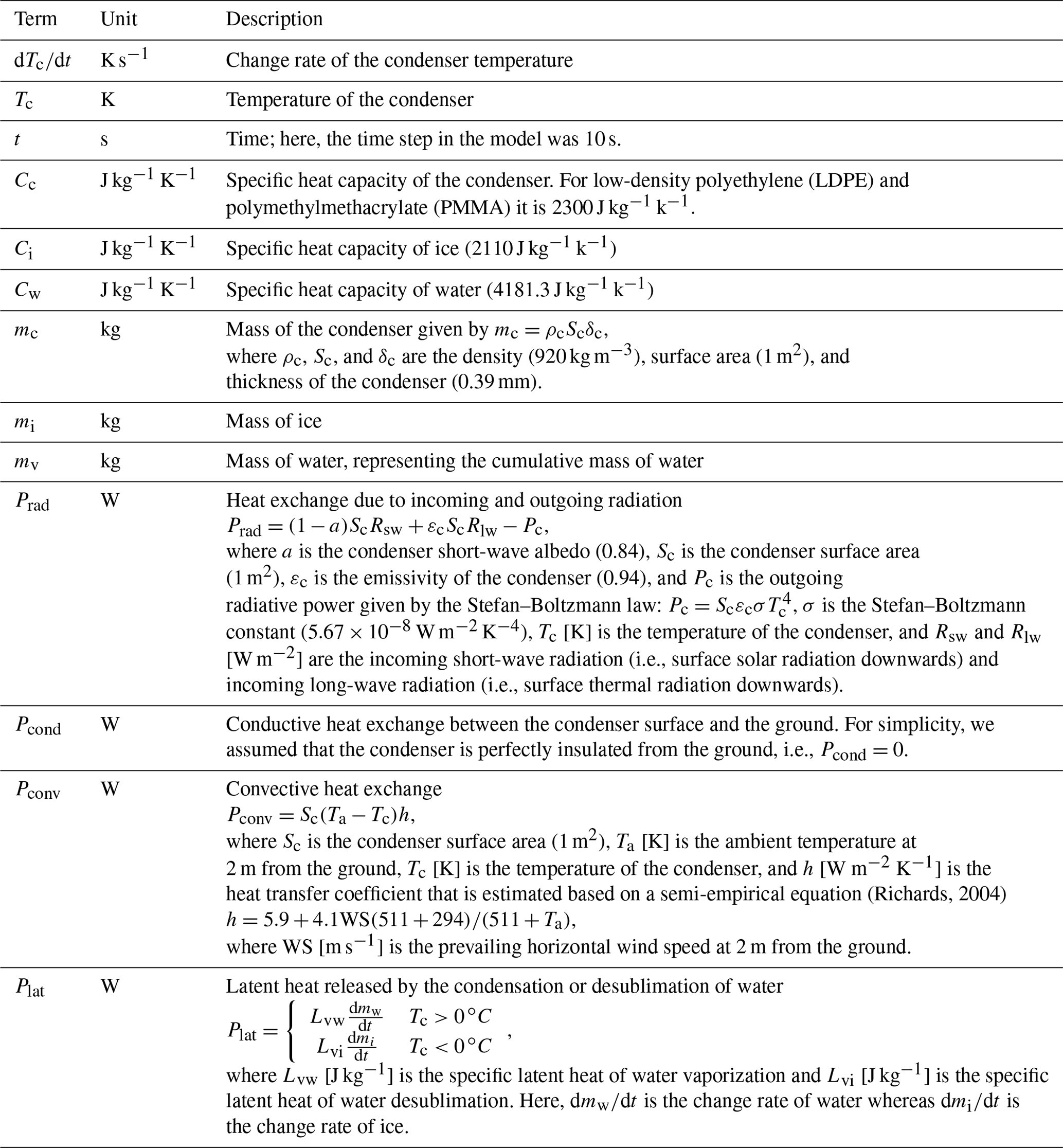
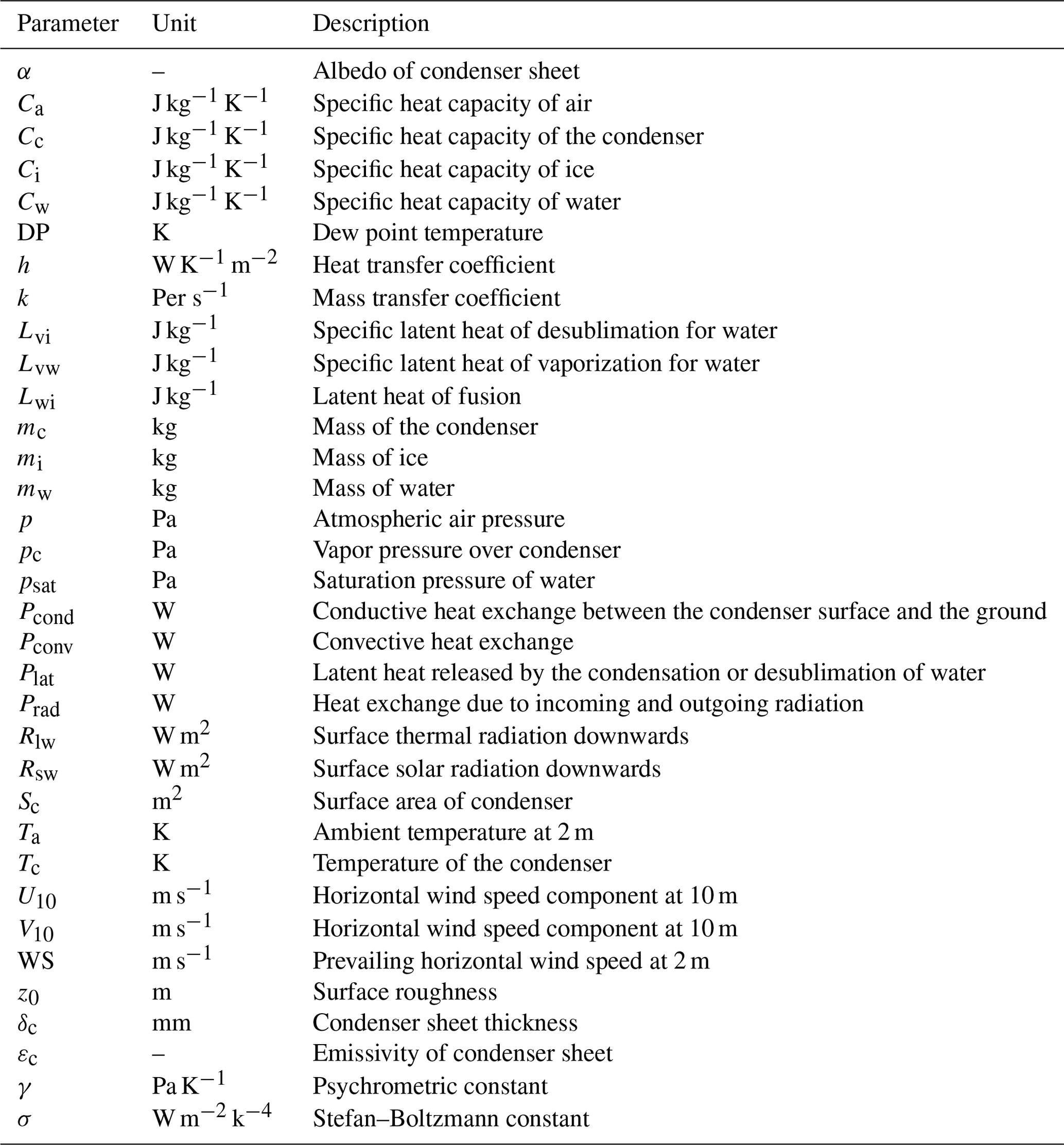
where ddt is the rate of change of the condenser temperature. Cc, Cw, and Ci are the specific heat capacity of the condenser, water, and ice, respectively. Here, mc, mw, and mi are the mass of the condenser, water, and ice, respectively. The righthand side of Eq. (2) describes the heat exchange involved in the process: Prad is the net radiation, Pcond is the conductive heat exchange between the condenser surface and the ground, Pconv is the convective heat exchange, and Plat is the latent heat released by the condensation or desublimation of water.
The model was setup so that it assumes similar conditions for the phase change of pre-existing water or ice on the condenser sheet. For instance, if the water on the condenser is in the liquid phase (i.e., mw>0) and the condenser temperature Tc<0∘, then the sheet is losing energy (i.e., the righthand side of Eq. 2 is negative). In that case, instead of solving Eq. (2), Tc is assumed to be constant and the lost mass from the liquid phase of water is transferred to the cumulated mass of ice; i.e., the water is transformed from liquid phase to solid phase. Consequently, Eq. (2) is replaced by
where Lwi is the latent heat of fusion. If the water on the condenser is in the solid phase (i.e., mi>0) and the condenser temperature Tc>0∘, a similar equation is assumed for the change rate of ice mass (mi).
Note that Eq. (3) is not related to the condensation of water; it only describes the phase change of the already condensed water or ice on the condenser. For the water condensation rate, which is assumed independent of Eq. (3), the mass-balance equation is then assumed as
where m represents either the mass of ice (mi) or water (mw) depending on whether Tc is below or above 0∘. Psat(Td) is the saturation pressure at the dew point temperature and Pc(Tc) is the vapor pressure over the condenser sheet. Here, Sc is the condenser surface area and k is the mass transfer coefficient,
where Lvw is the specific latent heat of water vaporization, γ is the psychrometric constant, Ca is the specific heat capacity of air, and p is the atmospheric air pressure. Here, h is the heat transfer coefficient,
where u and Ta are the prevailing horizontal wind speed and the ambient temperature 2 m above the ground. This parameterization of the heat transfer coefficient is taken from Richards (2004). However, the dew model is designed in such a manner that any functional form can be used for the heat transfer coefficient, thus allowing the sensitivity of the modeled dew amounts to the formulation of the heat transfer coefficient to be assessed (see Sect. 3.3 for such an analysis).
In practice, the wettability of the surface affects the vapor pressure Pc directly above it. In other words, Pc is lower over a wet surface; thus, condensation may take place even if Tc>Td. It is also assumed (in Eq. 4) that there is no evaporation or sublimation during daytime even if Tc>Ta. Furthermore, the model simulation resets the cumulative values for water and ice condensation at noon (local time) and takes the preceding maximum value of mw+mi as the representative daily yield given in millimeters on a 1 m2 condenser sheet (i.e., mm m−2 d−1 equals L m−2 d−1).
This way, the model simulation replicates the daily manual dew water collection of the condensed water around sunrise, i.e., after which Tc is often above the dew point temperature. All terms and nomenclature are described in more detail in Tables 2 and 3.
Table 2Description of the dew formation model by listing the terms in Eq. (1).
It should be noted here that, similarly to many numerical models, this model has some limitations that should be considered when interpreting the results. For instance, both heat and mass coefficients are semi-empirical parameters that depend on wind speed (i.e., here we used the parameterization by Richards (2004), which is valid for u<5 m s−1). In addition, the 10 s time step in the model does not allow condensed water droplets to be eliminated on the condenser surface by evaporation. Moreover, the model predicts any dew condensation regardless of whether it is collectible or not; therefore, it is expected to overestimate dew yield. The spatial data resolution is ∼30 km, which limits the model's ability to resolve local microclimates, particularly in areas with complex topography where the topography can modify the large-scale winds and lead to large variations in local temperatures. However, when considering cumulative dew yield over long time periods the model performs well. Therefore, as the model uses the meteorological gridded dataset (ERA-Interim), which is readily available for the whole globe, it can be applied anywhere in the world including other arid and semi-arid areas even if they lack observations.
2.3 Cluster analysis
Cluster analysis (CA) is an effective statistical tool and technique that groups similar data points such that the points in the same group are more similar to each other than the points in the other groups. The group of similar data points is called a cluster, which can be used for various applications (Corporal-Lodangco and Leslie, 2016; Güngör and Özmen, 2017). There are two main clustering methods: hierarchical and non-hierarchical cluster analysis. Hierarchical clustering (used in this study) combines cases into homogeneous clusters where objects at one level are combined with objects at another level and produce clusters that are not allowed to overlap (Bunkers and Miller, 1996; Yim and Ramdeen, 2015). Two different strategies for hierarchical clustering exist: agglomerative and divisive (Lior and Maimon, 2005). In this study, we used hierarchical agglomerative clustering (HAC, Nielsen, 2016), which starts with N clusters (i.e., here, the total number of grid points) each containing one object and then joins the two objects that are most “similar”. This process continues until only one cluster containing all the data remains (Bunkers and Miller, 1996). In order to decide which clusters should be combined (for agglomerative), a measure of dissimilarity between sets of observations is required. The similarity measurement is a critical step in hierarchical clustering as it can influence the shape of the clusters (Nielsen, 2016). With metric data, the most commonly used distance measure (a measure of the distance between pairs of observations) is “Euclidean distance”. The Euclidean distance (dij) between two objects i and j in a two-dimensional data matrix is simply the squared difference between two observations for each of the p variables summed over the variables and k is the number of observations (Fovell and Fovell, 1993; Dokmanic et al., 2015). This can be written as
Here we applied this method to a two-dimensional matrix (2496×14 610), where the number of rows represented the number of spatial grid points in the model simulation domain and the number of columns represented the time (i.e., cumulative daily dew yield).
After all distances were calculated, the next step is to merge the two closest entries to form a new cluster based on a linkage criterion. The linkage criterion determines the distance between sets of observations (here, the spatial grid points) as a function of the pairwise distances between observations. There are some commonly used linkage criteria: single linkage, complete linkage, average distance, and Ward's minimum variance methods, which differ in the way distances between entries are calculated and how the two closest entries are defined (Stooksbury and Michaels, 1991; Murtagh and Legendre, 2014). In this study, Ward's minimum variance method (Ward, 1963) is used. This method is the most frequently clustering technique used in climate research (Yokoi et al., 2011; Mimmack et al., 2001; Siraj-Ud-Doulah and Islam, 2019) and gives the most consistent clusters (Kalkstein et al., 1987). It calculates the means of all variables (the amount of dew) within each cluster, then calculates the Euclidean distance to the cluster mean of each case, and finally sums across all grid points (Unal et al., 2003).
In any CA, the optimal number of clusters is an important issue. There is no reliable and universally accepted method to determine the optimal number of clusters. Kaufmann and Weber (1996) (see also Unal et al., 2003 and Burlando, 2009) suggested showing the total variance of subsequent merged clusters as a function of the number of remaining clusters. This information can be used as an indicator to decide the number of clusters, but a visual check of the result can still help to make the right decision. The suitable number of clusters has to be chosen somewhere in the transition between the distance values when a sudden decrease is observed as illustrated in Fig. 2a. In our case, few steps at N=3, 4, 6, 7, and 10 are recommended as optimal numbers of clusters. By visualizing all these steps, N=6 was found to be the best number of clusters for this study because fewer clusters (i.e., 3 and 4 clusters) were not able to capture the different climate and dew zones. Furthermore, choosing more clusters (i.e., 7 and 10 clusters) gives some groups that replicate each other. The results of hierarchical clustering are usually presented in a dendrogram (Nielsen, 2016). The dendrogram of our 6 clusters is shown in Fig. 2b.
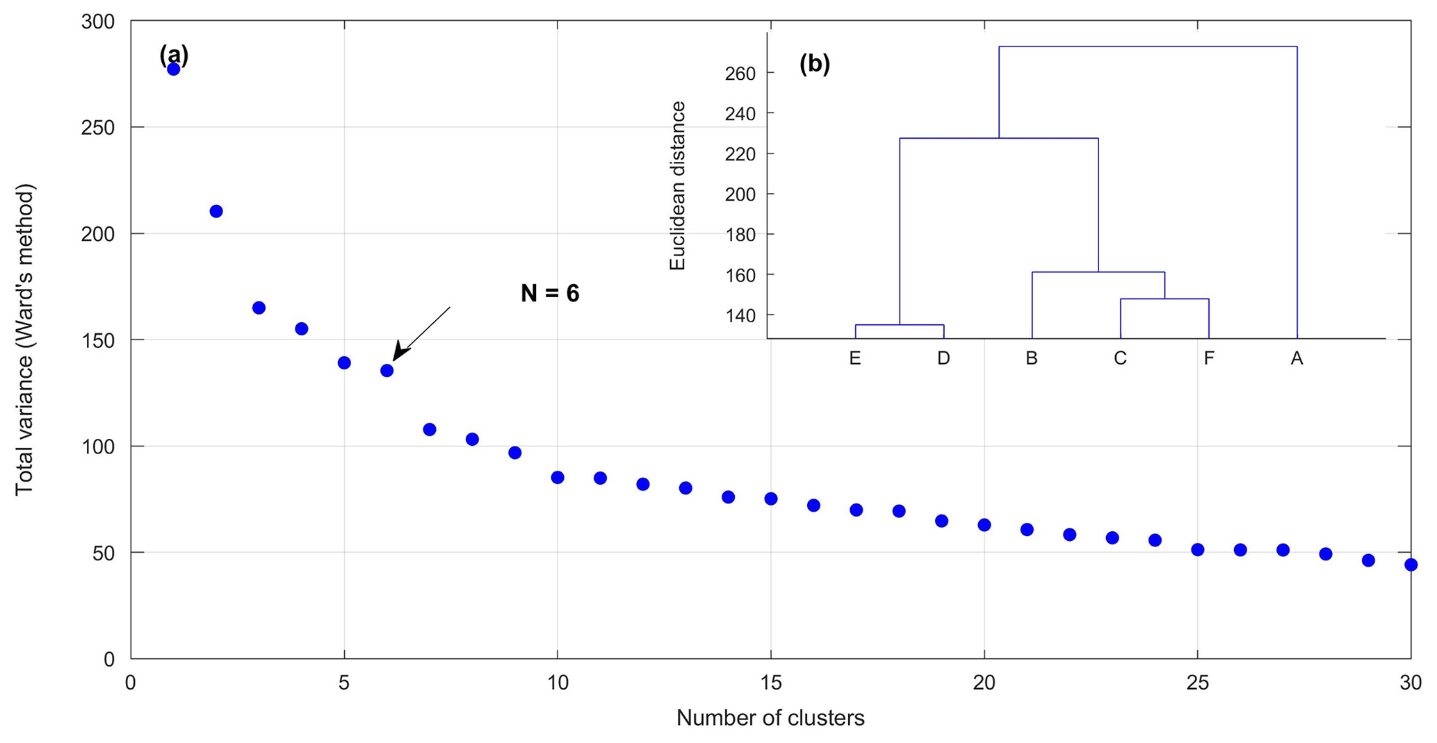
Figure 2(a) Distance level at which two clusters are merged as a function of the number of clusters that result when the Ward linkage method is applied to daily dew yield data from 1979–2018. N is the optimal number of clusters that has been chosen for this study. (b) Dendrogram of 6 clusters.
3.1 Spatial–temporal variation of dew occurrence and yield
According to the model simulation results (cumulative daily dew yield in the form of dew and hoarfrost), dew formation occurred almost everywhere in Iran, as illustrated in Fig. 3, which shows the seasonal occurrence of dew as a fraction of days with any dew yield. The frequency of dew occurrence was more than 80 % (∼75 d) in most areas of Iran in wintertime (December–February; Fig. 3a). The mean occurrence of dew was rather similar during spring (March–May, ∼50 d; Fig. 4b) and autumn (September–November, ∼40 d; Fig. 3d) with the highest number of dew days – more than 90 % (∼80 d) – in the mountainous and coastal areas and the lowest – less than 40 % (∼35 d) – mostly in the dry interior and eastern areas. The lowest frequency of dew occurrence (i.e., less than 10 d) was in summer (June–August, Fig. 3c) when dew formation was limited to a narrow part along the Caspian Sea and the northern domains of the Alborz Mountains.
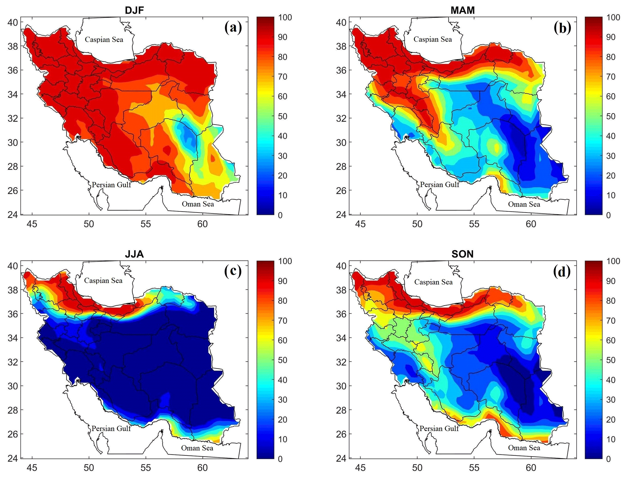
Figure 3Frequency of dew occurrence as a fraction of the days presented as an overall seasonal mean during 1979–2018. (a) Winter (December, January, and February), (b) spring (March, April, and May), (c) summer (June, July, and August), and (d) autumn (September, October, and November).
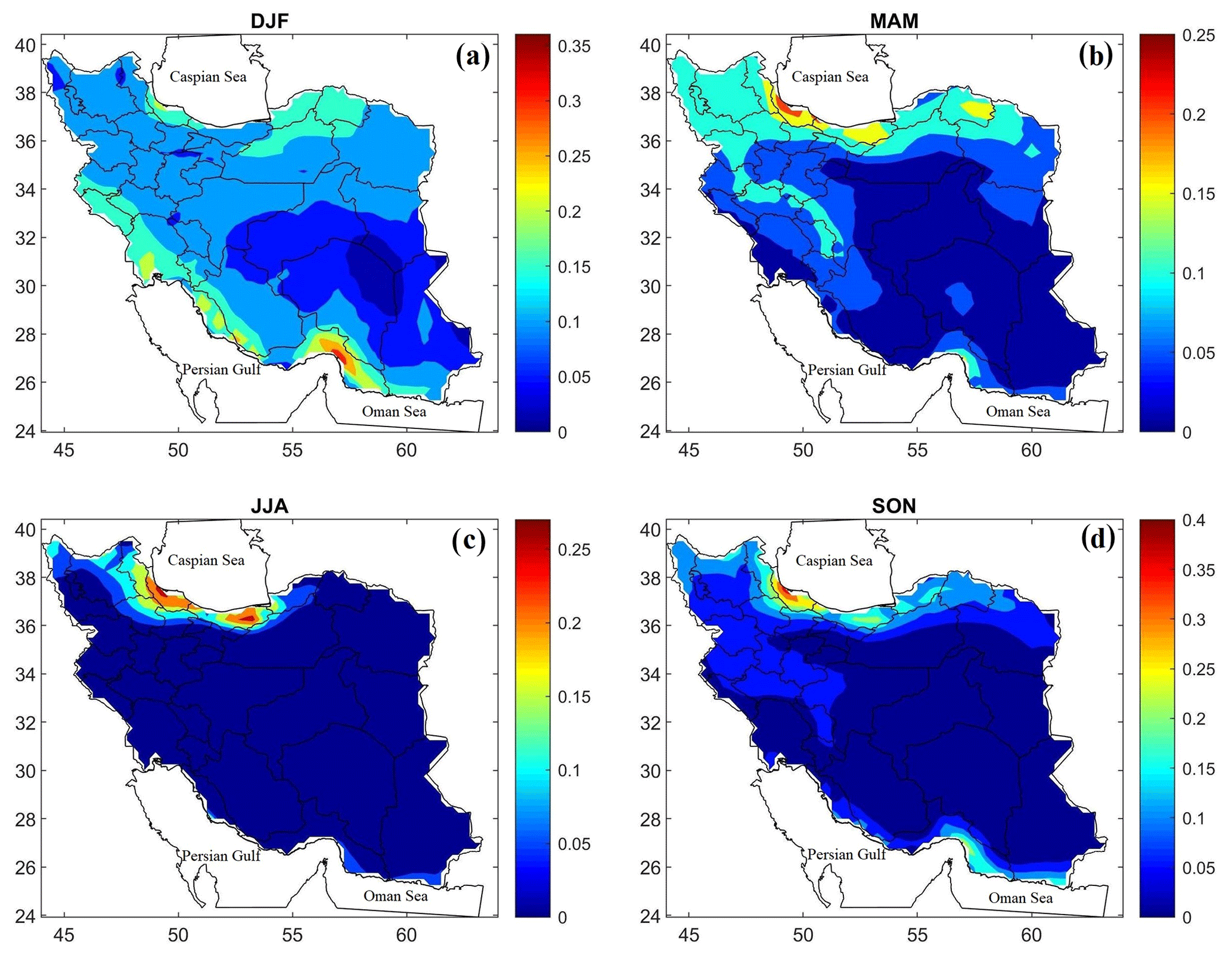
Figure 4Cumulative dew yield [L m−2 d−1] presented as an overall seasonal mean during 1979–2018. (a) Winter (December, January, and February), (b) spring (March, April, and May), (c) summer (June, July, and August), and (d) autumn (September, October, and November).
Limiting the dew occurrence analysis to days with dew yield > 0.1 L m−2 d−1 also confirmed the seasonal characteristics of the temporal–spatial occurrence of dew. However, in this case, the frequency of dew occurrence days was less (in the range of 6–45 d for summer and winter, respectively; Fig. S1 in the Supplement) and the spatial scale of dew formation shrank to include only a few parts of the coastal and high mountain regions during spring, summer, and autumn. This notable difference between the two maps (i.e., Figs. 3 and S1) is associated with the model setup. The model tends to forecast any dew event, regardless of whether it can be collectible or not. In practice, very small dew quantities are generally not harvestable as droplets remain pinned to the condenser surface and gravity cannot lead them to the collection tank.
We subsequently calculated the seasonal daily means of the cumulative dew yield (Fig. 4), which show a clear seasonal cycle with high dew yields during the winter and low yields during the summer in most parts of Iran. The monthly means of the cumulative dew yield are shown in Fig. S2. Both seasonal and monthly maps show that the mountain regions had dew occurrence throughout the year with mean cumulative daily dew in the range of 0.11–0.18 L m−2 d−1. In winter, dew occurred almost everywhere in Iran with the highest yields in the southern part of the Persian Gulf and Oman Sea coastline (mean cumulative daily dew in the range 0.15–0.23 L m−2 d−1). In spring (i.e., April and May), a spatial pattern was observed that indicated the formation of dew was mainly parallel to the mountain range – Alborz (East–West) and Zagros (northwest and southeast). The reason could be related to the temperature, which increases, and relative humidity, which decreases, during these spring months. Therefore in spring in most areas, conditions for dew formation were not present except in high elevation areas where the conditions still favor dew formation. During summer and until the middle of autumn (i.e., July–October), a unique spatial pattern was evident that shows the distribution of dew formation was limited to a narrow belt in coastal areas in the north along the Caspian Sea. In all other areas, the monthly amount of dew yield was almost zero.
3.2 Cluster analyses – dew formation zones
3.2.1 Dew zones – a general overview
According to our cluster analysis (CA) summarized in Sect. 2.2, we identified six dew formation zones in Iran (Fig. 5). The amount of daily dew yield in Iran and the related climatological parameters (e.g., temperature and relative humidity) for dew formation as well as the percentiles (i.e., 25 %, median, 75 % and 99 %) of daily dew yields as averages for each cluster are listed in Table 4. As will be shown in this section, the dew formation zones in Iran are clearly aligned with topography, sources of moisture, and climate zones. Furthermore, the mountains and seas played major roles in the spatial distribution of dew formation zones. Note that the maximum daily dew yield in this section is presented as the 99th percentile of daily dew. In order to gain insight into the climatological condition in each dew zone, we selected one synoptic station in each dew zone and investigated some related meteorological parameters (e.g., temperature, humidity, and wind speed) in the nighttime hours (i.e., 18:00, 21:00, 00:00, 03:00 LT), when dew formation occurs, for the time period 1980–2010 (30 years), which is shown in Figs. 7 and 8.
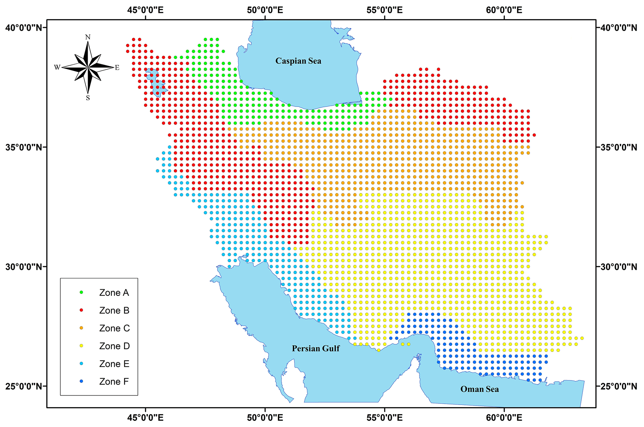
Figure 5Dew formation zones based on the cluster analysis of the daily cumulative dew yield during 1979–2018.
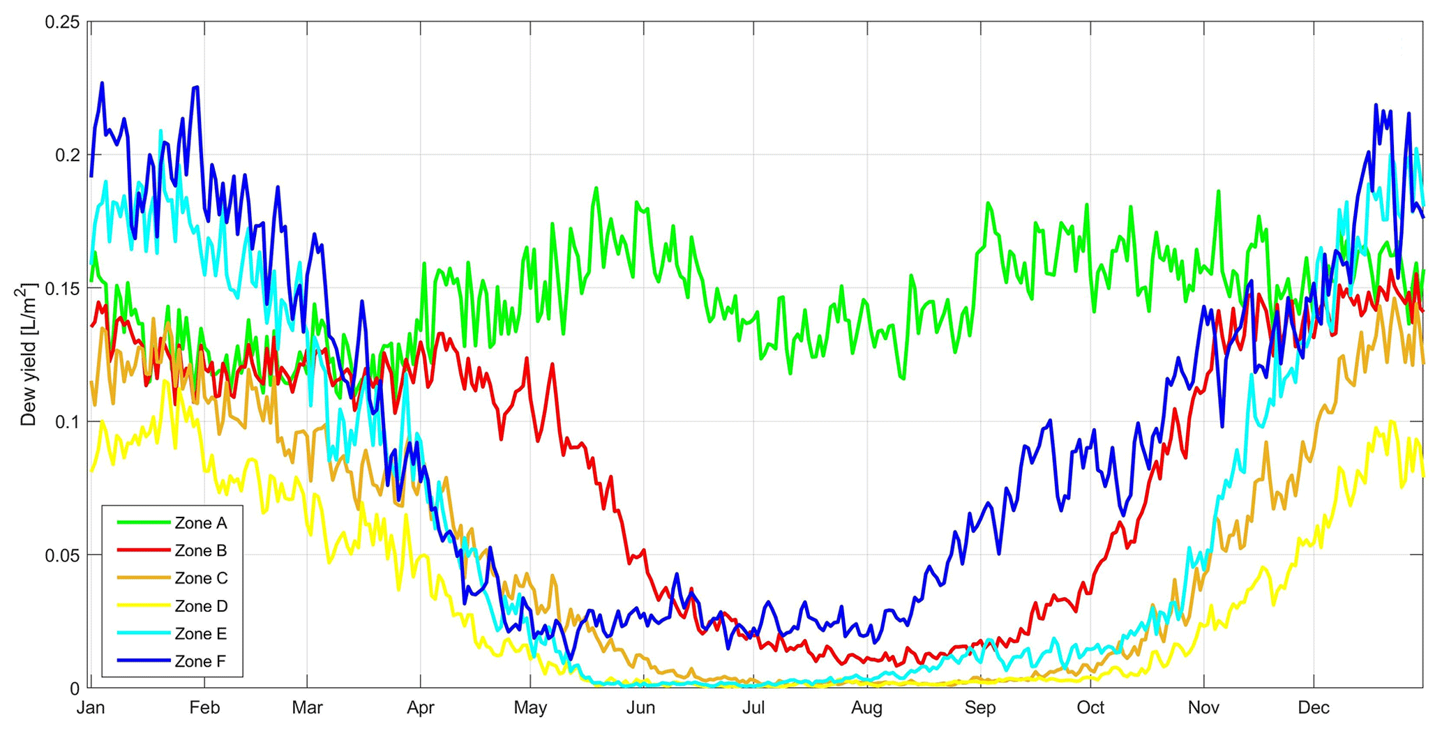
Figure 6Long-term mean seasonal variation of the cumulative daily dew yield. Note that color coding on this figure is the same and corresponds to the dew formation zones in Fig. 5: dew zone A (Caspian Sea; green), Zone B (Zagros region; red), Zone C (Central Iran; orange), Zone D (Lut Desert; yellow), Persian Gulf zone (light blue), and Oman Sea zone (dark blue). The percentiles (i.e., 25 %, median, 75 % and 99 %) of the daily dew yields as averages for each cluster are presented in Table 4.
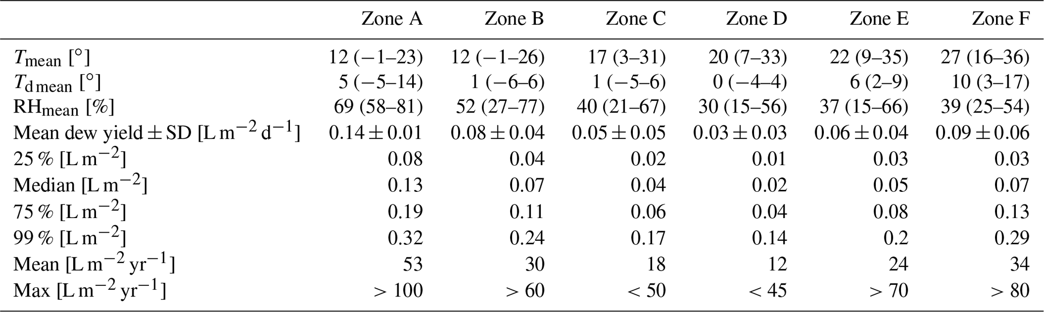
Table 4Dew formation zones and their climate features (i.e., mean (min–max) values for meteorological parameters (T, Td, RH)) as well as statistical analysis for overall mean daily cumulative dew yield (i.e., SD, 25, 50, 75th and 99th percentile as daily max as well as yearly max dew yield).
Dew zone A – Caspian Sea region
We identified the first dew formation zone as the “Caspian Sea region”, which covered the southern shores of the Caspian Sea and the northern domains of the Alborz Mountains. This dew zone includes about 7 % of the total land area of Iran (Fig. 5), which also includes the largest forest area in Iran. The overall mean daily dew yield in this region was ∼0.14 L m−2, which was the highest among all of the dew zones, and the maximum dew yield was 0.30 L m−2 d−1 (Table 4). Interestingly, this dew zone is different compared to the other dew zones concerning the annual cycle of dew formation; in this dew zone, dew formation occurred throughout the year whereas all other zones exhibit a strong annual cycle (Fig. 6). The mean frequency of dew occurrence in this zone was more than 330 d yr−1. Even in summer, when dew almost vanished in other dew zones, this zone had a significant amount of dew yield (Fig. 4). The mean yearly dew yield in this region is estimated at about 53 L m−2 and the maximum yield is more than 100 L m−2. The high potential of dew formation in this zone during the year is due to very suitable climatological and geographical conditions. The synoptic station Ramsar located in this dew zone shows the climate of dew zone A to be characterized by low temperature, high humidity, and the smallest dew point depression (i.e., the smallest difference between the temperature and dew point) along with little variation in the relative humidity and dew point depression throughout the year (Fig. 7a). Moreover, due to being a forest area, the wind speed is relatively low (Fig. 8a), which favors dew condensation.
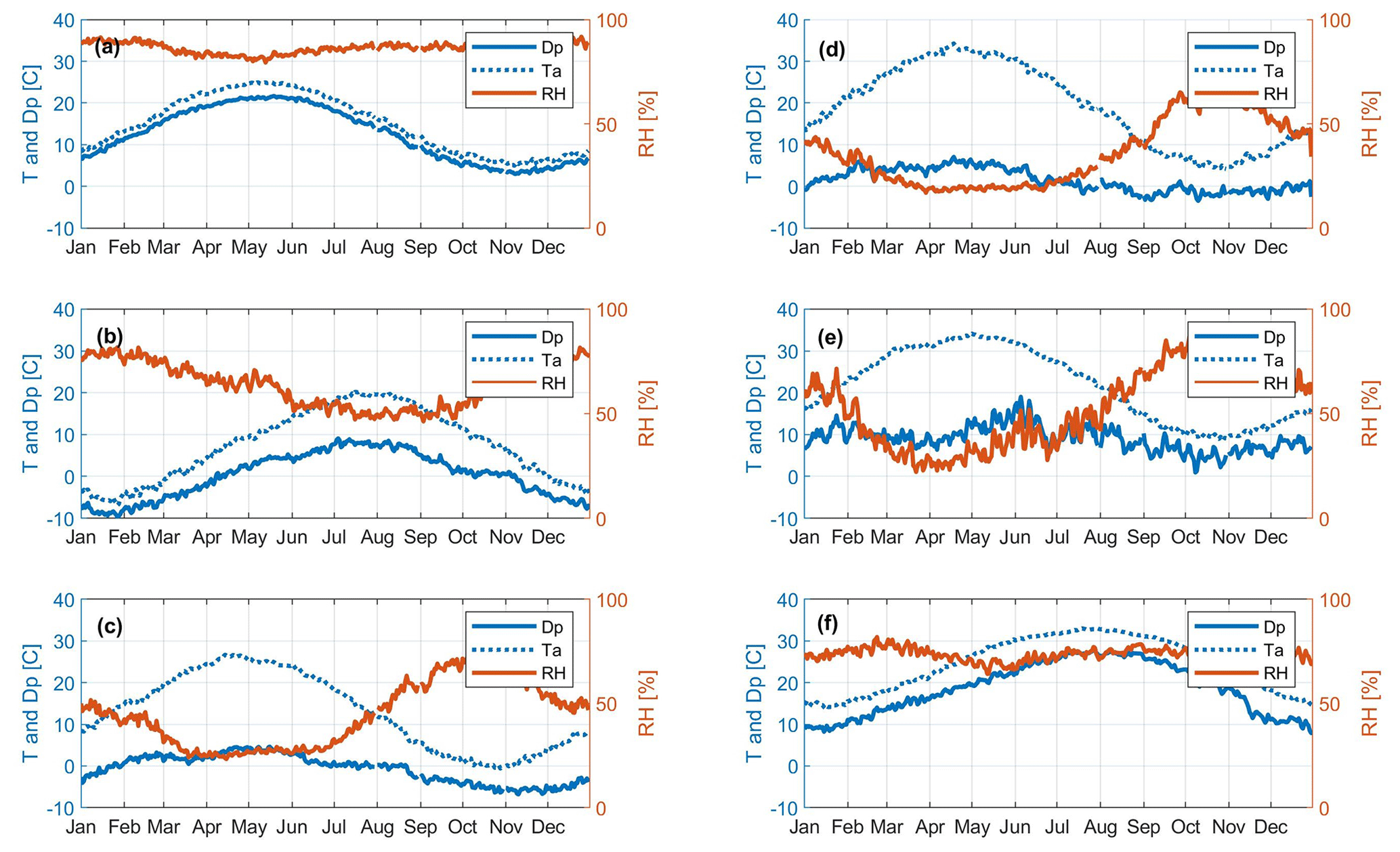
Figure 7Nighttime (i.e., 18:00, 21:00, 00:00, 03:00 LT) long-term mean (1980–2010; 30 years) of dew point temperature (Dp) temperature (Ta), and relative humidity in six selected stations located in dew zone A–F. (a) Ramsar (dew zone A); (b) Zanjan (dew zone B); (c) Isfahan (dew zone C); (d) Tabas (dew zone D); (e) Ahvaz (dew zone E), and (f) Bandar Abbas (dew zone F). Data were obtained from the meteorological organization of Iran.

Figure 8Nighttime (i.e., 18:00, 21:00, 00:00, 03:00 LT) long-term mean (1980–2010; 30 years) of wind speed in six selected stations that are located in dew zone A–F. (a) Ramsar (dew zone A), (b) Zanjan (dew zone B), (c) Isfahan (dew zone C), (d) Tabas (dew zone D), (e) Ahvaz (dew zone E), and (f) Bandar Abbas (dew zone F). Data were obtained from the meteorological organization of Iran.
Dew zone B – Zagros Mountains
Dew zone B included the Zagros Mountains (i.e., the northern and central parts) and the eastern part of the Alborz Mountains. This dew zone covered about 15 % of Iran (Fig. 5) and represented a mountain climate with very cold and dry weather in winter and mild weather in summer (Fig. 7b; Zanjan station). Furthermore, due to the high elevation, the diurnal variation of temperature within this dew zone is large. These areas receive high levels of solar radiation during the daytime and reflect it back quickly to space in the form of long-wave radiation during nighttime. Therefore, the temperature drops rapidly during nighttime. Enough moisture in the atmosphere, in addition to this strong nocturnal cooling, favored dew formation. The overall mean daily dew yield and variation in this region was 0.08±0.05 L m−2 d−1 and the highest dew yield was 0.23 L on a 1 m2 condenser sheet. The highest amount of dew yield in this dew zone was observed during spring when the prevailing winds in this region are typically westerlies and accompanied by moderate to high relative humidity (Fig. 7b) and low wind speed (Fig. 8b). The amount of dew yield decreased rapidly after May and was almost absent during summertime (Fig. 6). This is a result of higher temperature (i.e., due to atmosphere transparency and receiving high solar radiation) and lower relative humidity (Fig. 7b) and also the lack of efficient moisture sources in this dew zone. In general, the mean frequency of dew occurrence in this zone was 63 % (∼245 d). The mean yearly dew yield in this zone was about 30 L m−2 and the maximum was more than 70 L m−2 (Table 4).
Dew zone C – Central Iran
The third dew zone is the Central Iran region. Central Iran consists of the southern slopes of the Alborz Mountains in the north, the Zagros Mountains in the south, and the central Iranian ranges. These areas are mostly hot and very dry. The Alborz and Zagros mountains prevent moisture penetration from the Caspian Sea and westerlies so that the amount of water vapor pressure is very low (∼7 hPa; Masoudian, 2011). This zone covered about 20 % of Iran and included the Kavir Desert basin, Salt Lake, and some parts in the northeast (Fig. 5). The overall mean daily dew yield in this region is estimated to be about 0.05 L m−2 and the maximum yield (99th percentile) was about 0.21 L m−2 d−1. The average yearly dew yield in this region was about 18 L m−2 and the maximum yield was less than 50 L m−2 yr−1. The dew period in this zone starts in autumn and continues until mid-spring (i.e., October–April); however, the frequency of dew occurrence (>0.1 L m−2 d−1) is about 80 d. Isfahan station is located in this dew zone and is representative of the climate of this dew zone. The dew point temperatures are very low (mainly around or less than zero) all year round and have slight annual variation (Fig. 7c). The relative humidity is low in spring but increases in Autumn (Fig. 7c) when temperatures start to decrease and dew formation also starts. Furthermore, the wind speed is quite weak (less than 2.5 m s−1 on average, Fig. 8c) and does not have a pronounced annual cycle. Therefore, humidity and temperature are most likely the key factor in formation of dew in this station. More specifically, once relative humidity starts increasing and temperature decreases (in autumn and winter), dew can also form.
Dew zone D – Lut Desert
We identified the fourth dew zone (i.e., Dew zone D) that included the Lut Desert (175 000 km2; Alizadeh-choobari et al., 2014), which is an arid and hyper-arid desert (Fig. 5). This zone, with 35 % of all grid points in the land areas of Iran, is the largest dew zone; however, it has the least dew occurrence (∼15 d yr−1 with dew yield > 0.1 L m−2 d−1) and a mean yield of 0.03 L m−2 d−1. Indeed, this part of the country includes the driest areas (i.e., water vapor pressure is <5 hPa). Based on a survey conducted by scientists at NASA's Earth Observatory during the summer of 2003–2009 (see Temperature of Earth: https://www.universetoday.com/14367/planet-earth, last access: 7 August 2021), the Lut Desert was the hottest (∼71∘) land surface on Earth (see also Khandan et al. (2018)). The synoptic station Tabas is located in this dew zone and has a climate characterized by high temperatures (higher than the synoptic stations we considered in dew zones A, B, and C) and low relative humidity in summer (Fig. 7d). In addition to the dryness, these areas have high diurnal variations in temperature, mostly a clear sky, extremely sparse vegetation, and frequent high wind speed. In wintertime, the temperature decreases and the moisture increases (Fig. 7d) as a result of the westerly prevailing wind; thus, this dew zone experienced its highest amount of dew yield in winter. In contrast, in the warm season (i.e., May–September) dew was almost completely absent (Fig. 6). The reason is due to high temperature, longer daytime duration, and a strong north–south pressure gradient between the thermal low-pressure system over the desert lands and a cold high-pressure over the Hindu Kush in northern Afghanistan (Alizadeh-choobari et al., 2014) that generates the strong summer wind called “the Sistan wind of 120 d”. It has this name because it occurs during late May through late September (about 4 months) in the east and southeast of the Iranian Plateau, particularly the Sistan Basin. The typical wind speed of the Sistan is 30–40 km h−1, but it could occasionally exceed 100–110 km h−1, which impedes dew formation during the summer season. Thus, the key factors for dew condensation (high humidity and low wind speeds) are not present for most of the year in this dew zone. Consequently, the average yearly dew yield in this zone was low – about 12 L m−2 – and the maximum yield was about 40 L m−2 yr−1.
Dew zone E – Persian Gulf region
The Persian Gulf dew zone included the coastal line of the Persian Gulf and some parts of the western half of the land areas in Iran (∼9 % of all grid points; Fig. 5). The overall mean daily dew yield is about 0.06 L m−2, which is lower than the other coastal zones in the north (i.e., Caspian Sea; dew zone A) and south of Iran (i.e., Oman Sea; dew zone F). However, the maximum daily dew yield in winter (i.e., December–February) was higher than that in the Caspian Sea zone. Indeed, this dew zone benefits from two huge sources of moisture (i.e., the Persian Gulf and Karun river), although high temperatures (e.g., as observed at the synoptic station Ahvaz; Fig. 7e), thermal high pressure, and dry winds, especially during the warm season (i.e., May–September), do not favor the formation of dew. Therefore, the period of dew formation was about 7 months starting in October and ending in April. However, the frequency of dew occurrence > 0.1 L m−2 d−1 is about 117 d during November–February (Fig. 6) when relative humidity is at its highest level and temperature and wind speed are relatively low compare to the rest of the year (Figs. 7e and 8e). The average yearly dew yield in this zone was about 24 L m−2 and the maximum was >70 L m−2 yr−1 (Table 4).

Figure 9Mann–Kendall trend test on mean yearly dew yield over the years 1979–2018 as predicted by Sen's slope estimator. Only locations with a statistically significant trend (p<0.05) are shown. Red points present locations with a negative trend regardless of their decreased values, and the white parts did not show any significant trend at (p<0.05).
Dew zone F – Oman Sea region
The coastline along the Oman Sea and the Strait of Hormuz formed the sixth dew zone, which is also the smallest dew zone in Iran covering only 5 % of the grid points (Fig. 5). The overall mean daily dew yield in this zone was about 0.09 L m−2 and the maximum dew yield was about 0.23 L m−2 d−1 (Table 4), which was the highest among all dew zones. This is not surprising because this region benefits from a generous source of moisture (i.e., the Oman Sea, Persian Gulf, Arabian Sea, and Indian Ocean through the summer monsoon). Observations from the station Bandar Abbas confirm the presence of a moisture source, as the difference between the temperature and dew point temperature is quite small (about 5∘) and constant throughout the year. However, despite these conditions, the formation of dew was mostly limited to the cold season (i.e., starting in September and ending by March; Fig. 6); during the warm season (i.e., April–August), dew occurrence was rare (Fig. 6). The reason is likely due to the increase in wind speed (as shown by observations at the synoptic station Bandar Abbas; Fig. 8e) and the temperature during summer. In particular, in the warm season, high temperatures lead to the formation of low-pressure systems (i.e., the Gang low pressure system and Persian Gulf low pressure system) over the seas, which intensified the hot and humid conditions in the southern coastal region. High humidity results in amplified long-wave radiation downwards and therefore less radiative cooling. In addition, due to the strong gradient between the low pressure over the Persian Gulf and the high pressure over Saudi Arabia, an intense airflow is stimulated such that condensation does not occur despite high humidity. Lastly, although this zone had the highest daily dew yield, it does not have the highest yearly yield (i.e., >80 L m−2) since the frequency of dewy days (∼150 d) in this zone is lower than in dew zone A (the Caspian Sea region; Fig. 7).
Table 5Correlation between long-term mean daily dew yield and meteorological parameters obtained from ERA-Interim for the time period 1979–2018 and Sen's trend slope in the meteorological variables per decade (i.e., 10 years).
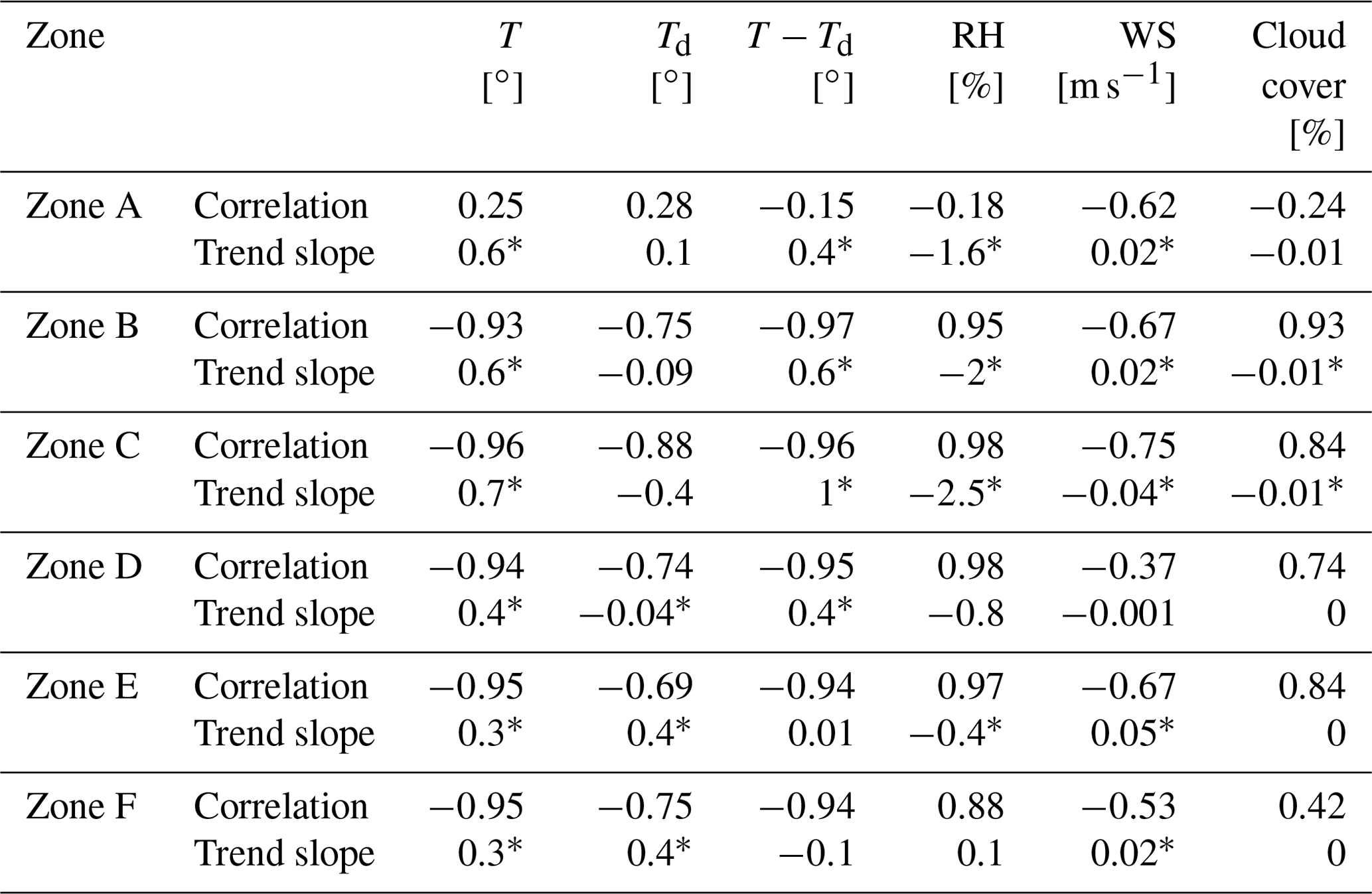
* Values with an asterisk indicate a statistically significant trend (p<0.05).
3.2.2 Long-term temporal variation in dew formation zones
In order to investigate the long-term (1979–2018) variation of dew formation, we applied the Mann–Kendall trend test (Pohlert, 2016) to the yearly means of dew yield with a confidence level of 95 %. Figure 9 shows the statistical significance (p<0.05) of the overall changes in the mean yearly dew yield. The result of this trend analysis showed that in more than 60 % of the land areas in Iran (i.e., mostly dew zones C and F and the northern half of dew zones B and D), dew formation has decreased during the past 40 years. The remaining parts of Iran did not show any significant trend (α=5 %); however, their negative slope (82 % of the remained grid points) might be a sign of a future decrease in dew formation for these regions. Such negative trends in dew yield over a wide geographical region could be due to different reasons that control the condensation process. To identify potential causes for the detected decrease in dew formation, we first calculate correlations between the dew formation and meteorological parameters (temperature, dew point temperature, dew point depression, relative humidity, wind speed, and cloud cover obtained from ERA-Interim) for each dew formation zone (Table 5). Subsequently, we calculate the trend for each of the six meteorological variables.
The correlation analysis (i.e., Pearson's correlation) revealed that dew formation in almost all dew zones (i.e., B–F) has a very strong negative correlation (values of −0.93 to −0.95) with temperature, a strong positive correlation with relative humidity (values of 0.88 to 0.98), and a negative correlation with the dew point depression (−0.69 to −0.88). In contrast, dew zone A (the Caspian Sea) has weak correlations between dew formation and temperature, relative humidity, and dew point temperature indicating dew formation in this region is controlled by different processes. In addition, zone A is the only zone to have a weak and negative correlation between dew formation and cloud cover. These huge differences between dew zone A and other zones are likely due to differences in topography as dew zone A is mainly covered by forests and the behavior of some climatological variables can be different than the rest of the areas. A moderate negative correlation between dew formation and wind speed (−0.62) does exist in zone A, which may indicate that wind speed is the meteorological parameter with the most influence on dew formation in Zone A.
When the long-term trends are considered, air temperature, which has a negative effect on dew formation, showed a significant positive trend (p<0.05) in all dew zones over the 40 years. The magnitude of these changes for zones A–F was 0.6, 0.6, 0.7, 0.4, 0.3, and 0.3∘ per decade, respectively. Relative humidity (RH) and cloudiness had a positive effect on dew formation (except in Zone A); however, they both had a negative trend over 40 years. The average decrease in relative humidity for the dew zones (i.e., A–E) was about 1.5 % per decade (Table 5). Therefore, the increase in temperature and decrease in RH and cloudiness can largely explain the decreasing trend in dew yield during the last 4 decades (1979–2018).
3.3 Uncertainties in the dew model simulation results
A detailed investigation of the model setup, i.e., input parameters (e.g., emissivity and albedo), wind profile assumptions, and heat transfer assumptions, revealed that the dew yield estimation is very sensitive to the heat transfer coefficient. In order to obtain an estimation of the final uncertainties in the model simulation results (i.e., daily dew yield) caused by the heat transfer coefficient, we ran the model with eight different parameterizations of the heat transfer coefficients for four grid points (Table 6) for one year (2000). We selected four stations or grid points (red stars in Fig. 1) in different dew zones: Ramsar station in dew zone A, Zanjan in dew zone B, Tabas in dew zone D, and Bandar Abbas in dew zone F.
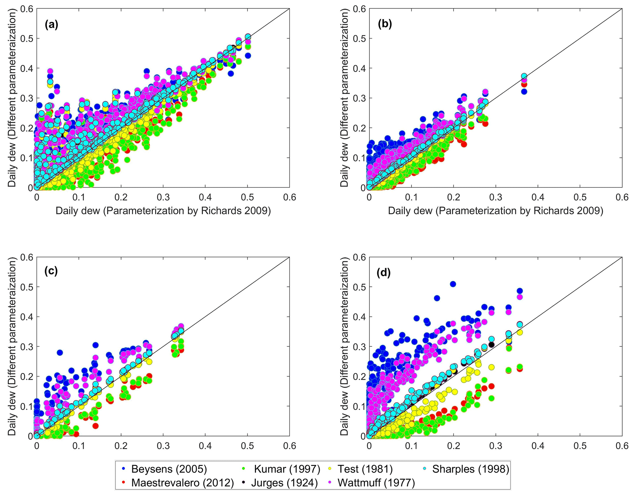
Figure 10Scatter plots of the daily dew yield obtained from parameterization by Richards (2004) against seven different parameterizations listed in Table 6 for four stations in different areas of Iran. (a) Ramsar (forest and coastal area in the north), (b) Zanjan (mountainous area), (c) Tabas (desert area in central Iran), and (d) Bandar Abbas (arid coastal area in the south). The black lines are the 1:1 relationship.
Table 6A selection of eight parameterizations for the heat transfer coefficient, the mean±std daily dew yield, and the mean differences between daily cumulative (L m−2 d−1; negative values indicate the underestimated dew yield relative to the Richard's parameterization and positive values indicate the overestimated dew yield) dew yield caused by each parameterization in four selected stations compared to the coefficient used in this study (i.e., Richards, 2004). The first three are studies on dew formation. Here, u and Ta are the horizontal wind speed and air temperature at 2 m height and L is the characteristic length of the condenser (e.g., 1 m).

Figure 10 shows the daily dew yields estimated using the parameterization by Richards (2004, this study) against the daily dew yields obtained from the seven other parameterizations listed in Table 6. For all four grid points considered, the parameterizations of Beysens et al. (2005) and Watmuff et al. (1997) give the largest estimates of daily dew yields whereas the parameterizations of Kumar et al. (1997) and Maestre-Valero et al. (2011) give the lowest estimates (Fig. 10, Table 6). Figure 10 also demonstrates that the largest differences occur for the very low values of daily dew yield.
The absolute differences in daily dew yields between the parameterizations are calculated in Table 6. At Ramsar (located in dew zone A in a forested region), the daily mean dew estimates range from 0.10 to 0.19 L m−2, which is the largest absolute range of four stations. However, the daily dew yield at Ramsar from all parameterizations is the largest of all four stations (Table 6); thus, this station has the smallest relative difference: the smallest estimate of 0.10 L m−2 is 83 % of the value obtained from the Richardson parameterization and the largest estimate of 0.19 L m−2 is 158 %. Bandar Abbas (located in dew zone F, coastal region) also has a large range of daily dew estimates (0.01 to 0.14 L m−2) but combined with the much lower daily dew yield (0.04 L m−2 from the Richards parameterization) means this grid point has a much larger relative variation (25 % to 350 %) in estimated daily dew yields in comparison to Ramsar. The heat capacity parameterization has a strong impact on the modeled daily dew yields; however, the standard deviations of the daily means are also large (Table 6). However, we conclude that the parameterization used in this study – the Richards (2004) formulation – gives estimates that are similar to the average of all methods and are neither much lower nor much higher than the majority of other parameterizations.
In an ideal situation we would compare our model results to observations; however, unfortunately observational data of dew formation in Iran is not available. Therefore, the accuracy of the modeled dew yields in comparison to observational data cannot be performed for this study. However, Vuollekoski et al. (2015, Sect. 2.3 and Fig. 2) and Atashi et al. (2021) presented detailed comparisons between the results from this dew model and observations in other locations where experimental dew data were available. The results of these studies revealed that in most cases the model overestimates the dew yield due to some of the limitations discussed in Sect. 2.2; however, the cumulative sum of observed and simulated dew yield was found to agree well after smoothing down the daily variations.
Iran is a country located in arid and semi-arid regions that has a growing population and has suffered from water scarcity over the last decades. Therefore, finding renewable sources of water is rapidly becoming a necessity. Dew is one of the atmospheric sources of water that can be vital especially in more dry conditions.
The average daily dew yield in Iran was in the range of 0.03–0.14 L m−2 and the maximum was in the range of 0.29–0.52 L m−2 d−1. Our model-based results are largely in agreement with previous observational dew measurement studies conducted in similar climates (i.e., arid and semi-arid, coastal desert, Mediterranean) using planer dew condensers. However, the quantitative estimates of dew formation can differ between stations located within the same climatic zone. For instance, the reported values for average and maximum daily dew yield for a semi-arid Mediterranean climate (similar to dew zone A and some parts of zone B in Iran) was 0.04 and 0.33 L m−2 in Zadar (France; Muselli et al., 2009), 0.09 and 0.48 L m−2 in Komiză (Croatia; Muselli et al., 2009), 0.04 and 0.27 L m−2 in Beirut (Lebanon; Tomaszkiewicz et al., 2015), 0.06–0.19 and 0.48 L m−2 in a semi-arid coastal area in southwestern Madagascar (Hanisch et al., 2015), and 0.13 and 0.46 L m−2 in Beiteddine village (Lebanon; Tomaszkiewicz et al., 2017). The coastal desert area (i.e., Zone E and F) can be compared with the observed values in Nitzana, Israel (mean: 0.09 L m−2; Kidron, 1999); Dhahan, Saudi Arabia (mean: 0.22 L m−2 d−1; Gandhisan and Abualhamayel, 2005); and Panandhro, India (mean: 0.18 and max: 0.56 L m−2 d−1; Sharan et al., 2011). The average frequency of dew occurrence in Iran was 102 d, while the average number of rainy days in Iran is 38 d (Kashki and Dadashi Rudbari, 2017), suggesting that dew is more frequent than rain. Furthermore, a comparison between the total amount of harvestable dew water with rainfall in seven different stations in different climate zones in Iran performed by Atashi et al. (2019) revealed that in the arid coastal areas in the south and in the central desert areas, dew formation could be about 25 % of rainfall, which is significant (see Atashi et al., 2019, Sect. 3.3, and Fig. 4 for further details).
Water scarcity is becoming even more serious with global warming and the impacts of climate change on water resources. As such, the dew formation yields calculated in this study showed a significant decreasing trend in the majority of Iran over the last 4 decades. Similar decreases in dew have also been reported in different areas of the world. Xu et al. (2015) investigated the effects of global warming on dew variation in a paddy ecosystem in China (the Sanjiang Plain of Heilongjiang Province) over the last 50 years. Their findings showed that with the current rate of change in T and RH, the average daily dew intensity would decline by 0.036 mm yr−1. They suggested that a warmer and drier climate would lead to a reduction in dew amount because water cannot condense when RH falls below 71%. In another study, Tomaszkiewicz et al. (2016) used the forecast trends in temperature and relative humidity to estimate dew yields under future climatic scenarios for 142 stations in the Mediterranean region during the critical summer months at the end of the century (2080). Their study predicted that dew harvesting may decline (up to 27 %) by the end of the century during the dry season.
In closure, it should be noted that a reliable prediction of dew is still a challenge and the model used in this study has some limitations, for instance heat (h) and mass (k) transfer coefficient are semi-empirical parameters. The spatial data resolution (30 km) limits the model's ability to capture local microclimates. Beside that, the 3 h time resolution of ERA-Interim is linearly interpolated to obtain 10 s time resolution, which is not as reliable as frequent observation data. These two issues with data limitation in addition to the “dew collection” method assumed in the model, which might be different from the actual measurement studies, tend to overestimate the daily dew yield.” However, uncertainty in the results caused by model assumptions is very unlikely to affect the main conclusions of this study. Namely, these uncertainties do not affect the spatial (dew zones) and temporal (seasonal variation) patterns, nor the results obtained for the historical climate change impact on dew yield. Lastly, to obtain more accurate estimates of future dew formation and thus a robust scientific basis for future water resource plans to be built upon, our dew formation model should be calibrated with actual dew experimental observations in multiple different climates; this is a topic on ongoing work. Finer spatial and temporal data resolution would also help to resolve local variations in microclimates.
Iran is a relatively dry country with limited sources of water. Water scarcity has been a serious problem for decades, so considering renewable resources of water is imperative. Dew is a non-conventional atmospheric source of water that can be vital, particularly in arid and semi-arid climates where other water resources are rare. Therefore, in this study, we estimated the potential of dew water yield, identified the main dew zones in Iran, and investigated the impacts of already detected climate change on dew formation. In order to estimate dew potential, we used an analytical model based on mass and heat balance between a condenser sheet and the atmosphere. Long-term (1979–2018) model simulation results revealed that dew can form almost everywhere in Iran, even in hyper-dry deserts. The average number of dew events was ∼102 d, with the lowest number of dewy days in summer (∼7 d) and the highest in winter (∼45 d). The average daily dew yield was also in the range of 0.01–0.14 L m−2 with the maximum yields in winter (0.23 mm d−1). In both dew occurrence and yield, the coastal and mountain parts of Iran had the highest values and the interior and eastern areas had the lowest values. The uncertainty of the model simulation results was evaluated by testing eight different parameterizations for the heat transfer coefficient, which is one of the most important parameters for dew yield estimation, for four grid points selected in different dew zones during the year 2000. The uncertainty evaluation revealed that the parameterization used in our model setup (i.e., based on Richards, 2004, formulation) is equivalent to the average of all parameterizations. The results revealed that the parameterization used in this study – the Richards (2004) formulation – gives estimates that are similar to the average of all methods and are neither much lower nor much higher than the majority of other parameterizations, and the largest differences occur for the very low values of daily dew yield.
In order to identify the dew formation zones in Iran, we used a hierarchical agglomerative clustering method, which identified six distinct dew zones. The geographical variation of the dew formation zones closely matched the topography and the sources of moisture (e.g., nearby sea areas) in Iran. Zone A (i.e., the Caspian Sea) had the highest overall mean daily dew occurrence (∼330 d) and yield (0.14 L m−2), and Zone D (i.e., Lut Desert zone) had the lowest dew events (∼15 d) and yields (0.03 L m−2).
The Mann–Kendall trend test revealed a significant (p<0.05) negative trend in the yearly dew yield in the majority of Iran during the last 4 decades (1979–2018). This reduction in dew was mainly the result of increases in air temperature and decreases in relative humidity, which are key factors in dew formation.
The model and data used in this study are publicly available and can be accessed as follows:
-
The program source code, written in Python and Cython, is available at https://github.com/vuolleko/dew_collection/ (last access: 7 August 2021) (Vuollekoski, 2015).
-
The meteorological input data using The European Centre for Medium-Range Weather Forecasts (ECMWF) reanalysis and forecast fields (ERA-Interim) is available at https://apps.ecmwf.int/datasets/data/interim-full-daily/levtype=sfc/ (last access: 7 August 2021) (ECMWF, 2021).
The supplement related to this article is available online at: https://doi.org/10.5194/hess-25-4719-2021-supplement.
NA Performed the model code, analysis, visualization, and writing the original paper. TH, TV, DR, and MK: supervision, funding the research. MAZ, AR, and VAS: editing the manuscript. HV: developed the original model code.
The authors declare that they have no conflict of interest.
Publisher's note: Copernicus Publications remains neutral with regard to jurisdictional claims in published maps and institutional affiliations.
The University of Isfahan is acknowledged for facilitating the research visit abroad for graduate students. The Ministry of Science, Research, and Technology supported Nahid Atashi to visit the University of Helsinki, Institute for Atmospheric and Earth System Research (UHEL-INAR). The University of Helsinki hosted Nahid Atashi as a visiting researcher. This visit was also supported by the Academy of Finland Centre of Excellence Programme (CoE-ATM, grant no. 307331) and Academy Professor projects (312571 and 282842).
The authors Tareq Hussein and Markku Kulmala acknowledge support by the Eastern Mediterranean and Middle East–Climate and Atmosphere Research (EMME-CARE) project, which has received funding from the European Union's Horizon 2020 Research and Innovation Programme (grant agreement no. 856612) and the Government of Cyprus. The sole responsibility of this publication lies with the author. The European Union is not responsible for any use that may be made of the information contained therein. Markku Kulmala acknowledges support by the Russian government (grant number 14.W03.31.0002), the Ministry of Science and Higher Education of the Russian Federation (agreement 14.W0331.0006), and the Russian Ministry of Education and Science (14.W03.31.0008).
Open-access funding was provided by the Helsinki University Library.
This paper was edited by Lixin Wang and reviewed by two anonymous referees.
Afshar, N. R. and Fahmi, H.: Impact of climate change on water resources in Iran, Int. J. Energ. Water Resour., 3, 55–60, 2019.
Agam, N. and Berliner, P. R.: Dew formation and water vapor adsorption in semiarid environments – a review, J. Arid. Environ., 65, 572–590, https://doi.org/10.1016/j.jaridenv.2005.09.004, 2006.
Alizadeh, A.: Principles of applied hydrology, Iman Reza University, Mashhad, 2011.
Alizadeh-choobari, O., Zawar-Reza, P., and Sturman, A.: The `wind of 120 days' and dust storm activity over the Sistan Basin, Atmos. Res., 143, 328–341, https://doi.org/10.1016/j.atmosres.2014.02.001, 2014.
Alnaser, W. E. and Barakat, A.: Use of condensed water vapor from the atmosphere for irrigation in Bahrain, Appl. Energ., 65, 3–18, https://doi.org/10.1016/S0306-2619(99)00054-9, 2000.
Arias-Torres, J. E. and Flores-Prieto, J. J.: Winter dew harvest in Mexico City, Atmosohere, 7, 2, https://doi.org/10.3390/atmos7010002, 2016.
Ashraf, S., AghaKouchak, A., Nazemi, A., Mirchi, A., Sadegh, M., Moftakhari, H. R., Hassanzadeh, E., Miao, C. Y., Madani, K., Baygi, M. M., Anjileli, H., Arab, D. R., Norouzi, H., Mazdiyansi, O., Azarderakhsh, M., Alborzi, A., Tourian, M. J., Mehran, A., Farahmand, A., and Mallakpour, I.: Compounding effects of human activities and climatic changes on surface water availability in Iran, Climatic Change, 152, 379–391, 2019.
Atashi, N., Rahimi, D., Goortani, B. M., Duplissy, J., Vuollekoski, H., Kulmala, M., Vesala, T., and Hussein, T.: Spatial and Temporal Investigation of Dew Potential based on Long-Term Model Simulations in Iran, Water, 11, 2463, https://doi.org/10.3390/w11122463, 2019.
Atashi, N., Tuure, J., Alakukku, L., Rahimi, D., Pellikka, P., Zaidan, M. A., Vuollekoski, H., Räsänen, M., Kulmala, M., Vesala, T., and Hussein, T.: An Attempt to Utilize a Regional Dew Formation Model in Kenya, Water, 13, 1261, https://doi.org/10.3390/w13091261, 2021.
Berkowicz, S., Beysens, D., Milimouk, I., Heusinkveld, B. G., Muselli, M., Wakshal, E., and Jacobs, A. F. G.: Urban dew collection under semi-arid conditions: Jerusalem, in: Proceedings of the Third International Conference on Fog, Fog Collection and Dew, Cape Town, South Africa, 2004.
Berkowicz, S., Beysens, D., Milimouk, I., Heusinkveld, B., Muselli, M., Jacobs, A., and Clus, O.: Urban dew collection in Jerusalem: A three-year analysis, in: Proceedings of the 4th Conference on Fog, Fog Collection and Dew, Cape Town, South Africa, 2007.
Berrisford, P., Dee, D., Poli, P., Brugge, R., Fielding, K., Fuentes, M., Kallberg, P., Kobayashi, S., Uppala, S., and Simmons, A.: ERA report series, The ERA-Interim archive, version 2, Shinfield Park, Reading, available at: https://www.ecmwf.int/en/elibrary/8174-era-interim-archive-version-20 (last access: 7 August 2021), 2011.
Beysens, D.: Estimating dew yield worldwide from a few meteo data, Atmos. Res., 167, 146–155, https://doi.org/10.1016/j.atmosres.2015.07.018, 2016.
Beysens, D., Milimouk, I., Nikolayev, V., Muselli, M., and Marcillat, J.: Using radiative cooling to condense atmospheric vapor: A study to improve water yield, J. Hydrol., 276, 1–11, https://doi.org/10.1016/S0022-1694(03)00025-8, 2003.
Beysens, D., Muselli, M., Nikolayev, V., Narhe, R., and Milimouk, I.: Measurement and modelling of dew in island, coastal and alpine areas, Atmos. Res., 73, 1–22, https://doi.org/10.1016/j.atmosres.2004.05.003, 2005.
Beysens, D., Muselli, M., Milimouk, I., Ohayon, C., Berkowicz, S. M., Soyeux, E., Mileta, M., and Ortega, P.: Application of passive radiative cooling for dew condensation, Energy, 31, 2303–2315, https://doi.org/10.1016/j.energy.2006.01.006, 2006a.
Beysens, D., Ohayon, C., Muselli, M., and Clus, O.: Chemical and biological characteristics of dew and rain water in an urban coastal area (Bordeaux, France), Atmos. Environ., 40, 3710–3723, https://doi.org/10.1016/j.atmosenv.2006.03.007, 2006b.
Beysens, D., Mongruel, A., and Acker, K.: Urban dew and rain in Paris, France: Occurrence and physico-chemical characteristics, Atmos. Res., 189, 152–161, https://doi.org/10.1016/j.atmosres.2017.01.013, 2017.
Bozorg-Haddad, O., Zolghadr-Asli, B., Sarzaeim, P., Aboutalebi, M., Chu, X., and Loáiciga, H. A.: Evaluation of water shortage crisis in the Middle East and possible remedies, J. Water Supply, 69, 85–98, https://doi.org/10.2166/aqua.2019.049, 2020.
Bunkers, M. J. and Miller Jr., J. R.: Definition of climate regions in the Northern Plains using an objective cluster modification technique, J. Climate, 9, 130–146, https://doi.org/10.1175/1520-0442(1996)009<0130:DOCRIT>2.0.CO;2, 1996.
Burlando, M.: The synoptic-scale surface wind climate regimes of the Mediterranean Sea according to the cluster analysis of ERA-40 wind fields, Theor. Appl. Climatol., 96, 69–83, https://doi.org/10.1007/s00704-008-0033-5, 2009.
CIA – Central Intelligent Agency: Iran-population growth rate, Virginia, USA, available at: https://www.indexmundi.com/iran/population_growth_rate.html (last acsess: 8 August 2021), 2020.
Clus, O., Ortega, P., Muselli, M., Milimouk, I., and Beysens, D.: Study of dew water collection in humid tropical islands, J. Hydrol., 361, 159–171, https://doi.org/10.1016/j.jhydrol.2008.07.038, 2008.
Clus, O., Lekouch, I., Muselli, M., Milimouk-Melnytchouk, I., and Beysens, D.: Dew fog and rain water collectors in a village of S-Morocco (Idouasskssou), Desalin. Water Treat., 51, 4235–4238, https://doi.org/10.1080/19443994.2013.768323, 2013.
Corporal-Lodangco, I. L. and Leslie, L. M.: Cluster analysis of Philippine tropical cyclone climatology: applications to forecasting, J. Climatol. Weather Forecast., 4, 2, https://doi.org/10.4172/2332-2594.1000152, 2016.
Davtalab, R., Salamat, A., and Oji, R.: Water harvesting from fog and air humidity in the warm and coastal regions in the south of Iran, Irrig. Drain., 62, 281–288, https://doi.org/10.1002/ird.1720, 2013.
Dee, D. P., Uppala, S. M., Simmons, A. J., Berrisford, P., Poli, P., Kobayashi, S., Andrae, U., Balmaseda, M. A., Balsamo, G., Bauer, P., Bechtold, P., Beljaars, A. C. M., van de Berg, L., Bidlot, J., Bormann, N., Delsol, C., Dragani, R., Fuentes, M., Geer, A. J., Haimberger, L., Healy, S. B., Hersbach, H., Hólm, E. V., Isaksen, L., Kållberg, P., Köhler, M., Matricardi, M., McNally, A. P., Monge-Sanz, B. M., Morcrette, J.-J., Park, B.-K., Peubey, C., de Rosnay, P., Tavolato, C., Thépaut, J.-N., and Vitart, F.: The ERA-Interim reanalysis: configuration and performance of the data assimilation system, Q. J. Roy. Meteorol. Soc., 137, 553–597, https://doi.org/10.1002/qj.828, 2011.
Dokmanic, I., Parhizkar, R., Ranieri, J., and Vetterli, M.: Euclidean distance matrices: essential theory, algorithms, and applications, IEEE Sig. Process. Mag., 32, 12–30, 2015.
ECMWF: ERA Interim, Daily, available at: https://apps.ecmwf.int/datasets/data/interim-full-daily/levtype=sfc/, last access: 7 August 2021.
Emami, F. and Koch, M.: Modeling the impact of climate change on water availability in the Zarrine River Basin and inflow to the Boukan Dam, Iran, Climate, 7, 51, https://doi.org/10.3390/cli7040051, 2019.
Esfandiarnejad, A., Ahangar, R., Kamalian, U. R., and Sangchouli, T.: Feasibility studies for water harvesting from fog and atmospheric moisture in Hormozgan coastal zone (south of Iran), in: 5th International Conference on Fog, Fog Collection and Dew, Munster, Germany, 25–30, 2010.
Fovell, R. G. and Fovell, M. Y. C.: Climate zones of the conterminous United States defined using cluster analysis, J. Climate, 6, 2103–2135, https://doi.org/10.1175/1520-0442(1993)006<2103:CZOTCU>2.0.CO;2, 1993.
Gałek, G., Sobik, M., Błaś, M., Polkowska, Ż., and Cichała-Kamrowska, K.: Dew formation and chemistry near a motorway in Poland, Pure Appl. Geophys., 169, 1053–1066, https://doi.org/10.1007/s00024-011-0331-1, 2012.
Gandhisan, P. and Abualhamayel, H. I.: Modelling and testing of a dew collection system, Desalination, 18, 47–51, 2005.
Gindel, I.: Irrigation of plants with atmospheric water within the desert, Nature, 207, 1173–1175, https://doi.org/10.1038/2071173a0, 1965.
Guan, H., Sebben, M., and Bennett, J.: Radiative-and artificial-cooling enhanced dew collection in a coastal area of South Australia, Urban Water. J., 11, 175–184, https://doi.org/10.1080/1573062X.2013.765494, 2014.
Güngör, E. and Özmen, A.: Distance and density-based clustering algorithm using Gaussian kernel, Expert. Syst. Appl., 69, 10–20, https://doi.org/10.1016/j.eswa.2016.10.022, 2017.
Hanisch, S., Lohrey, C., and Buerkert, A.: Dewfall and its ecological significance in semi-arid coastal south-western Madagascar, J. Arid. Environ., 121, 24–31, https://doi.org/10.1016/j.jaridenv.2015.05.007, 2015.
Hao, X. M., Li, C., Guo, B., Ma, J. X., Ayup, M., and Chen, Z. S.: Dew formation and its long-term trend in a desert riparian forest ecosystem on the eastern edge of the Taklimakan Desert in China, J. Hydrol., 472, 90–98, https://doi.org/10.1016/j.jhydrol.2012.09.015, 2012.
Holtslag, A. A. M.: Estimates of diabatic wind speed profiles from near-surface weather observations, Bound.-Lay. Meteorol., 29, 225–250, 1984.
Jacobs, A. F. G., Heusinkveld, B. G., and Berkowicz, S. M.: Passive dew collection in a grassland area, The Netherlands, Atmos. Res., 87, 377–385, https://doi.org/10.1016/j.atmosres.2007.06.007, 2008.
Jia, Z., Zhao, Z., Zhang, Q., and Wu, W.: Dew yield and its influencing factors at the western edge of Gurbantunggut Desert, China, Water, 11, 733, https://doi.org/10.3390/w11040733, 2019.
Jürges, W.: Der Wärmeübergang an Einer Ebenen Wand, Beihefte zum Gesundheits-Ingenieur, 1, 1227–1249, 1924.
Kalkstein, L., Tan, G., and Skindlov, J. A.: An evaluation of three clustering procedures for use in synoptic climatological classification, J. Appl. Meteorol. Clim., 26, 717–730, https://doi.org/10.1175/1520-0450(1987)026<0717:AEOTCP>2.0.CO;2, 1987.
Karimi, V., Karami, E., and Keshavarz, M.: Climate change and agriculture: Impacts and adaptive responses in Iran, J. Integrat. Agricult., 17, 1–15, https://doi.org/10.1016/S2095-3119(17)61794-5, 2018.
Kashki, A. and Dadashi Rudbari, A.: Analysis of rainy days in Iran based on output Aphrodite Precipitation Databaset, Geog. Res., 49, 503–521, https://doi.org/10.22059/jphgr.2017.207627.1006866, 2017.
Kaufmann, P. and Weber, R. O.: Classification of mesoscale wind fields in the MISTRAL field experiment, J. Appl. Meteool., 35, 1963–1979, https://doi.org/10.1175/1520-0450(1996)035<1963:COMWFI>2.0.CO;2, 1996.
Khalil, B., Adamowski, J., Shabbir, A., Jang, C., Rojas, M., Reilly, K., and OzgaZielinski, B.: A review: dew water collection from radiative passive collectors to recent developments of active collectors, Sustain. Water Resour. Manage., 2, 71–86, https://doi.org/10.1007/s40899-015-0038-z, 2016.
Khandan, R., Gholamnia, M., Duan, S. B., Ghadimi, M., and Alavipanah, S. K.: Characterization of maximum land surface temperatures in 16 years from MODIS in Iran, Environ. Earth. Sci., 77, 450, https://doi.org/10.1029/2004JE002363, 2018.
Khare, P., Singh, S. P., Maharaj Kumari, K., Kumar, A., and Srivastava, S. S.: Characterization of organic acids in dew collected on surrogate surfaces, J. Atmos. Chem., 37, 231–244, https://doi.org/10.1023/A:1006468417096, 2000.
Kidron, G. J.: Altitude dependent dew and fog in the Negev Desert, Israel, Agr. Forest. Meteorol., 96, 1–8, https://doi.org/10.1016/S0168-1923(99)00043-X, 1999.
Kidron, G. J. and Starinsky, A.: Chemical composition of dew and rain in an extreme desert (Negev): Cobbles serve as sink for nutrients, J. Hydrol., 420, 284–291, https://doi.org/10.1016/j.jhydrol.2011.12.014, 2012.
Kumar, S., Sharma, V., Kandpal, T., and Mullick, S.: Wind induced heat losses from outer cover of solar collectors, Renew. Energy, 10, 613–616, 1997.
Lekouch, I., Kabbachi, B., Milimouk-Melnytchouk, I., Muselli, M., and Beysens, D.: Influence of temporal variations and climatic conditions on the physical and chemical characteristics of dew and rain in South-West Morocco, in: Proceedings of the 5th International Conference on Fog, Fog Collection and Dew, Münster, Germany, 25–30, 2010.
Lekouch, I., Muselli, M., Kabbachi, B., Ouazzani, J., MelnytchoukMilimouk, I., and Beysens, D.: Dew, fog, and rain as supplementary sources of water in southwestern Morocco, Energy, 36, 2257–2265, https://doi.org/10.1016/j.energy.2010.03.017, 2011.
Lekouch, I., Lekouch, K., Muselli, M., Mongruel, A., Kabbachi, B., and Beysens, D.: Rooftop dew, fog and rain collection in southwest Morocco and predictive dew modeling using neural networks, J. Hydrol., 448, 60–72, https://doi.org/10.1016/j.jhydrol.2012.04.004, 2012.
Lior, R. and Maimon, O.: Clustering methods. Data mining and knowledge discovery handbook, Department of lndustrial Engineering, Tel-Aviv University, Tel-Aviv, 321–352, https://doi.org/10.1007/0-387-25465-X_15, 2005.
Madani Larijani, K.: Iran's water crisis; Inducers, challenges and counter- measures, in: 45th Congress of the European Regional Science Association: “Land Use and Water Management in a Sustainable Network Society”, Amsterdam, the Netherlands, 1–20, 2005.
Maestre-Valero, J. F., MartinezAlvarez, V., Baille, A., MartínGórriz, B., and GallegoElvira, B.: Comparative analysis of two polyethylene foil materials for dew harvesting in a semiarid climat, J. Hydrol., 410, 84–91, https://doi.org/10.1016/j.jhydrol.2011.09.012, 2011.
Masoudian, S. A.: Climate of Iran, Toos Publication, Iran, 2011.
Mehryar, S., Sliuzas, R., Sharifi, A., and Van Maarseveen, M. F. A. M.: The water crisis and socio- ecological development profile of Rafsanjan Township. Iran, Ravage Planet IV, 199, 271–284, https://doi.org/10.2495/RAV150231, 2015.
Meunier, D. and Beysens, D.: Dew, fog, drizzle and rain water in Baku (Azerbaijan), Atmos. Res., 178, 65–72, https://doi.org/10.1016/j.atmosres.2016.03.014, 2016.
Mileta, M., Muselli, M., Beysens, D., Berkowicz, S. M., Heusinkveld, B. G., and Jacobs, A. F. G.: Comparison of dew yields in four Mediterranean sites: similarities and differences, in: The Third International Conference on Fog, Fog Collection and Dew, University of Pretoria, Pretoria, South Africa, p. E2, 2004.
Mimmack, G. M., Mason, S. J., and Galpin, J. S.: Choice of distance matrices in cluster analysis: Defining regions, J. Climate., 14, 2790–2797, https://doi.org/10.1175/1520-0442(2001)014<2790:CODMIC>2.0.CO;2, 2001.
Moridi, A.: State of water resources in Iran, Int. J. Hydrol., 1, 1–5, 2017.
Murtagh, F. and Legendre, P.: Ward's hierarchical agglomerative clustering method: which algorithms implement Ward's criterion?, J. Classific., 31, 274–295, 2014.
Muselli, M., Beysens, D., Marcillat, J., Milimouk, I., Nilsson, T., and Louche, A.: Dew water collector for potable water in Ajaccio (Corsica Island, France), Atmos. Res., 64, 297–312, https://doi.org/10.1016/S0169-8095(02)00100-X, 2002.
Muselli, M., Beysens, D., Soyeux, E., and Clus, O.: Is dew water potable? Chemical and biological analyses of dew water in Ajaccio (Corsica Island, France), J. Environ. Qual., 35, 1812–1817, https://doi.org/10.2134/jeq2005.0357, 2006.
Muselli, M., Beysens, D., Mileta, M., and Milimouk, I.: Dew and rain water collection in the Dalmatian Coast, Croatia, Atmos. Res., 92, 455–463, https://doi.org/10.1016/j.atmosres.2009.01.004, 2009.
Muskała, P., Sobik, M., Błaś, M., Polkowska, Ż., and Bokwa, A.: Pollutant deposition via dew in urban and rural environment, Cracow, Poland, Atmos. Res., 151, 110–119, https://doi.org/10.1016/j.atmosres.2014.05.028, 2015.
Naderi, M.: Assessment of water security under climate change for the large watershed of Dorudzan Dam in southern Iran, Hydrogeol. J., 28, 1553–1574, 2020.
Nielsen, F.: Introduction to HPC with MPI for Data Science, in: chap. 8: Hierarchical Clustering, Springer, Switzerland, 2016.
Nikolayev, V. S., Beysens, D., Gioda, A., Milimouka, I., Katiushin, E., and Morel, J. P.: Water recovery from dew, J. Hydrol., 182, 19–35, https://doi.org/10.1016/0022-1694(95)02939-7, 1996.
Nilsson, T.: Initial experiments on dew collection in Sweden and Tanzania, Sol. Energ. Mat. Sol. C., 40, 23–32, https://doi.org/10.1016/0927-0248(95)00076-3, 1996.
Nilsson, T. M. J., Vargas, W. E., Niklasson, G. A., and Granqvist, C. G.: Condensation of water by radiative cooling, Renew. Energ., 5, 310–317, https://doi.org/10.1016/0960-1481(94)90388-3, 1994.
Odeh, I., Arar, S., Al-Hunaiti, A., Sa'aydeh, H., Hammad, G., Duplissy, J., Vullekoski, H., Korpela, A., Petaja, T., Kulmala, M., and Hussien, T.: Chemical investigation and quality of urban dew collection with dust precipitation, Environ, Sci. Pollut. Res., 24, 12312–12318, https://doi.org/10.1007/s11356-017-8870-3, 2017.
Oke, T. R. Boundary layer climates, 2nd Edn., Routledge, UK, 2002.
Optis, M., Monahan, A., and Bosveld, F. C.: Limitations and breakdown of Monin–Obukhov similarity theory for wind profile extrapolation under stable stratification, Wind Energy, 19, 1053–1072, https://doi.org/10.1002/we.1883, 2016.
Pedro Jr., M. J. and Gillespie, T. J. Estimating dew duration. I. Utilizing micrometeorological data, Agr. Meteorol., 25, 283–296, https://doi.org/10.1016/0002-1571(81)90081-9, 1981.
Petersen, E. L., Mortensen, N. G., Landberg, L., Højstrup, J., and Frank, H. P.: Wind power meteorology. Part I: Climate and turbulence, Wind Energy, 1, 25–45, 1998.
Pohlert, T.: Non-parametric trend tests and change-point detection, available at: https://cran.microsoft.com/snapshot/2017-11-08/web/packages/trend/vignettes/trend.pdf (last access: 7 August 2021), 2016.
Richards, K.: Observation and simulation of dew in rural and urban environments, Prog. Phys. Geogr., 28, 76–94, https://doi.org/10.1191/0309133304pp402ra, 2004.
Riou, C.: Simplified calculation of the zero-plane displacement from wind-speed profiles, J. Hydrol, 69, 351–357, 1984.
Sharan, G.: Dew yield from passive Condensers in a coastal arid Area-Kutch, available at: http://vslir.iima.ac.in:8080/jspui/bitstream/11718/6362/1/2005-01-05gsharan.pdf (last access: 7 August 2021), 2005.
Sharan, G., Beysens, D., and Milimouk-Melnytchouk, I.: A study of dew water yields on Galvanized iron roofs in Kothara (North-West India), J. Arid. Environ., 69, 259–269, https://doi.org/10.1016/j.jaridenv.2006.09.004, 2007a.
Sharan, G., Shah, R., Millimouk-Melnythouk, I., and Beysens, D.: Roofs as Dew Collectors: Corrugated Galvanized Iron Roofs in Kothara and Suthari (NW India), in: Proceedings of Fourth International Conference on Fog, Fog Collection and Dew, 22–27 July 2007, La Serena, Chile, 2007b.
Sharan, G., Clus, O., Singh, S., Muselli, M., and Beysens, D.: A very large dew and rain ridge collector in the Kutch area (Gujarat, India), J. Hydrol., 405, 171–181, https://doi.org/10.1016/j.jhydrol.2011.05.019, 2011.
Sharples, S. and Charlesworth, P.: Full-scale measurements of wind-induced convective heat transfer from a roof-mounted flat plate solar collector, Sol. Energy, 62, 69–77, https://doi.org/10.1016/S0038-092X(97)00119-9, 1998.
Siraj-Ud-Doulah, M. and Islam, M. N.: Defining homogenous climate zones of Bangladesh using cluster analysis, Int. J. Stat. Math., 6, 119–129, 2019.
Sobik, M., Blas, M., and Polkowska, Z.: Climatology of dew in Poland, in : 5th International Conference on Fog, Fog Collection and Dew, Münster, Germany, id. FOGDEW2010-43, available at: https://ui.adsabs.harvard.edu/abs/2010ffcd.confE..43S/abstract (last access: 7 August 2021), 2010.
Stooksbury, D. E. and Michaels, P. J.: Cluster analysis of southeastern US climate stations, Theor. Appl. Climatol., 44, 143–150, https://doi.org/10.1007/BF00868169, 1991.
Takenaka, N., Soda, H., Sato, K., Terada, H., Suzue, T., Bandow, H., and Maeda, Y.: Difference in amounts and composition of dew from different types of dew collectors, Water Air Soil Pollut., 147, 51–60, https://doi.org/10.1023/A:1024573405792, 2003.
Test, F., Lessmann, R., and Johary, A.: Heat transfer during wind flow over rectangular bodies in the natural environment, J. Heat Transf., 103, 262–267, https://doi.org/10.1115/1.3244451, 1981.
Tomaszkiewicz, M., Abou Najm, M., Beysens, D., and Alameddine, I., and El-Fadel, M.: Dew as a sustainable non-conventional water resource: a critical review, Environ. Rev., 23, 425–442, https://doi.org/10.1139/er-2015-0035, 2015.
Tomaszkiewicz, M., Abou Najm, M., Beysens, D., Alameddine, I., Zeid, E. B., and El-Fadel, M.: Projected climate change impacts upon dew yield in the Mediterranean basin, Sci. Total. Environ., 566, 1339–1348, https://doi.org/10.1016/j.scitotenv.2016.05.195, 2016.
Tomaszkiewicz, M., Abou Najm, M., Zurayk, R., and El-Fadel, M.: Dew as an adaptation measure to meet water demand in agriculture and reforestation, Agr. Forest. Meteorol., 232, 411–421, https://doi.org/10.1016/j.agrformet.2016.09.009, 2017.
Tompkins, A.: A brief introduction1 to retrieving ERA Interim via the web and webapi, available at: http://indico.ictp.it/event/7960/session/4/contribution/28/material/slides/0.pdf (last access: 7 August 2021), 2007.
Tu, Y., Wang, R., Zhang, Y., and Wang, J.: Progress and expectation of atmospheric water harvesting, Joule, 2, 1452–1475, https://doi.org/10.1016/j.joule.2018.07.015, 2018.
Tuure, J., Korpela, A., Hautala, M., Hakojärvi, M., Mikkola, H., Räsänen, M., Duplissyc, J., Pellikkac, P., Petäjä, T., Kulmala, M., and Alakukku, L.: Comparison of surface foil materials and dew collector's location in an arid area: a one-year field experiment in Kenya, Agr. Forest. Meteorol., 276, 107613, https://doi.org/10.1016/j.agrformet.2019.06.012, 2019.
Unal, Y., Kindap, T., and Karasa, M.: Redefining the climate zones of Turkey using cluster analysis, Int. J. Climatol., 23, 1045–1055, https://doi.org/10.1002/joc.910, 2003.
Vargas, W. E., Lushiku, E. M., Niklasson, G. A., and Nilsson, T. M. J.: Light scattering coatings: Theory and applications, Sol. Energ. Mat. Sol. C., 54, 343–350, https://doi.org/10.1016/S0927-0248(98)00085-3, 1998.
Vuollekoski, H.: vuolleko/dew_collection, [data set], Github, available at: https://github.com/vuolleko/dew_collection/ (last access: 7 August 2021), 2015.
Vuollekoski, H., Vogt, M., Sinclair, V. A., Duplissy, J., Järvinen, H., Kyrö, E.-M., Makkonen, R., Petäjä, T., Prisle, N. L., Räisänen, P., Sipilä, M., Ylhäisi, J., and Kulmala, M.: Estimates of global dew collection potential on artificial surfaces, Hydrol. Earth Syst. Sci., 19, 601–613, https://doi.org/10.5194/hess-19-601-2015, 2015.
Wagner, G. H., Steele, K. F., and Peden, M. E.: Dew and frost chemistry at a midcontinent site, United States, J. Geophys. Res.-Atmos., 97, 20591–20597, https://doi.org/10.1029/92JD02385, 1992.
Ward Jr., J. H.: Hierarchical grouping to optimize an objective function, J. Am. Stat. Assoc., 58, 236–244, https://doi.org/10.1080/01621459.1963.10500845, 1963.
Watkins, K.: Human Development Report 2006 – Beyond scarcity: Power, poverty and the global water crisism UNDP, Human Development Reports, New York, available at: http://hdr.undp.org/sites/default/files/reports/267/hdr06-complete.pdf (last access: 7 August 2021), 2006.
Watmuff, J., Charters, W., and Proctor, D.: Solar and wind induced external coefficients-solar collectors, Cooperation Mediterraneenne pour l'Energie Solaire, 1, 56, 1977.
Xu, Y., Yan, B., and Tang, J.: The effect of climate change on variations in dew amount in a paddy ecosystem of the Sanjiang Plain, China, Adv. Meteorol., 2015, 1–9, https://doi.org/10.1155/2015/793107, 2015.
Ye, Y., Zhou, K., Song, L., Jin, J., and Peng, S.: Dew amounts and its correlations with meteorological factors in urban landscapes of Guangzhou, China, Atmos. Res., 86, 21–29, https://doi.org/10.1016/j.atmosres.2007.03.001, 2007.
Yim, O. and Ramdeen, K. T.: Hierarchical cluster analysis: comparison of three linkage measures and application to psychological data, Quant. Meth. Psychol., 11, 8–21, https://doi.org/10.20982/tqmp.11.1.p008, 2015.
Yokoi, S., Takayabu, Y. N., Nishii, K., Nakamura, H., Endo, H., Ichikawa, H., Inoue, T., Kimoto, M., Kosaka, Y., Miyasaka, T., and Oshima, K.: Application of cluster analysis to climate model performance metrics, J. Appl. Meteorol. Clim., 50, 1666–1675, https://doi.org/10.1175/2011JAMC2643.1, 2011.