the Creative Commons Attribution 4.0 License.
the Creative Commons Attribution 4.0 License.
 | 31 Aug 2021
Assimilation of citizen science data in snowpack modeling using a new snow data set: Community Snow Observations
David F. Hill
Katreen Wikstrom Jones
Gabriel J. Wolken
Anthony A. Arendt
Christina M. Aragon
Christopher Cosgrove
Community Snow Observations Participants
A physically based snowpack evolution and redistribution model was used to test the effectiveness of assimilating crowd-sourced snow depth measurements collected by citizen scientists. The Community Snow Observations (CSO; https://communitysnowobs.org/, last access: 11 August 2021) project gathers, stores, and distributes measurements of snow depth recorded by recreational users and snow professionals in high mountain environments. These citizen science measurements are valuable since they come from terrain that is relatively undersampled and can offer in situ snow information in locations where snow information is sparse or nonexistent. The present study investigates (1) the improvements to model performance when citizen science measurements are assimilated, and (2) the number of measurements necessary to obtain those improvements. Model performance is assessed by comparing time series of observed (snow pillow) and modeled snow water equivalent values, by comparing spatially distributed maps of observed (remotely sensed) and modeled snow depth, and by comparing fieldwork results from within the study area. The results demonstrate that few citizen science measurements are needed to obtain improvements in model performance, and these improvements are found in 62 % to 78 % of the ensemble simulations, depending on the model year. Model estimations of total water volume from a subregion of the study area also demonstrate improvements in accuracy after CSO measurements have been assimilated. These results suggest that even modest measurement efforts by citizen scientists have the potential to improve efforts to model snowpack processes in high mountain environments, with implications for water resource management and process-based snow modeling.
- Article
(8316 KB) - Full-text XML
- BibTeX
- EndNote


The importance of snow in ecosystem function, in both human and natural systems, and in water resource management in western North America cannot be overstated (Bales et al., 2006; Mankin et al., 2015; Viviroli et al., 2007). Internationally, more than a billion people live in watersheds where snow is an integral part of the hydrologic system (Barnett et al., 2005). Snowpack dynamics in mountainous headwater catchments play an essential role in connecting atmospheric processes and the hydrologic cycle with downstream water users, agricultural systems, and municipal water systems (Fayad et al., 2017; Holko et al., 2011; Schneider et al., 2013).
Information about snow distribution comes from many sources. First, there are snow data sets in the form of in situ observations of snowpack conditions, often observations of snow depth or snow water equivalent (SWE). In the United States of America (USA), snow depth and SWE data are collected by the National Resources Conservation Service's (NRCS) Snow Telemetry (SNOTEL) network using snow pillows and snow courses. Similar national in situ snow observational networks exist in Europe, like the MeteoSwiss and Météo-France programs that include snow depth, snowfall, and SWE data sets. For a comprehensive overview of snow observations in Europe, including each program name, the location of observations, and agency websites, see the European Snow Booklet (ESB; Haberkorn, 2019). Snow course information is also collected by state programs such as the California Cooperative Snow Surveys in the USA and, in the case of Canada, by provincial programs such as the British Columbia Snow Survey. These in situ snow observations provide critical information on snow conditions and snow distribution worldwide, but vast areas of snowpack remain unsampled.
To fill the observational gaps associated with point measurements, we often turn to snow information in the form of remote sensing (RS) data sets, like the NASA-based Airborne Snow Observatory (Painter et al., 2016) that uses aerial light detection and ranging (lidar) in catchment-scale study areas. Other catchment-scale snow RS data sets are collected using unoccupied aerial systems (UAVs), including high-elevation-capable drones and balloon-based platforms in conjunction with structure-from-motion photogrammetry (Bühler et al., 2016; Li et al., 2019). There are also RS data sets covering hemispheric and global scales, like the daily snow-covered area product from the MODIS satellite or the GlobSnow snow extent product from the European Space Agency (Hall and Riggs, 2016; Luojus et al., 2010).
Lastly, there are modeled snow data sets, like the Snow Data Assimilation project with a spatial extent that covers large portions of North America (SNODAS; NOHRSC, 2004). There are physically based snow models that produce snow information on catchment to hemisphere scales, like iSnobal, SnowModel, Alpine3D, prairie blowing snow model (PBSM), and SNOWPACK, among many others (Marks et al., 1999; Liston and Elder, 2006a; Lehning et al., 2006; Pomeroy et al., 1993; Lehning et al., 1999). Studies that integrate all of these types of snow information, in situ observations, RS data sets, and process models, are becoming common in snow research because they often produce the best results (Sturm, 2015).
Assimilation of data into process modeling is a strategy that seeks to incorporate measurements of environmental variables into the model chain as a “hybrid” approach to predicting modeled state variables (Carrassi et al., 2018; Kalnay, 2003). There are many examples of data assimilation in the atmospheric sciences and weather prediction (Rabier, 2005), in weather reanalysis products (Gelaro et al., 2017; Kalnay et al., 1996; Messinger et al., 2006; Saha et al., 2010), in the hydrological sciences (Han et al., 2012; McLaughlin, 2002; McMillan et al., 2013; Park and Xu, 2013), and also in snow science (SNODAS; NOHRSC, 2004; Carroll et al., 2001). Data assimilation schemes in snow science rest on the notion that modeled variables like SWE can be merged with an in situ observed value at the same location and time using an objective function. This objective, or cost, function quantifies the differences between the modeled state variable and the observed state (Reichle et al., 2002; Reichle, 2008; McLaughlin, 2002). These methods can assimilate model state variables, like SWE, using a statistical method like a Kalman filter, or they can assimilate model fluxes like snowfall precipitation or snowmelt rates (Carroll et al., 2001; Clark et al., 2006; Magnusson et al., 2014; Reichle, 2008). Other direct insertion assimilation schemes in snow science run the model twice, i.e., once without the assimilated data and a second time after the in situ observations and correction factors are calculated in order to produce an updated state variable (Liston and Hiemstra, 2008; Malik et al., 2012; Helmert et al., 2018). Regardless of the method of assimilation, the goal is the same – to produce a more accurate modeled state variable (snow depth or SWE) in space and time and to reduce uncertainty in the state variable by using in situ observations to modify the process model output.
Snow depth measurements are a type of in situ snowpack observation that can be made accurately and quickly by anyone with a measuring device. The potential of mobilizing a new type of in situ snow data set collected by snow professionals and snow recreationists is significant because these participants often travel to remote mountainous environments worldwide where in situ snow observations are sparse. Consequently, the current study turns to citizen scientists for snow data collection. Citizen science is a unique tool for research in which scientists request input from the general public on data collection, data analysis, or data processing (McKinley et al., 2017; Silvertown, 2009; Wiggins and Crowston, 2011). Through citizen science efforts, researchers access data that are either highly decentralized or concentrated in space and can obtain measurements frequently or randomly in time. The primary advantage is that many people can accomplish data collection at spatial and temporal scales well beyond the capacity of a single researcher or small group of scientists (Bonney et al., 2009; Cooper et al., 2007; Dickinson et al., 2010). Recent successful citizen-science-based research includes the CrowdHydrology project that monitors stage heights of streams and rivers (Fienen and Lowry, 2012; Lowry and Fienen, 2013), and the CrowdWater project, which obtains multiple types of crowdsourced measurements of hydrological variables using a publicly available app (Seibert et al., 2019; van Meerveld et al., 2017). Buytaert et al. (2014) provide a comprehensive review of the recent challenges and motivations of citizen science in hydrology. This unique type of data collected by citizen scientists has been used in many natural sciences, and snow hydrology represents a new opportunity for citizen-science-based research.
The present study explores the assimilation of a unique type of citizen-science-based data in snow modeling, i.e., snow depth measurements collected by citizen scientists traveling in snow-covered landscapes worldwide. This new snow data set and project is called Community Snow Observations (CSO; https://communitysnowobs.org/, last access: 11 August 2021). The CSO campaign relies on backcountry recreationists including skiers, snowboarders, snowmachiners, cross-country skiers, snowshoers, and snow professionals, including avalanche forecasters and snow scientists, who visit snowy environments for work and recreation to obtain snow depth measurements of the snowpack (Hill et al., 2018; Yeeles, 2018). Other citizen science projects are underway in snow science, including research on the relationship between vernal windows and snow depth (Contosta et al., 2017), snow depth observations using Twitter (King et al., 2009), and the backyard precipitation measurement campaign called Community Collaborative Rain, Hail, and Snow Network (Reges et al., 2016). The CSO project adds to a growing body of research accomplished by citizen scientists in the natural sciences and demonstrates how CSO measurements can be assimilated into the process model workflow using a simple data assimilation technique to sometimes improve model results.
The current study aims to answer two questions. First, can citizen scientists' snow depth measurements be incorporated into the process model workflow in a way that improves model performance? This question is addressed by presenting an ensemble of modeled snow depth and SWE distribution results with the following two types of outputs: (a) a set of model outputs without any snow depth measurements assimilated and (b) a set of model outputs with CSO snow depth measurements assimilated. To answer this first question, we characterize the results using temporal and spatial data sets for validation. These data sets include time series SWE observations at a SNOTEL station in the study area and lidar- and photogrammetry-derived snow depth maps from 2017 and 2018. We rely upon common metrics for characterizing the spatial distribution of modeled versus observed continuous environmental variables to assess the value of the CSO-modified outputs (Riemann et al., 2010). Second, how do the results vary with the number of the CSO measurements assimilated? We address this question by randomly selecting and varying the quantity of CSO measurements in the ensemble members.
The study focuses on a 5736 km2 area of the eastern Chugach Mountains near Valdez, Alaska, USA (Fig. 1a). This high-relief, glacier-carved landscape ranges from sea level in Port Valdez to rugged peaks exceeding 2200 m a.s.l. and a mountain pass on the Richardson Highway, named Thompson Pass (815 m a.s.l). This region of the Chugach Mountains receives extreme amounts of snowfall, with Thompson Pass holding multiple snowfall records for the state of Alaska, including the 1 d total (1.57 m), 2 d total (3.06 m), and weekly total (4.75 m; Shulski and Wendler, 2007). Like other places in the Chugach Mountains, snow densities and snow depths in the region vary greatly across short distances (Wagner, 2012). There are deep, dense, and wet snowpacks found in the maritime coastal zone. The interior regions of the Chugach Mountains further from the coast contain shallower, less dense, and drier snow climates (Sturm et al., 1995, 2010). These factors are important because the Thompson Pass region and the Chugach Mountains are frequently accessed by backcountry skiers and snowboarders, backcountry snowmachiners, and multiple heli-skiing operations due to the exceptional access to steep terrain and deep mountain snowpack (Carter et al., 2006; Hendrikx et al., 2016). Due to the popularity of the area for backcountry snow sports and the risk of danger for avalanches affecting highway conditions, the Valdez Avalanche Center produces avalanche forecasts for many of the slopes adjacent to the Richardson Highway in the Thompson Pass region. The choice of a study area within a mountainous region visited regularly by snow recreationists and professionals is essential for the present study. For these reasons, the Thompson Pass region of the Chugach Mountains in Alaska was selected for the initial phases of the CSO project.
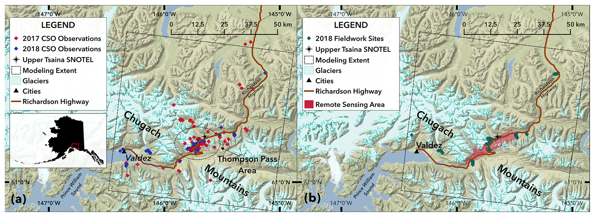
Figure 1Study area map and fieldwork sites. (a) The study area maps showing the CSO measurements, the modeling spatial extent, and the Thompson Pass region of the Chugach Mountains. (b) The 2018 fieldwork includes 72 sites with co-located snow water equivalent and snow depth measurements. The remote sensing data sets from 2017 and 2018 are overlain on the map, along with the location of the Upper Tsaina SNOTEL station.
3.1 Model dataflow
This study relies on a common research design in snow science that uses (1) in situ snow observations, (2) physically based process modeling, and (3) remote sensing of the snowpack to accomplish its primary objectives (Sturm, 2015). Figure 2 is a conceptual diagram of how the citizen scientists' snow depth measurements fit into the model chain for the present study. The modeling process begins with the weather forcing products and citizen scientists' snow depth observations as model inputs. Submodels for meteorological variable distribution, snow depth to SWE estimation, and for the assimilation of snow measurements are employed before the final simulation occurs. The process model outputs are then validated by the RS data sets, the SNOTEL station record, and the 2018 field measurements. Incorporating the citizen scientists' observations into the model chain is an attempt to modify the model outputs by in situ snow depth observations.
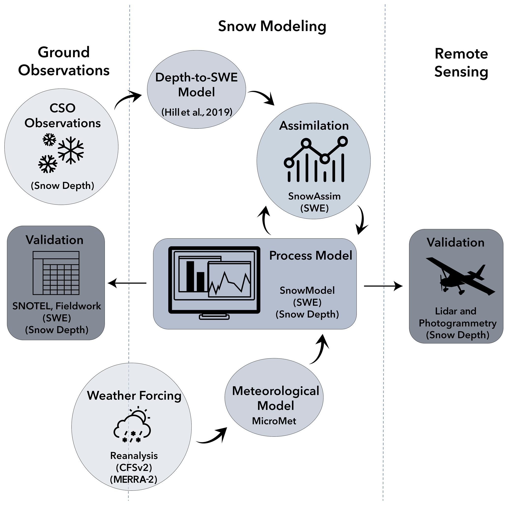
Figure 2Model dataflow diagram. The model chain begins with the weather forcing product and the CSO data sets. The arrows indicate dataflow through the series of submodels to the process model output. The model output is then validated by the SNOTEL station time series, the 2018 fieldwork, and the remote sensing data sets.
3.2 Modeling framework
In this study, we used a sequence of models to simulate SWE and snow depth distributions within the Thompson Pass study area during WY2017 and WY2018. The sections below provide brief information about the models used in this study. For more details, please refer to the source citations for each model.
3.2.1 SnowModel
SnowModel (Liston and Elder, 2006a) is a physically based, spatially distributed process model for simulating the evolution of snowpacks in snowy environments, and has been used for high-resolution and hemispheric-scale modeling worldwide (Beamer et al., 2016, 2017; Crumley et al., 2019; Liston and Hiemstra, 2011; Mernild et al., 2017a, b). We chose SnowModel for the Chugach Mountains study area because it contains a data assimilation submodel, SnowAssim, and a snow transportation submodel, SnowTran-3D. Within SnowModel, various other submodels solve the energy budget for the snowpack, generate runoff quantities, etc. The present study focuses on the snow depth and SWE distribution outputs from SnowModel from simulations with and without the data assimilation submodel.
3.2.2 MicroMet
MicroMet (Liston and Elder, 2006b) is a meteorological distribution submodel for weather station or reanalysis data sets that can be paired with SnowModel in spatially explicit modeling applications. MicroMet uses the Barnes objective analysis scheme for interpolating meteorological input variables to the gridded SnowModel domain for each model time step (Barnes, 1964, 1973). In the present study, instead of using local weather station data, the model is forced with reanalysis data, and MicroMet uses the node locations as weather stations, accessing the reanalysis node surface level precipitation, wind speed and wind direction, relative humidity, air temperature, and elevation variables for the spatial interpolation. MicroMet has been paired with reanalysis weather products and SnowModel in many studies worldwide (Baba et al., 2018; Beamer et al., 2016; Liston and Hiemstra, 2011; Mernild et al., 2017a).
3.2.3 SnowTran-3D
Wind redistribution of snow is an important factor for the spatial distribution of snow depths and SWE distributions for snow modeling (Clark et al., 2011). Wind events build snow deposits in the gullies and the leeward side of bedrock features into drift depths greater than 10 m at times within the Thompson Pass study area. These events also leave some portions of the landscape completely scoured and void of snow, based on fieldwork observations and the RS snow surveys from both years. SnowTran-3D is a submodel within SnowModel that redistributes the snow laterally in the model grid according to the processes that govern snow transportation, namely fetch, wind speed, wind direction, wind shear stress and the shear strength of the snowpack, saltation and turbulent suspension of the snow, and sublimation (Liston et al., 2007). SnowTran-3D is suitable for use as a subroutine within SnowModel when the model grid cell resolution is appropriate for the length scale of snow transportation processes to occur, for example, primarily at model resolutions less than 100 m.
3.2.4 SnowAssim
To assimilate the CSO measurements, we used the submodel SnowAssim developed in tandem with SnowModel (Liston and Hiemstra, 2008). The SnowAssim data assimilation scheme is relatively simple when compared to other assimilation methods. Direct insertion methods often insert the observed state values into the modeled field in the locations and times where data are available (McGuire et al., 2006; Fletcher et al., 2012). Hedrick et al. (2018) outlines a modified direct insertion method, where Airborne Snow Observatory lidar-based snow depth distributions are input into the iSnobal workflow to modify model state variables before a new initialization of the model begins. Liston and Hiemstra (2008) describe a different type of modified direct insertion assimilation scheme (SnowAssim) used in the present study. SnowAssim requires the model to be run twice and pauses at the end of the first model run. During this pause, differences between the observed SWE depths and modeled SWE depths in time and location are calculated and interpolated to the entire model domain in the form of a correction surface. The final correction surface is spatially distributed (for each day of observations) using the Barnes interpolation scheme. These correction surfaces are then applied to the precipitation inputs and snowmelt factors during the second model run.
Note that CSO measurements are submitted as snow depth (meters), but the SnowAssim model code and physical equations require observational inputs to be SWE depth (meters), so a conversion from depth to SWE was necessary. The snow depth to SWE conversion method for the current study will be discussed in the following section. The model determines the dominant snow season phase (accumulation or ablation) and applies the correction factor surface to either (a) the precipitation fluxes or (b) the snowmelt factors during the second model simulation. Additionally, the Barnes interpolation scheme determines outliers within the observed data set and determines the degree to which the assimilated values fit the modeled values. This determination creates a smoothed representation of the observed data set in the assimilation results. For extensive details about the data assimilation scheme, see Liston and Hiemstra (2008; their Sects. 3, 4, and 5).
Other data assimilation methods include the particle batch smoother and particle filters. These are Bayesian data assimilation methods used to estimate system state variables based on predicted estimates (modeled) and noisy measurement data (observed). These types of data assimilation methods rely heavily on characterizing and incorporating the predicted estimate uncertainties and measurement uncertainties into the analysis using probability distribution functions (Magnusson et al., 2017; Margulis et al. 2015). In direct insertion or modified direct insertion methods like SnowAssim, modeled and observed state variable uncertainties are not explicitly characterized.
3.2.5 Snow depth to snow water equivalent conversion
CSO participants take measurements of snow depth, yet SnowAssim requires SWE observation inputs. A conversion from snow depth to SWE was necessary for the present study. A body of research exists on the best methods for converting point measurements from snow depth to SWE, using either bulk density estimations, snow climate classifications, statistical models, or atmospheric conditions and energy balance approaches (Sturm et al., 1995; 2010; McCreight et al., 2014; Jonas et al., 2009; Pagano et al., 2009; Hill et al., 2019; Pistocchi, 2016). The Hill et al. (2019) model was chosen for two reasons. First, the data requirements are minimal for this model, as it requires only location, day of water year (DOY) and readily available climatological information based on input location. These minimal requirements align with the information available from CSO measurements. Second, it was found to outperform other bulk density methods, such as Sturm et al. (2010) and Jonas et al. (2009), when tested against a wide variety of snow pillow and snow course data sets, with an overall bias of 0.2 cm and root mean squared error (RMSE) in SWE of 6 cm (Hill et al., 2019).
3.3 Model input data sets
3.3.1 Elevation and land cover
SnowModel requires a digital elevation model (DEM) and a land cover model as two of the three primary input data sets. The DEM is the National Elevation Dataset (NED) from the United States Geological Survey downloaded at 30 m resolution and then rescaled to 100 m spatial resolution (Gesch et al., 2002). The land cover model is the National Land Cover Database (NLCD) 2011 data set at 30 m spatial resolution and then resampled to 100 m resolution (Homer et al., 2015). The NLCD data set was reclassified to match the land cover input classes required by SnowModel. Initially, we tested results from model simulations at two spatial resolutions, i.e., 30 and 100 m, covering the Thompson Pass model domain. After calibrating the model, the results section only includes the 30 m resolution.
3.3.2 Weather forcing data sets
Various weather reanalysis products have been used in remote portions of Alaska in previous studies (Beamer et al., 2016, 2017; Crumley et al., 2019; Liston and Hiemstra, 2011). In Alaska, each reanalysis product shows bias corresponding to meteorological variable, regional location, and season of the year (Lader et al., 2016; see their Figs. 3 and 4). For this reason, the current study considered two weather reanalysis products that differ in their biases in temperature and precipitation in the Thompson Pass region during the winter and the summer seasons. We used the Climate Forecast System version 2 product (CFSv2) and the Modern-Era Retrospective Analysis for Research and Applications version 2 (MERRA-2) product for the weather forcing inputs for SnowModel. The CFSv2 product from the National Centers for Environmental Prediction is an extension of the lower spatial resolution Climate Forecast System Reanalysis (CFSR) version 1 product that began in 1979, and the version 2 product became available in 2011 (Saha et al., 2010). The CFSv2 data are available at a spatial resolution of 0.2 arcdegree, and a 6 h temporal resolution (Saha et al., 2014). The CFSv2 data set was downloaded using Google Earth Engine (GEE), a platform for accessing and analyzing scientific data sets with global coverage. The MERRA-2 weather reanalysis product from NASA's Global Modeling and Assimilation office is the second meteorological forcing data set tested in the present study (Gelaro et al., 2017). The MERRA-2 data are available at a spatial resolution of 0.667∘ × 0.5∘, with a 3 h temporal resolution, beginning in 1979. MERRA-2 replaces the older version product with updated assimilation processes to include more weather data sets.
3.4 Snow data sets
3.4.1 Snow telemetry station data
The study area contains two SNOTEL stations operated by NRCS. The first station is the Upper Tsaina SNOTEL (UTS) station located at 534 m a.s.l. on the NE side of Thompson Pass, reporting the full standard set of sensor variables, including precipitation, temperature, snow depth, and SWE. The second station is the Sugarloaf Mountain SNOTEL (SLS) station, located near the Valdez Arm of the Prince William Sound at 168 m a.s.l. in the SW corner of the study area, and it records precipitation, temperature, and snow depth but not SWE (Fig. 1). The SLS station data were used to create local temperature lapse rates for the calibration, and the UTS station data were used in Sect. 6 to create the SWE time series analysis. Detailed information about the SNOTEL sensors and climate monitoring instruments can be found at the SNOTEL website (https://www.wcc.nrcs.usda.gov/snow/, last access: 11 August 2021) and in Serreze et al. (1999). Direct links to the SNOTEL websites for the UTS and SLS stations can also be found in the code and data availability section below.
3.4.2 Lidar and photogrammetry-derived data
An aerial photogrammetric survey was conducted on 29 April 2017 with a Nikon D800 36.2 MP (megapixel) camera flown on a fixed-wing aircraft above a portion of the Thompson Pass study area (see Fig. 1b for location and extent). An onboard Trimble Global Navigation Satellite System (GNSS) and a base station were used for positional control. Post-processing was completed with structure-from-motion software to create a digital surface model (DSM) of the photogrammetry-derived snow surface. An airborne lidar survey was collected on 7 and 8 April 2018, using a RIEGL VUX1-LR laser scanner flown on a fixed-wing aircraft. An onboard integrated inertial measurement unit (IMU) and GNSS and a base station were used to provide positional control for the lidar-derived snow DSM. Both RS data sets were evaluated against a previously collected photogrammetry-derived DSM from 2014 when no snow was present. An interpolation scheme was used to gap-fill some of the negative values in the snow DSM due to vegetation cover effects. There is uncertainty associated with the RS data set acquisitions, and the sources of error are related to flight trajectory and geometry, laser scan angle, density of vegetation and canopy, and steep gradients in the terrain (Deems and Painter, 2006). The vertical RMSE in snow depth for the photogrammetry and lidar data sets are estimated at 31.0 and 10.2 cm, respectively. While we acknowledge and report these error estimations, they are integrated into the results in Table 3 (see Sect. 6.5) but not used in the spatial results reported in Sect. 6.2.
3.4.3 Chugach 2018 fieldwork data
In total, 3 weeks of fieldwork in the Thompson Pass region were conducted in March–May 2018. Snow depth and SWE were measured throughout the study area with an avalanche probe and a Federal snow sampler. At each fieldwork measuring site, a central SWE measurement was taken using the Federal sampler. Avalanche probes were used in the surrounding 100 m2 to take a series of eight snow depth measurements extending 5 m in each direction from the central SWE measurement. Federal sampler data collection introduces uncertainty in the form of measurement error due to variable snow conditions and densities, hard impenetrable crusts, and loss during extraction. Dixon and Boon (2012) report the results of several studies, showing that the Federal sampler error, as a percentage of SWE depth, ranges from 4.6 % to 11.2 %. Our results (presented in Sect. 6.5) include field measurements of SWE that use the higher 11.2 % value for conservative SWE error estimation.
The fieldwork sampling protocol was designed to consider (1) variability in snow depth in small areas less than 100 m2, (2) month-to-month changes in snow depth and SWE, and (3) spatial gradients in snow density throughout the entire study area. A diagram of the location of each observational site can be found in Fig. 1b. The 2018 fieldwork data set was used for validation with two purposes in mind. First, the 2018 fieldwork SWE measurements were used as a validation data set for the 2018 SWE distribution results. Second, since the data collected in the spring of 2018 contains measured snow depths and SWE at 70 observational sites (n= 560; eight per site), we conducted an analysis of the subgrid-scale variability in snow depth found at each observational site, and these results are found in the Sect. 7.
3.4.4 Community Snow Observations data
The CSO program collects snow depth data from citizen scientists in snowy environments worldwide. Full details, including links to smartphone apps and tutorials, are found at http://communitysnowobs.org (last access: 11 August 2021). Citizen scientists take several (2–4) snow depth measurements within a small area (< 4 m2) using an avalanche probe or other depth measuring device (meter stick, etc.). These measurements are then averaged by the participant and submitted using the app or program preferred by the participant. The submitted data include the global positioning system (GPS) location in latitude and longitude, time and date, and snow depth measurement (centimeters). The accuracy of the GPS system for each participants' mobile device determines the location error of the GPS, with common errors for mobile phones ranging between ±4 and 7 m (Garnett and Stewart, 2015; Schaefer and Woodyer, 2015). Since the model resolution is 30 and 100 m, this level of horizontal error in GPS location is acceptable for the purposes of our research questions. All collected data are made freely available on the CSO website for visualization and download (see data availability at the end of the paper). In total, thousands of measurements have been recorded by participants in CSO globally since it began in January 2017 with initial measurement campaigns in Alaska and other frequently visited locations in mountain regions across North America (Fig. 3). In the modeling domain of the current study, 442 CSO measurements were available for WY2017 (water year 2017) and 104 CSO measurements for WY2018 (water year 2018). These measurements were concentrated in the Thompson Pass region of the study area (Fig. 1) and range from 25 to 1400 m in elevation.
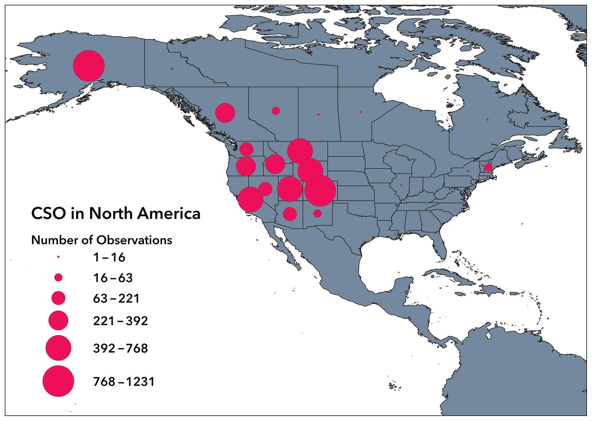
Figure 3CSO participation in North America. Participation in the CSO project in North America aggregated by the number of observations recorded in each USA state or Canadian province between 1 January 2017 and 31 December 2019.
We performed model calibration using 5 years of the historical record of the UTS station from WY2012 (water year 2012) through the end of WY2016 (water year 2016). The calibration was focused on adjustments to temperature lapse rates, precipitation lapse rates, wind adjustment factors, and the use of the SnowTran-3D submodel. We chose temperature lapse rates and precipitation lapse rates for calibration because SnowModel is known to be limited by these factors when large elevational differences exist within the model domain (Liston and Elder, 2006a). We chose wind adjustment factors and the wind transportation submodel for calibration because the wind redistribution of snow plays a significant role in the study area, based on the 2018 fieldwork and the RS surveys from 2017 and 2018. Since the SnowAssim submodel requires a single layer snowpack, no adjustments were made to the snowpack layer structure. For each weather reanalysis product, a full calibration was performed for the 30 and 100 m model resolutions in the event that spatial resolution plays a significant role in parameter selection. See Appendix A for the descriptions of the model parameters tested during the calibration.
The daily SWE output from each calibration simulation is compared with the UTS observed SWE for the duration of the 5-year calibration time period using the root mean squared error (RMSE), the Nash–Sutcliffe efficiency (NSE), the Kling–Gupta efficiency (KGE), and mean bias error (bias) to assess the calibration simulations. Table 1 lists the best 30 and 100 m calibration simulations based on their time series RMSE, NSE, KGE, and bias scores. We acknowledge that measurement errors can occur with SNOTEL snow pillows, and that these well-known errors may affect the accuracy of the observational data set (Johnson and Schaefer, 2002; Johnson, 2003).
Table 1Model calibration results. The best calibration results are given for each set of simulations for water years 2012–2016, along with the root mean squared error (RMSE), the Nash–Sutcliffe efficiency (NSE), the Kling–Gupta efficiency (KGE), and the mean bias error (bias).
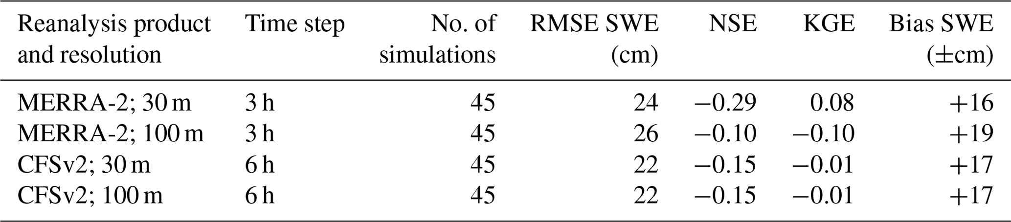
Calibration results in Table 1 show that the 30 m model grid resolution slightly outperforms the 100 m model grid resolution in the MERRA-2-forced calibration simulations. However, the CFSv2-forced simulations show no difference between the model grid resolutions. The CFSv2 product slightly outperforms the MERRA-2 product in terms of SWE RMSE. Overall, the differences between the top-performing model grid resolution and reanalysis product are mixed and potentially negligible, varying by metric. The NSE and KGE model performance metrics in the calibration simulations are lower than expected, due primarily to precipitation inputs from the reanalysis products that were consistently higher than measured precipitation at the UTS station (see the following paragraph for more details). The SnowModel default parameter values notably and consistently produce the top performing simulations, see Appendix B for details. Due to each of these factors, the calibrated model for the remainder of the study uses the CFSv2 reanalysis product, the 30 m model grid resolution, and the SnowModel default parameter values.
One of the primary obstacles for process modeling is the availability of accurate weather input data, and the related uncertainties with weather inputs are a well-known complication in snow and hydrological modeling (Rivington et al., 2006; Schmucki et al., 2014; Schlögl et al., 2016). Initial tests of modeled precipitation fields using MicroMet versus the observed precipitation at the UTS station revealed that both reanalysis products overestimated the amount of precipitation observed in the study area at the UTS station (see Appendix C). The CFSv2 precipitation totals at the UTS station were nearly 1.6 times the measured precipitation at the UTS station during the calibration period. The improvements that could be gained by adjusting a subset of the model parameters (wind, temperature, and precipitation lapse rates due to differences in elevation and season) during calibration were not likely to overcome this extreme precipitation deficiency, explaining why the final calibrated NSE and KGE values were low. There are two ways to address this precipitation deficiency using SnowAssim. One is to adjust the precipitation inputs during calibration, and the other is to allow the assimilation to adjust the precipitation inputs. Both ways are functionally equivalent because they apply a simple, scalar-based correction surface to the precipitation fluxes. In our calibration process, we chose to use SnowAssim to address the precipitation deficiencies in the reanalysis product, following the approach of other recent studies in mountainous regions of Alaska and following the original purpose of the SnowAssim model (Cosgrove et al., 2021, and their Calibration of SnowModel section; Liston and Heimstra, 2008; Young et al., 2020, and their Sect. 3.4). This calibration decision supports the primary goal of the current study, which is to test whether or not participant-submitted snow depth measurements can improve physically based modeling efforts through data assimilation.
These calibration results and the precipitation deficiencies motivated us to design an experiment to supplement the main findings of this research. For this experiment, we introduced a model precipitation adjustment factor similar to the method outlined in Mernild et al. (2006). We applied this scalar value to the precipitation fields as a bias correction of the precipitation inputs. We tested 11 precipitation adjustment factors ranging from 0.95 to 0.45 and applied them to the meteorological forcing inputs during the 5-year calibration time period. For more details about the precipitation and precipitation adjustment factor results, see Appendix D. This experiment, with a summary of the results presented in Sect. 6.6, allows us test improvements in model performance when the precipitation inputs are bias-corrected prior to model assimilation of CSO measurements.
We carried out a series of simulations in order to (1) quantify the improvement in model performance due to the assimilation of CSO measurements and to (2) understand the effects of the number of CSO data points selected for assimilation. First, we set up geographic and temporal requirements for the assimilated data. The only geographic requirement was that the CSO measurements must be located within the larger 5736 km2 model domain. We subset the CSO measurements temporally to the peak SWE time period or later. According to the UTS station, peak SWE in the study area generally occurs mid- to late April, and consequently, the earliest assimilation date was set to 15 April. The CSO measurements were aggregated by week by assuming all measurements in a given week occurred on the same day for the purposes of assimilation. This weekly aggregation allows the correction surfaces generated by SnowAssim time to adjust the precipitation fluxes and snowmelt factors between observations, thereby altering the model outputs during assimilation. Additionally, CSO participation in the Thompson Pass region during the early accumulation season was infrequent in WY2018 and nonexistent in WY2017. Since peak SWE is important for mountain hydrology and ecology, with many snow studies using it as an indicator metric, the time restrictions are acceptable for the research questions addressed in this study (Bohr and Aguado, 2001; Trujillo et al., 2012; Kapnick and Hall, 2012; Mote et al., 2018; Wrzesien et al., 2017).
With these geographic and temporal filters defined for assimilation, we decided to vary the number of CSO data points selected for assimilation. Model simulations without CSO measurements provide a baseline for comparison, referred to as the NoAssim case. Ensemble model simulations were carried out with various numbers of CSO measurements assimilated, referred to as the CSO simulation case. An ensemble of 60 trials per year were carried out with n= 1, n= 2, n= 4, n= 8, n= 16, and n= 32, where n equals the number of CSO measurements assimilated per WY. In each instance (n value), 10 realizations of the numerical experiment were carried out. With the ensemble model simulations defined in terms of the spatial and temporal restrictions, the number of CSO measurements was the only feature modified during assimilation.
The following results reflect the three types of available validation data sets: (1) time series SWE results at the UTS station, (2) spatial snow depth distributions from the RS data sets, and (3) point-based snow depth and SWE measurements from the 2018 fieldwork.
6.1 Temporal results using the Upper Tsaina SNOTEL station
The temporal results compare the UTS station SWE time series to the ensemble member SWE time series during WY2017 and WY2018. Figure 4 displays the temporal cycle of snowpack accumulation and ablation, and the timing of peak SWE. At the UTS station in the study area, the average WY day of peak SWE is 228 or 15 April. Before this day, the snowpack is generally increasing in SWE, and afterwards the snowpack generally enters the ablation period with a reduction in SWE. This temporal cycle can be observed in Fig. 4 by following the color gradient. The highest-performing (best) CSO simulation (Fig. 4b, e) corrects the slope of the snowpack accumulation and ablation phases when contrasted with the NoAssim accumulation and ablation phases and slopes (Fig. 4a, d). These time series results, in terms of model performance metrics and the snowpack temporal cycle, exhibit SnowAssim's ability to incorporate CSO measurements and improve modeled SWE outputs at the UTS station location throughout the entire snow season.
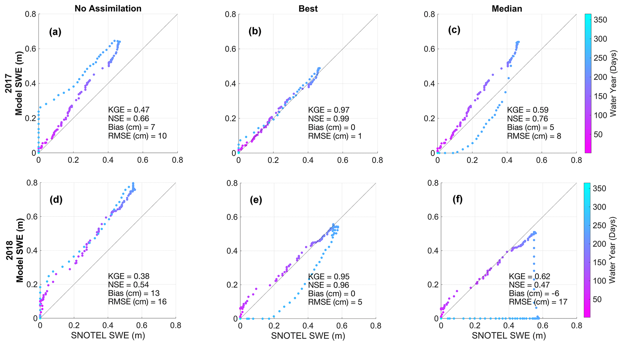
Figure 4Time series at Upper Tsaina SNOTEL station. The Upper Tsaina SNOTEL snow water equivalent (SWE) observations versus the modeled SWE for the no assimilation case (a, d), the best CSO simulation (b, e), and the median CSO simulation (c, f). The time series color gradient corresponds to the day of the water year.
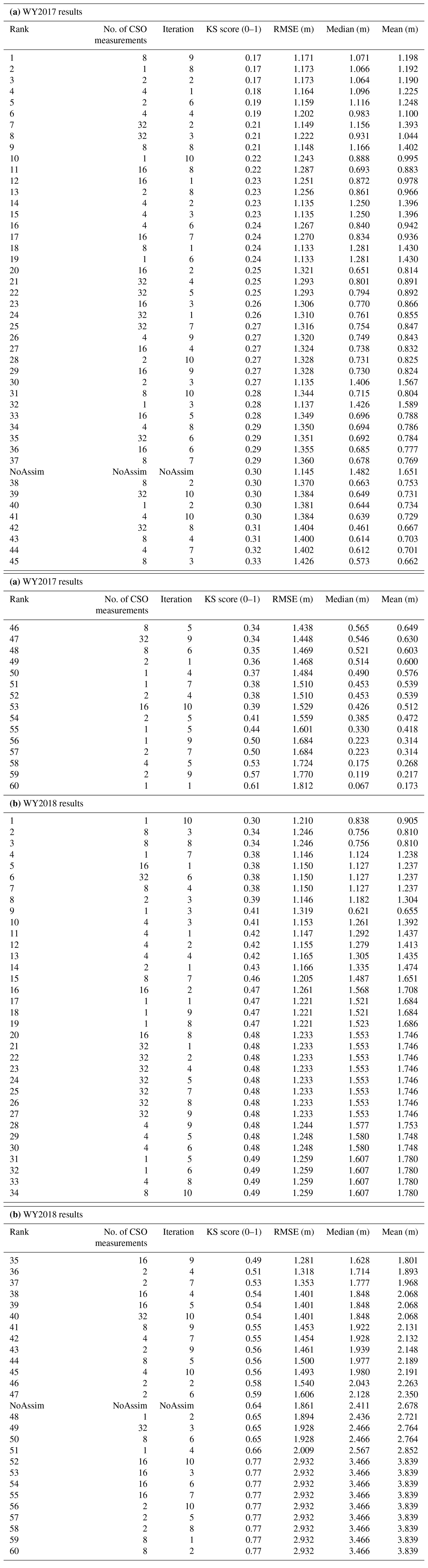
Figure 4 summarizes the temporal results for the best and median performing (median) CSO simulations, as well as the NoAssim case. Each ensemble member is evaluated by their KGE, NSE, RMSE, and bias scores. For results presented in this section, the KGE score is used to rank the ensemble simulations. A full accounting of each ensemble member and their time series ranking can be found in Appendix E. Modeled SWE depths for the NoAssim case are consistently higher than the UTS station SWE observations for both WYs (Fig. 4a, d). The modeled SWE depths for the best CSO simulation outperform the NoAssim case throughout the entirety of the time series and represent an improvement in model performance scores according to all of the time series metrics (Fig. 4b, e). The modeled SWE depths for the median CSO simulation for WY2017 outperform the NoAssim case by all metrics, and the WY2018 median CSO results are mixed. The ensemble simulation KGE scores outperform the NoAssim KGE scores among 70 % of the WY2017 ensemble members, and among 67 % of the WY2018 ensemble members. Any number of CSO measurements assimilated show improvements in model performance, which is a key finding in the time series results.
Using the snow depth to SWE conversion method during assimilation introduces uncertainty into the modeling process. Instead of using the global estimates of error reported in Hill et al. (2019; RMSE in SWE = 5.9 cm) we decided to calculate this source of error using our fieldwork site measurements. The RMSE in SWE due to the conversion method is 10.5 cm, and we perturbed the CSO observations by this amount to depict the upper and lower boundaries of error associated with this source of uncertainty. Figure 5 displays the best CSO simulation temporal results for each WY, along with the UTS station SWE record and the NoAssim case. These perturbations to the assimilated SWE show improved modeled SWE values at the UTS station when compared to the NoAssim case, even after this source of uncertainty has been accounted for.
Since the timing of snow disappearance is important for ecological systems in alpine environments and water resources managers, we calculated the range in snow disappearance dates from the best simulations from both water years (see Fig. 5, where SWE depth reaches zero between days 250 and 280). In WY2017 and WY2018, the snow disappearance date for the NoAssim case is 10 and 7 d later than the UTS station record, respectively. In WY2017, the snow disappearance date in the best CSO simulation, accounting for measurement uncertainty, ranges from 3 d earlier to 8 d later than the UTS station. In WY2018, the range is from 10 to 1 d earlier than the UTS station. These ranges in snow disappearance date are acceptable and show improvements in model performance for some, but not all, of the best CSO simulations after accounting for measurement uncertainty.
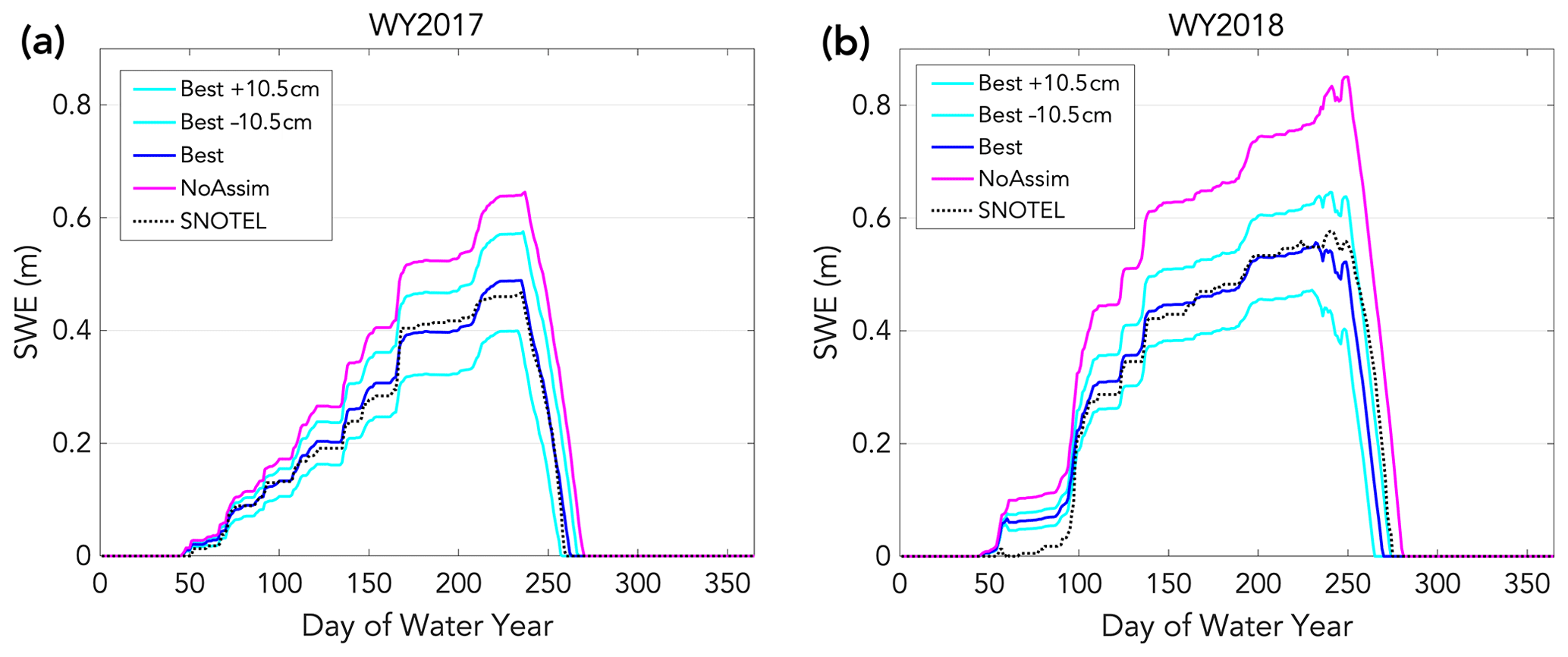
Figure 5Snow water equivalent (SWE) time series results with measurement uncertainty included. The simulations with ±10.5 cm of SWE represent the upper and lower boundaries of error introduced when converting snow depth measurements to SWE using the Hill et al. (2019) method.
6.2 Spatial results using the remote sensing data sets
The ensemble results are summarized in Fig. 6 using the Kolmogorov–Smirnov statistic (KS; Massey, 1951). The KS statistic quantifies the difference between a reference data set of a continuous variable and a sample data set of the same variable. The KS statistic represents the maximum distance between the empirical cumulative distribution function (ECDF) of the reference and sample data sets, with KS scores ranging from 0 to 1, with 0 representing perfect data set agreement (Riemann et al., 2010). In the KS analysis, the reference data set is the RS-derived snow depth distribution, and the sample data sets are each of the ensemble snow depth distributions, including the NoAssim case. Figure 6 shows that in WY2017 the CSO simulations are an improvement from the 2017 NoAssim case among 62 % of the ensemble members and in WY2018 among 78 % of the ensemble members. Note that only the KS values that fall below the NoAssim line represent an improvement in model performance during the CSO simulations. The spatial results reveal that improvements in model performance are not dependent upon the number of CSO measurements that are assimilated in WY2018. However, WY2017 has a smaller range in KS values as the number of assimilated measurements increases, with more CSO simulations outperforming the NoAssim case. However, WY2017 has a smaller range in KS values as the number of assimilated measurements increases. Additionally, the number of simulations that outperform the NoAssim case in WY2017 gradually increases as the number of CSO measurements increases from 1 to 32. These results also vary according to model performance metric and by WY, with no clear pattern emerging from the number of measurements assimilated.
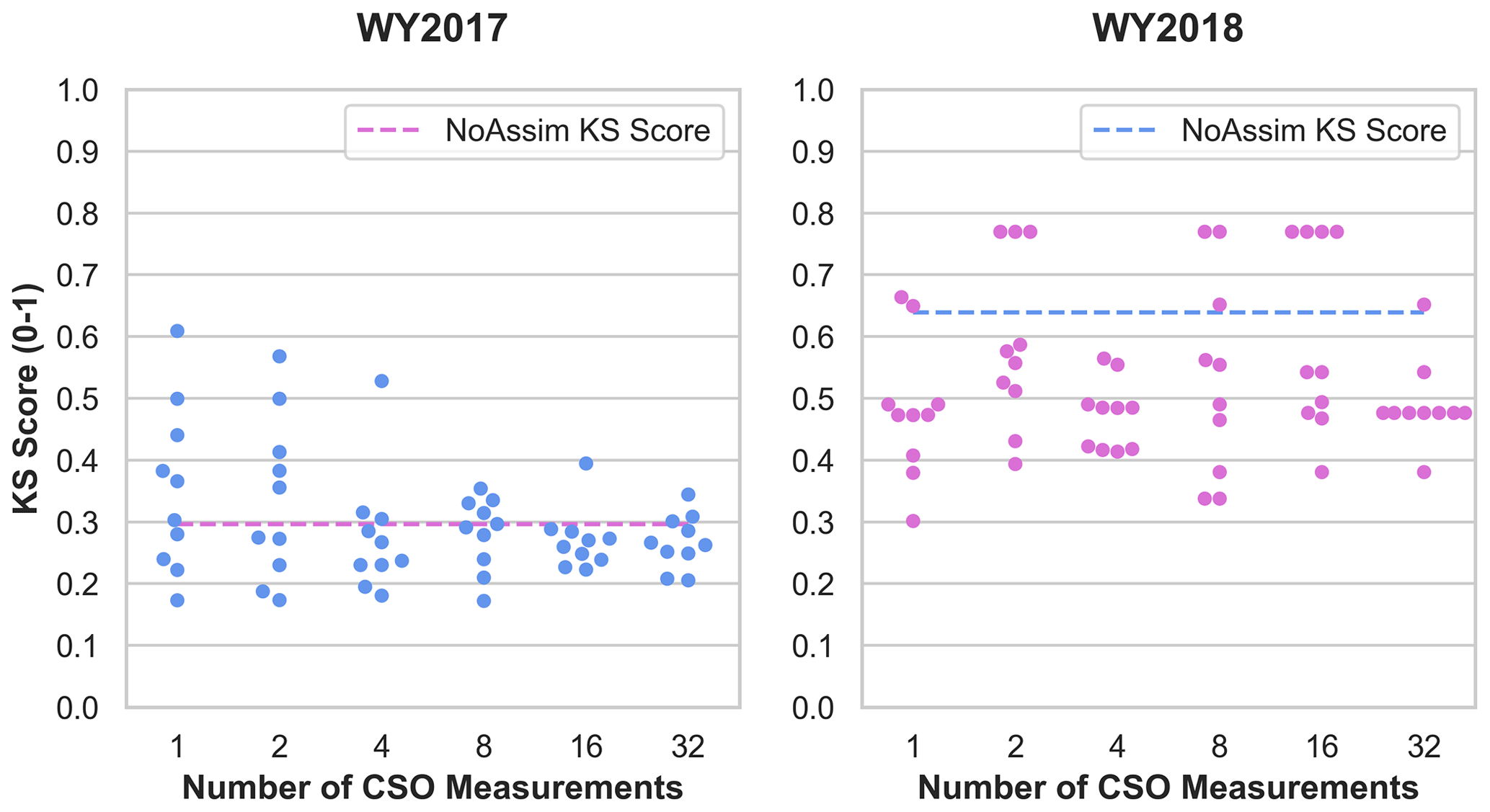
Figure 6Swarm plots of Kolmogorov–Smirnov scores. The ensemble simulations are ranked by Kolmogorov–Smirnov (KS) score per year and plotted according to the number of measurements assimilated, including the no assimilation (NoAssim) case.
The snow depth distribution maps in Fig. 7 display the RS data sets (Fig. 7a, b), the results from the best CSO simulation (Fig. 7c, d), and the NoAssim case for each WY (Fig. 7e, f). Refer to Fig. 1 for the RS data set location within the study area. We present the best CSO simulation as the focus of Sect. 6.2 and ranked according to KS score ranking (Fig. 6). A full accounting of each ensemble member and their spatial distribution ranking can be found in Appendix F. In the RS data sets, there is more variation and heterogeneity in snow depth across short distances (Fig. 7a–b). This spatial diversity is evident even after the RS data set has been aggregated to correspond to the model resolution at 30 m, as depicted in Fig. 7. The NoAssim case and best CSO simulation show less spatial diversity, and the NoAssim case broadly overestimates snow depth when compared to the Best CSO simulation for both WYs. The visualization of the snow depth distributions in Fig. 7 illustrates the challenges of accurately representing the process scale through physics-based modeling at low resolutions (Blöschl, 1999), and some of these challenges will be examined further in the discussion section.

Figure 7Snow depth distribution maps. (a, b) The remote sensing (RS) data sets from 2017 and 2018. (c, d) The best CSO simulation results corresponding to the RS data set spatial extent. (e, f) The no assimilation results corresponding to the RS data set spatial extent. The total model area that corresponds to the RS data set in 2017 is 104 km2, and in 2018 it is 149 km2.
Figure 8 presents histograms and empirical cumulative distribution functions (ECDFs) for the RS data sets, the NoAssim case, and the best CSO simulation. In WY2017 (Fig. 8a), when the NoAssim case overestimates snow depths, the best CSO simulation ECDF shifts left, towards the RS data set ECDF. To a greater degree, in WY2018 (Fig. 8c) when the NoAssim case more broadly overestimates the snow depths, the best CSO simulation ECDF shifts further left, towards the RS data set ECDF. The shifts in the EDCFs are evident in the histograms, and the median value of each data set is indicated with a dashed line (Fig. 8b, d). The same shifts are evident in the snow depth distribution maps (Fig. 7c, d, e, f). Even though the shifts in ECDFs and histograms are in the correct direction in the best CSO simulations, SnowAssim is not adjusting the distribution of snow depth values, which can be seen in the multimodal shape of the histograms.
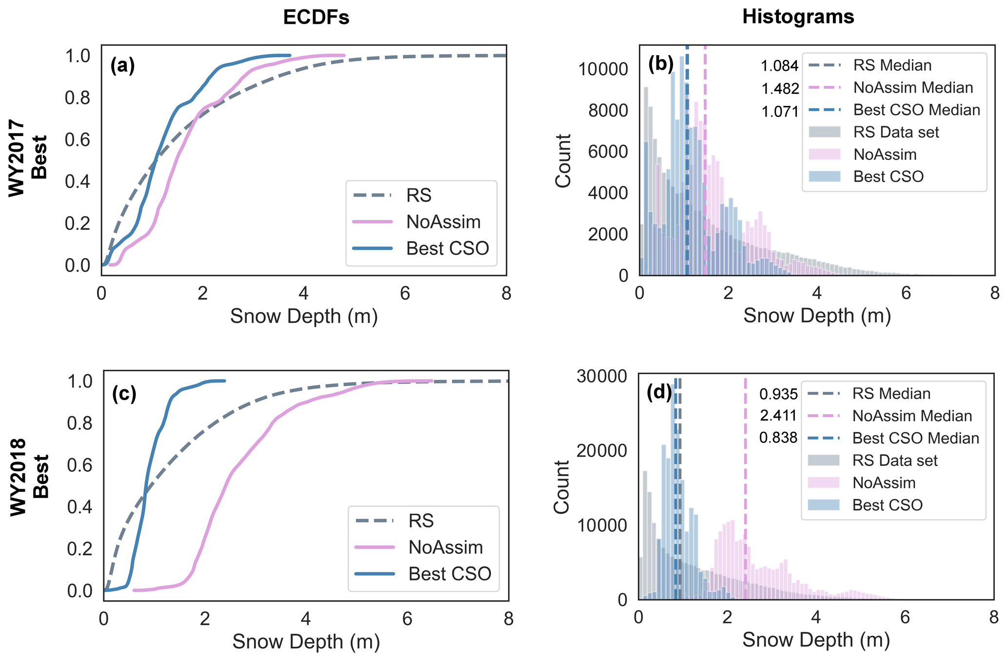
Figure 8Histogram and distribution plots. The empirical cumulative distribution functions (ECDFs) and histograms from the best CSO simulation, the no assimilation case, and the remote sensing (RS) data sets during WY2017 (a, b) and WY2018 (c, d).
The multimodal distribution of snow depths in the modeled results can be explained by their relationship to the elevation of the surrounding terrain. The input DEM and the snow depth distributions were compared on a grid-cell-to-grid-cell basis using a two-dimensional histogram (2DH). Figure 9 is a series of 2DHs that display snow depth (x axes) versus the input DEM (y axes) in the RS area from both years. Darker colors indicate a higher frequency of snow depth and elevation values corresponding to each data set. The 2DHs show a proportional relationship between the modeled snow depths (Fig. 9a, b, e, f) and the input DEM values. As elevation increases, snow depth also increases linearly in the modeled results. Still, the range of snow depths from best CSO simulation shifts towards the RS data set in both years, but the elevation relationship remains largely intact. The RS snow depths are less dependent on elevation, with snow depth values between 0 and 1 appearing at all elevations between 0 and 1250 m. The 2DH analysis supports the findings from the snow depth distribution maps where the variability in the snow depth observed in the RS data set is not replicated in the NoAssim case or the best CSO simulation (Fig. 7).
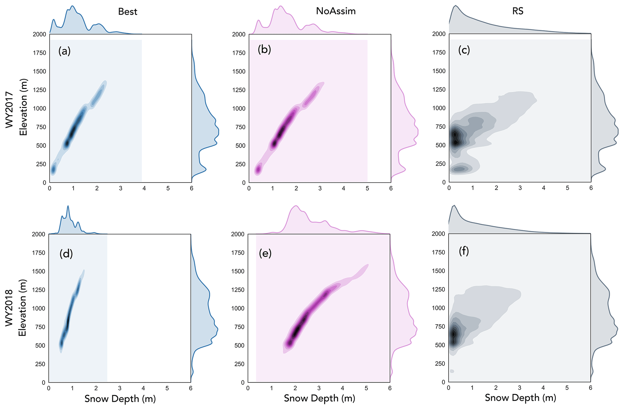
Figure 9The 2D histograms showing the elevation data set vs. the (a) water year (WY) 2017 best assimilation case, (b) WY2017 no assimilation case, (c) WY2017 RS data set, (d) WY2018 best assimilation case, (e) WY2018 no assimilation case, and (f) WY2018 RS data set.
6.3 Spatial and temporal characteristics of the assimilated data
The geographic locations of the CSO measurements used in the temporal and spatial results are an important factor that can shed some light on our understanding of the assimilation process. First, the time series analysis validation metrics were quantified for all days in the water year at the UTS location. The CSO measurements that were assimilated in 2017 range in distance from 4.1 to 30.5 km away from the UTS location, while the best CSO simulation measurements (n= 2) were located 5.5 and 6.9 km away. In 2018, the assimilated measurements range in distance from 2.1 to 17.4 km away from the UTS location, and the best CSO simulation measurements (n= 2) were located 9.1 and 17.5 km away. Figure 10 includes a map of the assimilated measurements and a histogram of the distance between the CSO measurements and the UTS station from both water years, subset by the assimilation time period (on or after 15 April of each year). This distance analysis demonstrates that the CSO measurements used in the time series assimilation do not coincide with the SNOTEL grid cell location. The histogram shows that improvements made at the SNOTEL location during assimilation were due to snow depth measurements taken by CSO participants kilometers away.

Figure 10Assimilated measurements. (a) A histogram showing the distance between the CSO measurements available for assimilation and the Upper Tsaina SNOTEL station, subset by the assimilation time period, on or after 15 April (n= 266). A kernel density estimator is used to smooth the distribution. (b) A map of the CSO measurement locations that includes the best spatial and temporal CSO simulations for both water years. The map is magnified on the area of the highest density of CSO measurements.
Second, the remote sensing data sets were collected on 29 April in 2017 and 7 and 8 April in 2018. These validation data sets are essentially a spatial snapshot of snow depth from a single day in both water years. In water year 2017, there were a total of nine CSO measurements submitted on 29 April, which is the same day as the remote sensing data set collection. For the presented results in Sect. 6.2, none of these nine CSO measurements from 29 April were used. For water year 2018, the remote sensing data set was collected on 8 April, and the measurements were not assimilated temporally until at least 15 April (see the experimental design outlined in Sect. 5). Figure 10b displays the locations of the CSO measurements assimilated in the best CSO simulation from both water years (WY2017 n= 1; WY2018 n= 8). This analysis of the assimilated data demonstrates that the CSO measurements used in the spatial assimilation do not coincide with the dates of the remote sensing acquisition, revealing that improvements were made during assimilation by measurements that were taken at a different time.
6.4 Fieldwork results 2018
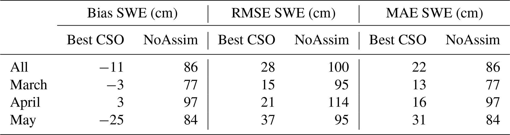
To validate the WY2018 SWE distributions from the NoAssim case and the best CSO simulation, we used ground truth data from our field campaign in April 2018. The locations of the 70 SWE and snow depth measurement sites from 2018are depicted in Fig 1b. Figure 11 shows the co-located SWE depth measurements (y axes) versus the snow depth measurements (x axes) from each site aggregated by month. The bars in Fig. 11 represent the variability in snow depth within the surrounding 100 m2 of the SWE measurement, including the average, minimum, and maximum of eight snow depth measurements at each site. Table 2 shows the results at the SWE measurement sites, comparing the NoAssim case versus the best CSO simulation using RMSE, bias, and mean absolute error (MAE) metrics for evaluation. Since each measurement site corresponds to a single CSO snow depth submission, we separated those measurement sites used in the assimilation scheme from the validation set when creating Table 2. The best CSO simulation outperforms the NoAssim case according to all metrics in all months. The 2018 fieldwork results from April show that the best CSO simulation has a bias of +3 cm, while the NoAssim case is +97 cm. The April 2018 fieldwork results agree with the histogram and ECDF analysis that displayed a broad overestimation of SWE in the NoAssim case in WY2018 (Figs. 7b, 8d).
Additionally, we used the co-located snow depth and SWE measurements at the fieldwork sites to quantify the uncertainty that is added to the model during the snow depth to SWE conversion. By converting the fieldwork snow depth values to SWE using the Hill et al. (2019) method, we can compare the measured SWE to the approximated SWE values. The fieldwork-measured mean SWE is 51 cm, the RMSE in SWE is 10.5 cm, and the bias in SWE is 0.6 cm when using the Hill et al. (2019) method for all fieldwork sites.
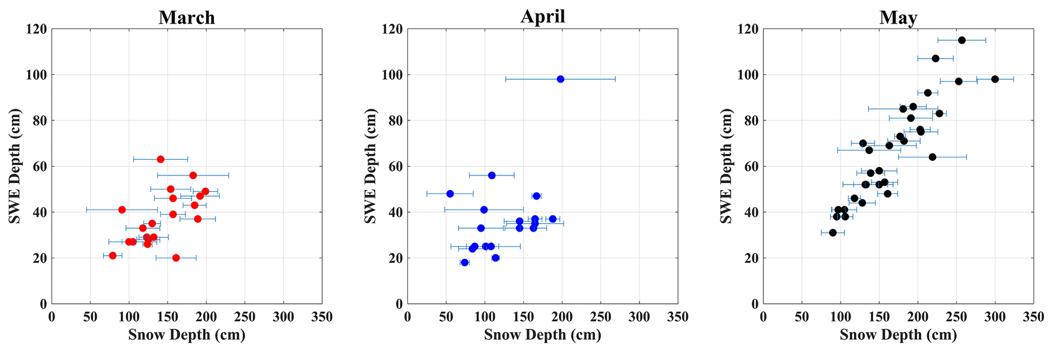
Figure 11Fieldwork 2018 measurements by month. The 70 in situ snow water equivalent (SWE) measurements (y axes) from 2018 are plotted by month, along with their co-located snow depth measurements (x axes). The bars show the minimum, maximum, and average of each fieldwork site where eight snow depth measurements were obtained in a 100 m2 area.
Table 2Fieldwork results 2018. The 70 SWE measurements from the 2018 fieldwork compared to the best CSO simulation and the no assimilation (NoAssim) case using the three model performance metrics, i.e., root mean squared error (RMSE), mean bias error (bias), and mean absolute error (MAE).
6.5 Spatially averaged snow water equivalent results
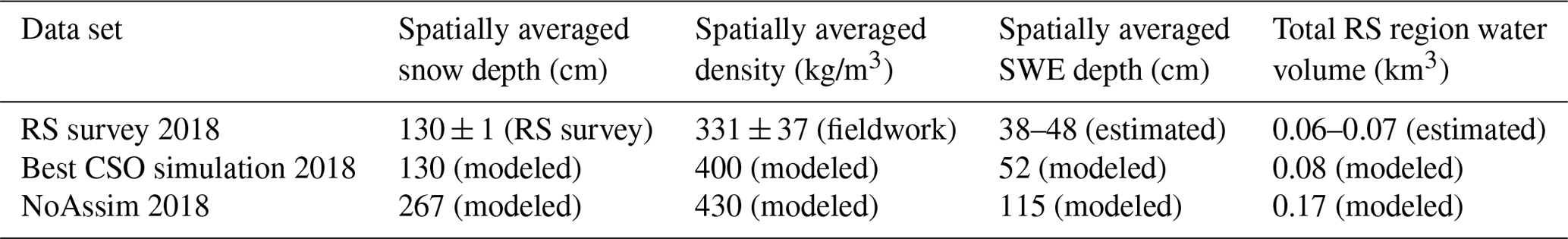
Another way to quantify the ability of CSO measurements to constrain SnowModel output is to investigate the modeled SWE averaged over a large area. Table 3 contains the spatially averaged SWE estimations from the RS survey area in WY2018 and includes the RS data set, the best CSO simulation, and the NoAssim case. We focus on WY2018 because the fieldwork measurements include estimated bulk density values at each measurement site. These bulk density estimations were measured during April 2018 and were partitioned from the larger data set and spatially averaged over the RS region only (n= 22). The fieldwork-estimated bulk density value was then applied to the spatially averaged RS snow depth. The uncertainty estimations for the RS survey data set and the Federal-sampler-collected data are also added to Table 3 to create a range of estimation of water volume. For the best CSO simulation and the NoAssim case, the spatially averaged snow depth, SWE, and snow density values were taken directly from the model results. The SWE estimation results in Table 3 demonstrate that SnowAssim can constrain the SWE output over a large region based on a few, randomly chosen CSO measurements. Importantly, the accuracy of the total modeled water volume from the RS region in 2018 improves when CSO measurements are included, a key finding that has implications for water resource management decisions in snowy, data-limited, mountain environments.
Table 3Spatially averaged variables in the RS region. The spatially averaged results were calculated using the RS region in WY2018, the RS data set (±1 cm error), the spatially averaged density, and the modeled results. The spatially averaged SWE depth for the RS survey was estimated using the average density (±11.2 %) measured during April 2018 fieldwork.
6.6 Precipitation adjustment experiment
The experimental design of the present study was developed for remote locations where a long-term precipitation data set was not available to bias correct the precipitation inputs. However, since a long-term precipitation data set may be available in other locations, we decided to test the results with a precipitation experiment. In this experiment, we applied a scalar to the CFSv2 precipitation fields for bias correction, and all other model parameters and input data sets were held constant. The experiment results show that some of the CSO ensemble simulations still outperformed the NoAssim case with the precipitation adjustment, both spatially and temporally. For example, the spatial results show that 43 % percent of the ensemble runs in WY2017 and 20 % of the ensemble runs in WY2018 outperformed the NoAssim case when the precipitation was bias corrected, according to their KS score (Fig. 12). Similarly, the temporal results show that 42 % of the ensemble runs in WY2017 and 58 % of the ensemble runs in WY2018 outperformed the NoAssim case when the precipitation was bias corrected, according to their KGE score. The ECDF and histogram analysis from the precipitation adjustment factor experiment also show model improvements when there was broad underestimation of snow depths in the NoAssim case in WY2017 and broad overestimation in WY2018. These results demonstrate that using CSO measurements for assimilation can improve model performance when the available weather forcing data set has known biases (no precipitation adjustment factor case), but when those biases have been decreased (precipitation adjustment factor case), the improvements become less clear, they vary from year to year, and are less consistent between spatial and temporal results.
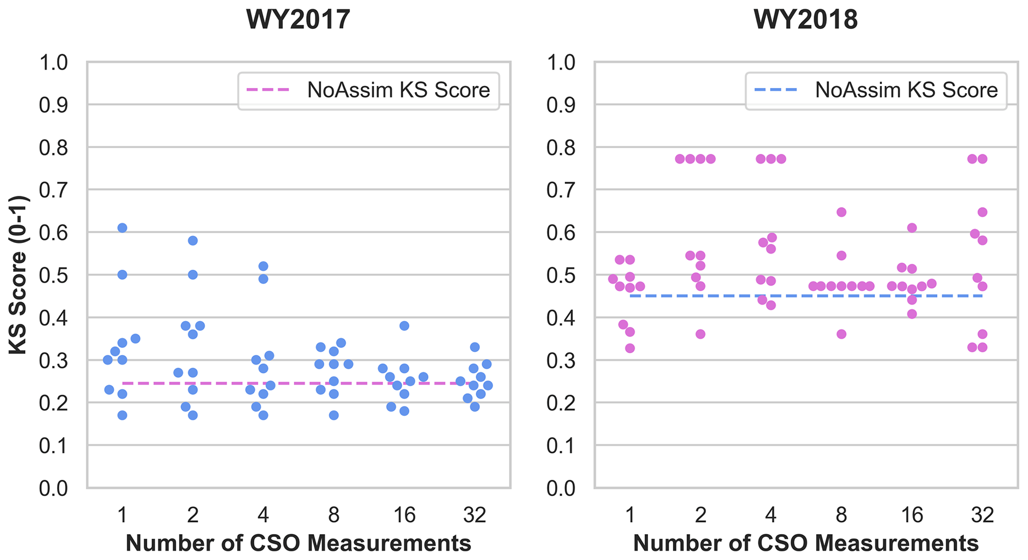
Figure 12Swarm plots of Kolmogorov–Smirnov scores with precipitation adjustment factor. The ensemble simulations are ranked by Kolmogorov–Smirnov (KS) score per water year (WY) and plotted according to the number of CSO measurements assimilated, including the no assimilation (NoAssim) case.
6.7 Correction factor results
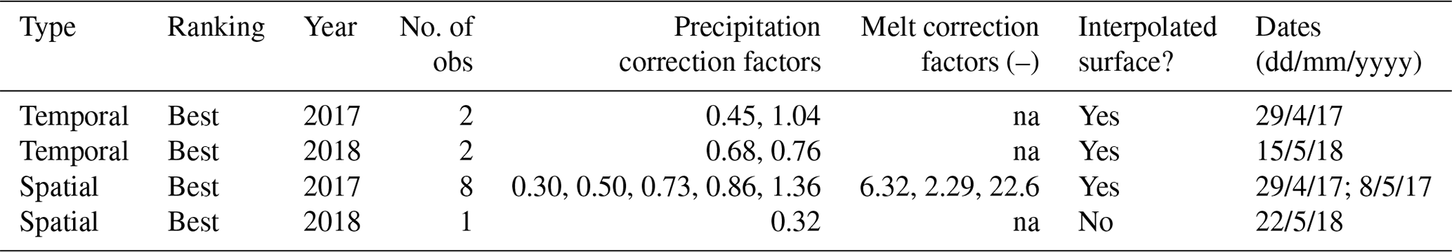
SnowAssim generates a set of correction factors for each of the CSO ensemble member simulations. These factors correspond to the observed and measured differences in the SWE variable and are used to create a correction surface with the Barnes objective analysis. Table 4 reviews a subset of the correction factors, including data from the best-ranked CSO simulations according to the various temporal and spatial metrics previously reviewed in Sect. 6.1 and 6.2. The number of observations varies for the best-ranked simulation and the precipitation correction factors, the use of a melt correction factor, and whether an interpolated correction surface was created. These correction factor results show that relatively few measurements are needed during assimilation, and that there are multiple paths to improving model performance when assimilating CSO observations using SnowAssim.
Table 4Correction factors from the assimilation scheme for the best-ranked simulations from both water years. The model determination for precipitation vs. melt correction factors is included and whether the Barnes objective analysis created a spatially distributed correction surface. Note: na – not applicable.
An important consideration in the results of the present study involves ranking the CSO ensemble members by various spatial and temporal metrics. The time series results (Sect. 6.1), the spatially distributed results (Sect. 6.2), and the spatially averaged results (Sect. 6.5) did not have the same ranking order for the CSO ensemble members. For example, the best CSO simulation in WY2017 from the time series analysis was an ensemble member with two CSO measurements assimilated according to the KGE metric. The time series results represent a single point in the domain at the UTS station. By contrast, the best CSO simulation in WY2017 from the spatial distribution analysis was an ensemble member with eight CSO measurements assimilated using the KS score. The spatially distributed results represent the entire RS survey area. The improvements in model performance are determined by the type of validation data set available and the metric used to quantify those improvements. In other words, one size does not fit all when it comes to quantifying improvements to model performance using CSO measurements.
The variability in snow depth and SWE in mountain catchments and the spatial patterning of snowpack conditions in complex terrain is a well-known challenge in snow modeling and snow remote sensing research (Anderton et al., 2004; López-Moreno et al., 2013; Luce et al., 1998; Molotch et al., 2005; Rice and Bales, 2010; Sturm and Wagner, 2010). The RS results reveal that variability in snow depth across short distances is largely a function of wind redistribution and drifting and not primarily a function of elevation (Figs. 8c, f, and 6a, b). Thompson Pass is a notoriously windy location, and the RS data set shows complex drifting patterns throughout the surveyed area (Fig. 6a, b). The wind inputs from the reanalysis product used in MicroMet and SnowTran-3D may not be adequate for the steepness and ruggedness of the terrain. Although wind scaling factors were tested in the calibration, the only suitable calibration data set was the SNOTEL site. SNOTEL stations are often situated in locations where the effects of wind redistribution of the snowpack are minimal and SNOTEL station data are often not representative of the spatial variability in the surrounding areas (Dressler et al., 2006; Molotch and Bales, 2005). The inability of SnowTran-3D to resolve the wind redistribution of the snowpack more accurately, the coarse wind field inputs from the reanalysis products, and the use of a single SNOTEL station for calibration together represent a model and input data limitation of the current study.
The ensemble results highlight a broader issue in snow hydrology and process modeling in general, regarding the subgrid scale variability in the modeled state variable within a single model grid cell. The scale of the in situ observations (measured with an avalanche probe) and the scale of the model resolution (30 m grid) versus the scale of the physical process being modeled (true patterns and true variance in space and time) can create scale effects that need to be accounted for (Blöschl et al., 1999). In this way, the 2018 fieldwork has a significant role to play in our understanding of the subgrid-scale variability in snow depth distributions. CSO participants average a few point measurements over a 1 to 4 m2 area. The model resolution is 30 m, or 900 m2, per model grid cell. If participants move slightly in one direction or another, their averaged and submitted measurements would likely be different, but their measurements would potentially lie within the same 30 m model grid cell. This difference, in turn, would modify the SWE depth inputs for SnowAssim. To better characterize the subgrid scale variability in snow depth, we investigate the eight avalanche probe depths taken over 100 m2 at each of the 70 observation sites during the 2018 fieldwork (see also Fig. 11). From these data, a picture of the subgrid-scale variability emerges. The largest range in snow depth values at a single 100 m2 observation site is 2.11 m, and the smallest range in snow depth values at a single site is 0.09 m. The highest standard deviation (SD) found at a single observation site is 0.71 m, and the lowest SD is 0.04 m. This shows that a significant amount of variation, and therefore uncertainty, is being added to the model chain simply by the subgrid-scale variability of snow depth distributions within a single model grid cell, which are distributions that the model will not be able to resolve at the low model spatial resolution. Subgrid-scale variability is a well-known problem in snow science and represents a limitation of the improvements that can be made by assimilating CSO measurements (Blöschl and Kirnbauer, 1992; Elder et al., 1998; Liston and Hiemstra, 2008; Schmucki et al., 2014).
One of the limitations of the present study is that the physical and temporal characteristics of the CSO measurements like aspect, elevation, and early season measurements were not fully analyzed. Initial simulations demonstrated that SnowAssim performs best when the assimilated measurements were located close in time to the validation data set. This factor influenced our choice to focus on the late season time period of CSO measurements, since the RS surveys were conducted in the late season. Additionally, since the majority of the CSO measurements for both WYs occurred between 15 March and 15 May, future research should be in a location where CSO measurements are obtained frequently throughout the accumulation season. A research project with many measurements throughout the accumulation period may provide more insights into the temporal aspects of the assimilation of CSO measurements. We decided not to subset the CSO measurements by geophysical characteristics like aspect, elevation, and land cover type because these require additional analysis that is outside of the scope of the current study. Understanding the effects of temporal and spatial restrictions of CSO measurements on model performance will likely be an area of future research. Additionally, it may be necessary to test other process models and alternate assimilation schemes in the future to improve the spatial distribution of model results and determine if CSO measurements can be used in other modeling contexts.
In this study, we use a new snow data set collected by participants in the Community Snow Observations (CSO) project in coastal Alaska to improve snow depth and snow water equivalent (SWE) outputs from a snow process model. Ensemble simulations were carried out during the 2017 and 2018 snow seasons to investigate the effects of incorporating citizen science measurements into the model chain using an assimilation scheme. Time series SNOTEL station records, remotely sensed photogrammetry and light detection and ranging surveys, and fieldwork observations are used to validate the modeled snow depth and snow water equivalent distributions. Any number of CSO measurements assimilated improves model performance, from 1 to 32. Our results demonstrate that using CSO measurements for assimilation can improve model performance when the available weather forcing data set has known biases and also when those biases have been decreased by using a precipitation adjustment factor. The improvements in model performance from CSO measurements occur in 62 % to 78 % of the ensemble simulations both spatially and temporally and in cases when the model broadly overestimates or underestimates snow depth and SWE. Model estimations of total water volume from a subregion of the study area also demonstrate improvements in accuracy after CSO measurements have been assimilated. This study has implications for water resource management and snow modeling in locations where in situ snow information is limited but snow enthusiasts often visit, since even small numbers of assimilated CSO measurements can improve the snow model outputs.
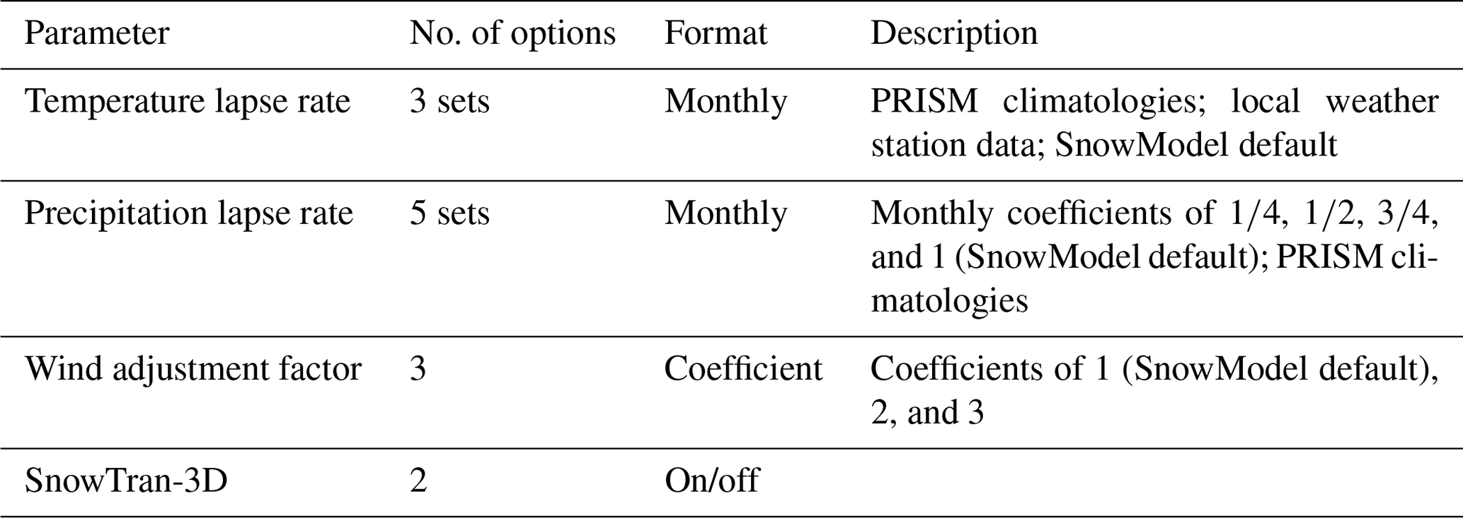
Table B1Top-performing parameter configurations from the calibration simulations.
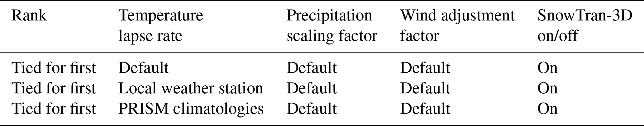
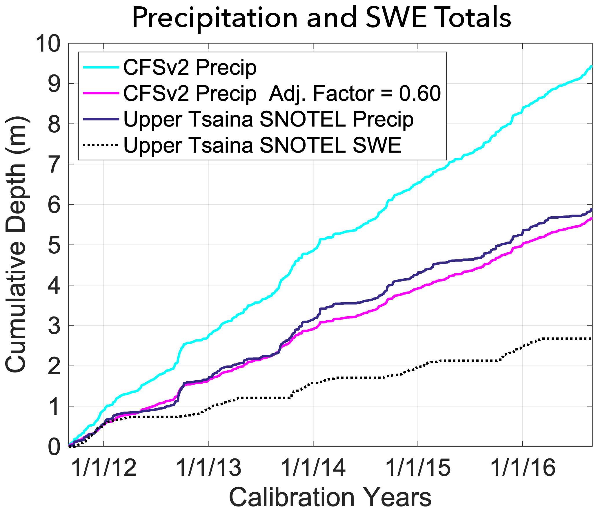
Figure C1Precipitation totals at the Upper Tsaina SNOTEL station compared to the CFSv2-forced model totals and the CFSv2-forced model totals with a precipitation adjustment factor. This overestimation of precipitation by the reanalysis product is a major factor in the quality of the calibration results.
Table D1Precipitation adjustment factor results. The best precipitation adjustment factors are shown, along with the root mean squared error (RMSE), the Nash–Sutcliffe efficiency (NSE), the Kling–Gupta efficiency (KGE), and the mean bias error (bias).
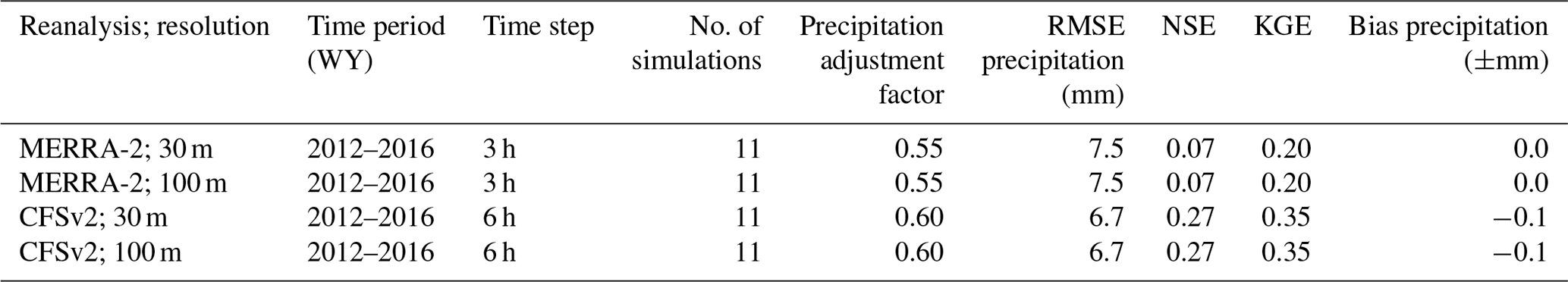
Table E1Ranked temporal results. Ensemble results from ranked by Kling–Gupta efficiency (KGE) score for water year (WY) 2017 (a) and WY2018 (b). Also included are the Nash–Sutcliffe efficiency (NSE) and the mean bias error (bias) values.

Table F1Ranked spatial results. Spatial distribution ensemble results ranked by Kolmogorov–Smirnov (KS) score for water year (WY) 2017 (a) and WY2018 (b). Also included are the root mean squared error (RMSE) and the median values.
The data sets used in this study can be found at the following locations.
-
Community Snow Observations website and snow depth data can be downloaded from http://app.communitysnowobs.org/ (Community Snow Observations Data Portal, 2021).
-
The snow depth to snow water equivalence calculator (Hill et al., 2019) can be found at https://doi.org/10.5281/zenodo.5225097 (Hill and Aragon, 2021).
-
Snow Telemetry data for the Upper Tsaina River station near Valdez, Alaska, are available from the Natural Resources Conservation Service website at https://wcc.sc.egov.usda.gov/nwcc/site?sitenum=1055 (Natural Resources Conservation Service, 2021).
-
Climate Forecast System version 2 (CFSv2) data (see Saha et al., 2011).
-
The CFSv2 data were accessed using Google Earth Engine, and a JavaScript version of the code used to download the data can be found at https://doi.org/10.5281/zenodo.5188622 (Crumley and Hill, 2021). A JavaScript version of the Google Earth Engine code written for this project is available at https://github.com/snowmodel-tools/preprocess_javascript (last access: 30 April 2020).
-
To convert the CFSv2 data downloaded from the Google Earth Engine to the necessary input file for MicroMet, we wrote the following MATLAB script: https://doi.org/10.5281/zenodo.5224852 (Hill et al., 2021).
-
The MERRA-2 weather reanalysis product from NASA's Global Modeling and Assimilation office (see Gelaro et al., 2017).
-
The National Elevation Dataset (see Gesch et al., 2002).
-
The National Land Cover Database 2011 data set (see Homer et al., 2015).
RLC, DFH, GJW, KWJ, and AAA designed the research questions and decided on the methods. RLC, GJW, KWJ, CC, and DFH conducted the fieldwork in the study area, including snowpack sampling and remote sensing surveys. RLC and DFH oversaw the analysis of the paper. AAA designed and maintained the CSO website and snow data set, with contributions from all authors. Community Snow Observations participants and all authors contributed snow depth measurements. RLC prepared the paper, with contributions from all authors during editing and review process.
The authors declare that they have no conflict of interest.
Publisher’s note: Copernicus Publications remains neutral with regard to jurisdictional claims in published maps and institutional affiliations.
We thank the participants in the Community Snow Observations for their submissions, Glen Liston, for providing the model code and occasional guidance, and the Los Alamos National Laboratory, which approved the dissemination of this paper with the assigned number of LA-UR-21-26394.
This research has been supported by NASA (grant no. NNX17AG67A) and the Consortium of Universities for the Advancement of Hydrologic Science, Inc. (CUAHSI; Pathfinder Fellowship grant). Anthony A. Arendt was partially supported by the Washington Research Foundation and by a Data Science Environments project award to the University of Washington eScience Institute from the Gordon and Betty Moore and the Alfred P. Sloan Foundations.
This paper was edited by Jan Seibert and reviewed by four anonymous referees.
Anderton, S. P., White, S. M., and Alvera, B.: Evaluation of spatial variability in snow water equivalent for a high mountain catchment, Hydrol. Process., 18, 435–453, https://doi.org/10.1002/hyp.1319, 2004.
Baba, M., Gascoin, S., Jarlan, L., Simonneaux, V., and Hanich, L.: Variations of the Snow Water Equivalent in the Ourika Catchment (Morocco) over 2000–2018 Using Downscaled MERRA-2 Data, Water, 1, 1120, https://doi.org/10.3390/w10091120, 2018.
Bales, R. C., Molotch, N. P., Painter, T. H., Dettinger, M. D., Rice, R., and Dozier, J.: Mountain hydrology of the western United States, Water Resour. Res., 42, W08432, https://doi.org/10.1029/2005WR004387, 2006.
Barnes, S. L.: A technique for maximizing details in numerical weather map analysis, J. Appl. Meteorol., 3, 396–409, https://doi.org/10.1175/1520-0450(1964)003<0396:ATFMDI>2.0.CO;2, 1964.
Barnes, S. L.: Mesoscale objective map analysis using weighted time-series observations, Technical Report, National Severe Storms Lab., Norman, Oklahoma, 1973.
Barnett, T. P., Adam, J. C., and Lettenmaier, D. P.: Potential impacts of a warming climate on water availability in snow-dominated regions, Nature, 438, 303, https://doi.org/10.1038/nature04141, 2005.
Beamer, J. P., Hill, D. F., Arendt, A., and Liston, G. E.: High-resolution modeling of coastal freshwater discharge and glacier mass balance in the Gulf of Alaska watershed, Water Resour. Res., 52, 3888–3909, https://doi.org/10.1002/2015WR018457, 2016.
Beamer, J. P., Hill, D. F., McGrath, D., Arendt, A., and Kienholz, C.: Hydrologic impacts of changes in climate and glacier extent in the Gulf of Alaska watershed, Water Resour. Res., 53, 7502–7520, https://doi.org/10.1002/2016WR020033, 2017.
Blöschl, G.: Scaling issues in snow hydrology, Hydrol. Process., 13, 2149–2175, https://doi.org/10.1002/(SICI)1099-1085(199910)13:14/15<2149::AID-HYP847>3.0.CO;2-8, 1999.
Blöschl, G. and Kirnbauer, R.: An analysis of snow cover patterns in a small alpine catchment, Hydrol. Process., 6, 99–109, https://doi.org/10.1002/hyp.3360060109, 1992.
Bohr, G. S. and Aguado, E.: Use of April 1 SWE measurements as estimates of peak seasonal snowpack and total cold-season precipitation, Water Resour. Res., 37, 51–60, https://doi.org/10.1029/2000WR900256, 2001.
Bonney, R., Cooper, C. B., Dickinson, J., Kelling, S., Phillips, T., Rosenberg, K. V., and Shirk, J.: Citizen science: a developing tool for expanding science knowledge and scientific literacy, BioScience, 59, 977–984, https://doi.org/10.1525/bio.2009.59.11.9, 2009.
Bühler, Y., Adams, M. S., Bösch, R., and Stoffel, A.: Mapping snow depth in alpine terrain with unmanned aerial systems (UASs): potential and limitations, The Cryosphere, 10, 1075–1088, https://doi.org/10.5194/tc-10-1075-2016, 2016.
Buytaert, W., Zulkafli, Z., Grainger, S., Acosta, L., Alemie, T. C., Bastiaensen, J., De Bièvre, B., Bhusal, J., Clark, J., Dewulf, A., and Foggin, M.: Citizen science in hydrology and water resources: opportunities for knowledge generation, ecosystem service management, and sustainable development, Front. Earth Sci., 2, 26, https://doi.org/10.3389/feart.2014.00026, 2014.
Carrassi, A., Bocquet, M., Bertino, L., and Evensen, G.: Data assimilation in the geosciences: An overview of methods, issues, and perspectives, WIRES Clim. Change, 9, e535, https://doi.org/10.1002/wcc.535, 2018.
Carroll, T., Cline, D., Fall, G., Nilsson, A., Li, L., and Rost, A.: NOHRSC operations and the simulation of snow cover properties for the coterminous US, in: Proc. 69th Annual Meeting of the Western Snow Conf., Sun Valley Idaho, 1–14, 2001.
Carter, S., Carter, P., and Levison, J.: Skier triggered surface hoar: A discussion of avalanche involvements during the 2006 Valdez Chugach helicopter ski season, in: Proceedings of International Snow Science Workshop, 860–867, 2006.
Clark, M. P., Slater, A. G., Barrett, A. P., Hay, L. E., McCabe, G. J., Rajagopalan, B., and Leavesley, G. H.: Assimilation of snow covered area information into hydrologic and land-surface models, Adv. Water Resour., 29, 1209–1221, https://doi.org/10.1016/j.advwatres.2005.10.001, 2006.
Clark, M. P., Hendrikx, J., Slater, A. G., Kavetski, D., Anderson, B., Cullen, N. J., Kerr, T., Örn Hreinsson, E., and Woods, R. A.: Representing spatial variability of snow water equivalent in hydrologic and land-surface models: A review, Water Resour. Res., 47, W07539, https://doi.org/10.1029/2011WR010745, 2011.
Community Snow Observations Data Portal: http://app.communitysnowobs.org/, last access: 20 August 2021.
Contosta, A. R., Adolph, A., Burchsted, D., Burakowski, E., Green, M., Guerra, D., Albert, M., Dibb, J., Martin, M., McDowell, W. H., and Routhier, M.: A longer vernal window: the role of winter coldness and snowpack in driving spring transitions and lags, Glob. Change Biol., 23, 1610–1625, https://doi.org/10.1111/gcb.13517, 2017.
Cooper, C. B., Dickinson J., Phillips, T., and Bonney, R.: Citizen science as a tool for conservation in residential ecosystems, Ecol. Soc., 12, 11, http://www.ecologyandsociety.org/vol12/iss2/art11/ (last access: 5 May 2020), 2007.
Cosgrove, C. L., Wells, J., Nolin, A. W., Putera, J., and Prugh, L. R.: Seasonal influence of snow conditions on Dall's sheep productivity in Wrangell-St Elias National Park and Preserve, PloS One, 16, e0244787, https://doi.org/10.1371/journal.pone.0244787, 2021.
Crumley, R. and Hill D.; Preprocessing model inputs from Google Earth Engine tool, Zenodo [code], https://doi.org/10.5281/zenodo.5188622, 2021.
Crumley, R. L., Hill, D. F., Beamer, J. P., and Holzenthal, E. R.: Seasonal components of freshwater runoff in Glacier Bay, Alaska: diverse spatial patterns and temporal change, The Cryosphere, 13, 1597–1619, https://doi.org/10.5194/tc-13-1597-2019, 2019.
Deems, J. S. and Painter, T. H.: Lidar measurement of snow depth: accuracy and error sources, in: Proceedings of the 2006 International Snow Science Workshop: Telluride, Colorado, USA, International Snow Science Workshop, 330–338, 2006.
Dickinson, J. L., Zuckerberg, B., and Bonter, D. N.: Citizen science as an ecological research tool: challenges and benefits, Annu. Rev. Ecol. Evol. S., 41, 149–172, https://doi.org/10.1146/annurev-ecolsys-102209-144636, 2010.
Dixon, D. and Boon, S.: Comparison of the SnowHydro snow sampler with existing snow tube designs, Hydrol. Process., 26, 2555–2562, https://doi.org/10.1002/hyp.9317, 2012.
Dressler, K. A., Fassnacht, S. R., and Bales, R. C.: A comparison of snow telemetry and snow course measurements in the Colorado River basin, J. Hydrometeorol., 7, 705–712, https://doi.org/10.1175/JHM506.1, 2006.
Elder, K., Rosenthal, W., and Davis, R. E.: Estimating the spatial distribution of snow water equivalence in a montane watershed, Hydrol. Process., 12, 1793–1808, https://doi.org/10.1002/(SICI)1099-1085(199808/09)12:10/11<1793::AID-HYP695>3.0.CO;2-K, 1998.
Fayad, A., Gascoin, S., Faour, G., López-Moreno, J. I., Drapeau, L., Le Page, M., and Escadafal, R.: Snow hydrology in Mediterranean mountain regions: A review, J. Hydrol., 551, 374–396, https://doi.org/10.1016/j.jhydrol.2017.05.063, 2017.
Fienen, M. N. and Lowry, C. S.: Social. Water – A crowdsourcing tool for environmental data acquisition, Comput. Geosci., 49, 164–169, https://doi.org/10.1016/j.cageo.2012.06.015, 2012.
Fletcher, S. J., Liston, G. E., Hiemstra, C. A., and Miller, S. D.: Assimilating MODIS and AMSR-E snow observations in a snow evolution model, J. Hydrometeorol., 13, 1475–1492, https://doi.org/10.1175/JHM-D-11-082.1, 2012.
Garnett, R. and Stewart, R.: Comparison of GPS units and mobile Apple GPS capabilities in an urban landscape, Cartogr. Geogr. Inform., 42, 1–8, https://doi.org/10.1080/15230406.2014.974074, 2015.
Gelaro, R., McCarty, W., Suárez, M. J., Todling, R., Molod, A., Takacs, L., Randles, C. A., Darmenov, A., Bosilovich, M. G., Reichle, R., and Wargan, K.: The modern-era retrospective analysis for research and applications, version 2 (MERRA-2), J. Climate, 30, 5419–5454, https://doi.org/10.1175/JCLI-D-16-0758.1, 2017.
Gesch, D., Oimoen, M., Greenlee, S., Nelson, C., Steuck, M., and Tyler, D.: The national elevation dataset, Photogramm. Eng. Rem. S., 68, 5–32, 2002.
Haberkorn, A.: European Snow Booklet – an Inventory of Snow Measurements in Europe, EnviDat, https://doi.org/10.16904/envidat.59, 2019.
Hall, D. K. and Riggs, G. A., and Salomonson V. V.: MODIS/Terra Snow Cover Daily L3 Global 500 m Grid, Version 6. Boulder, CO, NASA National Snow and Ice Data Center Distributed Active Archive Center [data set], https://doi.org/10.5067/MODIS/MOD10A1.006, 2016.
Han, E., Merwade, V., and Heathman, G. C.: Implementation of surface soil moisture data assimilation with watershed scale distributed hydrological model, J. Hydrol., 416, 98–117, https://doi.org/10.1016/j.jhydrol.2011.11.039, 2012.
Hedrick, A. R., Marks, D., Havens, S., Robertson, M., Johnson, M., Sandusky, M., Marshall, H. P., Kormos, P. R., Bormann, K. J., and Painter, T. H.: Direct insertion of NASA Airborne Snow Observatory-derived snow depth time series into the iSnobal energy balance snow model, Water Resour. Res., 54, 8045–8063, https://doi.org/10.1029/2018WR023190, 2018.
Helmert, J., Lange, M., Dong, J., De Rosnay, P., Gustafsson, D., Churulin, E., Kurzeneva, E., Müller, R., Trentmann, J., Souverijns, N., and Koch, R.: 1st Snow Data Assimilation Workshop in the framework of COST HarmoSnow ESSEM 1404, Meteorol. Z., 27, 325–333, https://doi.org/10.1127/metz/2018/0906, 2018.
Hendrikx, J., Johnson, J., and Shelly, C.: Using GPS tracking to explore terrain preferences of heli-ski guides, Journal of outdoor recreation and tourism, 13, 34–43, https://doi.org/10.1016/j.jort.2015.11.004, 2016.
Hill, D. and Aragon, C.: Snow density calculator, Zenodo [code], https://doi.org/10.5281/zenodo.5225097, 2021.
Hill, D., Wolken, G., Wikstrom Jones K., Crumley, R., and Arendt, A.: Crowdsourcing snow depth data with citizen scientists, Eos, 99, https://doi.org/10.1029/2018EO108991, 2018.
Hill, D., Aragon, C., and Crumley, R.: Preprocessing Micromet inputs from Google Earth Engine, Zenodo [code], https://doi.org/10.5281/zenodo.5224852, 2021.
Hill, D. F., Burakowski, E. A., Crumley, R. L., Keon, J., Hu, J. M., Arendt, A. A., Wikstrom Jones, K., and Wolken, G. J.: Converting snow depth to snow water equivalent using climatological variables, The Cryosphere, 13, 1767–1784, https://doi.org/10.5194/tc-13-1767-2019, 2019.
Holko, L., Gorbachova, L., and Kostka, Z.: Snow hydrology in central Europe, Geography Compass, 5, 200–218, https://doi.org/10.1111/j.1749-8198.2011.00412.x, 2011.
Homer, C., Dewitz, J., Yang, L., Jin, S., Danielson, P., Xian, G., Coulston, J., Herold, N., Wickham, J., and Megown, K.: Completion of the 2011 National Land Cover Database for the conterminous United States–representing a decade of land cover change information. Photogrammetric Engineering & Remote Sensing, 81, 345–354, 2015.
Jonas, T., Marty, C., and Magnusson, J.: Estimating the snow water equivalent from snow depth measurements in the Swiss Alps, J. Hydrology, 378, 161–167, https://doi.org/10.1016/j.jhydrol.2009.09.021, 2009.
Johnson, J. B.: A theory of pressure sensor performance in snow, Hydrol. Process., 18, 53–64, https://doi.org/10.1002/hyp.1310, 2003.
Johnson, J. B. and Schaefer, G. L.: The influence of thermal, hydrologic, and snow deformation mechanisms on snow water equivalent pressure sensor accuracy, Hydrol. Process., 16, 3529–3542, https://doi.org/10.1002/hyp.1236, 2002.
Kalnay, E.: Atmospheric modeling, data assimilation and predictability, Cambridge University Press, Cambridge, United Kingdom, 2003.
Kalnay, E., Kanamitsu, M., Kistler, R., Collins, W., Deaven, D., Gandin, L., Iredell, M., Saha, S., White, G., Woollen, J., and Zhu, Y.: The NCEP/NCAR 40-year reanalysis project, B. Am. Meteorol. Soc., 77, 437–471, https://doi.org/10.1175/1520-0477(1996)077<0437:TNYRP>2.0.CO;2, 1996.
Kapnick, S. and Hall, A.: Causes of recent changes in western North American snowpack, Clim. Dynam., 38, 1885–1899, https://doi.org/10.1007/s00382-011-1089-y, 2012.
King, J. M., Cabrera, A. R., and Kelly, R. E.: The Snowtweets Project: Communicating snow depth measurements from specialists and non-specialists via mobile communication technologies and social networks, AGU Fall Meeting Abstracts, Bibcode: 2009AGUFMED11A0562K, 2009.
Lader, R., Bhatt, U. S., Walsh, J. E., Rupp, T. S., and Bieniek, P. A.: Two-meter temperature and precipitation from atmospheric reanalysis evaluated for Alaska, J. Appl. Meteorol. Clim., 55, 901–922, https://doi.org/10.1175/JAMC-D-15-0162.1, 2016.
Lehning, M., Bartelt, P., Brown, B., Russi, T., Stöckli, U., and Zimmerli, M.: SNOWPACK model calculations for avalanche warning based upon a new network of weather and snow stations, Cold Reg. Sci. Technol., 30, 145–157, https://doi.org/10.1016/S0165-232X(99)00022-1, 1999.
Lehning, M., Völksch, I., Gustafsson, D., Nguyen, T. A., Stähli, M., and Zappa, M.: ALPINE3D: a detailed model of mountain surface processes and its application to snow hydrology, Hydrol. Process., 20, 2111–2128, https://doi.org/10.1002/hyp.6204, 2006.
Li, D., Wigmore, O., Durand, M. T., Vander-Jagt, B., Margulis, S. A., Molotch, N. P., and Bales, R. C.: Potential of Balloon Photogrammetry for Spatially Continuous Snow Depth Measurements, IEEE Geosci. Remote S., 17, 1667–1671, https://doi.org/10.1109/LGRS.2019.2953481, 2019.
Liston, G. E. and Elder, K.: A distributed snow-evolution modeling system (SnowModel), J. Hydrometeorol., 7, 1259–1276, https://doi.org/10.1175/JHM548.1, 2006a.
Liston, G. E. and Elder, K.: A meteorological distribution system for high-resolution terrestrial modeling (MicroMet), J. Hydrometeorol., 7, 217–234, https://doi.org/10.1175/JHM486.1, 2006b.
Liston, G. E. and Hiemstra, C. A.: A simple data assimilation system for complex snow distributions (SnowAssim), J. Hydrometeorol., 9, 989–1004, https://doi.org/10.1175/2008JHM871.1, 2008.
Liston, G. E. and Hiemstra, C. A.: The changing cryosphere: Pan-Arctic snow trends (1979–2009), J. Climate, 24, 5691–5712, https://doi.org/10.1175/JCLI-D-11-00081.1, 2011.
Liston, G. E., Haehnel, R. B., Sturm, M., Hiemstra, C. A., Berezovskaya, S., and Tabler, R. D.: Simulating complex snow distributions in windy environments using SnowTran-3D, J. Glaciol., 53, 241–256, https://doi.org/10.3189/172756507782202865, 2007.
López-Moreno, J. I., Fassnacht, S. R., Heath, J. T., Musselman, K. N., Revuelto, J., Latron, J., Morán-Tejeda, E., and Jonas, T.: Small scale spatial variability of snow density and depth over complex alpine terrain: Implications for estimating snow water equivalent, Adv. Water Resour., 55, 40–52, https://doi.org/10.1016/j.advwatres.2012.08.010, 2013.
Lowry, C. S. and Fienen, M. N.: CrowdHydrology: crowdsourcing hydrologic data and engaging citizen scientists, GroundWater, 51, 151–156, https://doi.org/10.1111/j.1745-6584.2012.00956.x, 2013.
Luce, C. H., Tarboton, D. G., and Cooley, K. R.: The influence of the spatial distribution of snow on basin-averaged snowmelt, Hydrol. Process., 12, 1671–1683, https://doi.org/10.1002/(SICI)1099-1085(199808/09)12:10/11<1671::AID-HYP688>3.0.CO;2-N, 1998.
Luojus, K., Pulliainen, J., Takala, M., Derksen, C., Rott, H., Nagler, T., Solberg, R., Wiesmann, A., Metsamaki, S., Malnes, E., and Bojkov, B.: Investigating the feasibility of the GlobSnow snow water equivalent data for climate research purposes, in: 2010 IEEE International Geoscience and Remote Sensing Symposium, 4851–4853, https://doi.org/10.1109/IGARSS.2010.5741987, 2010.
Magnusson, J., Gustafsson, D., Hüsler, F., and Jonas, T.: Assimilation of point SWE data into a distributed snow cover model comparing two contrasting methods, Water Resour. Res., 50, 7816–7835, https://doi.org/10.1002/2014WR015302, 2014.
Magnusson, J., Winstral, A., Stordal, A. S., Essery, R., and Jonas, T.: Improving physically based snow simulations by assimilating snow depths using the particle filter, Water Resour. Res., 53, 1125–1143, https://doi.org/10.1002/2016WR019092, 2017.
Malik, M. J., van der Velde, R., Vekerdy, Z., and Su, Z. Assimilation of satellite-observed snow albedo in a land surface model, J. Hydrometeorol., 13, 1119–1130, https://doi.org/10.1175/JHM-D-11-0125.1, 2012.
Mankin, J. S., Viviroli, D., Singh, D., Hoekstra, A. Y., and Diffenbaugh, N. S.: The potential for snow to supply human water demand in the present and future, Environ. Res. Lett., 10, 114016, https://doi.org/10.1088/1748-9326/10/11/114016, 2015.
Margulis, S. A., Girotto, M., Cortés, G., and Durand, M.: A particle batch smoother approach to snow water equivalent estimation, J. Hydrometeorol., 16, 1752–1772, https://doi.org/10.1175/JHM-D-14-0177.1, 2015.
Marks, D., Domingo, J., Susong, D., Link, T., and Garen, D.: A spatially distributed energy balance snowmelt model for application in mountain basins, Hydrol. Process., 13, 1935–1959, https://doi.org/10.1002/(SICI)1099-1085(199909)13:12/13<1935::AID-HYP868>3.0.CO;2-C, 1999.
Massey, Jr., F. J.: The Kolmogorov-Smirnov test for goodness of fit, J. Am. Stat. Assoc., 46, 68–78, 1951.
McCreight, J. L., Small, E. E., and Larson, K. M.: Snow depth, density, and SWE estimates derived from GPS reflection data: Validation in the western US, Water Resour. Res., 50, 6892–6909, https://doi.org/10.1002/2014WR015561, 2014.
McGuire, M., Wood, A. W., Hamlet, A. F., and Lettenmaier, D. P.: Use of satellite data for streamflow and reservoir storage forecasts in the Snake River Basin, J. Water Resour. Plan. Man., 132, 97–110, https://doi.org/10.1061/(ASCE)0733-9496(2006)132:2(97), 2006.
McKinley, D. C., Miller-Rushing, A. J., Ballard, H. L., Bonney, R., Brown, H., Cook-Patton, S. C., Evans, D. M., French, R. A., Parrish, J. K., Phillips, T. B., and Ryan, S. F.: Citizen science can improve conservation science, natural resource management, and environmental protection, Biol. Conserv., 208, 15–28, https://doi.org/10.1016/j.biocon.2016.05.015, 2017.
McLaughlin, D.: An integrated approach to hydrologic data assimilation: interpolation, smoothing, and filtering, Adv. Water Resour., 25, 1275–1286, https://doi.org/10.1016/S0309-1708(02)00055-6, 2002.
McMillan, H. K., Hreinsson, E. Ö., Clark, M. P., Singh, S. K., Zammit, C., and Uddstrom, M. J.: Operational hydrological data assimilation with the recursive ensemble Kalman filter, Hydrol. Earth Syst. Sci., 17, 21–38, https://doi.org/10.5194/hess-17-21-2013, 2013.
Mernild, S. H., Liston, G. E., Hasholt, B., and Knudsen, N.T.: Snow distribution and melt modeling for Mittivakkat Glacier, Ammassalik Island, southeast Greenland, J. Hydrometeorol., 7, 808–824, https://doi.org/10.1175/JHM522.1, 2006.
Mernild, S. H., Liston, G. E., Hiemstra, C. A., Malmros, J. K., Yde, J. C., and McPhee, J.: The Andes Cordillera. Part I: snow distribution, properties, and trends (1979–2014), Int. J. Climatol., 37, 1680–1698, https://doi.org/10.1002/joc.4804, 2017a.
Mernild, S. H., Liston, G. E., Hiemstra, C. A., Yde, J. C., McPhee, J., and Malmros, J.K.: The Andes Cordillera. Part II: Rio Olivares Basin snow conditions (1979–2014), central Chile, Int. J. Climatol., 37, 1699–1715, https://doi.org/10.1002/joc.4828, 2017b.
Mesinger, F., DiMego, G., Kalnay, E., Mitchell, K., Shafran, P. C., Ebisuzaki, W., Jović, D., Woollen, J., Rogers, E., Berbery, E. H., and Ek, M. B.: North American regional reanalysis, B. Am. Meteorol. Soc., 87, 343–360, https://doi.org/10.1175/BAMS-87-3-343, 2006.
Molotch, N. P. and Bales, R. C.: Scaling snow observations from the point to the grid element: Implications for observation network design, Water Resour. Res., 41, W11421, https://doi.org/10.1029/2005WR004229, 2005.
Molotch, N. P., Colee, M. T., Bales, R. C., and Dozier, J.: Estimating the spatial distribution of snow water equivalent in an alpine basin using binary regression tree models: the impact of digital elevation data and independent variable selection, Hydrol. Process., 19, 1459–1479, https://doi.org/10.1002/hyp.5586, 2005.
Mote, P. W., Li, S., Lettenmaier, D. P., Xiao, M., and Engel, R.: Dramatic declines in snowpack in the western US, Npj Climate and Atmospheric Science, 1, 1–6, https://doi.org/10.1038/s41612-018-0012-1, 2018.
NOHRSC: Snow Data Assimilation System (SNODAS) Data Products at NSIDC, Version 1, Boulder, Colorado USA. NSIDC: National Snow and Ice Data Center, https://doi.org/10.7265/N5TB14TC, 2004.
Pagano, T., Garen, D., Perkins, T., and Pasteris, P.: Daily updating of operational statistical seasonal water supply forecasts for the western U.S., J. Am. Water Resour. As., 45, 767–778, https://doi.org/10.1111/j.1752-1688.2009.00321.x, 2009.
Painter, T. H., Berisford, D. F., Boardman, J. W., Bormann, K. J., Deems, J. S., Gehrke, F., Hedrick, A., Joyce, M., Laidlaw, R., Marks, D., and Mattmann, C.: The Airborne Snow Observatory: Fusion of scanning lidar, imaging spectrometer, and physically-based modeling for mapping snow water equivalent and snow albedo, Remote Sens. Environ., 184, 139–152, https://doi.org/10.1016/j.rse.2016.06.018, 2016.
Park, S. K. and Xu, L. (Eds.): Data assimilation for atmospheric, oceanic and hydrologic applications, Vol. 2, Springer Science & Business Media, Heidelberg, Germany, 2013.
Pistocchi, A.: Simple estimation of snow density in an Alpine region, J. Hydrol.: Regional Studies, 6, 82–89, https://doi.org/10.1016/j.ejrh.2016.03.004, 2016.
Pomeroy, J. W., Gray, D. M., and Landine, P. G. The prairie blowing snow model: characteristics, validation, operation, J. Hydrol., 144, 165–192, https://doi.org/10.1016/0022-1694(93)90171-5, 1993.
Rabier, F.: Overview of global data assimilation developments in numerical weather-prediction centres, Q. J. Roy. Meteor. Soc., 131, 3215–3233, https://doi.org/10.1256/qj.05.129, 2005.
Reges, H. W., Doesken, N., Turner, J., Newman, N., Bergantino, A., and Schwalbe, Z.: COCORAHS: The evolution and accomplishments of a volunteer rain gauge network, B. Am. Meteorol. Soc., 97, 1831–1846, https://doi.org/10.1175/BAMS-D-14-00213.1, 2016.
Reichle, R. H.: Data assimilation methods in the Earth sciences, Adv. Water Resour., 31, 1411–1418, https://doi.org/10.1016/j.advwatres.2008.01.001, 2008.
Reichle, R. H., McLaughlin, D. B., and Entekhabi, D.: Hydrologic data assimilation with the ensemble Kalman filter, Mon. Weather Rev., 130, 103–114, https://doi.org/10.1175/1520-0493(2002)130<0103:HDAWTE>2.0.CO;2, 2002.
Rice, R. and Bales, R. C.: Embedded-sensor network design for snow cover measurements around snow pillow and snow course sites in the Sierra Nevada of California, Water Resour. Res., 46, W03537, https://doi.org/10.1029/2008WR007318, 2010.
Riemann, R., Wilson, B. T., Lister, A., and Parks, S.: An effective assessment protocol for continuous geospatial datasets of forest characteristics using USFS Forest Inventory and Analysis (FIA) data, Remote Sens. Environ., 114, 2337–2352, https://doi.org/10.1016/j.rse.2010.05.010, 2010.
Rivington, M., Matthews, K. B., Bellocchi, G., and Buchan, K.: Evaluating uncertainty introduced to process-based simulation model estimates by alternative sources of meteorological data, Agr. Syst., 88, 451–471, https://doi.org/10.1016/j.agsy.2005.07.004, 2006.
Saha, S., Moorthi, S., Pan, H. L., Wu, X., Wang, J., Nadiga, S., Tripp, P., Kistler, R., Woollen, J., Behringer, D., and Liu, H.: The NCEP climate forecast system reanalysis, B. Am. Meteorol. Soc., 91, 1015–1058, https://doi.org/10.1175/2010BAMS3001.1, 2010.
Saha, S., Moorthi, S., Wu, X., Wang, J., Nadiga, S., Tripp, P., Behringer, D., Hou, Y., Chuang, H., Iredell, M., Ek, M., Meng, J., Yang, R., Mendez, M. P., van den Dool, H., Zhang, Q., Wang, W., Chen, M., and Becker, E.: NCEP Climate Forecast System Version 2 (CFSv2) 6-hourly Products. Research Data Archive at the National Center for Atmospheric Research, Computational and Information Systems Laboratory, Research Data Archive [data set], https://doi.org/10.5065/D61C1TXF, 2011.
Saha, S., Moorthi, S., Wu, X., Wang, J., Nadiga, S., Tripp, P., Behringer, D., Hou, Y. T., Chuang, H. Y., Iredell, M., and Ek, M.: The NCEP climate forecast system version 2, J. Climate, 27, 2185–2208, https://doi.org/10.1175/JCLI-D-12-00823.1, 2014.
Schmucki, E., Marty, C., Fierz, C., and Lehning, M.: Evaluation of modelled snow depth and snow water equivalent at three contrasting sites in Switzerland using SNOWPACK simulations driven by different meteorological data input, Cold Reg. Sci. Technol., 99, 27–37, https://doi.org/10.1016/j.coldregions.2013.12.004, 2014.
Schaefer, M. and Woodyer, T.: Assessing absolute and relative accuracy of recreation-grade and mobile phone GNSS devices: a method for informing device choice, Area, 47, 185–196, https://doi.org/10.1111/area.12172, 2015.
Schlögl, S., Marty, C., Bavay, M., and Lehning, M.: Sensitivity of Alpine3D modeled snow cover to modifications in DEM resolution, station coverage and meteorological input quantities, Environ. Modell. Softw., 83, 387–396, https://doi.org/10.1016/j.envsoft.2016.02.017, 2016.
Schneider, C., Laizé, C. L. R., Acreman, M. C., and Flörke, M.: How will climate change modify river flow regimes in Europe?, Hydrol. Earth Syst. Sci., 17, 325–339, https://doi.org/10.5194/hess-17-325-2013, 2013.
Seibert, J., Strobl, B., Etter, S., Hummer, P., and van Meerveld, H.J.: Virtual staff gauges for crowd-based stream level observations, Front. Earth Sci., 7, 70, https://doi.org/10.3389/feart.2019.00070, 2019.
Serreze, M. C., Clark, M. P., Armstrong, R. L., McGinnis, D. A., and Pulwarty, R. S.: Characteristics of the western United States snowpack from snowpack telemetry (SNOTEL) data, Water Resour. Res., 35, 2145–2160, https://doi.org/10.1029/1999WR900090, 1999.
Shulski, M. and Wendler, G.: The climate of Alaska, University of Alaska Press, Fairbanks, Alaska, USA, 2007.
Silvertown, J.: A new dawn for citizen science, Trends Ecol. Evol., 24, 467–471, https://doi.org/10.1016/j.tree.2009.03.017, 2009.
Sturm, M.: White water: Fifty years of snow research in WRR and the outlook for the future, Water Resour. Res., 51, 4948–4965, https://doi.org/10.1002/2015WR017242, 2015.
Sturm, M. and Wagner, A. M.: Using repeated patterns in snow distribution modeling: An Arctic example, Water Resour. Res., 46, W12549, https://doi.org/10.1029/2010WR009434, 2010.
Sturm, M., Holmgren, J., and Liston, G. E.: A seasonal snow cover classification system for local to global applications, J. Climate, 8, 1261–1283, https://doi.org/10.1175/1520-0442(1995)008<1261:ASSCCS>2.0.CO;2, 1995.
Sturm, M., Taras, B., Liston, G., Derksen, C., Jonas, T., and Lea, J.: Estimating Snow Water Equivalent Using Snow Depth Data and Climate Classes, J. Hydrometeorol., 11, 1380–1394, https://doi.org/10.1175/2010JHM1202.1, 2010.
Trujillo, E., Molotch, N. P., Goulden, M. L., Kelly, A. E., and Bales, R. C.: Elevation-dependent influence of snow accumulation on forest greening, Nat. Geosci., 5, 705–709, https://doi.org/10.1038/ngeo1571, 2012.
Natural Resources Conservation Service, Upper Tsaina SNOTEL Station Data Porta: https://wcc.sc.egov.usda.gov/nwcc/site?sitenum=1055, last access: 20 August 2021.
van Meerveld, H. J. I., Vis, M. J. P., and Seibert, J.: Information content of stream level class data for hydrological model calibration, Hydrol. Earth Syst. Sci., 21, 4895–4905, https://doi.org/10.5194/hess-21-4895-2017, 2017.
Viviroli, D., Dürr, H. H., Messerli, B., Meybeck, M., and Weingartner, R.: Mountains of the world, water towers for humanity: Typology, mapping, and global significance, Water Resour. Res., 43, W07447, https://doi.org/10.1029/2006WR005653, 2007.
Wagner, W.: Investigating the snow climate of Turnagain Pass, Alaska, in: Proceedings of the International Snow Science Workshop, Anchorage, AK, 913–917, 2012.
Wiggins, A. and Crowston, K.: From conservation to crowdsourcing: A typology of citizen science, in: 2011 44th Hawaii international conference on system sciences, 1–10, https://doi.org/10.1109/HICSS.2011.207, 2011.
Wrzesien, M. L., Durand, M. T., Pavelsky, T. M., Howat, I. M., Margulis, S. A., and Huning, L. S.: Comparison of methods to estimate snow water equivalent at the mountain range scale: a case study of the California Sierra Nevada, J. Hydrometeorol., 18, 1101–1119, https://doi.org/10.1175/JHM-D-16-0246.1, 2017.
Yeeles, A.: Citizen snow-scientists trek into the back country, Nat. Clim. Change, 8, 944, https://doi.org/10.1038/s41558-018-0329-0, 2018.
Young, J. C., Pettit, E., Arendt, A., Hood, E., Liston, G. E., and Beamer, J.: A changing hydrological regime: Trends in magnitude and timing of glacier ice melt and glacier runoff in a high latitude coastal watershed, Water Resour. Res., 57, e2020WR027404, https://doi.org/10.1029/2020WR027404, 2020.
- Abstract
- Introduction
- Study area
- Methods and data sets
- Calibration
- Experimental design
- Results
- Discussion
- Conclusions
- Appendix A
- Appendix B
- Appendix C
- Appendix D
- Appendix E
- Appendix F
- Code and data availability
- Author contributions
- Competing interests
- Disclaimer
- Acknowledgements
- Financial support
- Review statement
- References