The accuracy of temporal upscaling of instantaneous evapotranspiration to daily values with seven upscaling methods

This study evaluated the accuracy of seven upscaling methods in simulating daily latent heat flux (LE) from instantaneous values using observations from 148 global sites under all sky conditions and at different times during the day. Daily atmospheric transmissivity (τ) was used to represent the sky conditions. The results showed that all seven methods could accurately simulate daily LE from instantaneous values. The mean and median of Nash–Sutcliffe efficiency were 0.80 and 0.85, respectively, and the corresponding determination coefficients were 0.87 and 0.90, respectively. The sine and Gaussian function methods simulated mean values with relatively higher accuracy, with relative errors generally within ±10 %. The evaporative fraction (EF) methods, which use potential evapotranspiration and incoming shortwave radiation, performed relatively better than the other methods in simulating daily series. Overall, the EF method using potential evapotranspiration had the highest accuracy. However, the sine function and the EF method using extraterrestrial solar irradiance are recommended in upscaling applications because of the relatively minimal data requirements of these methods and their comparable or relatively higher accuracy. The intra-day distribution of the LE showed greater consistency with the Gaussian function than the sine function. However, the accuracy of simulated daily LE series using the Gaussian function method did not improve significantly compared with the sine function method. The simulation accuracy showed a minor difference when using the same type of method, for example, the same type of mathematical function or EF method. In any upscaling scheme, the simulation accuracy from multi-time values was significantly higher than that from a single-time value. Therefore, when multi-time data are available, multi-time values should be used in evapotranspiration upscaling. The upscaling methods show the ability to accurately simulate daily LE from instantaneous values from 09:00 to 15:00, particularly for instantaneous values between 11:00 and 14:00. However, outside of this time range the upscaling methods performed poorly. These methods can simulate daily LE series with high accuracy at τ > 0.6; when τ < 0.6, simulation accuracy is significantly affected by sky conditions and is generally positively related to daily atmospheric transmissivity. Although every upscaling scheme can accurately simulate daily LE from instantaneous values at most sites, this ability is lost at tropical rainforest and tropical monsoon sites.

1 Introduction

Evapotranspiration (ET) is a critical and unique bridge connecting the hydrologic cycle, surface energy balance, and carbon cycle (Jasechko et al., 2013; Lian et al., 2018). Approximately 60 % of precipitation on the global land surface returns to the atmosphere via ET (Oki and Kanae, 2006). More than half of the solar energy absorbed by land surfaces is currently used in the process of ET (Trenberth et al., 2009). Accurate simulations of ET represent the core of hydrologic processes, crop growth, and ecosystem water efficiency simulations (Ponce-Campos et al., 2013). These simulations are important for agriculture, ecology, and water resource management. However, field ET observations are expensive and labor-intensive (Jaksa et al., 2013) and cannot meet the required level of spatial accuracy. In recent decades, remote sensing ET retrieval based on the combination of satellite remote sensing data and the land surface energy model has become an increasingly important area of research, as it can represent the spatial heterogeneity of terrestrial ET at regional or global scales (Jung et al., 2010; Miralles et al., 2011; Mu et al., 2011; Zhang et al., 2019).

However, the remote sensing technique can only detect the instantaneous ET rate at the time of satellite overpasses. Additionally, instantaneous ET data are not useable for practical applications such as ecohydrological modeling and water resource management. For practical purposes, we are concerned with ET over a period of time; temporal upscaling of instantaneous ET over a period of time is necessary for remote sensing ET maps. Temporal upscaling has become one of the key issues and future research directions in the context of ET estimation from remote sensing data (Kalma et al., 2008; Li et al., 2009; Liu et al., 2020). A critical temporal upscaling step is upscaling from instantaneous to daily ET values (Chen and Liu, 2020).

Temporal upscaling methods have been reviewed thoroughly by several studies (Kalma et al., 2008; Li et al., 2009; Chen and Liu, 2020) and may be divided into three categories: the sine function method, the constant evaporative fraction (EF) method, and the constant ratio between the actual ET and potential ET (PET). Jackson (1983) assumed that diurnal solar irradiance and ET may be described by a sine function and developed this function to calculate daily ET from instantaneous values. Sugita and Brutsaert (1991) found that the evaporative fraction (EF) usually varies little during the daytime; the EF was defined as the ratio of the latent heat flux (LE =ρλE, where ρ and λ are the density of water and the latent heat of vaporization, respectively) to the available energy flux (R_n-G) at the surface. It may be assumed that EF is constant during daylight hours in order to upscale instantaneous ET to daily values. Investigations on the environmental factors that contribute to EF variability showed that EF is almost independent of major forcing factors, including air temperature, wind velocity, and incoming solar radiation (Crago, 1996; Gentine et al., 2007). However, cloudy weather and proximity to surface discontinuities or fronts may cause significant EF variability. The diurnal shape of EF is dependent on atmospheric forcing and surface conditions (Gentine et al., 2007); the EF is generally constant in the morning and increases sharply in the afternoon (Lhomme and Elguero, 1999; Gentine et al., 2007; Delogu et al., 2012). Hoedjes et al. (2008) found that although the EF method could accurately simulate daily ET under dry conditions, it significantly underestimated daily ET in wet conditions. They incorporated a daily scaling factor into EF for wet conditions by parameterizing the diurnal shape of EF as a function of incoming solar radiation and relative humidity; this was found to improve the accuracy of the simulation (Hoedjes et al., 2008; Delogu et al., 2012).

In addition to R_n-G, Brutsaert and Sugita (1992) used field measurements to validate effective EF ratios with net radiation (R_n) and incoming shortwave radiation (R_s). All these EF scaling factor approaches require surface energy flux data. An alternative approach with lower data requirements (Ryu et al., 2012; Van Niel et al., 2012) assumes a constant EF ratio for the LE to extraterrestrial solar irradiance (R_e). Similarly to the sine function method, this temporal upscaling scheme requires only latitude, longitude, and time as data inputs. EF methods based on variables such as R_n-G, R_n, R_s, and R_e are abbreviated as EF(R_n-G), EF(R_n), EF(R_s), and EF(R_e), respectively. Another temporal upscaling approach is maintaining a constant ratio between the actual ET and the PET (Kalma et al., 2008). Allen et al. (2007) proposed a constant ETrF in which PET was calculated using the reference ET during the daytime for temporal upscaling. Tang and Li (2017a, b) developed a decoupling factor using the Priestley–Taylor equation for PET. This decoupling factor method provides a theoretical framework for temporal upscaling (Chen and Liu, 2020). However, the ETrF approach requires additional weather measurements including air temperature, humidity, atmospheric pressure, and wind speed that are only recorded when the satellite overpasses.

All these methods are only used for upscaling daytime ET; as such, upscaling methods may underestimate daily ET due to nocturnal transpiration, which is the main cause of uncertainty in ET upscaling (Kalma et al., 2008; Blatchford et al., 2019). There have been several evaluations of these upscaling methods, which have found that the accuracy of the upscaling methods varies between regions. Zhang and Lemeur (1995) evaluated the sine function and EF(R_n-G) using an experiment in southwestern France, finding that both methods could accurately estimate daily ET from instantaneous measurements; they recommended a sine function due to its lower data requirements. The sine function and three EF methods, R_n, R_n-G, and R_e, were evaluated for the upscaling of monthly ET at two sites in Australia (Van Niel et al., 2012). A monthly bias was used to correct the upscaling methods; the results showed that the EF(R_n) was the preferable monthly upscaling method, as it had the lowest root-mean-square deviation (RMSD) before and after correction. The evaluation of EF and ETrF methods at four sites in France and Morocco showed that the EF method outperforms the ETrF method at sites experiencing a higher frequency of water stress periods (Delogu et al., 2012). Cammalleri et al. (2014) evaluated four methods, EF(R_n-G), EF(R_s), EF(R_e), and ETrF, in upscaling daily ET at 12 AmeriFlux stations. They found that the EF(R_s) method showed more robust overall performance in terms of accuracy and site-to-site variability. In contrast, Tang et al. (2013) evaluated four upscaling methods (EF(R_n-G), EF(R_e), EF(R_s), and ETrF) for daily LE simulations at a flux site in China. Their results showed that the ETrF method had the best performance among the four methods, while the EF(R_s) method was the second best. In general, previous research has largely evaluated upscaling methods on a regional scale. Based on 126 FLUXNET global sites, Wandera et al. (2017) evaluated three EF methods – R_s, R_e, and R_n-G – finding that the EF(R_s) method yielded relatively better accuracy in daily ET simulations. However, they only used EF methods for global evaluation.

The FLUXNET dataset provides a good opportunity to evaluate upscaling methods at the global scale (Pastorello et al., 2020) and has been widely used to evaluate ET estimation from remote sensing data (Fisher et al., 2008; Ershadi et al., 2014; Carter and Liang, 2018; Knox et al., 2019; Pastorello et al., 2020). The new FLUXNET-CH4 community product was released in 2020; this data series has been expanded to 2018. In 2020, the FLUXNET dataset published the observation height and vegetation height of each site, enabling the calculation of PET using the Penman–Monteith equation. This calculation is more consistent with the actual observational land surface than the reference ET. This study uses the FLUXNET dataset to comprehensively evaluate the ability of various upscaling schemes to accurately simulate daily LE at global flux measurement sites.

This study addresses four key objectives: (1) evaluating the accuracy of seven upscaling methods (the sine function, EF, and ETrF methods) in simulating daily LE from instantaneous values; (2) investigating the performance of upscaling methods under all sky conditions and calibrating the optimal threshold of sky conditions required to accurately simulate daily LE; (3) evaluating the simulation accuracy of upscaling methods at different times during the day; (4) investigating the spatial distribution of simulation accuracy at global flux observation sites.

2 Materials and methods

2.1 Observation data

This study used the FLUXNET eddy covariance observations that cover all continents; this includes the FLUXNET2015 (Pastorello et al., 2020) and FLUXNET-CH4 community products (Knox et al., 2019). FLUXNET2015 contains 212 observation sites from 1991 to 2014, while the FLUXNET-CH4 community product contains 81 sites from 2006 to 2018. The longest observational record was 25 years, while the shortest record was less than 1 year. Half-hourly data series on LE, R_s, R_n, and ground heat flux (G) were used for the upscaling schemes, while the observed air temperature, wind speed, atmospheric pressure, vapor pressure deficit, crop heights, observation height of wind, and humidity data were used in the Penman–Monteith equation. All missing values were eliminated; for example, if there were missing values on a certain day, all data on that day were discarded. As such, only days with fully available half-hourly data were used in the analysis. Then, only sites with a data series longer than 360 d were used. These eliminations ultimately meant a total of 122 FLUXNET2015 sites and 42 FLUXNET-CH4 sites were used in the analysis due to the lack of observations (Table S1). There were 16 sites belonging to both FLUXNET2015 and FLUXNET-CH4, and flux observation data from four sites in Australia were obtained from the TERN OzFlux dataset; the latter dataset was a long and continuous series up to 2019 (Beringer et al., 2016). LE was corrected using the energy balance closure correction factor.

Figure 1 Location of eddy covariance observations.

2.2 Methods of temporal upscaling of instantaneous λET to daily values

A Gaussian function was used in this study in addition to the widely used sine function. The distribution of λET (LE) during the daytime was more in line with the Gaussian function (this is shown in Sect. 3.1). In total, seven temporal upscaling methods for upscaling instantaneous LE to daily values were evaluated; this includes the sine function, Gaussian function, four EFs – EF(R_n-G), EF(R_n), EF(R_s), and EF(R_e) – and the ETrF methods. In general, the relationship between instantaneous LE and LE over time may be expressed as follows:

$$\begin{array}{}\text{(1)}& {\mathrm{LE}}_T={\int }_{t=\mathrm{0}}^T{\mathrm{LE}}_t\mathrm{d}t,\end{array}$$

where LE_T and LE_t are the LE over a period of time and instantaneous LE, respectively.

The sine (Jackson, 1983) and Gaussian function upscaling methods assume that the daytime LE obeys the sine and Gaussian functions, respectively:

$$\begin{array}{}\text{(2)}& {\displaystyle }{\mathrm{SINE}}_t=\sin \left(\mathit{\pi }{\displaystyle \frac{t-t_{\mathrm{0}}}{t_n-t_{\mathrm{0}}}}\right),\text{(3)}& {\displaystyle }{\mathrm{GAUSSIAN}}_t={\displaystyle \frac{\mathrm{1}}{\mathit{\sigma }\sqrt{\mathrm{2}\mathit{\pi }}}}{e}^{-\frac{\mathrm{1}}{\mathrm{2}}(\frac{t-\mathit{\mu }}{\mathit{\sigma }}{)}^{\mathrm{2}}},\end{array}$$

where t₀ and t_n are the sunrise and sunset times, respectively; μ is the solar noon time, equal to (t₀+t_n)$/\mathrm{2}$; and σ is a shape parameter of the Gaussian function. Sunrise and sunset times were calculated using the National Oceanic and Atmospheric Administration (NOAA) solar calculations (https://www.esrl.noaa.gov/gmd/grad/solcalc/calcdetails.html, last access: 3 August 2021). Subsequently, the sine and Gaussian function upscaling methods may be described as follows:

$$\begin{array}{}\text{(4)}& {\displaystyle }{\mathrm{LE}}_{\mathrm{d}}={\displaystyle \frac{\frac{\mathrm{1}}{n}{\sum }_{t=t_{\mathrm{0}}}^{t_n}{\mathrm{SINE}}_t}{{\mathrm{SINE}}_t}}{\mathrm{LE}}_i,\text{(5)}& {\displaystyle }{\mathrm{LE}}_{\mathrm{d}}={\displaystyle \frac{\frac{\mathrm{1}}{n}{\sum }_{t=t_{\mathrm{0}}}^{t_n}{\mathrm{GAUSSIAN}}_t}{{\mathrm{GAUSSIAN}}_t}}{\mathrm{LE}}_i,\end{array}$$

where LE_d is the simulated daily LE during the daytime, and LE_i is the instantaneous LE used in the simulation. The LE_t was calculated using Eqs. (2) and (3) for the sine and Gaussian functions, respectively.

The EF and ETrF methods assume a constant ratio between LE and the upscaling variable; this may be described as follows:

$$\begin{array}{}\text{(6)}& {\displaystyle \frac{{\mathrm{LE}}_{\mathrm{d}}}{V_{\mathrm{d}}}}={\displaystyle \frac{{\mathrm{LE}}_{\mathrm{i}}}{V_{\mathrm{i}}}},\end{array}$$

where LE_i and LE_d are the instantaneous and daytime LE, respectively, and V_i and V_d are the instantaneous and daily upscaling variables, respectively.

The four EF methods involve the upscaling variables, R_n, R_n-G, R_s and R_e; the former three variables are measured by FLUXNET. R_e, which is also known as the top-of-atmosphere solar irradiance, is calculated by the following equation (Ryu et al., 2012):

$$\begin{array}{}\text{(7)}& R_{\mathrm{e}}=S_{\mathrm{sc}}\times [\mathrm{1}+\mathrm{0.033}\cos \left({\displaystyle \frac{\mathrm{2}\mathit{\pi }\mathrm{DOY}}{Y_{\mathrm{dmax}}}}\right)]\cos \mathit{\beta },\end{array}$$

where S_sc is the solar constant (1360 W m⁻²); DOY is the day of the year; Y_dmax is the maximum number of days (365 or 366) for the specified year; β is the specific time-of-day solar zenith angle calculated using the NOAA solar calculations.

The ETrF method involves the upscaling variable, PET, herein referred to as EF(PET); PET is calculated using the Penman–Monteith equation (Penman, 1948; Monteith, 1981; Allen et al., 1998):

$$\begin{array}{}\text{(8)}& \mathit{\rho }\mathit{\lambda }E={\displaystyle \frac{\mathrm{\Delta }\left(R_{\mathrm{n}}-G\right)+{\mathit{\rho }}_{\mathrm{a}}{c}_{\mathrm{p}}\frac{(e_{\mathrm{s}}-e_{\mathrm{a}})}{r_{\mathrm{a}}}}{\mathrm{\Delta }+\mathit{\gamma }\left(\mathrm{1}+\frac{r_{\mathrm{s}}}{r_{\mathrm{a}}}\right)}},\end{array}$$

where ρ is the density of water; λ is the latent heat of vaporization, which is the unit conversion coefficient between ET and LE; Δ is the slope of the saturation vapor pressure–temperature relationship; (R_n-G) is the available energy flux; ρ_a is the mean air density at constant pressure; c_p is the specific heat of the air; (e_s−e_a) represents the vapor pressure deficit of the air; γ is the psychometric constant; and r_s and r_a are the surface and aerodynamic resistances, respectively. The calculation of Δ, ρ_a, c_p, γ, r_s, and r_a follows the method specified in Allen et al. (1998), in which additional observations of air temperature wind velocity, atmospheric pressure, vegetation height, and observation heights of wind and humidity are required.

The daily LE, derived from Eq. (6), may also be simulated as follows:

$$\begin{array}{}\text{(9)}& {\mathrm{LE}}_{\mathrm{d}}={\displaystyle \frac{V_{\mathrm{d}}}{V_{\mathrm{i}}}}{\mathrm{LE}}_{\mathrm{i}}.\end{array}$$

For the EF(R_n), EF(R_n-G), and EF(R_s) methods, V is the observed R_n, R_n-G, and R_s, respectively. For EF(R_e) and EF(PET), V is calculated from Eqs. (7) and (8), respectively. When the absolute value of V_i is extremely low, the observed or calculated V_i in Eq. (9) may generate an anomaly in the $V_{\mathrm{d}}/V_{\mathrm{i}}$ ratio. This will produce an abnormally high simulated LE_d; as such, abnormal $V_{\mathrm{d}}/V_{\mathrm{i}}$ ratios (i.e., > 10) were discarded in the simulation.

2.3 Sky conditions

The daily atmospheric transmissivity coefficient (τ), calculated as the ratio of incoming shortwave radiation to extraterrestrial radiation, was used to represent the sky conditions; this is indicative of daily atmospheric transmissivity. The hypothesis is that during clear-sky conditions, shortwave incoming radiation is strongly correlated with extraterrestrial radiation, although it deviates in cloudy conditions. The daily τ is calculated as follows (Baigorria et al., 2004; Wandera et al., 2017):

$$\begin{array}{}\text{(10)}& \mathit{\tau }={\displaystyle \frac{R_{\mathrm{sd}}}{R_{\mathrm{ed}}}},\end{array}$$

where R_sd and R_ed are the observed daily incoming shortwave radiation and calculated top-of-atmosphere solar irradiance (in MJ m⁻² d⁻¹, converted from W m⁻²) during the daytime, respectively.

2.4 Evaluation criteria

The accuracy of the seven upscaling methods was evaluated using homogeneous datasets across a range of temporal scales and variable sky conditions. The criteria used to evaluate these methods included the relative error (RE), root-mean-square error (RMSE), Nash–Sutcliffe efficiency (NSE), and determination coefficient (R²). The RE and RMSE represented bias deviation from observed values, while NSE and R² are indicative of the goodness of fit of the simulated and observed data series. The best fit value was 1.0, while the goodness of fit deteriorated with increasing deviation from 1.0. The evaluation criteria were calculated as follows.

$$\begin{array}{}\text{(11)}& {\displaystyle }\mathrm{RE}={\displaystyle \frac{\mathrm{1}}{n}}{\sum }_{i=\mathrm{1}}^n{\displaystyle \frac{X_{\mathrm{mi}}-X_{\mathrm{oi}}}{X_{\mathrm{oi}}}},\text{(12)}& {\displaystyle }\mathrm{RMSE}=\sqrt{{\displaystyle \frac{\mathrm{1}}{n}}{\sum }_{i=\mathrm{1}}^n\left[\right(X_{\mathrm{mi}}-\stackrel{\mathrm{‾}}{X_{\mathrm{m}}})-(X_{\mathrm{oi}}-\stackrel{\mathrm{‾}}{X_{\mathrm{o}}}){]}^{\mathrm{2}}},\text{(13)}& {\displaystyle }\mathrm{NSE}=\mathrm{1}-{\displaystyle \frac{{\sum }_{i=\mathrm{1}}^n{\left(X_{\mathrm{mi}}-X_{\mathrm{oi}}\right)}^{\mathrm{2}}}{{\sum }_{i=\mathrm{1}}^n{\left(X_{\mathrm{oi}}-\stackrel{\mathrm{‾}}{X_{\mathrm{o}}}\right)}^{\mathrm{2}}}},\text{(14)}& {\displaystyle }{R}^{\mathrm{2}}=\mathrm{1}-{\displaystyle \frac{{\sum }_{i=\mathrm{1}}^n{\left(X_{\mathrm{mi}}-f\left(i\right)\right)}^{\mathrm{2}}}{{\sum }_{i=\mathrm{1}}^n{\left(X_{\mathrm{mi}}-\stackrel{\mathrm{‾}}{X_{\mathrm{m}}}\right)}^{\mathrm{2}}}},\end{array}$$

where X_mi and X_oi are the ith values of the modeled and observed LE time series, respectively; n is the length of a time series; $\stackrel{\mathrm{‾}}{X_{\mathrm{m}}}$ and $\stackrel{\mathrm{‾}}{X_{\mathrm{o}}}$ are the means of the modeled and observed LE, respectively; and f(i) is a linear fitted function between the observed and modeled daily LE series.

3 Results

3.1 Intra-day distribution of observed LE and its influencing variables

The intra-day distribution characteristics of each flux variable were analyzed based on the field observation data. Figure 2 shows the intra-day distribution of half-hourly LE, R_n, R_s, R_e, and PET, derived from the mean of 148 FLUXNET sites. LE was stable and showed little variance from 20:00 to 06:00. During this period, LE accounted for only 5.4 % of the total daily LE, while it showed unimodal distribution from 06:00 to 19:00. Factors that directly or indirectly affected LE, including R_n, R_s, R_e, and PET, exhibited a similar intra-day distribution to that of LE. Among them, the intra-day distribution of PET demonstrated the best agreement with the measured LE (Fig. 2a). However, the intra-day distributions of R_n, R_s, and R_e showed an overall deviation from that of the measured LE. The distribution of R_n and R_s was generally half an hour earlier than the measured LE, while that of R_e was 1 h earlier. The intra-day distribution of the observed LE from 06:00 to 19:00 was compared with the sine and Gaussian functions (Fig. 2b). The results showed that daytime LE was more consistent with the latter than the sine function, which is commonly used to upscale instantaneous ET to daily values in remote sensing applications. The Gaussian function matched LE perfectly at any time during the day. The sine function slightly underestimated LE during the afternoon and tended to overestimate LE from 06:00 to 10:00 and from 15:00 to 17:00.

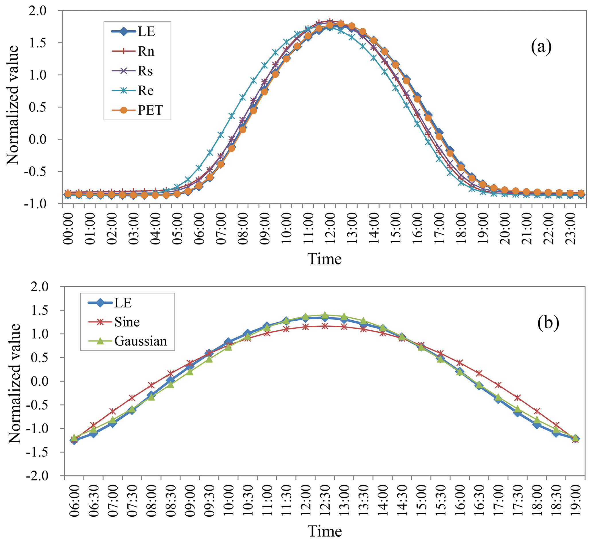
Figure 2 Intra-day distribution of normalized LE, R_n, R_s, R_e, and PET and the values from the sine and Gaussian functions.

3.2 Accuracy of seven upscaling methods in simulating daily LE series

Figure 3 presents the results from evaluating the daily LE simulations using the seven remote sensing ET upscaling methods, which include the sine and Gaussian functions, EF(R_n), EF(R_n-G), EF(R_s), EF(R_e), and EF(PET). The performance of each upscaling scheme while simulating the mean value shows that daily LE simulated by most schemes was lower than the observed values, where the underestimation was generally less than 20 %. Among them, the sine and Gaussian function methods demonstrated a relatively better performance for the mean values, where the RE was generally within ±10 %. The Gaussian and sine functions also performed the best in simulating the mean daily LE at 10:30 and 13:30, respectively. The mean values of daily LE simulated by the EF(PET) method were also relatively closer to measured values. The EF(R_n) method exhibited the poorest performance for mean daily LE simulation of all upscaling schemes. The simulated RE using this method generally ranged from 0 % to −40 %, with the mean RE of all sites being approximately −20 %. In general, there was only a small difference between upscaling simulations using the single-time value and those using multi-time values. However, the mean of simulated daily LE by the upscaling schemes at 13:30 was significantly higher than that at 10:30. The mean REs of all upscaling schemes for the former and latter time points were −2.3 % and −9.7 %, and the corresponding median REs were −1.8 % and −9.2 %, respectively. As such, the mean daily LE upscaled from 13:30 was closer to the measured value than that from 10:30; the performance of upscaling methods was better at 13:30 than at 10:30.

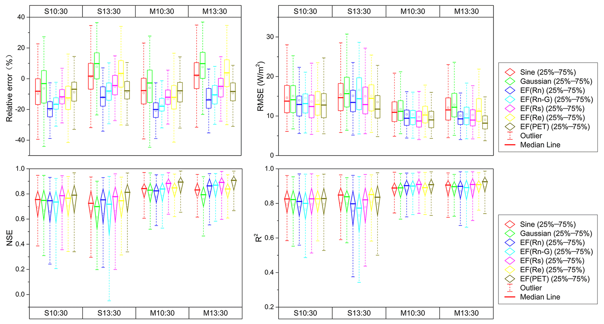
Figure 3 Simulation accuracy of daily LE using seven remote sensing ET upscaling methods, including the sine and Gaussian functions, EF(R_n), EF(R_n-G), EF(R_s), EF(R_e), and EF(PET). Note: S and M represent simulations by a single and average of multi-time values, respectively. For example, S10:30 is simulated by the ratio of a daytime value to a single-time value at 10:30, while M10:30 is simulated by the ratio of a daytime value to the average of three-time values at 10:00, 10:30, and 11:00.

The RMSE evaluation showed that the RMSE of each upscaling scheme at each site ranged from 5 to 30 W m⁻², where the mean of all simulated RMSEs was 13.5 W m⁻². In the RMSE evaluation, there was only a small difference between the upscaling simulations at 10:30 and 13:30, as opposed to the RE evaluation results. However, the simulation accuracy of multi-time values was slightly higher than the single-time value. The mean RMSEs of all upscaling schemes for the former and latter were 15.0 and 11.7 W m⁻², while the corresponding median values were 13.8 and 10.5 W m⁻², respectively.

Figure 3 also presents the evaluations based on the NSE and R² data series criteria, which evaluate the goodness of fit of the simulated and observed data series. In general, all upscaling schemes could accurately simulate daily LE series. The median NSE and R² were generally higher than 0.70 and 0.80 for all sites under each upscaling scheme, respectively. This means that the daily LE series simulated by each upscaling scheme was relatively consistent with observed values and was strongly correlated with the measured data series. Similarly to the RMSE evaluation, simulations using multi-time values were more accurate than those using a single-time value. For example, when a single-time value is used in upscaling schemes, the simulated NSE of each site mainly fell between 0.60 and 0.80. In contrast, when multi-time values were used for simulations, the NSE of each site increased to between 0.70 and 0.90, where the median exceeded 0.80. In single-time value simulations, the median of the simulated R² of all sites was approximately 0.80; when multi-time values were used, the R² improved to a value exceeding 0.90. There was a minor difference between the 10:30 and 13:30 upscaling schemes based on the NSE and R² evaluation criteria. This is because the upscaling scheme assumes that the intra-day distribution of the upscaling variable is similar to that of the observed LE. Therefore, the upscaling scheme can successfully simulate daily LE at any time during the day. However, there was significant variability in the accuracy of upscaling methods when simulated in the evening or nighttime.

A comparative analysis of the different upscaling methods was also performed. The daily LE data series simulated by the EF(PET) and EF(R_s) methods showed a relatively greater level of consistency with observed values than those simulated by the other five methods. For example, in simulations of multi-time values, the mean and median NSE simulated by the two methods at each site were 0.83 and 0.89, while the corresponding values simulated by the other five methods were 0.77 and 0.84, respectively. The RMSE evaluation results were similar to those for NSE. For example, in simulations of multi-time values, the mean and median RMSEs simulated by the two methods were 9.8 and 8.9 W m⁻², respectively, while the corresponding values for the other five methods were 11.0 and 10.3 W m⁻². In terms of the evaluation results of the correlation index R², in general, there was little difference between the performance of the seven methods. The mean R² at each site was 0.87, and the corresponding median was 0.90.

Based on this comprehensive evaluation, while the EF(PET) method was the most optimal of all seven methods, it also had the greatest input data requirements. The sine function, Gaussian function, and EF(R_e) methods, which required the least input data, also produced relatively accurate simulations. Among them, the Gaussian function method demonstrated the best performance for the mean value simulation. The EF(R_e) method was similar to the PET method as per the RMSE, NSE, and R², with a larger RE range.

3.3 Spatial distribution of the accuracy of the sine function and EF(R_e) methods

In general, all upscaling methods demonstrated an ability to accurately simulate daily LE data series at most sites, particularly for simulations using multi-time values. The spatial distribution of the accuracy of the sine function and EF(R_e) methods simulated using multi-time values was evaluated using NSE and R² (Fig. 4). The NSE of the sine function ($\mathrm{134}/\mathrm{148}$) and EF(R_e) ($\mathrm{133}/\mathrm{148}$) methods was higher than 0.60 at 90 % of sites worldwide. There were 86 and 90 sites that had an NSE exceeding 0.80 for the sine function and EF(R_e) methods, respectively. In terms of the correlation evaluation criterion, R², the number of sites in which the R² exceeded 0.80 was 117 and 121 for the two methods, respectively.

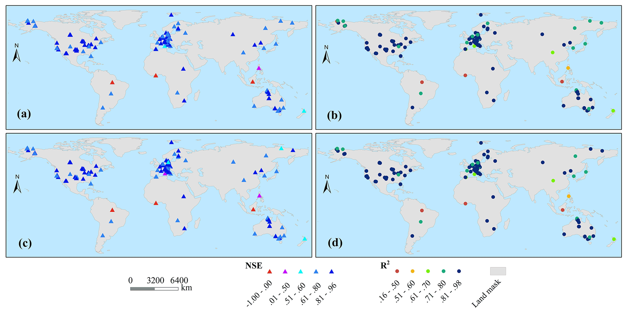
Figure 4 Spatial distribution of NSE and R² simulated by the sine function and EF(R_e) methods with multi-time values (a and b are simulated by the sine function method, and c and d are simulated by the EF(R_e) method; a and c are NSE, and b and d are R²).

Notably, in tropical rainforest (e.g., BR-Sa3, GH-Ank, ID-Pag) and tropical monsoon (PH-RiF) climatic conditions, the two methods demonstrated a poor ability to simulate daily LE. This was particularly the case for tropical rainforest climate regions, where the NSE is even lower than 0; this may be due to irregular changes in the LE in these regions. For example, there is little seasonal variation in LE in tropical rainforest climate regions, and the fluctuation of daily LE data series is relatively small. This results in poor agreement between simulated daily LE and measured values (Fig. 5). However, the SD-Dem site, also located near the Equator, was characterized by seasonal variation in LE due to the tropical grassland climate in this region. As such, the simulated daily LE at this site demonstrated greater consistency with measured values. Although the performance of upscaling methods was poor in agreement with the daily LE data, there was an apparent correlation between simulated daily LE and the measured data. For example, the R² was higher than 0.30 and 0.40 at the GH-Ank and ID-Pag sites, respectively, while it was greater than 0.50 at the PH-RiF site.

Figure 5 Observed and simulated daily LE series by the sine function upscaling method in tropical regions. Note: (a) to (c) represent BR-Sa3, GH-Ank, and ID-Pag, located in the tropical rainforest climate region; (d) and (e) are the sites of PH-RiF and SD-Dem, located in the tropical monsoon and grassland climate regions, respectively.

The spatial distribution of the accuracy of the sine function and EF(R_e) methods simulated by multi-time values was also evaluated using the RE and RMSE criteria (Fig. 6). The simulated RE at all sites ranged from −33.7 % to 24.2 %, while the RMSE was lower than 40.4 W m⁻². Most sites tended to underestimate daily LE using the two upscaling methods; this underestimation was generally less than 20 %. In East Asia, central Australia, northeastern Africa, central and northwestern North America, and southern South America, the upscaling methods underestimated daily LE by 10 %–20 %. In the Gulf of Guinea in Africa and the northeastern region of South America, both methods generally overestimated daily LE by less than 10 %. Both methods tended to underestimate the daily LE in the remaining regions by less than 10 %. The simulated RMSE of the upscaling methods exceeded 30 W m⁻² at three tropical rainforest sites and a site in southeastern Australia. The remaining sites had RMSE values below 30 W m⁻². There were 89 % ($\mathrm{132}/\mathrm{148}$) of sites with a simulated RMSE lower than 20 W m⁻².

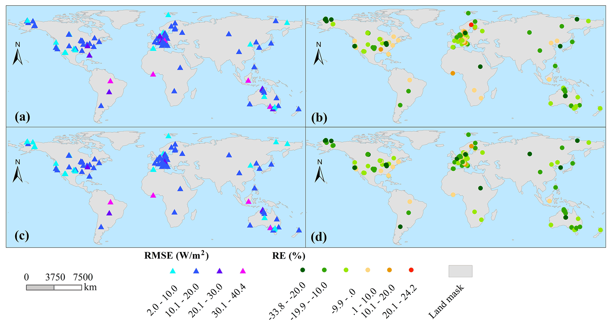
Figure 6 Spatial distribution of RE and RMSE simulated by the sine function and EF(R_e) methods using multi-time values (a and b are simulated by the sine function method, and c and d are simulated by the EF(R_e) method; a and c are RMSE, and b and d are RE).

3.4 Accuracy of upscaling schemes in simulating daily LE under all sky conditions

In this study, the simulation accuracy of upscaling methods under a different daily atmospheric transmissivity coefficient (τ) was evaluated using observed data from sites with a daily time series length greater than 1000. First, all data from these sites were constructed into a data series. Then, the accuracy of daily LE simulations using the sine function and EF(PET) upscaling methods under differing daily atmospheric transmissivity coefficients was evaluated; the results are presented in Fig. 7. In general, the simulation accuracy was positively correlated with the daily atmospheric transmissivity coefficient, particularly when τ < 0.6. The overall RE, RMSE, NSE, and R² were 6.0 % and 9.1 %, 14.3 and 11.8 W m⁻², 0.81 and 0.86, and 0.83 and 0.88 for the sine function method using the single-time value at 10:30 and the EF(PET) method using the multi-time values at 13:30, respectively. The simulation accuracy under sky conditions where τ < 0.6 was significantly lower than the overall accuracy. For example, when τ < 0.2, the two methods underestimated the daily LE by 36.7 % and 25.0 %, respectively. Although the simulation accuracy was not as high as that under large atmospheric transmissivity, the simulated NSE exceeded 0.50, even when τ < 0.2. When 0.4 < τ < 0.5, the simulated NSE had improved to exceed 0.70, and the corresponding R² was greater than 0.75. This indicates that remote sensing ET upscaling methods can achieve satisfactory simulation accuracy even when 0.4 < τ < 0.5. The simulation accuracy of the two methods was relatively stable when τ > 0.6, particularly for the EF(PET) method of multi-time values at 13:30 in which the corresponding NSE stabilized around 0.85, and R² was stable around 0.87. The RE also became relatively stable when τ > 0.6; this is consistent with the R² results, as shown in Fig. 8a and b. This indicates that the daily LE simulated by the sine function and EF(PET) upscaling methods was closer to the measured values, and the simulation accuracy of these methods was high and more reliable when τ > 0.6. The accuracy evaluation results of the other upscaling methods were similar (not shown).

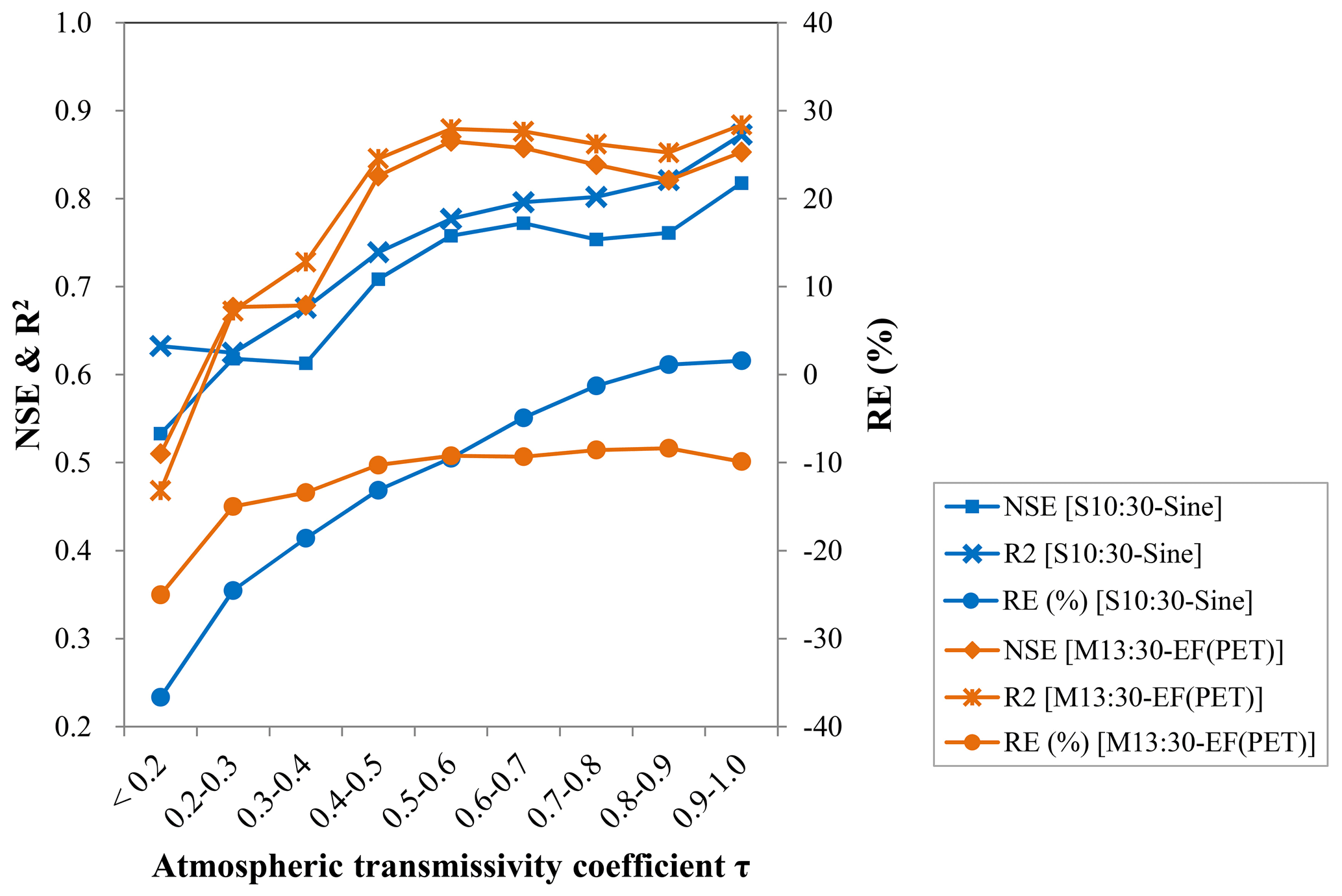
Figure 7 Overall evaluation of the sine function method simulated by a single-time value of 10:30 and the EF(PET) method simulated by multi-time values at 13:30 for all sites under differing daily atmospheric transmissivity coefficients.

Overall, under sky conditions where τ > 0.6, the upscaling schemes could simulate the daily LE series with high accuracy. However, when τ < 0.6, this simulation accuracy was significantly affected by sky conditions and was generally positively correlated with the daily atmospheric transmissivity coefficient. Although not as accurate as when atmospheric transmissivity is high (τ > 0.6), the upscaling schemes still demonstrated an ability to accurately simulate daily LE even when atmospheric transmissivity was relatively low (i.e., 0.4 < τ < 0.5).

In addition to the overall evaluation of the data series constructed across all sites, the performances of different sites under all sky conditions were evaluated. Figure 8a and b show the R² when using the sine function and EF(PET) methods under differing daily atmospheric transmissivity coefficients. In general, the R² of the upscaling methods increased with the atmospheric transmissivity coefficient; when τ > 0.6, the simulation accuracy was stable. Based on the evaluation of the EF(PET) method with multi-time values at 13:30, when τ < 0.3, the R² of each site was mainly between 0.4 and 0.7. When τ increased to between 0.3 and 0.4, the R² had increased to between 0.6 and 0.8 at most sites. When τ > 0.6, the R² of each site generally increased to greater than 0.8. Figure 8c and d show the simulated daily LE against observed values under different levels of daily atmospheric transmissivity; the simulation systematically underestimates the simulations with observed values under low levels of τ (i.e., τ < 0.2). For the instant simulation in upscaling schemes, it is important to note that simulations may be upscaled from instantaneous variables when the sky is cloudy, while the remainder of the daytime is clear. However, the opposite may also occur in which the sky conditions are clear during instant simulation and cloudy at other times.

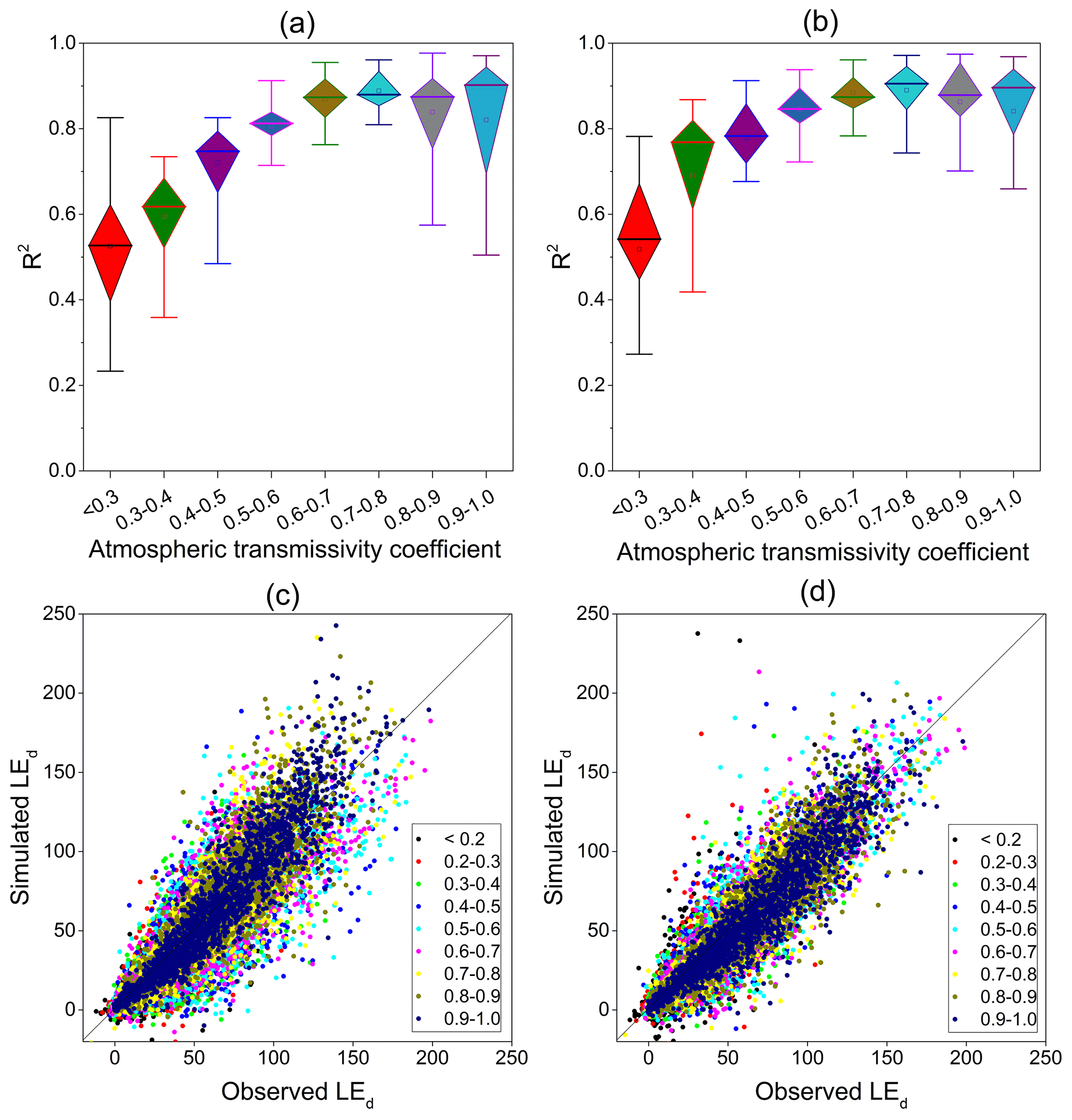
Figure 8 Box plots showing the R² of the (a) sine function method simulated by a single time at 10:30 and the (b) EF(PET) method simulated by multi-time values at 13:30 for each site. Scatter plots between observed and simulated daily LE by the (c) sine function and (d) EF(PET) methods under differing daily atmospheric transmissivity coefficients.

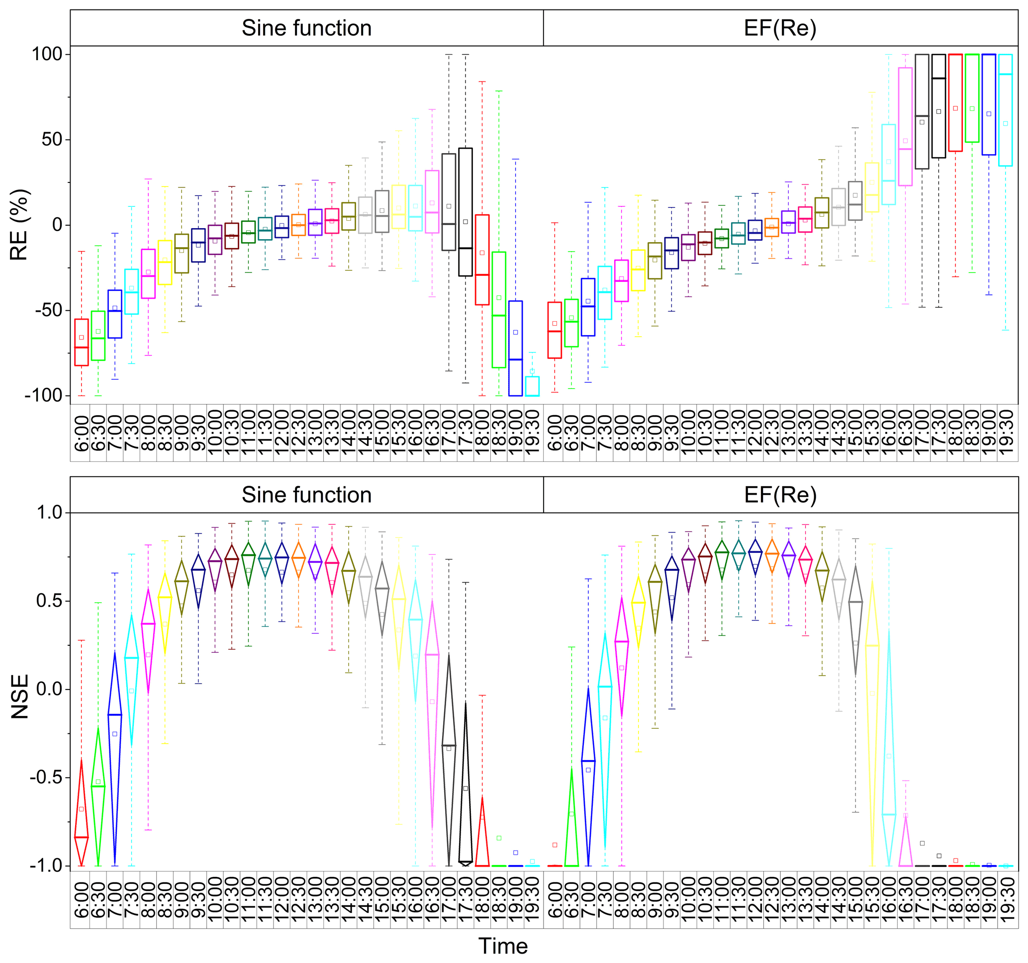
Figure 9 RE and NSE of simulated daily LE using the sine function and EF(R_e) methods at different times of the day.

3.5 Accuracy of upscaling schemes in simulating daily LE from different times of day

Remote sensing ET upscaling was conducted based on the monitoring value of the satellite overpass time; the overpass times of different satellites may vary in different regions. Therefore, the simulation accuracy of the temporal upscaling methods was also evaluated at different times of the day. Figure 9 presents the RE and NSE of the simulations using the sine function and EF(R_e) methods at different times of the day; these two methods required minimal input data. In general, the simulation accuracy of the sine function method had initially increased and then decreased during the daytime. Before 09:00, the mean RE for all sites increased linearly from −65.8 % to −14.9 %, and the RE varied significantly at each site. For example, the RE at each site ranged from −80 % to 30 % when the simulation was upscaled at 08:00. From 09:00 to 16:30, the mean RE for all sites was also increasing, although the magnitude of this increase was significantly reduced, increasing from −14.9 % to 13.0 %. During this period, the performance of the upscaling method was relatively stable, particularly during 11:00–14:00, where the RE at each site was mainly distributed from −20 % to 20 %. However, from 17:00, the mean RE showed a sharper decrease, and the performance of the upscaling method became extremely unstable at each site; this meant the RE varied significantly at each site. The daily LE was overestimated by more than 90 % at some sites, while it was also underestimated by more than −90 % at other sites. With respect to the EF(R_e) method, the RE generally showed an increasing trend during the daytime. There were three distinct stages. (1) From 06:00 to 09:00, the mean RE at all sites increases linearly from −57.6 % to −20.5 %. (2) From 09:00 to 14:30, the mean RE was also increasing, although at a lower rate from −20.5 % to 10.5 %. (3) After 15:00, the mean RE exhibits a sharp linear increase from 17.5 % to 60.3 % at 17:00 and then always exceeds 60 % thereafter.

According to the NSE evaluation criterion, the accuracy of the sine function and EF(R_e) upscaling methods in simulating daily LE data series also showed significant variability at different times of the day. The intra-day variation of NSE based on two methods at different times of the day may also be divided into three distinct stages: (1) a general linear increase before 10:00, (2) a period of relative stability from 10:00 to 13:30, and (3) a general linear decrease after 14:00. During (1), the mean NSE of all sites increased from below −0.60 to 0.60 and 0.61 for the sine function and EF(R_e) methods, respectively, while the median NSE increased from below −0.80 to 0.73 for both methods. The two methods showed the highest simulation accuracy for 10:00–13:30. In each single time point, the mean and median NSEs of all sites based on the sine function method were 0.65 and 0.74, while the corresponding values using the EF(R_e) method were 0.66 and 0.76, respectively. In addition, most sites had an NSE higher than 0.5 at single time points of 09:00, 09:30, 14:00, and 14:30. This indicates that the two methods also produce a certain accuracy in simulating daily LE at a single time point, as the mean NSE of all sites was approximately 0.50 and the corresponding median exceeded 0.60. However, the simulation accuracy of the two methods was relatively poor in the remaining periods, with a mean and median NSE lower than 0.50, particularly before 08:00 and after 16:00; in these periods, the NSE for most sites was lower than 0.20 or even lower than 0. In other words, the two methods lose the ability to upscale instantaneous LE to daily data series during these periods.

Overall, the accuracy of the sine function and EF(R_e) upscaling methods in simulating daily LE exhibits significant variability during the daytime. The simulation accuracy of both methods was relatively high from 09:00 to 15:00, with the mean REs at all sites within ±20 % and the mean and median NSEs being higher than 0.50 and 0.60, respectively. In particular, from 11:00 to 13:30, the simulation accuracy of the two methods was relatively high and stable at each site. The RE of each site was within ± 20 %, and the mean and median NSEs were 0.65 and 0.74, respectively. However, the two methods lose the ability to accurately simulate daily LE data during other times of the day, exhibiting poor simulation accuracy. Evaluation of the simulation accuracy for the other upscaling methods (not shown) at different times of the day was generally consistent with those of the sine function and EF(R_e) methods, supporting the conclusions of this study.

3.6 Variability of simulation accuracy among different upscaling schemes and sites

Based on data from 122 sites from FLUXNET2015, the standard deviation of the NSE was used to evaluate the variability of simulation accuracy among the different upscaling schemes and sites (Fig. 10). For remote sensing ET upscaling, the variability of simulation accuracy among different upscaling schemes is typically lower than the variability among different sites. At the same site, the mean standard deviation of data series composed of NSE by each upscaling scheme (the length of each series is 28, equal to the number of upscaling schemes) was 0.096. The standard deviation of the NSE by each scheme was lower than 0.20 at most sites ($\mathrm{119}/\mathrm{122}$). There were 63 % of sites ($\mathrm{77}/\mathrm{122}$) with a standard deviation of less than 0.10; these were the results for all upscaling schemes examined in this study. For the seven methods within each type of upscaling scheme (e.g., S10:30, S13:30, M10:30, or M13:30 shown in Fig. 10a), the variability of simulation accuracy among different methods was even lower, whereby the standard deviation of NSE in each scheme was less than 0.10, at more than 75 % of sites. For the simulation of multi-time values at 10:30, the standard deviation of NSE among the sine and Gaussian functions and EF(R_n), EF(R_n-G), EF(R_s), EF(R_e), and EF(PET) methods averaged only 0.052, and the number of sites with a standard deviation of less than 0.10 was up to 112 (92 %). This indicates that the variability of simulation accuracy among different upscaling schemes was relatively small for upscaling instantaneous remote sensing ET to daily values. In addition, the variability of the simulation accuracy when using multi-time values was lower than that using the single-time value.

Figure 10 Standard deviation of NSE based on (a) different methods and (b) different sites. Note: in the left-hand-side figure, S and M represent different methods by the single- and multi-time values, respectively; “All” contains all upscaling schemes used in this study. In the right-hand-side figure, the site-to-site standard deviations of simulated NSE for every upscaling scheme are shown as columns of a box plot. The five columns represent all sites where the average NSE for all upscaling schemes is higher than 0.5, 0.6, 0.7, and 0.8, and the corresponding numbers of sites are 122, 118, 111, 97, and 67, respectively.

The variability of simulation accuracy among different sites was evaluated through the site-to-site standard deviation of NSE, as shown in Fig. 10b. In each upscaling scheme, the site-to-site standard deviation of data series composed of NSE for every site (where the length of each series is 122, equal to the number of sites) ranged from 0.21 to 0.28, while the mean and median NSE of all upscaling schemes was 0.25. In each case, the variability of simulation accuracy among different sites was greater than that among upscaling schemes as the site-to-site standard deviation was always larger than the standard deviation among upscaling schemes. This higher site-to-site standard deviation is mainly due to the extremely low NSEs at several individual sites (as shown in Fig. 4). The site-to-site standard deviation significantly reduces if we exclude the four sites with an NSE lower than 0.5. For example, when only considering sites with an NSE greater than 0.5 (118), the site-to-site standard deviation is mainly distributed between 0.10 and 0.15, with mean and median values of 0.12. The site-to-site standard deviation falls below 0.09 in each upscaling scheme, when only 66 sites with an NSE greater than 0.8 were used to calculate the site-to-site standard deviation. The corresponding mean and median values of the standard deviation were 0.06. Overall, the variability of simulation accuracy among different sites was mainly affected by a limited number of sites with an extremely low NSE. Indeed, the large variations in simulation accuracy among different upscaling schemes with a standard deviation of NSE exceeding 0.20 (Fig. 10a) occurred at these four sites.

4 Discussion

In the temporal upscaling of instantaneous remote sensing ET to daily values, the current methods focus only on daytime ET. In other words, the upscaling methods only result in an ET during the daytime and do not include nocturnal ET. As for the difference in upscaled daytime LE and daily values, typically, a correction coefficient corrects this deviation. For example, Gentine et al. (2007) introduced a constant correction factor of 1.1 into the EF upscaling method; this reduced systematic underestimation and improved the performance of the method in terms of accuracy and bias for daily ET estimates (Ryu et al., 2012; Van Niel et al., 2012). In addition, time-dependent correction factors may further improve EF performance (Van Niel et al., 2011); this was also validated by the results of this study. The observation of LE at 148 global sites from FLUXNET shows that the percentage of nocturnal LE to daytime LE ranges from −2.8 % to 19.6 %, with an average of 7.8 %. The correction coefficient was calculated according to the half-hourly observed LE data series at each site; this coefficient is equal to 1 plus the ratio of nocturnal LE to daytime LE. The results show that the simulation accuracy with the correction coefficient was slightly higher than that without the correction coefficient. As such, when LE observation data become available, the correction coefficient should be used to correct the simulation of daily LE in the remote sensing ET upscaling schemes. However, hourly LE observation data are seldom available in the actual application of remote sensing ET upscaling; as such, it is necessary to consider the simulation accuracy of upscaling schemes without hourly LE data support. Therefore, the evaluation results presented in this study were simulations without any correction coefficients. In addition, note that even in the absence of LE observational data, a correction coefficient of 1.08 on the average global sites may be used to correct daily LE simulated by these upscaling methods.

The evaluation results show that the simulation accuracy of these different methods varied based on the evaluation index used. The comprehensive evaluation results show that the simulation accuracy using the EF(PET) method was the best among all seven upscaling methods. Previous studies often used reference evapotranspiration as PET in EF(PET) upscaling schemes (Trezza, 2002; Colaizzi et al., 2006; Allen et al., 2007; Cammalleri et al., 2014). The reference crop is defined as a hypothetical crop with an assumed height of 0.12 m, a surface resistance of 70 s m⁻¹ and an albedo of 0.23 (Allen et al., 1998). However, PET is related to differences in the aerodynamic properties between the reference surface and the actual landscape around the flux measurement site. In this study, PET was calculated by considering the parameters of the (bulk) surface and the aerodynamic resistance for water vapor flow based on the actual vegetation conditions at each observation site. This is more consistent with the actual situation at each site than the reference ET. However, the greatest disadvantage of this method is that it requires the input of multiple observational datasets, such as air temperature, humidity, wind speed, atmospheric pressure, crop height, and observation height. It should be noted that FLUXNET includes both raw and corrected LE data. There was little difference between the evaluation results of the corrected data and those of the raw data.

The sine function and EF(R_e) methods may be more suitable for regional remote sensing applications due to their relatively simpler inputs and comparable or higher accuracies when compared to other methods. This is consistent with the conclusions of other studies (Zhang and Lemeur, 1995; Liu and Hiyama, 2007; Van Niel et al., 2012; Ryu et al., 2012). Compared with the sine function, the intra-day distribution of LE was more consistent with the Gaussian function. However, in terms of the overall performance of upscaling methods, the simulation accuracy of the Gaussian function for daily LE did not show significant improvement. This may be mainly caused by the complementary effect between the underestimation of the sine function method around 12:00 and the overestimation of the method in the morning and afternoon. This results in an upscaled LE in the daytime by the sine function, which is similar to that of the Gaussian function.

The upscaling variable originally used by the EF method was R_n-G (Sugita and Brutsaert, 1991); in general, G is negligible in the daily energy balance (Price, 1982; Li et al., 2009; Cui et al., 2020). However, for the application of the EF method to upscale instantaneous ET to a daily scale, the instantaneous value of G is required. As R_n is also recommended in the EF upscaling method (Brutsaert and Sugita, 1992), the EF(R_n) method has been validated at several sites. For example, Van Niel et al. (2012) showed that EF(R_n) underestimated monthly ET by −16 % at two sites in Australia; the magnitude of underestimation was lower than that simulated by the EF(R_n-G) method (−34 %). In this study, the performance of the EF(R_n) and EF(R_n-G) methods in upscaling LE at 148 global sites with a long data series (including seasonal variations) was compared. The results showed that there was little difference between the simulation accuracies of the EF(R_n) and EF(R_n-G) methods; this may be good news for remote sensing ET applications. Compared to R_n, G is very difficult to detect using remote sensing (Kalma et al., 2008; Li et al., 2009), as it is usually calculated from the empirical relationship between R_n and land surface parameters (Bastiaanssen et al., 1998; Su et al., 2002; Li et al., 2019). In addition, due to the combined errors in R_n and G, the available energy (R_n-G) error estimated by remote sensing methods can reach ±10 %–20 % (Bisht et al., 2005; Kalma et al., 2008). However, if LE is only upscaled for the winter, ignoring the effect of G may produce large errors in the simulation (Cammalleri et al., 2014).

In any upscaling scheme, the simulation accuracy of multi-time values is clearly higher than that of a single-time value, which may be due to better stability in the $V_{\mathrm{d}}/V_{\mathrm{i}}$ ratio (Eq. 8) offered by the former than the latter. It is recommended that multi-time values are used in remote sensing ET upscaling when multi-time data are available. For example, if meteorological observations are selected as upscaling variables, an upscaling scheme based on multi-time values is recommended for simulations.

The spatial distribution of the simulation accuracy of each upscaling scheme showed that most sites could accurately upscale instantaneous LE to daily values. However, sites located in tropical rainforests and tropical monsoon regions performed poorly in accurately simulating daily LE, with an NSE lower than 0.20. This is consistent with the results reported by Ryu et al. (2012), who assumed that the poor performance in tropical rainforest regions was mainly due to irregular cloudiness. In addition, remote sensing products only sense the top of the canopy and thus ignore the energy storage within the canopy. Especially for forest this can be significant (Jiménez-Rodríguez et al., 2020; Coenders-Gerrits et al., 2020). This partially explains the poor performance in tropical rainforest regions. The performance of the upscaling schemes under all sky conditions was evaluated using various daily atmospheric transmissivities. High atmospheric transmissivity represents a clear-sky condition with little cloudiness. However, the simulation accuracy of these tropical rainforests and tropical monsoon regions under conditions of high atmospheric transmissivities was also low. There was little seasonal variation in LE in tropical rainforest climate regions, and the fluctuation range of daily LE data was relatively small. This may be one of the causes of the poor simulation accuracy of daily LE in these regions. Although the performance of upscaling schemes was in poor agreement with the daily LE series, it indeed showed a rough correlation between the simulated and measured daily LEs at these tropical rainforest and tropical monsoon sites.

Delogu et al. (2012) used four European flux sites to evaluate the performance of the EF(R_n-G) and EF(PET) methods at different times from 10:00 to 14:00, finding that the simulation accuracy at 11:00–13:00 was slightly higher than outside of this time range. Based on the 126 FLUXNET sites from 1999 to 2006, Wandera et al. (2017) evaluated the EF(R_s) method at different times between 10:30 and 14:00 and found that there was only slight variance in the accuracy of daily LE simulations during this period. However, the performance of upscaling methods during other daytime periods has seldom been investigated. In this study, the performance of seven upscaling methods at different times during the day (06:00–19:00) was evaluated; the simulation accuracy of upscaling methods was observed to vary significantly during the day. The upscaling methods were only able to simulate daily LE with relatively high accuracy between 09:00 and 15:00. All the methods lost their ability to accurately simulate daily LE outside of these hours. The upscaling methods exhibited the highest simulation accuracy from 11:00 to 14:00. This is consistent with previous results (Delogu et al., 2012; Wandera et al., 2017). Overall, in upscaling instantaneous ET to daily values in remote sensing applications, instantaneous values between 11:00 and 14:00 are recommended for simulations. However, if the simulation is upscaled from a time outside of 09:00–15:00, simulation accuracy cannot be guaranteed.

The performance of remote sensing ET upscaling schemes may vary significantly under different sky conditions. Wandera et al. (2017) analyzed the performance of the EF(R_s) method for four different classes of daily atmospheric transmissivity, including 0.25 $\ge \mathit{\tau }\ge$ 0, 0.50 $\ge \mathit{\tau }\ge$ 0.25, 0.75 $\ge \mathit{\tau }\ge$ 0.50, and 1 $\ge \mathit{\tau }\ge$ 0.75, where the first class represented a high degree of cloudiness and the fourth class represented clear skies. They found a relatively better simulation accuracy for the atmospheric transmissivity class above 0.75. In this study, a more refined classification of daily atmospheric transmissivity and a greater number of upscaling methods were evaluated. The results showed that the upscaling methods can simulate daily LE series with high accuracy at τ > 0.6. When τ < 0.6, the simulation accuracy of each upscaling method was significantly affected by sky conditions; accuracy was observed to be generally positively related to daily atmospheric transmissivity. However, it was also found that the upscaling methods could accurately simulate daily LE series even when the atmospheric transmissivity was relatively low (i.e., 0.4 < τ < 0.5).

Remote sensing-derived ET includes many other uncertainties, such as the uncertainty in the ET model and remote sensing data, which are indirectly related to the upscaling scheme. Although this study evaluated the accuracy of upscaling schemes in terms of simulating daily LE, in the application of remote sensing retrieval of ET, the uncertainties of remote sensing data and the ET retrieval model need to be considered.

5 Conclusion

The accuracy of seven upscaling methods in simulating daily LE from instantaneous values was evaluated using observations from 148 flux sites under all sky conditions and at different times during the day. The simulation accuracies of different methods varied based on the evaluation index that was used. All the methods could accurately simulate daily LE from instantaneous values, whereby the mean and median NSEs were 0.80 and 0.85 and the corresponding R² was 0.87 and 0.90, respectively. The sine and Gaussian function methods showed relatively higher accuracy in simulations of mean values, with REs generally within ±10 %. The EF(PET) and EF(R_s) methods showed relatively better performance in simulating daily series, where the mean and median NSEs at each site were 0.83 and 0.89, respectively. This comprehensive evaluation demonstrates that the EF(PET) method generally had the highest accuracy. However, the sine function and EF(R_e) methods may be more suitable for remote sensing upscaling applications due to their relatively minimal data requirements and comparable or higher accuracy. The intra-day distribution of the LE was more consistent with the Gaussian function than the sine function; however, the accuracy of the former method in simulating daily LE did not improve significantly compared with latter. This may be due to the complementary effect between the underestimation of the sine function method around 12:00 and the overestimation of the method in the morning and afternoon. The simulation accuracy showed little difference using the same type of method, for example, the type of mathematical function method or EF method. In any upscaling scheme, the accuracy of simulation from multi-time values was significantly higher than that from a single-time value. Therefore, multi-time values should be used in ET upscaling when multi-time data are available. The upscaling methods show the ability to accurately simulate daily LE from instantaneous values from 09:00 to 15:00, particularly for instantaneous values between 11:00 and 14:00. However, the performance of upscaling methods was poor outside of this time range. The upscaling methods could simulate daily LE with a high accuracy at τ > 0.6; when τ < 0.6, the simulation accuracy was significantly affected by sky conditions, being generally positively related to daily atmospheric transmissivity. The spatial distribution of simulation accuracy shows that every upscaling scheme has the ability to accurately simulate daily LE from instantaneous values at most sites; however, this ability is lost at tropical rainforest and tropical monsoon sites.