the Creative Commons Attribution 4.0 License.
the Creative Commons Attribution 4.0 License.
 | 11 Aug 2021
Hydrologically informed machine learning for rainfall–runoff modelling: towards distributed modelling
Herath Mudiyanselage Viraj Vidura Herath
Jayashree Chadalawada
Despite showing great success of applications in many commercial fields, machine learning and data science models generally show limited success in many scientific fields, including hydrology (Karpatne et al., 2017). The approach is often criticized for its lack of interpretability and physical consistency. This has led to the emergence of new modelling paradigms, such as theory-guided data science (TGDS) and physics-informed machine learning. The motivation behind such approaches is to improve the physical meaningfulness of machine learning models by blending existing scientific knowledge with learning algorithms. Following the same principles in our prior work (Chadalawada et al., 2020), a new model induction framework was founded on genetic programming (GP), namely the Machine Learning Rainfall–Runoff Model Induction (ML-RR-MI) toolkit. ML-RR-MI is capable of developing fully fledged lumped conceptual rainfall–runoff models for a watershed of interest using the building blocks of two flexible rainfall–runoff modelling frameworks. In this study, we extend ML-RR-MI towards inducing semi-distributed rainfall–runoff models. The meaningfulness and reliability of hydrological inferences gained from lumped models may tend to deteriorate within large catchments where the spatial heterogeneity of forcing variables and watershed properties is significant. This was the motivation behind developing our machine learning approach for distributed rainfall–runoff modelling titled Machine Induction Knowledge Augmented – System Hydrologique Asiatique (MIKA-SHA).
MIKA-SHA captures spatial variabilities and automatically induces rainfall–runoff models for the catchment of interest without any explicit user selections. Currently, MIKA-SHA learns models utilizing the model building components of two flexible modelling frameworks. However, the proposed framework can be coupled with any internally coherent collection of building blocks. MIKA-SHA's model induction capabilities have been tested on the Rappahannock River basin near Fredericksburg, Virginia, USA. MIKA-SHA builds and tests many model configurations using the model building components of the two flexible modelling frameworks and quantitatively identifies the optimal model for the watershed of concern. In this study, MIKA-SHA is utilized to identify two optimal models (one from each flexible modelling framework) to capture the runoff dynamics of the Rappahannock River basin. Both optimal models achieve high-efficiency values in hydrograph predictions (both at catchment and subcatchment outlets) and good visual matches with the observed runoff response of the catchment. Furthermore, the resulting model architectures are compatible with previously reported research findings and fieldwork insights of the watershed and are readily interpretable by hydrologists. MIKA-SHA-induced semi-distributed model performances were compared against existing lumped model performances for the same basin. MIKA-SHA-induced optimal models outperform the lumped models used in this study in terms of efficiency values while benefitting hydrologists with more meaningful hydrological inferences about the runoff dynamics of the Rappahannock River basin.
- Article
(12964 KB) - Full-text XML
- BibTeX
- EndNote


Understanding the underlying environmental dynamics occurring within watersheds is an essential and fundamental task in hydrology. Hydrological models play a key role in capturing the discharge dynamics of watersheds. Irrespective of considerable advances over past decades, there is still some scope to advance the state of the art in hydrological knowledge to fully describe the functioning of a watershed in a rainfall event owing to the highly complex, interdependent, and nonlinear behaviours of governing physical phenomena. So far, no hydrological model structure can perform equally well over the entire range of problems (Fenicia et al., 2011; Beven, 2012a). This leads to different research directions seeking different hydrological models based on different modelling strategies (Beven, 2012b). Hydrological models are expected not only to have good predictive power but also to be interpretable in capturing relationships among the forcing terms and catchment response which may lead to the advancement of scientific knowledge (Babovic, 2005, 2009; Karpatne et al., 2017). Ideally, the final goal of any successful hydrological model must be based on a physically meaningful model architecture along with a good predictive performance.
It is often observed that simple data-driven models outperform the theory-driven models, such as physics-based and conceptual models, in terms of prediction accuracy in many hydrological applications (Nearing et al., 2020). At the same time, the machine learning models are heavily criticized for the lack of interpretability of induced models (often referred to as the black box paradigm). As a result of the lack of interpretability, the contribution from data-driven models, such as machine learning models, to scientific advancement is minimal. This hindered achieving the level of success that machine learning models achieved in the commercial domain (Karpatne et al., 2017). Incorporating available scientific knowledge to guide learning algorithms to generate more physically reliable and consistent models will be an effective way to improve the explicability of machine learning models. This concept is presently recognized as a new modelling paradigm in the machine learning community as physics-informed machine learning (Physics Informed Machine Learning Conference, 2016) or theory-guided data science (Karpatne et al., 2017).
In this contribution, following the above-mentioned modelling paradigm, we introduce a novel model induction engine called Machine Induction Knowledge Augmented – System Hydrologique Asiatique (MIKA-SHA) for the automatic induction of semi-distributed rainfall–runoff models for an area of concern. This work is motivated by the success of our previously introduced (Chadalawada et al., 2020) model induction toolkit titled Machine Learning Rainfall–Runoff Model Induction (ML-RR-MI). ML-RR-MI is capable of inducing fully fledged lumped conceptual rainfall–runoff models. We use the term “hydrologically informed machine learning” to show that the existing body of hydrological knowledge is used to govern the machine learning algorithms to induce rainfall–runoff model configurations that are consistent with basic hydrological understanding. The proposed framework uses genetic programming (GP) as its learning algorithm, whereas the model building modules of two flexible rainfall–runoff modelling frameworks, namely FUSE (framework for understanding structural errors; Clark et al., 2008) and SUPERFLEX (Fenicia et al., 2011; Kavetski and Fenicia, 2011), represent the elements of existing hydrological knowledge.
By being a theory-guided data science (TGDS) approach, the top priority of MIKA-SHA remains as the induction of readily interpretable rainfall–runoff models with high prediction accuracy. However, the specific objectives of the current study involve (1) utilizing GP for semi-distributed model induction by incorporating spatial heterogeneities of catchment properties and climate variables into the rainfall–runoff modelling and (2) adopting a quantitative model selection approach to select an optimal model with appropriate complexity to represent runoff dynamics of the catchment of interest instead of the “the simpler the better” paradigm used in ML-RR-MI. The approach addresses common hydrological issues, such as equifinality, subjectivity, and uncertainty, in the context of semi-distributed modelling and machine learning. This study is a part of the larger ongoing research effort of using hydrologically informed machine learning for automatic model induction.
The following is how the rest of the text is organized. Section 1 provides a brief discussion on the background behind the development of the MIKA-SHA toolkit. The proposed model induction framework is introduced in Sect. 2. An application of the proposed framework is given in Sect. 3, followed by a discussion on research findings in Sect. 4. The last section (Sect. 5) presents the conclusions of the current study. Additional details are given in the Appendix.
1.1 Uniqueness of the place
Considering the uniqueness of the place is an important aspect of hydrological modelling (Beven, 2020). The spatio-temporal heterogeneity of landscape characteristics, such as topography, bedrock geology, soil types, land use, and climate variables, forces each watershed to behave uniquely. In general, this variability is scale dependent. More heterogeneity can be observed in both surface and subsurface levels in higher scales, such as at the catchment scale. Namely, there is a possibility that macro-scale patterns of catchments are governed by heterogeneity (Nearing et al., 2020). The use of flexible/modular modelling frameworks and distributed modelling concepts are two available toolsets for incorporating spatial heterogeneity into the model building phase.
The majority of hydrological models are developed using a generic model configuration that provides reasonable results across a relatively wide spectrum of catchments and meteorological conditions (known as fixed models). At the same time, it is quite improbable for a model to perform equally well in completely different climates and geological regions. In contrast to fixed models, modular modelling frameworks provide more flexibility in the model development by allowing the hydrologist to customize the model structure to suit the intended task. Instead of a single hypothesis available in fixed models, model building components of these modular modelling frameworks can be structured diversely to evaluate multiple hypotheses on watershed functioning. The high degree of transferability of flexible modelling frameworks is an aiding factor in proceeding in the direction of a unified hydrological theory at a watershed level. Simultaneously, due to the dynamic modularity and high level of granularity of modular modelling frameworks, constructing a suitable model for the watershed of concern may require significant effort and expert knowledge. Hence, a hydrologist with novice knowledge would be required to test many model structures before selecting an optimal model that is time demanding and computationally intensive. Consequently, it hinders the opportunity to use the flexible modelling frameworks to their full potential.
In addition to incorporating spatial heterogeneity in its modelling process, if the modeller's requirement lies within the catchment (e.g. discharge at a particular location within the catchment), then the only option would be to adopt a distributed model. At the early stages of distributed modelling, the approach (fully distributed modelling) was constrained due to the lack of data and computational power (Wood et al., 2011; Beven, 2012b; Fatichi et al., 2016). Hence, it was thought that this approach would gain success with the advancement of technology. However, until today, fully distributed models have not achieved the expected outcome (Beven, 2020). This points out that the problem lies not only in the lack of local information but is also due to the issues in how processes are represented within the distributed model (Beven, 2020). An effective alternative for fully distributed models would be the semi-distributed models, where different conceptual models are allocated to functionally distinct catchment areas. In the semi-distributed modelling approach, each model operates individually with no dependencies or interconnections with others of the network (Boyle et al., 2001; Fenicia et al., 2016). This and using conceptual models rather than small-scale physics enable semi-distributed models to be several orders simpler than fully distributed models.
1.2 Choice of the model
There is an overwhelming number of hydrological models in practice. Selecting an optimal model from among suitable competing models is not a trivial matter. According to Wainwright and Mulligan (2013), the optimal model is defined as the model with enough complexity to explain the underlying physical phenomenon. Ideally, optimal model selection should be based on bias–variance tradeoff, as the more complex models result in low bias and high variance, while simpler models result in low variance and high bias in their predictions (Hoge et al., 2018). However, there is no clear-cut definition for model complexity, and existing definitions differ across different disciplines (Guthke, 2017). In the context of hydrology, model complexity is often defined based on the process complexity and spatial complexity of the model (Clark et al., 2016), where process complexity is a measure of the number of hydrological processes explicitly represented by the model, and spatial complexity is a measure of the degree of model's spatial discretization and their connectivity.
As per the survey conducted by Baartman et al. (2019), most researchers believe selecting a model among competing models should be governed based on the question at hand (i.e. suitability of a model to achieve research objectives). However, Addor and Melsen (2019) have reported that the choice of model in hydrological applications is often based on familiarity with the model (i.e. based on legacy rather than adequacy). The inherent model complexity is frequently assessed concerning either the number of model parameters, the number of state variables, or the number of physical processes included or computational complexity, and the choice of such matrix to measure complexity is often subjective (Baartman et al., 2019). One possible alternative to measuring model complexity would be through the analysis of time series complexity of resulting output signatures of the models based on information theory and pattern matching (Sivakumar and Singh, 2012). Regardless of the matrix used to measure the model complexity, model parsimony should be a part of that as unwarranted complexity may lead to overfitting and high uncertainty (Guthke, 2017).
1.3 Machine learning in water resources
Machine learning, or data science in general, has become an irreplaceable tool not only in commercial but also in many scientific fields, with advancements in computing power and data acquisition through remote sensing and geographical information systems (Yaseen et al., 2015). Especially within the last 2 decades, there has been an increase in data science model applications, such as machine learning models, in hydrological modelling (Yaseen et al., 2015). Evolutionary computation (EC), support vector machines (SVMs), artificial neural networks (ANNs), wavelet–artificial intelligence models (W–AI), and the fuzzy set are the most popular data science techniques in hydrological modelling (Yaseen et al., 2015). Each of these techniques has its strengths and weaknesses. The scope of this paper does not discuss different data-driven methods in detail. Alternatively, interested readers may refer to the textbook by Hsieh (2009) and review articles by the ASCE Task Committee on the Application of Artificial Neural Networks in Hydrology (2000), Oyebode and Adeyemo (2014), Yaseen et al. (2015), and Mehr et al. (2018). Machine learning models have shown encouraging performances in a range of water resource applications because of their capability to handle noise complexity, nonstationarity, nonlinearity, and dynamism of data (Yaseen et al., 2015). Certainly, if we are only interested in better forecasting results, then the machine learning models might be the preferred choice over the conceptual or physics-based models (provided no data scarcity) due to their better predictive capability (Nearing et al., 2020). A machine learning model also has the advantage of requiring much less human effort to design and train than a theory-based model (Nearing et al., 2020).
Data-driven techniques have made it possible to develop implementable models with high prediction accuracy, using the available data, with limited dependence on domain knowledge. At the same time, this very nature of data-driven models has become the main point of criticism, especially in scientific fields including hydrology. They are regularly quoted as being black box models where the user has a limited understanding of how models generate their forecasts. There are two main reasons for the limited success of data-driven models in scientific fields (Karpatne et al., 2017). The first reason is the data scarcity for the model training, making it harder to extrapolate model predictions beyond the available labelled data. The second reason is associated with the objectives of scientific discovery, where the final goal is not only to have actionable models but also to convey a mechanistic awareness of underlying operations that may lead to the advancement of scientific knowledge. However, data-driven models, like deep learning (DL) models, have demonstrated better hydrograph forecasts even in ungauged basins (one of the most challenging tasks in hydrological modelling) over the conventional methods (Kratzert et al., 2019).
Not recognizing the potential of machine learning models in hydrological modelling has been identified as a danger to the hydrological modelling community (Nearing et al., 2020). Nearing et al. (2020) argue that machine learning models can identify catchment similarities by producing good performances even for the watersheds that were not utilized for training those models. This illustrates machine learning model capabilities in developing basin-scale theories that traditional models could not do so well. Furthermore, the authors refuse the most frequent critique on machine learning models (difficulties in interpretation) by arguing that even the accuracy of process representation in physics-based models is questionable owing to their poorer forecasting accuracies, so criticizing machine learning models only is unfair and meaningless. Despite having huge potential within machine learning models, state-of-the-art machine learning capacities have not yet been thoroughly explored in hydrological modelling (Shen et al., 2018). Nearing et al. (2020) expect that even distributed hydrological models are likely to be established primarily utilizing machine learning soon. Interestingly, recent studies like Nevo (2020) and Xiang and Demir (2020) have already explored the potential of DL in distributed streamflow and flood prediction, respectively. Beven (2020) emphasizes the significance of DL models' interpretability and proposes a more explicit integration of process information with DL models. Furthermore, he highlights that machine learning models should also consider issues, such as equifinality, parameter and data uncertainties, which are common in conventional modelling approaches.
1.3.1 Genetic programming (GP)
Genetic programming is an evolutionary computation (EC) algorithm (Koza, 1992) inspired through the basic principle of Darwin's evolution theory. The symbolic form of individual solution representation (known as parse trees) distinguishes GP from the other EC methods. GP is a form of supervised machine learning that allows computer programmes to be generated automatically. The ability of GP to generate explicit mathematical expressions of input–output relationships distinguishes it from other machine learning techniques. As a result, GP is referred to as a grey box data-driven mechanism, which differentiates it from the other black box data-driven approaches like ANNs (Mehr et al., 2018). Other than that, GP has become a powerful machine learning approach due to its conceptual simplicity, parallel processing capability, and ability to obtain a near-global or global solution.
GP generates its solutions (GP individuals) by arranging mathematical functions, input variables, and random constants. These are known as the building blocks of the GP algorithm. The algorithm begins with a collection of randomly generated candidate solutions for the problem to be solved. The performance of each candidate is then assessed using a user-defined objective function. Following that, genetic operators, including mutation and crossover, are performed on current generation GP individuals to produce offspring for the next generation. The procedure for selecting parent individuals for breeding guarantees that more fit individuals have a better chance of being chosen. The new set of offspring becomes the candidate solutions in the next generation. This process is repeated until the algorithm meets its termination criteria (usually a maximum number of generations). The candidate solutions evolve towards the global optimum when the GP algorithm curtails the error margin between the simulated values of its individuals and measured observations (Babovic and Keijzer, 2000).
GP has been utilized extensively in water resources, including rainfall–runoff modelling (Babovic and Keijzer, 2002; Babovic et al., 2020), meteorological data analysis (Bautu and Bautu, 2006), streamflow forecasting (Meshgi et al., 2014, 2015; Karimi et al., 2016), soil moisture estimation (Elshorbagy and El-Baroudy, 2009), water quality simulations (Savic and Khu, 2005), sediment transport modelling (Babovic and Abbott, 1997; Safari and Mehr, 2018), reservoir operations (Giuliani et al., 2015), and groundwater simulations (Datta et al., 2014).
1.3.2 Physics-informed machine learning
While the community frequently admires theory-based models (physics-based and conceptual models) owing to their explicability, which may serve to understand watershed functioning better, they often experience poorer predictive power than data science models. At the same time, simplistic applications of data-driven models, which often result in higher prediction accuracy than theory-based models, may suffer serious difficulties with interpretation as they are unable to provide basic hydrological insights (Chadalawada et al., 2020). This dichotomy led to the evolution of two major communities in water resources engineering, namely those who work with theory-based modelling and those who deal with machine learning techniques, which appear to be working quite separately (Todini, 2007; Sellars, 2018).
One promising way to bridge the gap between theory-based and machine learning modelling communities would be to couple the current hydrological understanding to govern machine learning models (Babovic and Keijzer, 2002; Babovic, 2009). This recent paradigm is presently referred to as physics-informed machine learning (Physics Informed Machine Learning Conference, 2016) or theory-guided data science (TGDS; Karpatne et al., 2017). This paradigm intends to simultaneously address the limitations of data science and physics-based models (primarily the lack of interpretability of data science models and poorer predictive capabilities of physics-based models) and to generate physically consistent and more generalizable models. According to the taxonomy presented by Karpatne et al. (2017), there are five different approaches to incorporating scientific knowledge into data science models. They are (1) theory-guided design of data science models, (2) theory-guided learning of data science models, (3) theory-guided refinement of data science outputs, (4) learning hybrid models of theory and data science, and (5) augmenting theory-based models using data science. To bring together scientific knowledge and data science techniques, a typical physics-informed data science model might use one or more of the approaches mentioned above. Only a few explainable artificial intelligence utilizations in hydrological modelling have been reported in the past (Cannon and Mckendry, 2002; Keijzer and Babovic, 2002; Fleming, 2007). However, there is an increasing trend of adopting TGDS models for recent water resource applications (Mcgovern et al., 2019), such as hydroclimatic model building (Snauffer et al., 2018), automated model building (Chadalawada et al., 2020), and hydrologic process simulation (Solander et al., 2019).
Physics-informed GP
While physics-informed machine learning is a relatively new modelling paradigm, there have been attempts over the past 2 decades to blend the hydrological understanding with the basic GP framework to improve the physical consistency of induced models. Past research, such as Babovic and Keijzer (1999, 2002) and Keijzer and Babovic (2002), used the definitions of units of measurement to bias the search process of the GP algorithm to induce dimensionally correct expressions (a so-called dimensionally aware GP). The authors examined two different approaches, namely a coercion approach (i.e. a soft constraint on dimensional correctness) and a strongly typed approach (i.e. a hard constraint on dimensional correctness) and found out that the coercion approach may be more appropriate for scientific discovery. More importantly, the dimensionally aware GP expressions were able to provide additional insights into the underlying problem. Babovic et al. (2001) utilized the dimensionally aware GP to derive hydraulic formulas from measured data and reported that GP-induced expressions are quite similar to those identified by human experts with similar or improved accuracy. In a separate study (Baptist et al., 2007; Babovic, 2009), dimensionally aware GP was used to identify expressions to describe resistance induced by vegetation and found that GP-induced expressions were superior to the expressions derived by domain experts.
Another augmented version of GP was used by Selle and Muttil (2011) to identify predominant processes in hydrological system dynamics. A reservoir model, a cumulative sum and delay function, and a moving average operator were incorporated as basic hydrological insights into the GP function set by Havlicek et al. (2013) to develop a rainfall–runoff prediction programme called SORD (Solve Or Die). They achieved superior performances in the prediction accuracy with SORD than with ANNs and GP without the above-mentioned special functions. GP was utilized by Chadalawada et al. (2017) to induce the most suitable reservoir configuration for a catchment of interest, using a customized function set with conceptual modelling concepts extracted from the Sugawara tank model architecture (Sugawara, 1979). Previously, we introduced (Chadalawada et al., 2020) an automated hydrologically informed lumped rainfall–runoff model induction toolkit, based on GP, titled Machine Learning Rainfall–Runoff Model Induction toolkit.
Chadalawada et al. (2020) introduced a new hydrologically informed rainfall–runoff model induction toolkit (ML-RR-MI) based on GP for developing lumped conceptual hydrological models utilizing model building components of FUSE and SUPERFLEX frameworks. The unique feature of ML-RR-MI is that it uses the existing body of hydrological knowledge to govern the GP algorithm to generate physically consistent models with high prediction accuracies. The building components of the two flexible modelling frameworks are used to incorporate hydrological knowledge with ML-RR-MI's learning algorithm. These building blocks are incorporated as purpose-built functions (named as FUSE and SUPERFLEX) into the function set of ML-RR-MI along with basic mathematical functions.
Successful applications of the ML-RR-MI toolkit motivated the present research to extend its modelling capabilities towards distributed hydrological modelling. Although applying the ML-RR-MI toolkit is more meaningful for small catchments due to its lumped watershed representation, there is no strict catchment size limitation for using it. However, with the increase in basin sizes, the meaningfulness of the lumped values decreases. Hence, the inferences made on the basis of a lumped model may be accurate but not reasonable or realistic. Due to the limited success and higher-order complexity of fully distributed models, the semi-distributed modelling concept is used for the current study, where a network of functionally distinguishable conceptual models from flexible modelling frameworks is developed to represent the watershed dynamics. As a result of the higher granularity and flexibility provided by the flexible modelling frameworks, even with a lumped application, one can try thousands of possible model architectures for a catchment of interest. This may rise to millions of possible model combinations in the context of semi-distributed modelling, which makes it almost impossible to test them manually.
Furthermore, selecting a model configuration without testing alternative model configurations would become highly subjective and require considerable expert knowledge and time. Upon a review of 1500+ peer-reviewed articles, Addor and Melsen (2019) reported that selecting a hydrological model is frequently based on legacy factors such as prior experience, habit, easiness, and the popularity of the model rather than adequacy factors like appropriateness of the model to achieve research objectives. A semi-distributed model choice based on a subjective model selection may introduce biased research findings. Therefore, we see a necessity to automate the model building phase to overcome these limitations. Henceforth, our machine learning approach for rainfall–runoff modelling, titled Machine Induction Knowledge Augmented – System Hydrologique Asiatique (MIKA-SHA), captures spatial variabilities and automatically induces rainfall–runoff models for the catchment of interest without any explicit user selections.
GP has been selected as the machine learning technique here due to its ability to generate an explicit mathematical relationships among independent (forcing) and dependent (response) variables. Therefore, incorporating hydrological knowledge can be done more explicitly with GP than with other black-box-type machine learning techniques. Yet, when considering most state-of-the-art GP utilizations in water resources (Oyebode and Adeyemo, 2014; Mehr et al., 2018), GP is still utilized as a short-term prediction mechanism that is analogous to ANN applications. In our contribution, we test the full potential of GP by developing fully fledged rainfall–runoff models. As MIKA-SHA relies on GP, there is no requirement for predefinition of a model structure (hypothesis on catchment runoff dynamics). Instead, identifying an appropriate model structure is part of the machine learning framework, meaning that GP simultaneously optimizes model structure and model parameters. Here hydrological insights are introduced through integrating process understanding by including model building components from existing flexible modelling frameworks into the function set of the GP algorithm. As per the classification presented by Karpatne et al. (2017), our framework falls under the hybrid TGDS category. Currently, MIKA-SHA learns models utilizing the model building components of two flexible modelling frameworks. However, the proposed framework can be coupled with any internally coherent collection of building blocks. R (R Core Team, 2018) programming language has been used to implement MIKA-SHA.
2.1 MIKA-SHA workflow
The workflow diagram of the MIKA-SHA is given in Fig. 1. Details about each module of MIKA-SHA (data preprocessing, model identification, model selection, and uncertainty analysis) are given in the sequel.
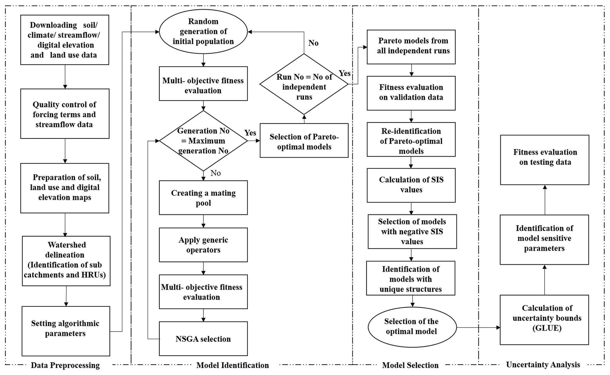
2.1.1 Data preprocessing
The data preprocessing stage includes quality checking of forcing terms (precipitation, potential evaporation, and temperature) and runoff data, identification of subcatchments and hydrologic response units (HRUs) through watershed delineation, preparation of subcatchment-averaged forcing terms vectors, and setting algorithmic parameters (e.g. number of generations, population size, number of independent runs, etc.). In general, there are no specific rules to select the appropriate algorithmic settings. However, the chosen settings eventually decide the computational time and demand. MIKA-SHA uses QGIS (quantum geographic information system) software (QGIS.org, 2020) to prepare the required digital elevation maps (DEMs), land use maps, geological maps, and soil maps for watershed delineation. Then, the SWAT+ plugin of QGIS software is used for the watershed delineation. HRUs can either be identified based on the topography, soil type, land use, and geology or a combination of different landscape types of the catchment of interest.
2.1.2 Model identification
At the model identification stage, the GP-based machine learning framework of MIKA-SHA optimizes both model structure and parameter values of candidate solutions which involve the following steps.
Step 1. A set of candidate model structures (semi-distributed model structures made from the purpose-built functions, basic mathematical functions and random constants) are randomly generated to capture the watershed's runoff dynamics (known as the initial population). These model structures (GP individuals) may differ from each other in terms of model structural components and parameter values. MIKA-SHA consists of three different initialization procedures, namely (i) the full method (all individuals have the maximum allowable initial tree depth), (ii) the grow method (individuals of different tree depths up to the maximum allowable initial tree depth are possible), and (iii) the ramped half-and-half method (individuals are generated both using the full method and grow method in equal proportions).
Step 2. The performance of each candidate model structure is evaluated on a user-defined multi-objective criterion. The non-dominated sorting genetic algorithm II (NSGA-II; Deb et al., 2002) is used to found the multi-objective optimization scheme of MIKA-SHA. Each individual in the population is evaluated on each objective function separately. MIKA-SHA utilizes parallel computation at this stage to reduce computational time.
Step 3. Each individual is assigned a non-domination rank and a crowding distance value based on the objective function values. The ranks are identified based on the Pareto optimality concept. For example, all the individuals with non-domination rank two are dominated by individuals with rank one. However, individuals with rank two are not dominated by any other individuals with a higher rank (the lower the rank, the better the individual). On the other hand, crowding distance measures how an individual is located relative to the other individuals of the same rank (the more the distance, the better the individual, and the more diversity there is).
Step 4. Individuals are selected for a mating pool to create offspring using the tournament selection mechanism (a user-defined number of individuals are chosen randomly. If they have different ranks, then the individual with the lowest rank is selected. If all of them have the same rank, then the individual with the highest crowding distance is selected). The selection mechanism ensures that individuals with higher performance values in terms of the objective functions used have a higher chance of selection.
Step 5. Genetic operators, mainly crossover (two parent individuals are divided and recombined to form two offspring) and mutation (sub-tree of a parent individual is randomly substituted with another sub-tree) are applied to parent individuals to create the child population. Then, Step 2 is followed for the child population.
Step 6. Both the parent population and child population are combined, and Step 3 is followed. Individuals are selected for the next parent population from the combined population using non-domination ranks and crowding distance values (e.g. individuals with lower ranks proceed first into the next generation until the population size is reached).
Step 7. Steps 2 to 6 are repeated until the algorithm reaches the maximum number of generations. Rank one individuals of the final generation are saved into a different file.
Step 8. Steps 1 to 7 are repeated for a user-defined number of independent runs to cover the solution space to a greater extent. The model identification stage's output consists of a set of non-dominated models (Pareto optimal models) based on the selected objective criteria.
2.1.3 Model selection
By nature, the GP algorithm drives its total population towards the global or near-global solution, which results in a set of possible solutions instead of one solution. In the context of rainfall–runoff model induction, such possible solutions may represent different model structures (different hypotheses about catchment dynamics). Identifying the best-performing model from the Pareto front of non-dominated solutions for a watershed of interest is not a trivial matter. Hence, it is often required to use a model selection scheme to select the optimal model from the competing models. The model selection stage of MIKA-SHA starts with the best models of each independent run derived through the GP framework at the model identification stage. The quantitative optimal model selection process is streamlined as follows.
Step 1. Evaluation of performance using the same multi-objective criterion on validation data for all identified models from the model identification stage.
Step 2. Re-identification of Pareto optimal models based on calibration and validation fitness performances.
Step 3. Calculation of the standardized signature index sum (SIS) of each Pareto optimal model.
Standardized signature index sum (SIS)
The SIS value is a comparative performance metric that quantifies a model's capability to capture the observed flow duration curve (FDC) relative to other competitive models (Ley et al., 2016). A model with a negative SIS value indicates an above-average capability to capture observed FDC and vice versa. In SIS calculations, both observed and simulated FDCs are divided into four flow regimes based on flow exceeding probabilities and the absolute difference in observed and simulated cumulative discharges in each region is calculated. Then, four separate Z-score values (representing four regions) are assigned to each model based on the standard deviation and mean of all models considered. The algebraic sum of those four Z-score values becomes the SIS value of the model.
where is the modulus of the signature index, where s is the model, a is FDC signature based on flow exceeding probability (FEP; FHV – FEP less than 2 %; FMV – FEP between 2 % and 20 %; FMS – FEP between 20 % and 70 %; FLV – FEP greater than 70 %), x is the value, Z is the standard score, and and σa are the average and standard deviation of .
Step 4. Selection of Pareto optimal models with SIS scores below zero over the calibration and validation periods.
Step 5. Identification of unique model structures (referred to as competitive models) from the models in Step 4. If there is more than one model with the same model structure, the model with the most negative SIS value is selected.
Step 6. Ranking of competitive models separately according to three relative measures, namely cross-sample entropy value (Cross-SampEn), dynamic time warping (DTW) distance, and model parsimony (the lower the value, the better the performance, and the lower the rank). The model with the lowest sum up rank is identified as the optimal model for the catchment in consideration.
Cross-sample entropy value (Cross-SampEn)
Cross-SampEn value is a derivation of the commonly used sample entropy value (Richman and Moorman, 2000). Sample entropy is a complexity measure of data series which has its origin in information theory. The sample entropy value gives an idea about the complexity of the data series based on the information content in a mathematical way. The Cross-SampEn value also follows the same concept but is used to measure the correlation between two series by matching patterns from one series with another. A low Cross-SampEn value indicates that the two series are more similar to each other. More details about Cross-SampEn can be found in Delgado-Bonal and Marshak (2019).
Dynamic time warping (DTW) distance
DTW distance (Sakoe and Chiba, 1978) is a similarity measure between two time series, including the warping of their time axes to find the optimal temporal alignment between the two. DTW distance is derived as an alternative to the commonly used Euclidean distance. Thus, two identical time series with a small-time shift may end up with a large Euclidean distance and may be considered as two dissimilar time series. The DTW method captures them as two similar time series as it ignores the shift in the time axes. A low DTW distance indicates more similarity between the two time series compared. Details and applications of the DTW method can be found in Salvador and Chan (2007), Giorgino (2009), and Vitolo (2015).
Model parsimony
Here, the model parsimony is evaluated in terms of each model's number of associated model parameters. One model is considered more parsimonious than another model if the number of model parameters of the former is lower than the latter.
2.1.4 Uncertainty analysis
Once the optimal model is identified for the catchment of interest, the generalized likelihood uncertainty estimation (GLUE) approach (Beven and Binley, 1992) is used to perform its sensitivity and uncertainty analysis as described below.
Step 1. A random subset of model parameters of the identified optimal model structure is uniformly changed within their parameter range (in this case, between 0 and 1 as all parameter ranges are normalized within the MIKA-SHA framework), while keeping the remaining model parameters at their calibrated values (parameter values determined in the model identification stage). Then, the performance of the parameter set is evaluated using a user-defined objective function (likelihood estimator). If the model parameter set provides an objective function value greater than the likelihood threshold, the parameter set (known as a behavioural model), its objective function value, and the simulated discharge are recorded.
Step 2. The above step is repeated until the number of behavioural models reaches a user-defined value. Each time, the number of parameters to change and which parameters to change are randomly chosen from a uniform distribution.
Step 3. For each time step, simulated discharge values of all behavioural models are sorted in ascending order. Then, a weight is assigned to each model (objective function value itself can be used as the weight). Finally, the cumulative probability distribution function (CDF) of the weights is calculated at each time step.
Step 4. For each time step, a relationship diagram is obtained by taking CDF as the x axis and simulated discharge at the y axis. From the diagram, corresponding simulated discharge values of the 95 % and 5 % quantile of CDF are selected as the upper and lower bounds of the 90 % confidence band.
Step 5. The percentage of measured streamflows of the calibration period, which fall inside the 90 % confidence band, is used to measure the uncertainty estimation capability of the selected optimal model (i.e. check whether the chosen model's parameter uncertainty is capable or not to account for total output uncertainty).
Step 6. If the uncertainty estimation capability is satisfactory (above a user-defined percent value), then the model performance of the optimal model is tested for an independent time frame (testing period) which is not used in model selection or identification stages. If the uncertainty estimation is not satisfactory, then all the above steps will be repeated with the next best competitive model.
Step 7. Sensitivity scatterplot diagrams are constructed for every model parameter using the parameter values of behavioural models. The shape of the scatterplot (the x axis – normalized parameter range; the y-axis – objective function values) is used to identify the degree of sensitivity of each model parameter.
MIKA-SHA has been developed by following good practices to handle general modelling issues related to both hydrological modelling and machine learning. Multi-objective optimization is used to ensure that the selected models perform better in many flow characteristics instead of fitting to a particular segment of measured flow. The automated and quantitative approach of the toolkit ensures no direct human involvement (no subjectivity in model induction or selection, except for setting algorithmic parameters). Model performance is evaluated on different absolute and relative performance measures. A model performing well in many performance measures may suffer less from equifinality (model performs for the right reasons). To prevent overfitting, the optimal model selection process considers performances of both calibration and validation periods. Furthermore, model parsimony is considered in the model selection stage as more complex models are more susceptible to overfitting and over-parameterization. Parallel computing significantly reduces overall computation time since purpose-built functions take much longer to compute than basic mathematical functions. The more stable fixed-step implicit Euler's method is used to solve partial differential equations.
2.2 Purpose-built functions
Incorporating existing hydrological knowledge is done by adding purpose-built functions into the function set of the GP-based optimization framework (model identification stage) of the MIKA-SHA toolkit. At present, there are two different model building block libraries in MIKA-SHA, namely the SUPERFLEX library and the FUSE library. Functional argument values of purpose-built functions decide on the structure and corresponding parameter values of induced rainfall–runoff models.
2.2.1 SUPERFLEX library
The SUPERFLEX library of MIKA-SHA includes the model building components of popular SUPERFLEX (Fenicia et al., 2011; Kavetski and Fenicia, 2011) flexible rainfall–runoff modelling framework. The SUPERFLEX framework allows hydrologists to test many different hypotheses about the functioning of the watershed of interest using the model building components (reservoirs, junctions, and lag functions) available in the framework. The water storages within the catchment, such as soil moisture, interception, groundwater, snow, and their release of water, are represented through reservoir units. Junction elements conceptualize the merging and splitting of different fluxes in catchment dynamics (e.g. Hortonian flow and evaporation). Channel routing (delays in flow transmission) is described using lag functions. A number of constitutive functions are available to describe lag function characteristics and the storage–discharge relationships of storage units (reservoirs). SUPERFLEX applications in rainfall–runoff modelling are found in van Esse et al. (2013), Fenicia et al. (2014, 2016), and Molin et al. (2020). Within MIKA-SHA, a purpose-built function named SUPERFLEX assembles these generic components in a meaningful and guided manner to induce different rainfall–runoff model structures.
2.2.2 FUSE library
The FUSE library of MIKA-SHA consists of model building components of framework for understanding structural errors (FUSE; Clark et al., 2008) modular rainfall–runoff modelling framework. FUSE was developed to examine the effect of model structural differences on rainfall–runoff modelling. FUSE conceptualizes the functioning of a catchment using a two-zone model architecture with an unsaturated zone (upper soil layer) and a saturated zone (lower soil layer). The model building modules of FUSE involve the choice of upper and lower soil configurations and parameterization for different hydrological processes, such as evaporation, percolation, interflow, surface runoff, and baseflow. The modeller has the freedom to select these model building modules from four rainfall–runoff models (TOPMODEL, ARNO/VIC, SACRAMENTO, and PRMS), which are known as FUSE parent models. For more details and applications of FUSE, please refer to Clark et al. (2011) and Vitolo (2015). Inside the MIKA-SHA FUSE library, a purpose-built function named FUSE integrates model building decisions of the FUSE framework to develop different rainfall–runoff model configurations.
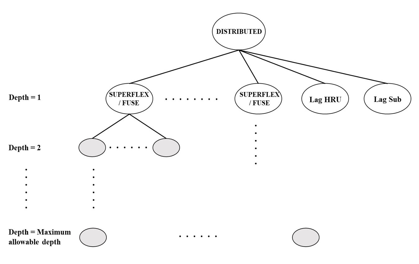
In the present contribution, a new function called “distributed” has been incorporated into the GP function set along with FUSE, SUPERFLEX and other mathematical functions. The distributed function represents the induced semi-distributed models (GP individuals) within the framework. The parse tree demonstration of the distributed function is shown in Fig. 2. As it can be seen, the distributed function uses either FUSE or SUPERFLEX functions as its function arguments, depending on the selected model inventory library by the user. The length of the function arguments of the distributed function relies on the count of HRUs within the watershed. The distributed function assigns separate model structures to each HRU, and HRUs within the same subcatchment share the same forcing variables. The last two arguments of the distributed function are the lag parameters used to route HRU outflows into the subcatchment outlets (Lag_HRU) and subcatchment outflows into the catchment outlet (Lag_Sub). Here, the routing module is based on a two-parameter gamma distribution with the shape parameter equal to 3 (Clark et al., 2008). Nodes from depth equal to 2 to depth equal to maximum allowable tree depth are the function arguments of either FUSE or SUPERFLEX functions. For more details on FUSE and SUPERFLEX functions, such as function arguments and parse tree representations, please refer to Chadalawada et al. (2020).
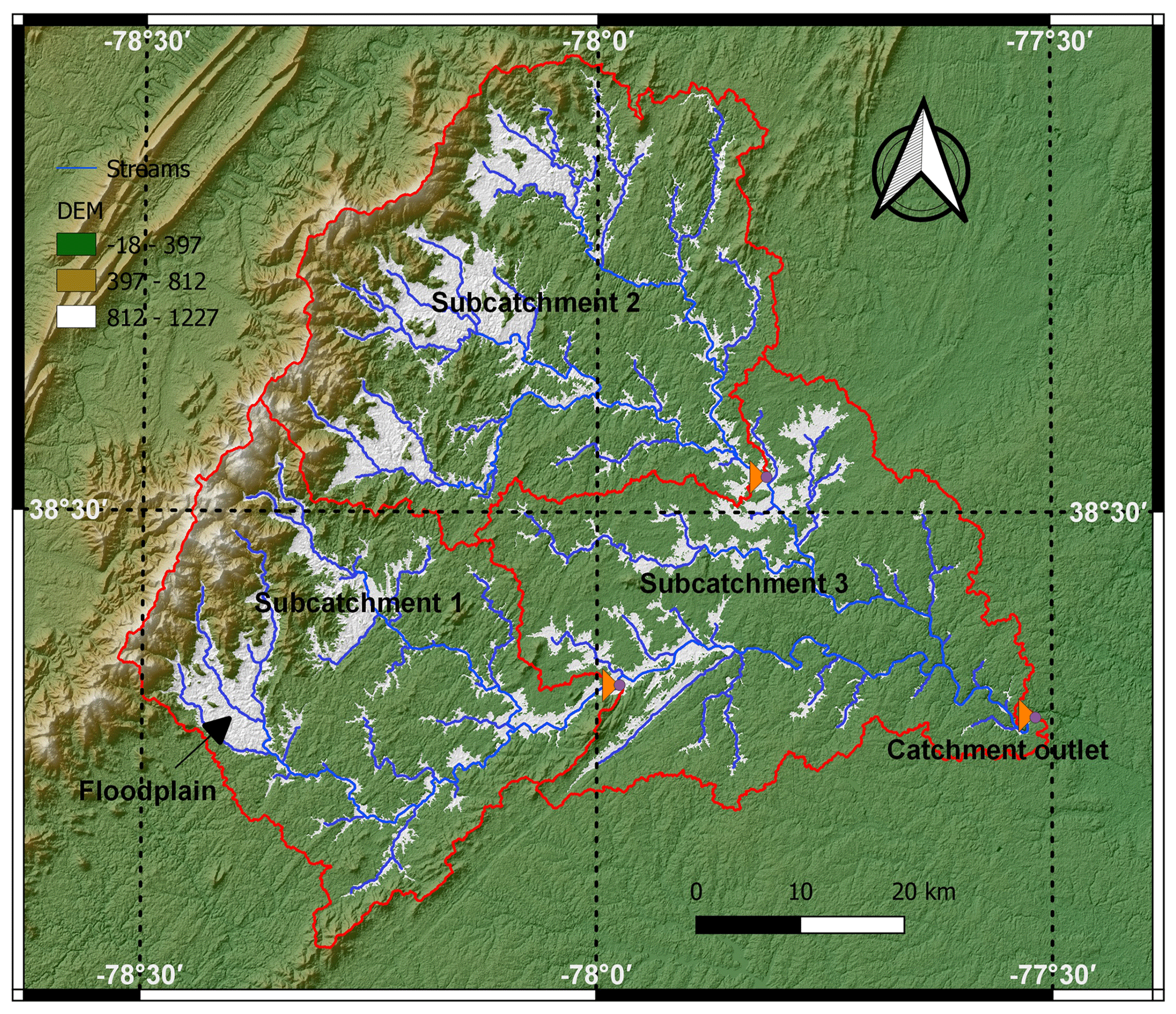
Figure 3Rappahannock River basin at Fredericksburg, Virginia, USA (map was generated through SWAT+ plugin in QGIS software using USGS EarthExplorer's Shuttle Radar Topography Mission DEM data).
2.3 Performance measures
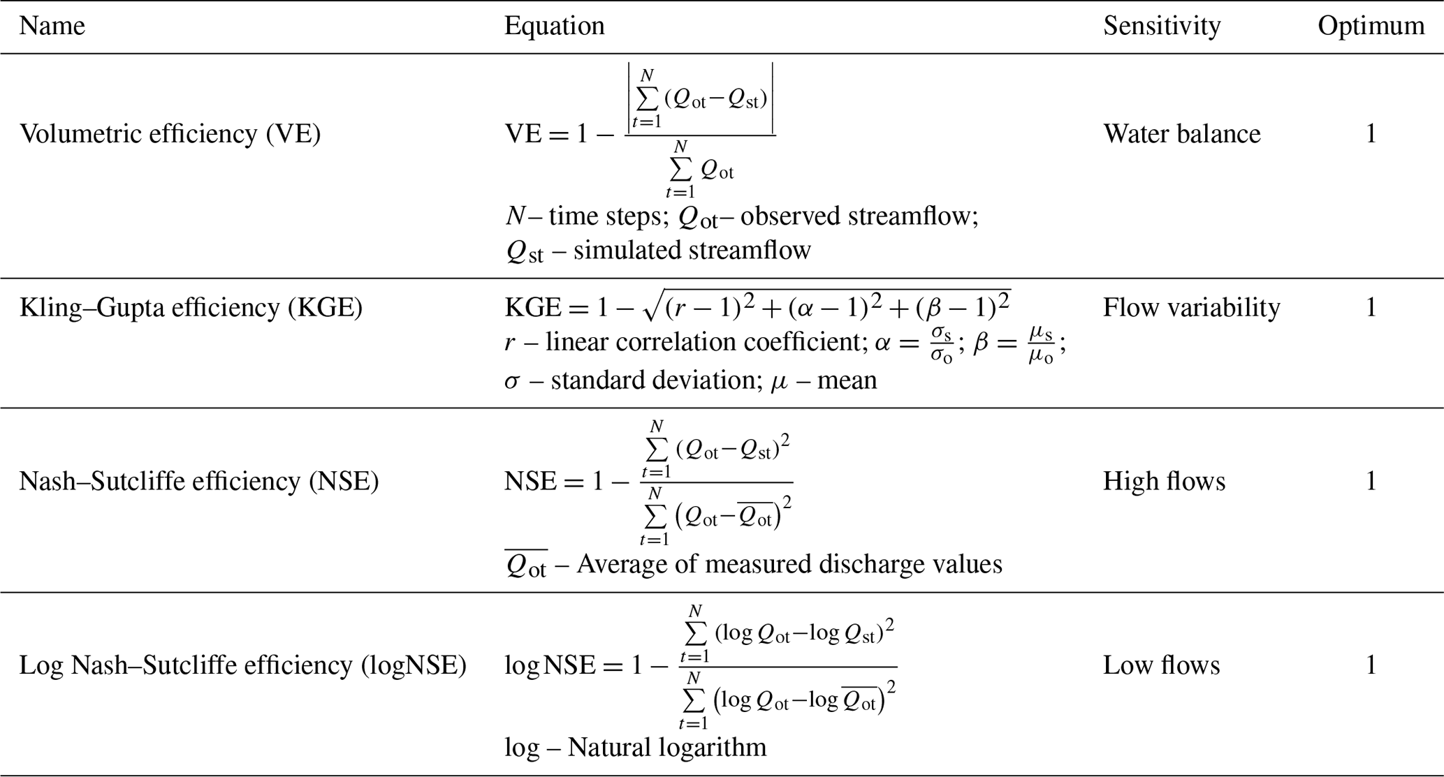
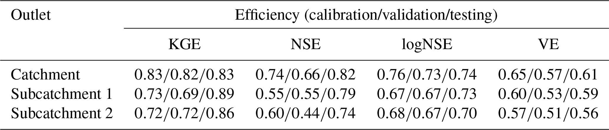
MIKA-SHA consists of a performance measures library, including the most widely adopted performance matrices. The explanatory power of the performance measure used to assess the prediction accuracy of the model simulations has a direct impact on the optimal model selection (Chadalawada and Babovic, 2017). In the present study, we have selected four absolute performance measures, namely volumetric efficiency (VE; Criss and Winston, 2008), Kling–Gupta efficiency (KGE; Gupta et al., 2009), Nash–Sutcliffe efficiency (NSE; Nash and Sutcliffe, 1970), and log Nash–Sutcliffe efficiency (logNSE; Krause et al., 2005) from the MIKA-SHA's performance measures library to evaluate the simulated discharge values against the measured discharge values. The four selected objective functions are sensitive to different regions of measured and simulated runoff signatures, and their details are given in Table 1. The four selected objective functions are used in the multi-objective optimization scheme of MIKA-SHA.
This section aims to demonstrate how MIKA-SHA works through one case study using a watershed in the USA. MIKA-SHA was applied to induce two optimal semi-distributed models for the watershed, using SUPERFLEX and FUSE model inventory libraries independently.
3.1 Study area
The Rappahannock River basin at Fredericksburg, Virginia (Fig. 3), was selected to test the semi-distributed model-induction capabilities of MIKA-SHA. Rappahannock River basin is an intermediate-scale area (ISA) river basin, with a drainage area of 4134 km2, located in the southeastern quadrant of the USA. Basin details are summarized in Table 2. Digital elevation data (DEM) of the Rappahannock River basin at 30 m resolution were obtained from the United States Geological Survey (USGS) EarthExplorer's Shuttle Radar Topography Mission (SRTM) data (USGS EarthExplorer, 2020). The entire basin was split into three subcatchments for the current application. The topography of the region was used to identify HRUs, and three HRUs, namely, Hill (slope band % > 10), Floodplain (slope position threshold = 0.1), and plateau (slope band % < 10), were selected. The HRU details are given in Table 3.
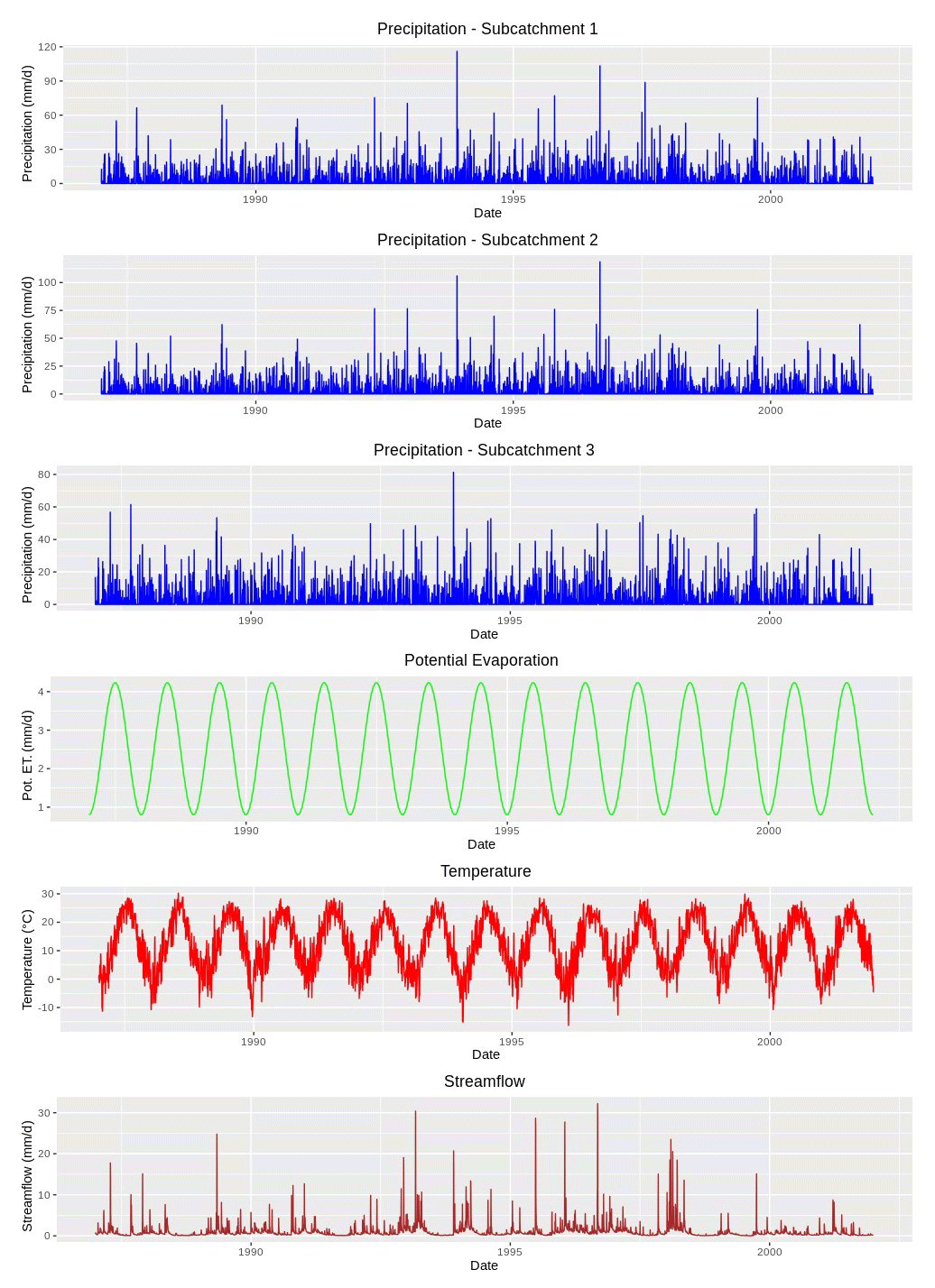
Table 1Absolute performance measures used in the current study.
In total, 15 years (1 January 1987 to 31 December 2001) of forcing terms and discharge data of the Rappahannock River basin were utilized for model spin-up (1 January–31 December 1987), calibration (1 January 1988–31 December 1992), validation (1 January 1993–31 December 1997), and testing (1 January 1998–31 December 2001). Daily catchment average potential evaporation, temperature, and streamflow data were downloaded from the MOPEX data set (USGS ID 1668000; MOPEX, 2021). The spatial distribution of daily precipitation data was taken into account and lumped at the subcatchment scale. Precipitation data were downloaded from the Daymet data set (Daymet, 2020), which provides daily weather parameters (resolution of 1 km × 1 km) over North America. The time series diagrams of precipitation, potential evaporation, temperature, and streamflow of the Rappahannock River basin are displayed in Fig. 4. Additionally, hydrometeorological data of subcatchment 1 and 2 are available in the CAMELS data set (USGS IDs 1667500 and 1664000, respectively; Newman et al., 2015). Even though MIKA-SHA only utilizes runoff at the catchment outlet for model training (calibration period), it can predict runoff at every subcatchment outlet. Therefore, once MIKA-SHA identifies the optimal models, their internal prediction capabilities are assessed using the observed runoff data of subcatchment 1 and 2. Once the relevant data are processed, the user can set the algorithmic parameters of MIKA-SHA. Table 4 summarizes the algorithmic setting of MIKA-SHA used in the current study.
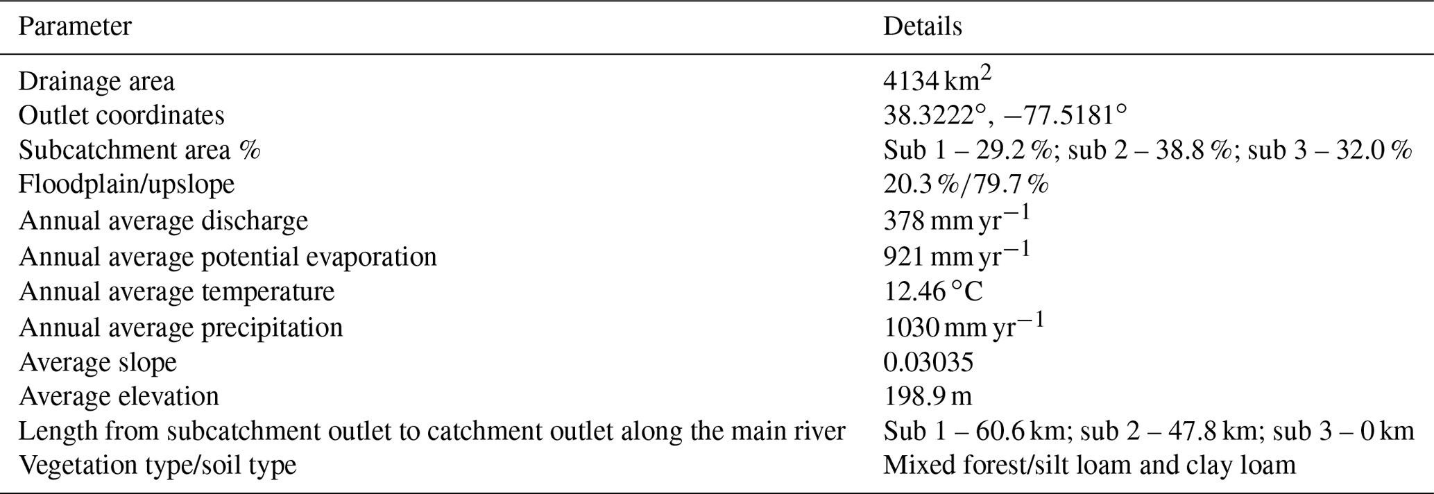

Table 4Algorithmic settings of MIKA-SHA used in the current study.
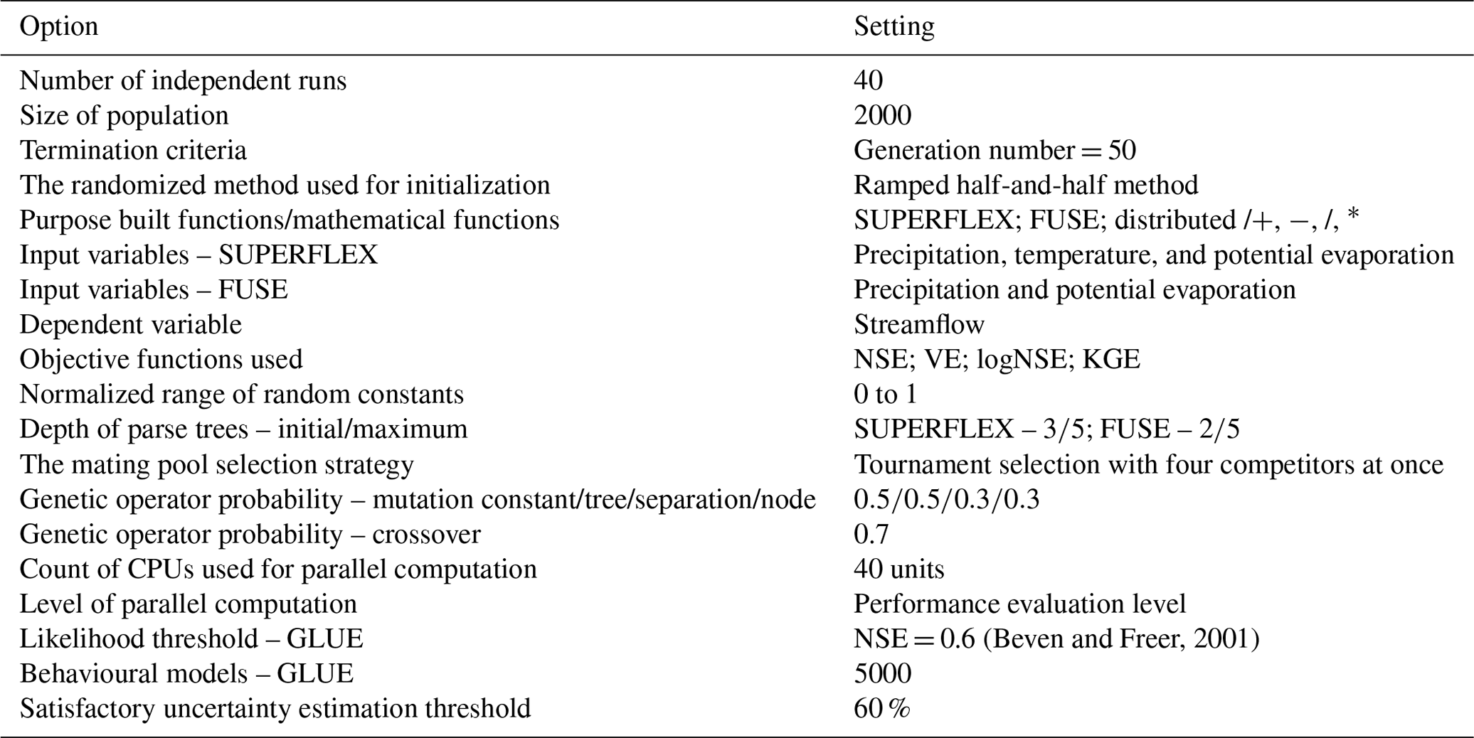
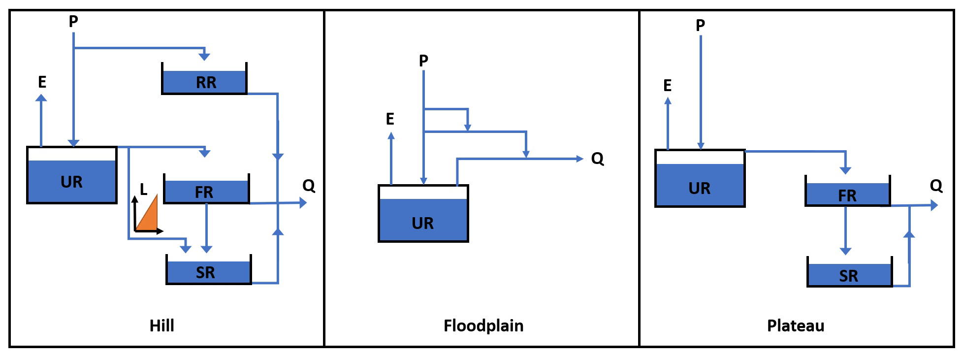
Figure 5MIKA-SHA_SUPERFLEX model configuration (P – precipitation; E – evaporation; Q – total discharge; RR – riparian reservoir; SR – slow-reacting reservoir; FR – fast-reacting reservoir; UR – unsaturated reservoir; L – half-triangular lag function).
3.2 Results
3.2.1 MIKA-SHA models induced using SUPERFLEX library
Adhering to the methodology given in Sect. 2, the model architecture presented in Fig. 5 (hereinafter referred to as MIKA-SHA_SUPERFLEX) was identified to capture the runoff response of the Rappahannock River basin. The hillside structure of the MIKA-SHA_SUPERFLEX consists of four reservoirs, i.e. a fast-reacting reservoir (FR), an unsaturated reservoir (UR), a slow-reacting reservoir (SR), and a riparian reservoir (RR). The hillside model structure also includes a half-triangular delay function associated with SR. The discharge of the UR incorporates a modified logistic curve function relationship with its storage. The storage–discharge relationships of both RR and SR are linear, while FR has a power function relationship. The model structure representing the floodplain consists only of a UR with a power function storage–discharge relationship. The second link from the top of the floodplain model structure represents the runoff generation through infiltration excess overland flow. The plateau area model structure of MIKA-SHA_SUPERFLEX is based on a three-reservoir configuration with a UR, an FR, and an SR. The power function governs the storage–discharge relationships of both UR and FR of the plateau area model structure, while the storage–discharge relationship of SR is linear.
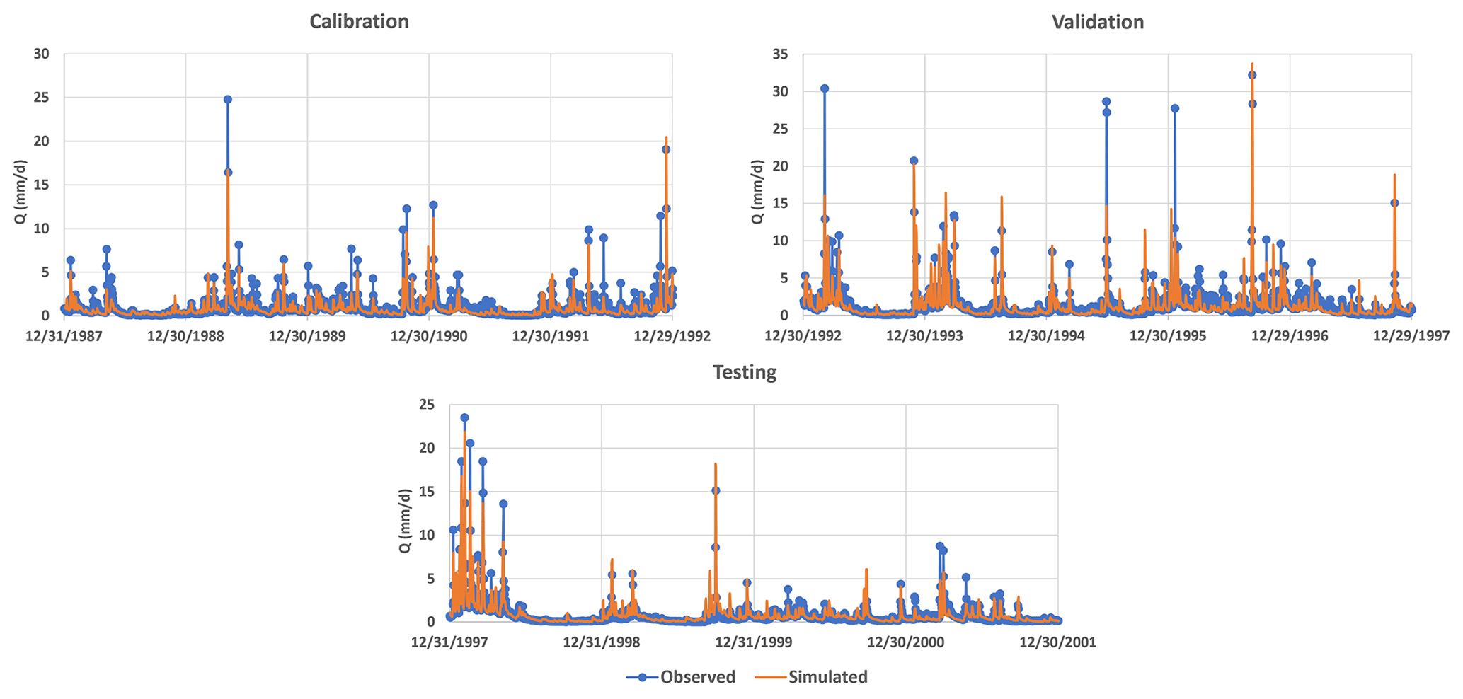
Figure 6Simulated hydrograph of MIKA-SHA_SUPERFLEX with the observed hydrograph of the basin.
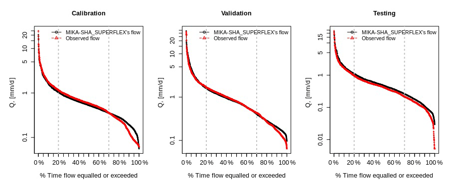
The performance matrix over the calibration, validation, and testing phases of MIKA-SHA_SUPERFLEX is given in Table 5. The high-efficiency values of all four absolute performance measures suggest that MIKA-SHA_SUPERFLEX is competent in capturing the catchment dynamics of the Rappahannock River basin. More importantly, MIKA-SHA_SUPERFLEX is capable of predicting discharge at two subcatchment outlets satisfactorily. Throughout the calibration, validation, and testing phases, the model behaves consistently. As a result, we may anticipate no overfitting problems with training data (calibration data). Figure 6 illustrates the simulated hydrograph of MIKA-SHA_SUPERFLEX along with the observed hydrograph of the watershed. As can be seen, the simulated discharge signature matches the observed discharge signature reasonably well. It is noteworthy that MIKA-SHA_SUPERFLEX underestimates the peak discharges in some instances. Figure 7 illustrates the observed FDCs of the watershed and the simulated FDCs of MIKA-SHA_SUPERFLEX for calibration, validation, and testing periods. Modelled FDCs nearly follow the measured FDCs both in medium- and high-flow regimes but diverge slightly at low-flow regimes.
Uncertainty analysis reveals that 60.2 % of the measured streamflow data of the calibration period lie inside the 90 % uncertainty bands of MIKA-SHA_SUPERFLEX, which is higher than the threshold set for the current study (60 %). Hence, it is assumed that the MIKA-SHA_SUPERFLEX's parameter uncertainty alone sufficiently estimates the total output uncertainty. Out of the 37 model parameters included in MIKA-SHA_SUPERFLEX, 13 model-sensitive parameters can be recognized by analysing the shapes of sensitivity scatterplots. A total of five of them are associated with the hillside model structure (D_R, D_F, Ce, Tlag, and Beta_Qq_UR). The floodplain model structure consists of two model-sensitive parameters (Ce and D_S), while the plateau area model structure includes four model-sensitive parameters (Beta_Qq_UR, Ce, Smax_UR, and K_Qb_FR). Furthermore, the two lag parameters of the distributed function are also identified as being model-sensitive parameters (lag_HRU and lag_Sub). The sensitivity scatterplots and the model parameter details of MIKA-SHA_SUPERFLEX are provided in the Appendix.
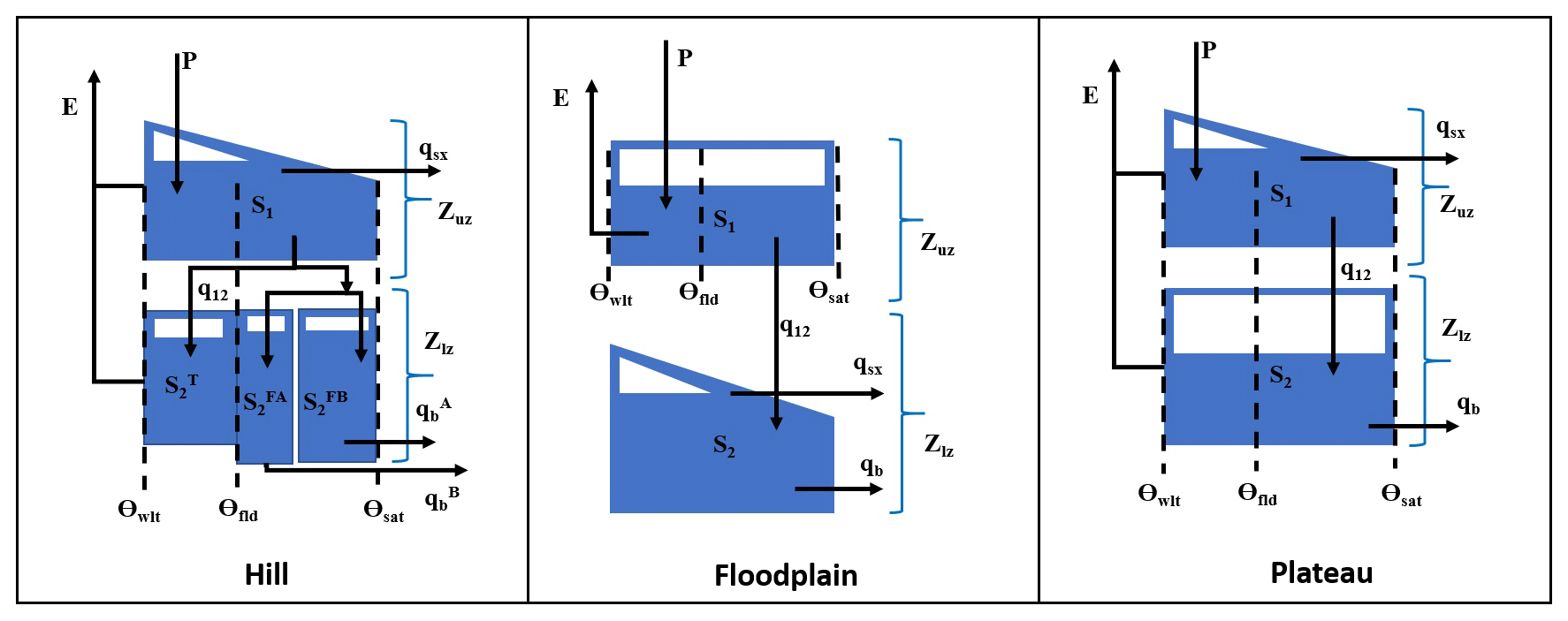
Figure 8MIKA-SHA_FUSE model configuration (P – precipitation; E – evaporation; qb – base flow; qsx – surface flow; q12 – percolation; Zuz and Zlz – depth of unsaturated zone and saturated zone; S1 and S2 – unsaturated zone and saturated zone water content; – tension water content; and : free water content in the primary and secondary baseflow storages; and – baseflow from the primary and secondary baseflow storages; Θwlt, Θfld, and Θsat – soil moisture at wilting point, field capacity, and saturation).
3.2.2 MIKA-SHA models induced using FUSE library
The identified optimal semi-distributed model for the Rappahannock River basin, using the FUSE library of MIKA-SHA, is shown in Fig. 8 (hereinafter referred to as MIKA-SHA_FUSE). Hillside, floodplain, and plateau area model structures of MIKA-SHA_FUSE, consisting of the same upper-zone configuration identical to FUSE parent model ARNO/VIC/TOPMODEL, a single-state soil reservoir. Like in the FUSE parent model of SACRAMENTO, the lower-layer architecture of the hillside model structure has a tension reservoir with two parallel tanks. The floodplain model structure incorporates a lower-zone configuration, like the FUSE parent model of TOPMODEL, with an unlimited size reservoir with power recession. In comparison, the lower-zone configuration of the plateau area model structure consists of single fixed-size storage, similar to the ARNO/VIC model. Surface flow from all three model structures is developed as saturation excess overland flow and is described using the flux equations in the FUSE parent model of TOPMODEL. Both hillside and plateau area model structures have the same percolation mechanism, allowing water to percolate from the field capacity to saturation, and is described using the flux equations of the FUSE parent model of PRMS/TOPMODEL. In contrast, percolation in the plateau area is controlled by the saturated zone's moisture amount as in the SACRAMENTO model. A root weighting evaporation model is used in hillside and floodplain model structures, while a sequential evaporation model is used in plateau area model structure. Interflow and routing are not allowed in any model structure of MIKA-SHA_FUSE.
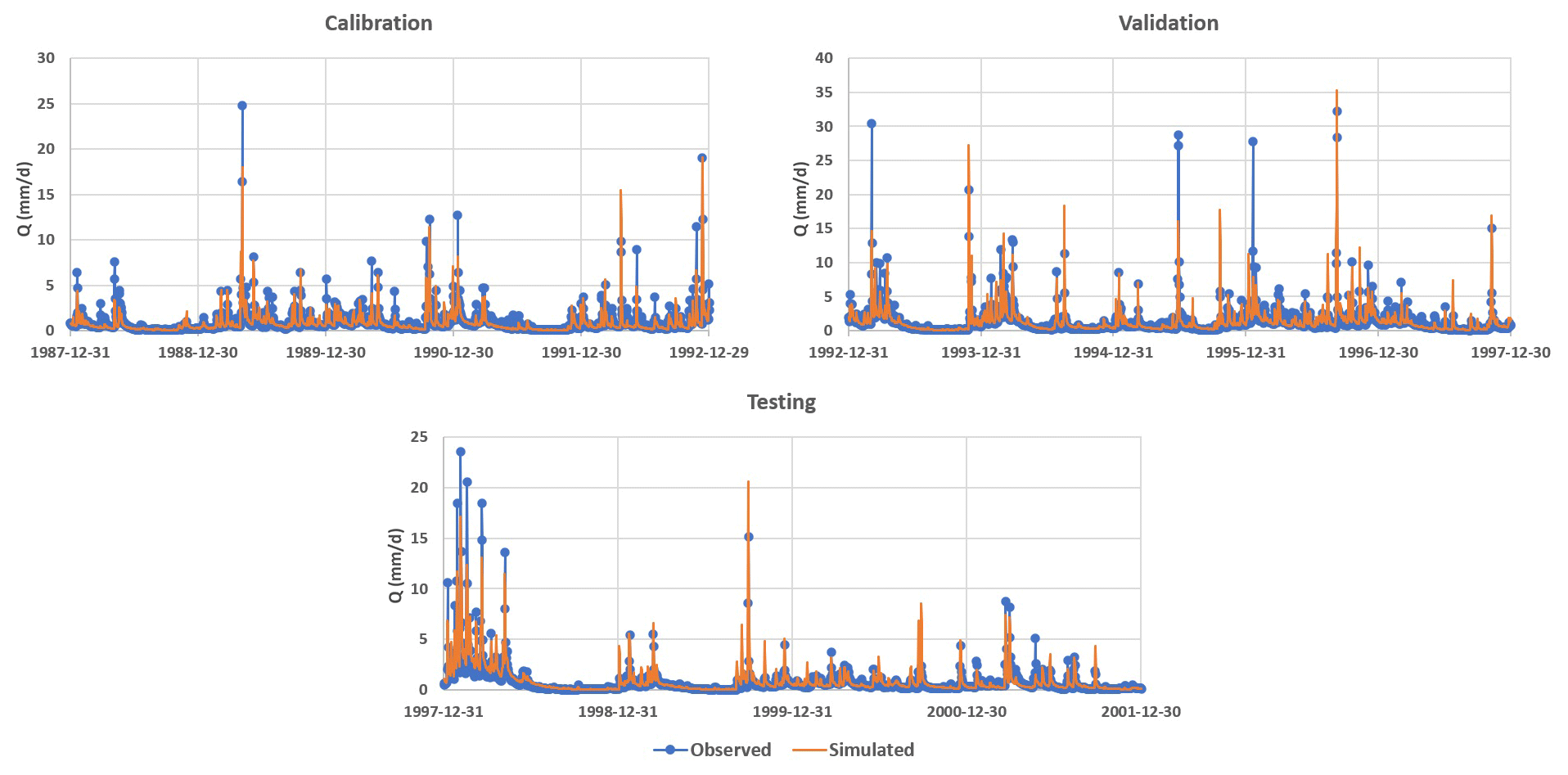
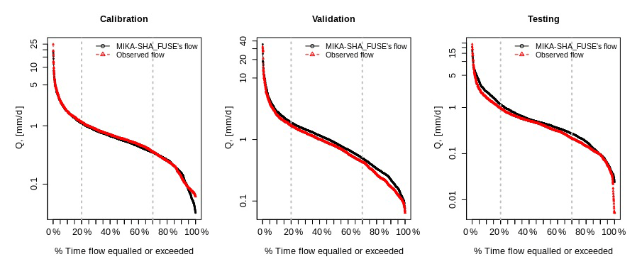
The performance matrix of MIKA-SHA_FUSE is presented in Table 6. According to the high efficiencies, the simulated discharge of MIKA-SHA_FUSE shows a good match with the observed discharge data. Furthermore, MIKA-SHA_FUSE performs consistently over the calibration, validation, and testing periods. MIKA-SHA_FUSE also demonstrates reasonable prediction accuracy for the two subcatchment outlets. Furthermore, the simulated hydrograph (Fig. 9) of MIKA-SHA_FUSE can capture the observed flow signature of the watershed reasonably well. Simulated FDCs of MIKA-SHA_FUSE are presented in Fig. 10, along with the observed FDCs of the catchment. The simulated FDC at the calibration stage nearly follows the observed FDC and deviates slightly in validation and testing periods. According to the uncertainty analysis, 82.1 % of the measured streamflows of the calibration period lie between the 90 % uncertainty bands of MIKA-SHA_FUSE. This high-percentage value suggests that the parameter uncertainty of MIKA-SHA_FUSE alone sufficiently estimates the total output uncertainty. Out of the total 34 model parameters of MIKA-SHA_FUSE, 11 model-sensitive parameters can be identified. Among them, four are related to hillside model structure (fracten, rtfrac1, percexp, and percfrac), three are related to floodplain model structure (maxwatr_1, rtfrac1, and loglamb), and two are associated with the plateau area model structure (fracten and maxwatr_2). The two lag parameters (lag_HRU and lag_Sub) are the remaining two model-sensitive parameters. Please refer to the Appendix for Sensitivity scatterplots and model parameter details of MIKA-SHA_FUSE.
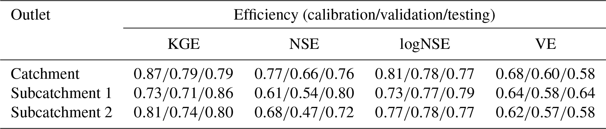
Table 7Performance matrix of Xinanjiang model and HYMOD model.
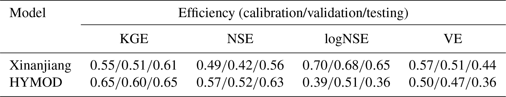
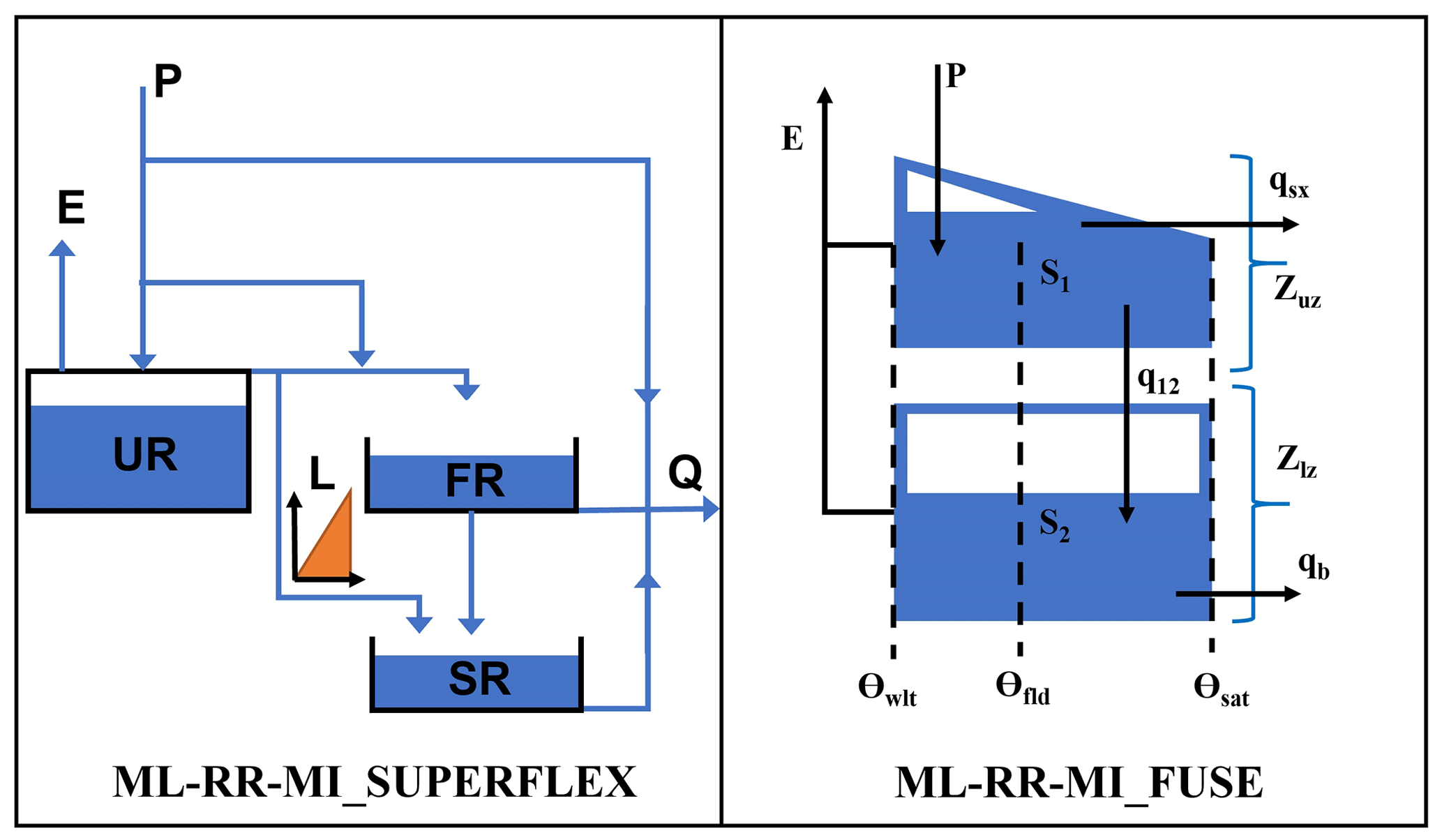
Figure 11ML-RR-MI_SUPERFLEX and ML-RR-MI_FUSE model configurations (P – precipitation; E – evaporation; Q – total discharge; SR – slow-reacting reservoir; FR – fast-reacting reservoir; UR – unsaturated reservoir; L – half-triangular lag function; qb – base flow; qsx – surface flow; q12 – percolation; Zuz and Zlz – depth of unsaturated zone and saturated zone; S1 and S2 – unsaturated zone and saturated zone water content; Θwlt, Θfld, and Θsat – soil moisture at wilting point, field capacity, and saturation).
3.2.3 Lumped vs. distributed
This section compares the optimal semi-distributed models identified by MIKA-SHA (MIKA-SHA_SUPERFLEX and MIKA-SHA_FUSE) with the lumped models calibrated/induced for the same Rappahannock River basin. First, two widely used conceptual rainfall–runoff models, namely the Xinanjiang model (Zhao, 1992) and the HYdrological MODel (HYMOD; Wagener et al., 2001), are calibrated in the lumped setting (catchment averaged forcing terms from the MOPEX data set are used) to predict the basin's catchment outflow using a non-machine learning approach. Model codes of both Xinanjiang and HYMOD models were obtained from the Modular Assessment of Rainfall–Runoff Models Toolbox (MARRMoT) framework (Knoben et al., 2019), where model codes of 46 existing hydrological models are provided. In total, two hydrological models were calibrated using the dynamically dimensioned search (DDS) algorithm (Tolson and Shoemaker, 2007) with the same model spin-up and calibration periods. DDS is a single-objective global search optimization algorithm that has been used in many hydrological modelling studies (Shafii and Tolson, 2015; Becker et al., 2019; Spieler et al., 2020). In this study, the DDS algorithm was used with NSE as the objective function. A total of 10 iterations of the DDS algorithm with 5000 model evaluations per one iteration were utilized with each model. The parameter set which gives the highest NSE over the calibration period was identified as the optimum parameter set. For the comparison purpose, VE, KGE, and logNSE values of each model (using the optimum parameter set identified with NSE) were also calculated. The performance matrix of two calibrated models is presented in Table 7. According to the efficiency values, both the Xinanjiang and HYMOD models perform poorly for the Rappahannock River basin compared to MIKA-SHA-induced semi-distributed models.
Table 8Performance matrix of ML-RR-MI_SUPERFLEX and ML-RR-MI_FUSE.

Next, our previously introduced GP-based ML-RR-MI toolkit was used to induce optimal lumped models for the same Rappahannock River basin using SUPERFLEX and FUSE libraries. ML-RR-MI was run using the same settings given in Table 4. In contrast to the MIKA-SHA, once the ML-RR-MI identifies the competitive models, the most parsimonious model in terms of the number of model parameters is recognized as the optimal model. The model configurations of the two optimal models identified by ML-RR-MI with SUPERFLEX library (hereinafter referred to as ML-RR-MI_SUPERFLEX) and FUSE library (hereinafter referred to as ML-RR-MI_FUSE) are shown in Fig. 11. ML-RR-MI_SUPERFLEX is similar to the plateau area model structure of MIKA-SHA_SUPERFLEX regarding the reservoir units and storage–discharge relationships. Additionally, ML-RR-MI_SUPERFLEX consists of a half-triangular lag function with SR. Interestingly, ML-RR-MI_FUSE's upper- and lower-layer architectures and percolation mechanism are similar to the plateau area model structure of MIKA-SHA_FUSE. In contrast, surface runoff of ML-RR-MI_FUSE is controlled by the upper layer, and the evaporation module is root weighting as in FUSE parent model ARNO/VIC. Furthermore, routing is also allowed in ML-RR-MI_FUSE.
The performance matrix of ML-RR-MI_SUPERFLEX and ML-RR-MI_FUSE is given in Table 8. In contrast to the two fixed conceptual models (Xinanjiang and HYMOD), two optimal lumped models identified by ML-RR-MI demonstrate higher prediction capabilities. MIKA-SHA_FUSE model outperforms the ML-RR-MI_FUSE model in all four objective functions over the calibration, validation, and testing periods. However, the ML-RR-MI_SUPERFLEX model outperforms or performs the same as the MIKA-SHA_SUPERFLEX model in the calibration and validation periods. Yet, the MIKA-SHA_SUPERFLEX model outperforms ML-RR-MI_SUPERFLEX in all objective functions over the testing period. As per the workflow of both MIKA-SHA and ML-RR-MI, calibration and validation periods are used in the optimal model identification process. Therefore, the performance in the testing period demonstrates the out-of-sample performance of induced models.
4.1 MIKA-SHA_SUPERFLEX
Among the three model structures of MIKA-SHA_SUPERFLEX, the hillside model structure has the most complex configuration in terms of reservoir units and model parameters. Furthermore, the hillside model structure is correlated with the majority of model-sensitive parameters, and runoff per unit area is also highest in the hillside model structure. Therefore, runoff generation from the hillside structure is a significant component of the total runoff of MIKA-SHA_SUPERFLEX. This is quite meaningful due to the higher topographic gradients in upper subcatchments (subcatchment 1 is 23.4 m km−1 and subcatchment 2 is 30.3 m km−1) of the Rappahannock River basin.
On the other hand, the plateau area model structure has the lowest runoff generation per unit area (i.e. highest storage). We find this behaviour of the plateau area model structure reasonable as a more subsurface-oriented delayed response may be expected in the plateau area due to milder slopes which may result in higher residence times (water may have more time to reach deeper soil layers). Furthermore, most of the catchment area of the Rappahannock basin consists of moderately permeable silty loam and clay loam soils which may also encourage vertical drainage. Conceptually, SRs are used to represent the slow runoff components like groundwater flow. SRs in both the hillside and plateau area model structures have linear storage–discharge relationships. Interestingly, it is reported that (Fenicia et al., 2006) linear reservoirs best describe the slow flow dynamics of groundwater movement. Furthermore, the inclusion of stable baseflow components (SRs in both hillside and plateau area model structures) in the model configuration of MIKA-SHA_SUPERFLEX is reasonable because the main river channel of the basin can be categorized as a perennial river where a continuous groundwater supply is required to sustain water throughout the year.
The floodplain model structure of MIKA-SHA_SUPERFLEX has a relatively simple model architecture with only one reservoir. The floodplain area is expected to be saturated or nearly saturated and continuously connected with the stream. In earlier FLEX and SUPERFLEX applications (Savenije, 2010; Fenicia et al., 2016), where the model selection for each HRU was based on expert judgement, a simple linear reservoir model was identified as being sufficient enough to represent quick runoff responses of riparian zones. Consistent with this in the current application, MIKA-SHA also identified a simpler model with one reservoir to capture the runoff dynamics of floodplains. However, the UR in the floodplain model structure has a power function relationship between its discharge and storage. As mentioned earlier, infiltration excess overland flow is included as a runoff component of the floodplain model structure. Often floodplains consist of soil types with poor permeabilities and, hence, may cause quick runoff generation mechanisms like infiltration excess overland flow. The constitutive functions of FRs and URs in MIKA-SHA_SUPERFLEX are nonlinear, which may help capture the nonlinear and threshold-like response of runoff generation.
4.2 MIKA-SHA_FUSE
The hillside model structure of MIKA-SHA_FUSE has the highest runoff generation per unit area (approximately 2.1 × plateau area runoff generation), followed by the floodplain model structure (about 1.6 × plateau area runoff generation). Interestingly, a similar order was observed with MIKA-SHA_SUPERFLEX. Similar to the hillside model structure of MIKA-SHA_SUPERFLEX, the hillside model structure of MIKA-SHA_FUSE has the most complex model configuration in terms of the number of model parameters and is associated with most of the model-sensitive parameters. Hence, it is clear that runoff generation from the hillside model structure dominates the total runoff generation of MIKA-SHA_FUSE, which is logical due to the high topographic relief of the basin. Furthermore, a high runoff generation in the floodplain model structure is meaningful due to high water table levels in floodplains, resulting in quick runoff generation mechanisms like saturation excess overland flow. Comparatively, lower percolation can be expected in the floodplain model structure as its percolation is controlled by the moisture content in the lower zone (percolation is higher when the lower zone is dry). This is in line with the characteristics of floodplains, which remain saturated or nearly saturated most of the time.
On the other hand, a comparatively lower runoff contribution from the plateau area model structure is reasonable as more vertical drainage can be expected than lateral drainage in plateau areas due to milder slopes and moderately permeable soil types. As per the calibrated model parameters and model-sensitive parameters, runoff from the plateau area model structure is dominated by the subsurface flow component. Lower-layer reservoirs of both the floodplain and plateau area model structures consist of nonlinear storage–discharge relationships (baseflow), which may help them capture the nonlinear runoff response of the Rappahannock River basin. In contrast, baseflow from the hillside model structure is generated through two parallel linear reservoirs.
4.3 Model induction capability of MIKA-SHA
The proposed MIKA-SHA toolkit incorporates spatial heterogeneity in catchment properties and forcing terms into the model building phase and induces representative semi-distributed rainfall–runoff models based on measured data to capture the discharge response of the watershed of interest. In comparison to the lumped model performances presented in Sect. 3.2.3, two optimal semi-distributed models, identified by MIKA-SHA with FUSE and SUPERFLEX libraries, achieve higher efficiency values, especially for the testing period. The difference in efficiency values is significant between MIKA-SHA-induced semi-distributed models and two fixed lumped hydrological models (Xinanjiang and HYMOD). MIKA-SHA-induced semi-distributed models may achieve higher-efficiency values than fixed hydrological models used in this study due to (i) the flexibility offered by modular modelling frameworks for customizing the model structure in contrast to the single model structure in fixed hydrological models, (ii) the incorporation of spatial heterogeneity in catchment properties and climate variables, and (iii) the capability of the GP based machine learning framework to optimize both model structure and parameters over the non-machine learning method.
Even though the two fixed lumped models could not achieve satisfactory performance, two lumped models induced by our previously introduced ML-RR-MI toolkit performed well in capturing the Rappahannock River basin runoff response. This demonstrates the capability of lumped models to perform satisfactorily, even for large catchments with substantial spatial heterogeneities. However, the inferences gained through a lumped model for a large watershed may be limited, and the lumped representation may not reflect the physical reality in runoff generation. As seen with MIKA-SHA_SUPERFLEX and MIKA-SHA_FUSE, the inferences made through the semi-distributed models are much more meaningful and compatible with catchment characteristics. On top of that, MIKA-SHA-induced models have a unique advantage over the lumped models for predicting discharge inside the watershed (at subcatchment outlets).
In this study, the spatial heterogeneity of the catchment was incorporated into the model building process based on the topography (i.e. three HRUs, namely hills, floodplain, and plateau, were identified based on the topography of the area). The results obtained based on topography-based HRUs, such as achieving higher-efficiency values for the absolute performance measures and obtaining a good visual equivalent between measured and modelled hydrographs, suggest that the topography of the catchment may have a strong impact on runoff generation. This illustrates another potential utilization of MIKA-SHA when using the toolkit to identify the runoff drivers of a catchment of interest. For example, one can also define the HRUs based on either the geology or soil type of the catchment of interest and use MIKA-SHA to identify optimal model configurations. This way, one can determine the relative dominance of runoff drivers towards the total catchment runoff response.
One of the major issues with machine learning models is the overfitting of the model to its training data set. However, the optimal model selection strategy used in MIKA-SHA, which considers both calibration and validation model performances, ensures the selected optimal model performs satisfactorily – and not only in the training period (more generalizability). Deterministic semi-distributed modelling would require or rely on a large number of model parameters, by comparison, and a smaller number of model parameters are sensitive to the total model performance. Furthermore, the values of two lag parameters associated with the distributed function (lag_HRU and lag_Sub) were found to be crucial in achieving high model performances. As the research findings of MIKA-SHA demonstrate a logical match with previously reported research findings and fieldwork insights, it may be safe to assume that MIKA-SHA is capable of handling the equifinality phenomenon satisfactorily (i.e. selected optimal models perform for the right reasons). Additionally, the quantitative model selection scheme of MIKA-SHA ensures that the selected optimal model has the appropriate complexity to describe the dominant runoff-generation processes of the catchment instead of selecting an optimal model only based on model parsimony.
More importantly, both MIKA-SHA_SUPERFLEX and MIKA-SHA_FUSE share similarities among their model configurations, such as model outflows dominated by the runoff generated through hillside model structures, having the most complex configurations for hillside model structures, and demonstrating more subsurface-type delayed responses by plateau area model structures. Furthermore, finding a reasonable match between the model structural components of optimal models and the catchment characteristics was possible. The consistency and compatibility demonstrated by the MIKA-SHA in capturing similar runoff dynamics across different model inventories show that the toolkit is capable of extracting information from data, making it feasible to depend on the derived model configurations beyond just statistical confidence.
In this contribution, we introduce Model Induction Knowledge Augmented-System Hydrologique Asiatique (MIKA-SHA) for learning semi-distributed models, where the spatial distributions of catchment properties and climate variables are taken into account. MIKA-SHA utilizes existing hydrological knowledge to guide the machine learning algorithm, which eventually results in physically meaningful hydrological models that can be readily interpretable by domain specialists. In the current study, background hydrological knowledge is blended with the machine learning algorithm through the model building components of flexible rainfall–runoff modelling frameworks.
Results of this study indicate that the consideration of spatial distributions of forcing data and catchment properties gives more meaningful insights regarding the environmental dynamics occurring within the watershed. MIKA-SHA's unique and distinct feature is that it can be combined with any internally coherent set of building blocks reflecting the hydrological knowledge elements. Furthermore, it uses genetic programming to optimize both model architecture and model parameters simultaneously. This approach enables hydrologists to utilize flexible modelling frameworks to their full potential by trying many hypotheses before selecting an optimal model. By automatically identifying optimal model structures for a catchment of interest that relies on adequacy instead of legacy, MIKA-SHA can serve as an alternative to the conventional subjective model selection. MIKA-SHA is expected to be most valuable in circumstances where there may be a lack of experimental insights regarding the catchment of interest or a lack of expert knowledge.
We see machine learning algorithms as having great potential in hydrological modelling. However, simplistic black-box-type data-driven models may contribute to developing accurate models with severe interpretation difficulties that may not advance hydrological understanding. Thus, the most promising way forward would be to integrate current hydrological understanding with learning algorithms to generate physically consistent and more generalizable models. This was the driving force behind the proposed MIKA-SHA framework's development, which has been founded on both machine learning and hydrological theories. As a result, we anticipate that current research will reinforce the connection between two important but traditionally separate communities in water resources, i.e. those operating with machine learning and those dealing with theory-based modelling. Finally, we foresee that more theory-guided machine learning research in hydrological modelling will be geared towards automated model building and knowledge discovery.
Table A1Model parameter details of ML-RR-MI_SUPERFLEX and MIKA-SHA_SUPERFLEX.

* For more details, please refer to Fenicia et al. (2016).
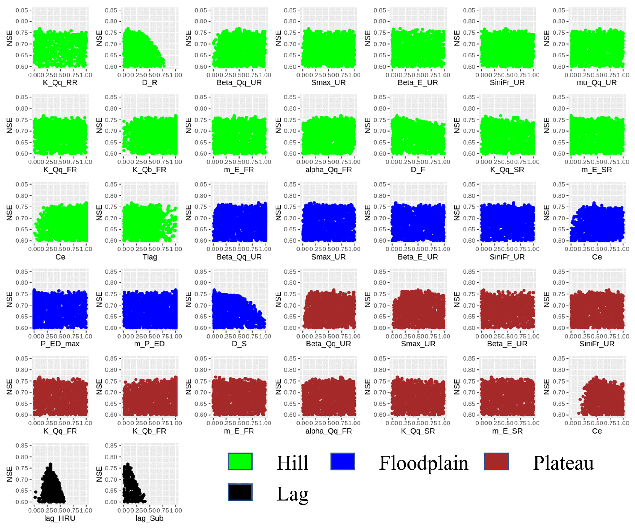
Table A2Model parameter details of ML-RR-MI_FUSE and MIKA-SHA_FUSE.
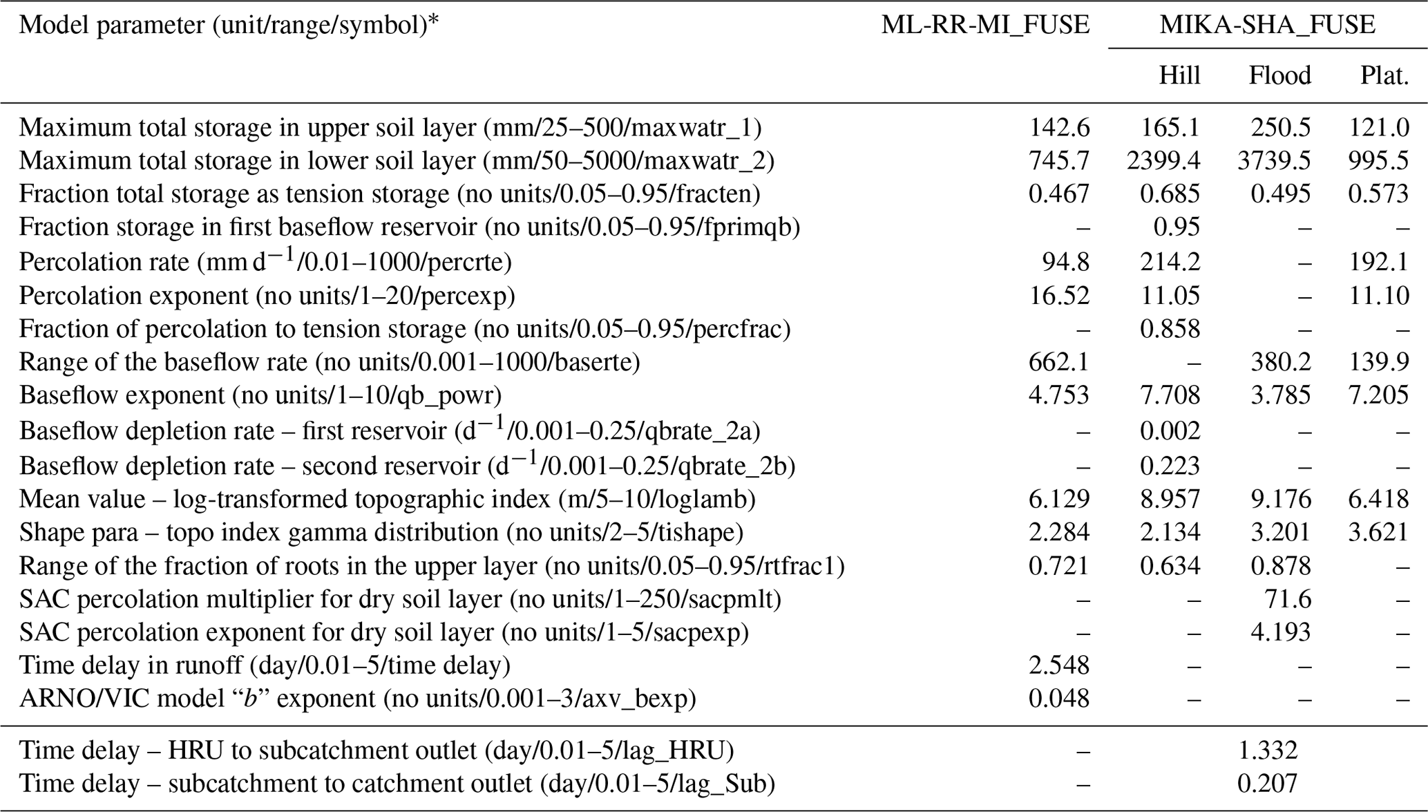
* For more details, please refer to Clark et al. (2008, 2011).
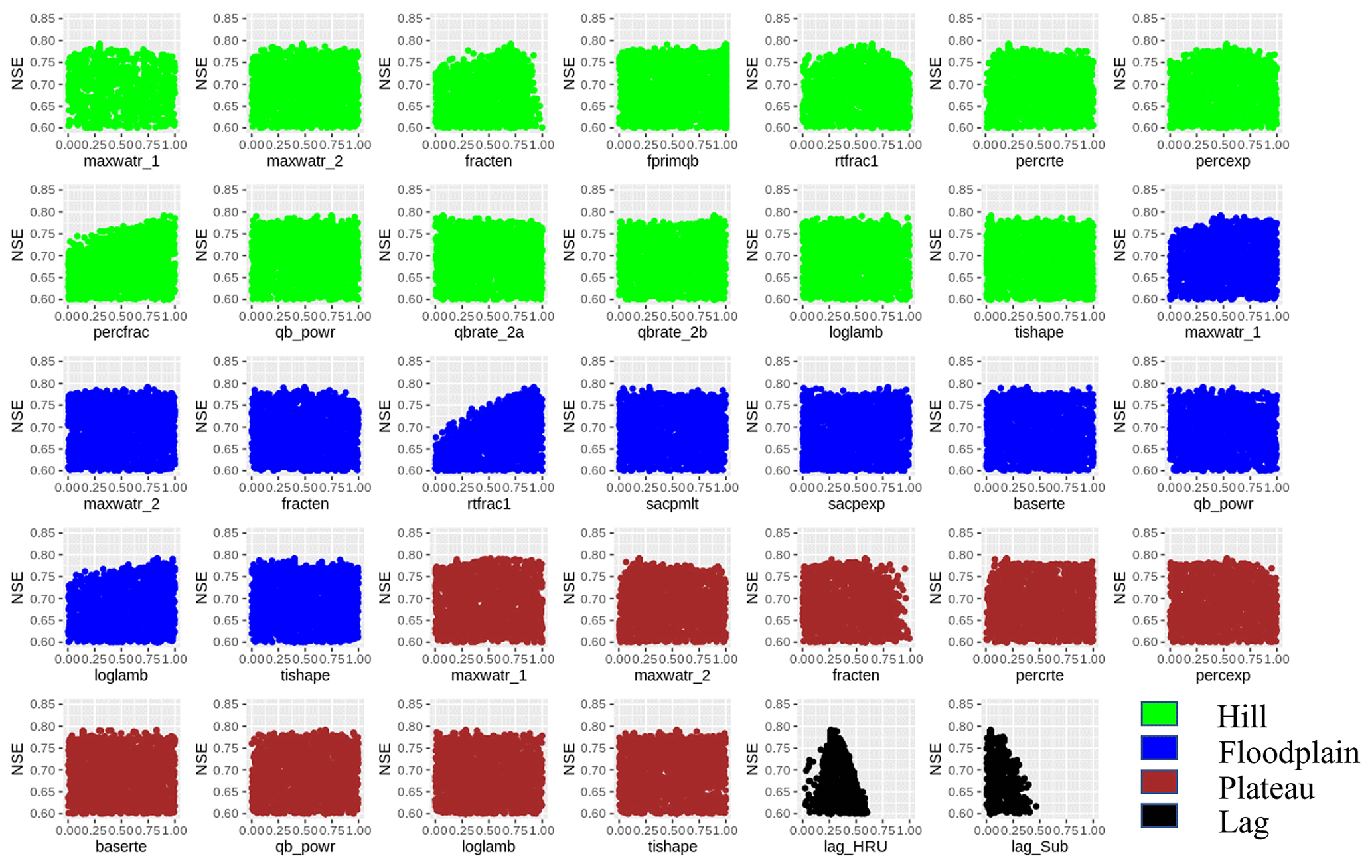
The following are the data sets used in this study:
-
United States Geological Survey (USGS) EarthExplorer's Shuttle Radar Topography Mission (SRTM) data, available at https://earthexplorer.usgs.gov/ (last access: 20 March 2020) (USGS EarthExplorer, 2020).
-
MOPEX data set, available at https://www.nws.noaa.gov/ohd/mopex/mo_datasets.htm (last access: 12 February 2021) (USGS ID 1668000; MOPEX, 2021).
-
Daymet data set, available at https://daymet.ornl.gov/ (last access: 20 March 2020) (Daymet, 2020).
-
CAMELS data set, available at (USGS IDs 1667500 and 1664000; Newman et al., 2015).
HMVVH visualized the paper, did the formal analysis, and wrote the original draft. HMVVH, VB, and JC conceptualized the paper. HMVVH and JC prepared the methodology and software. VB led the project administration, supervised the project, and reviewed and edited the paper.
The authors declare that they have no conflict of interest.
Publisher's note: Copernicus Publications remains neutral with regard to jurisdictional claims in published maps and institutional affiliations.
We greatly appreciate the support given by Vojtech Havlicek, for the R programming. Furthermore, we acknowledge Fabrizio Fenicia, for his assistance with the SUPERFLEX framework.
This paper was edited by Fabrizio Fenicia and reviewed by four anonymous referees.
Addor, N., and Melsen, L. A.: Legacy, rather than adequacy, drives the selection of hydrological models, Water Resour. Res., 55, 378–390, https://doi.org/10.1029/2018WR022958, 2019.
ASCE Task Committee on Application of Artificial Neural Networks in Hydrology: Artificial neural networks in hydrology. II: Hydrologic applications, J. Hydrol. Eng., 5, 124–137, 2000.
Baartman, J. E., Melsen, L. A., Moore, D., and van der Ploeg, M. J.: On the complexity of model complexity: Viewpoints across the geosciences, Catena, 186, 104261, https://doi.org/10.1016/j.catena.2019.104261, 2019.
Babovic, V.: Data mining in hydrology, Hydrol. Process., 19, 1511–1515, 2005.
Babovic, V.: Introducing knowledge into learning based on genetic programming, J. Hydroinform., 11, 181–193, 2009.
Babovic, V. and Abbott, M. B.: The evolution of equations from hydraulic data Part II: Applications, J. Hydraul. Res., 35, 411–430, 1997.
Babovic, V. and Keijzer, M.: Forecasting of river discharges in the presence of chaos and noise, in: Coping with floods: Lessons learned from recent experiences, nato arw series, edited by: Marsalek, J., Kluwer, Dordrecht, 1999.
Babovic, V. and Keijzer, M.: Genetic programming as a model induction engine, J. Hydroinform., 2, 35–60, 2000.
Babovic, V. and Keijzer, M.: Rainfall runoff modelling based on genetic programming, Hydrol. Res., 33, 331–346, 2002.
Babovic, V., Keijzer, M., Aguilera, D. R., and Harrington, J.: An evolutionary approach to knowledge induction: Genetic programming in hydraulic engineering, in: Proceedings of the world water and environmental resources congress, Orlando, Florida, 64, https://doi.org/10.1061/40569(2001)64, 2001.
Babovic, V., Li, X., and Chadalawada, J.: Rainfall–Runoff Modeling Based on Genetic Programming, in: Encyclopedia of Water: Science, Technology, and Society, 5 Volume Set, edited by: Maurice, P., Wiley, New York, USA, 1081–1096, 2020.
Baptist, M. J., Babovic, V., Uthurburu, J. R., Keijzer, M., Uittenbogaard, R. E., Mynett, A., and Verwey, A.: On inducing equations for vegetation resistance, J. Hydraul. Res., 45, 435–450, 2007.
Bautu, A., and Bautu, E.: Meteorological data analysis and prediction by means of genetic programming, in: Proceedings of the 5th workshop on mathematical modeling of environmental and life sciences problems, Constanta, Romania, 5–42, 2006.
Becker, R., Koppa, A., Schulz, S., Usman, M., aus der Beek, T., and Schueth, C.: Spatially distributed model calibration of a highly managed hydrological system using remote sensing-derived et data, J. Hydrol., 577, 123944, https://doi.org/10.1016/j.jhydrol.2019.123944, 2019.
Beven, J. K. and Binley, M. A.: The future of distributed models: Model calibration and uncertainty prediction, Hydrol. Process., 6, 278–298, 1992.
Beven, K.: Down to basics: Runoff processes and the modelling process, in: Rainfall-runoff modelling: the primer, Wiley-Blackwell, West Sussex, UK, 1–22, 2012a.
Beven, K.: Beyond the Primer: Next Generation Hydrological Models, in: Rainfall-runoff modelling: the primer, Wiley-Blackwell, West Sussex, UK, 313–327, 2012b.
Beven, K.: Deep learning, hydrological processes and the uniqueness of place, Hydrol. Process., 34, 3608–3613, https://doi.org/10.1002/hyp.13805, 2020.
Beven, K. and Freer, J.: Equifinality, data assimilation, and uncertainty estimation in mechanistic modelling of complex environmental systems using the GLUE methodology, J. Hydrol., 249, 11–29, 2001.
Boyle, D. P., Gupta, H. V., Sorooshian, S., Koren, V., Zhang, Z., and Smith, M.: Toward improved streamflow forecasts: Value of semidistributed modelling, Water Resour. Res., 37, 2749–2759, https://doi.org/10.1029/2000wr000207, 2001.
Cannon, A. J. and Mckendry, I. G.: A graphical sensitivity analysis for statistical climate models: Application to indian monsoon rainfall prediction by artificial neural networks and multiple linear regression models, Int. J. Climatol., 22, 1687–1708, https://doi.org/10.1002/joc.811, 2002.
Chadalawada, J. and Babovic, V.: Review and comparison of performance indices for automatic model induction, J. Hydroinform., 21, 13–31, 2017.
Chadalawada, J., Havlicek, V., and Babovic, V.: A Genetic Programming Approach to System Identification of Rainfall-Runoff Models, Water Resour. Manage., 31, 3975–3992, https://doi.org/10.1007/s11269-017-1719-1, 2017.
Chadalawada, J., Herath, H. M. V. V., and Babovic, V.: Hydrologically informed machine learning for rainfall-runoff modeling: A genetic programming-based toolkit for automatic model induction, Water Resour. Res., 56, e2019WR026933, https://doi.org/10.1029/2019WR026933, 2020.
Clark, M. P., Slater, A. G., Rupp, D. E., Woods, R. A., Vrugt, J. A., Gupta, H. V., Wagener, T., and Hay, L. E.: Framework for Understanding Structural Errors (FUSE): A modular framework to diagnose differences between hydrological models, Water Resour. Res., 44, W00B02, https://doi.org/10.1029/2007WR006735, 2008.
Clark, M. P., Hilary, K. M., Daniel, B. G. C., Kavetski, D., and Woods, R. A.: Hydrological field data from a modeller's perspective: Part 2: Process-based evaluation of model hypotheses, Hydrol. Process., 25, 523–543, 2011.
Clark, M. P., Schaefli, B., Schymanski, S. J., Samaniego, L., Luce, C. H., Jackson, B. M., Freer, J. E., Arnold, J. R., Moore, R. D., Istanbulluoglu, E., and Ceola, S.: Improving the theoretical underpinnings of process-based hydrologic models, Water Resour. Res., 52, 2350–2365, 2016.
Criss, R. E. and Winston, W. E.: Do Nash values have value? Discussion and alternate proposals, Hydrol. Process., 22, 2723–2725, https://doi.org/10.1002/hyp.7072, 2008.
Datta, B., Prakash, O., and Sreekanth, J.: Application of Genetic Programming Models Incorporated in Optimization Models for Contaminated Groundwater Systems Management, Advances in Intelligent Systems and Computing EVOLVE – A Bridge between Probability, Set Oriented Numerics, and Evolutionary Computation V, Springer, Cham, 183–199, https://doi.org/10.1007/978-3-319-07494-8_13, 2014.
Daymet: Daily Surface weather and Climatological Summaries, available at: https://daymet.ornl.gov/, last access: 20 March 2020.
Deb, K., Pratap, A., Agarwal, S., and Meyarivan, T.: A fast and elitist multiobjective genetic algorithm: NSGA-II, IEEE T. Evol. Comput., 6, 182–197, 2002.
Delgado-Bonal, A. and Marshak, A.: Approximate Entropy and Sample Entropy: A Comprehensive Tutorial, Entropy, 21, 541, https://doi.org/10.3390/e21060541, 2019.
Elshorbagy, A. and El-Baroudy, I.: Investigating the capabilities of evolutionary data-driven techniques using the challenging estimation of soil moisture content, J. Hydroinform., 11, 237–251, 2009.
Fatichi, S., Vivoni, E. R., Ogden, F. L., Ivanov, V. Y., Mirus, B., Gochis, D., Downer, C. W., Camporese, M., Davison, J. H., Brian A. Ebel, B. A., Jones, N., Kim, J., Mascaro, G., Richard G. Niswonger, R. G., Restrepo, P., Rigon, R., Shen, C., Sulis, M., and David Tarboton, D.: An overview of current applications, challenges, and future trends in distributed process-based models in hydrology, J. Hydrol., 537, 45–60, https://doi.org/10.1016/j.jhydrol.2016.03.026, 2016.
Fenicia, F., Savenije, H. H. G., Matgen, P., and Pfister, L.: Is the groundwater reservoir linear? Learning from data in hydrological modelling, Hydrol. Earth Syst. Sci., 10, 139–150, https://doi.org/10.5194/hess-10-139-2006, 2006.
Fenicia, F., Kavetski, D., and Savenije, H. H. G.: Elements of a flexible approach for conceptual hydrological modeling: 1. Motivation and theoretical development, Water Resour. Res., 47, W11510, https://doi.org/10.1029/2010WR010174, 2011.
Fenicia, F., Kavetski, D., Savenije, H. H. G., Clark, M. P., Schoups, G., Pfister, L., and Freer, J.: Catchment properties, function, and conceptual model representation: Is there a correspondence?, Hydrol. Process., 28, 2451–2467, 2014.
Fenicia, F., Kavetski, D., Savenije, H. H., and Pfister, L.: From spatially variable streamflow to distributed hydrological models: Analysis of key modelling decisions, Water Resour. Res., 52, 954–989, https://doi.org/10.1002/2015WR017398, 2016.
Fleming, S. W.: Artificial neural network forecasting of nonlinear Markov processes, Can. J. Phys., 85, 279–294, https://doi.org/10.1139/p07-037, 2007.
Giorgino, T.: Computing and Visualizing Dynamic Time Warping Alignments in R: The dtw Package, J. Stat. Softw., 31, 1–24, 2009.
Giuliani, M., Castelletti, A., Pianosi, F., Mason, E., and Reed, P. M.: Curses, tradeoffs, and scalable management: Advancing evolutionary multiobjective direct policy search to improve water reservoir operations, J. Water Resour. Plan. Manage., 142, 4015050, https://doi.org/10.1061/(asce)wr.1943-5452.0000570, 2015.
Gupta, H. V., Kling, H., Yilmaz, K. K., and Martinez, G. F.: Decomposition of the mean squared error and NSE performance criteria: Implications for improving hydrological modelling, J. Hydrol., 377, 80–91, 2009.
Guthke, A.: Defensible model complexity: A call for data-based and goal-oriented model choice, Groundwater, 55, 646–650, 2017.
Havlicek, V., Hanel, M., Maca, P., Kuraž, M., and Pech, P.: Incorporating basic hydrological concepts into genetic programming for rainfall-runoff forecasting, Computing, 95, 363–380, 2013.
Hoge, M., Wohling, T., and Nowak, W.: A primer for model selection: The decisive role of model complexity, Water Resour. Res., 54, 1688–1715, https://doi.org/10.1002/2017WR021902, 2018.
Hsieh, W. W.: Machine learning in the environmental sciences, Cambridge University Press, Cambridge, UK, 2009.
Karimi, S., Shiri, J., Kisi, O., and Shiri, A. A.: Short-term and long-term streamflow prediction by using `wavelet-gene expression' programming approach, ISH J. Hydraul. Eng., 22, 148–162, 2016.
Karpatne, A., Atluri, G., Faghmous, J. H., Steinbach, M., Banerjee, A., Ganguly, A., Shekhar, S., Samatova, N., and Kumar, V.: Theory-guided data science: A new paradigm for scientific discovery from data, IEEE T. Knowl. Data Eng., 29, 2318–2331, https://doi.org/10.1109/TKDE.2017.2720168, 2017.
Kavetski, D. and Fenicia, F.: Elements of a flexible approach for conceptual hydrological modeling: 2. Application and experimental insights, Water Resour. Res., 47, W11511, https://doi.org/10.1029/2011WR010748, 2011.
Keijzer, M. and Babovic, V.: Declarative and preferential bias in GP-based scientific discovery, Genet. Program. Evolv. Mach., 3, 41–79, 2002.
Knoben, W. J. M., Freer, J. E., Fowler, K. J., Peel, M. C., and Woods, R. A.: Modular Assessment of Rainfall–Runoff Models Toolbox (MARRMoT) v1.2: An open-source, extendable framework providing implementations of 46 conceptual hydrologic models as continuous state-space formulations, Geosci. Model Dev., 12, 2463–2480, https://doi.org/10.5194/gmd-12-2463-2019, 2019.
Koza, J. R.: Genetic programming: on the programming of computers by means of natural selection, 1, MIT Press, Cambridge, Massachusetts, UK, 1992.
Kratzert, F., Klotz, D., Herrnegger, M., Sampson, A. K., Hochreiter, S., and Nearing, G.: Toward improved predictions in ungauged basins: Exploiting the power of machine learning, Water Resour. Res., 55, 11344–11354, https://doi.org/10.1029/2019WR026065, 2019.
Krause, P., Boyle, D. P., and Bäse, F.: Comparison of different efficiency criteria for hydrological model assessment, Adv. Geosci., 5, 89–97, https://doi.org/10.5194/adgeo-5-89-2005, 2005.
Ley, R., Hellebrand, H., Casper, M. C., and Fenicia, F.: Comparing classical performance measures with signature indices derived from flow duration curves to assess model structures as tools for catchment classification, Hydrol. Res., 47, 1–14, 2016.
Mcgovern, A., Lagerquist, R., Gagne, D. J., Jergensen, G. E., Elmore, K. L., Homeyer, C. R., and Smith, T.: Making the black box more transparent: Understanding the physical implications of machine learning, B. Am. Meteorol. Soc., 100, 2175–2199, 2019.
Mehr, A. D., Nourani, V., Kahya, E., Hrnjica, B., Sattar, A. M. A., and Yaseen, Z. M.: Genetic programming in water resources engineering: A state-of-the-art review, J. Hydrol., 566, 643–667, 2018.
Meshgi, A., Schmitter, P., Babovic, V., and Chui, T. F. M.: An empirical method for approximating stream baseflow time series using groundwater table fluctuations, J. Hydrol., 519, 1031–1041, 2014.
Meshgi, A., Schmitter, P., Chui, T. F. M., and Babovic, V.: Development of a modular streamflow model to quantify runoff contributions from different land uses in tropical urban environments using genetic programming, J. Hydrol., 525, 711–723, 2015.
Molin, M. D., Schirmer, M., Zappa, M., and Fenicia, F.: Understanding dominant controls on streamflow spatial variability to set up a semi-distributed hydrological model: The case study of the Thur catchment, Hydrol. Earth Syst. Sci., 24, 1319–1345, https://doi.org/10.5194/hess-24-1319-2020, 2020.
MOPEX: Model Parameter Estimation Experiment, available at: https://www.nws.noaa.gov/ohd/mopex/mo_datasets.htm, last access: 12 February 2021.
Nash, J. E. and Sutcliffe, J. V.: River flow forecasting through conceptual models Part I – A discussion of principles, J. Hydrol., 10, 282–290, 1970.
Nearing, G. S., Kratzert, F., Sampson, A. K., Pelissier, C. S., Klotz, D., Frame, J. M., and Gupta, H. V.: What Role Does Hydrological Science Play in the Age of Machine Learning?, Water Resour. Res., 57, e2020WR028091, https://doi.org/10.1029/2020WR028091, 2020.
Nevo, S.: The Technology Behind our Recent Improvements in Flood Forecasting, Google AI Blog, available at: https://ai.googleblog.com/2020/09/the-technology-behind-our-recent.html, last access: 3 September 2020.
Newman, A. J., Clark, M. P., Sampson, K., Wood, A., Hay, L. E., Bock, A., Viger, R. J., Blodgett, D., Brekke, L., Arnold, J. R., Hopson, T., and Duan, Q.: Development of a large-sample watershed-scale hydrometeorological data set for the contiguous USA: data set characteristics and assessment of regional variability in hydrologic model performance, Hydrol. Earth Syst. Sci., 19, 209–223, https://doi.org/10.5194/hess-19-209-2015, 2015.
Oyebode, O. K. and Adeyemo, J. A.: Genetic programming: Principles, applications and opportunities for hydrological modelling, World Academy of Science, Engineering and Technology, Int. J. Environ. Chem. Ecol. Geolog. Geophys. Eng., 8, 348–354, 2014.
Physics Informed Machine Learning Conference: Physics Informed Machine Learning Conference, 19–22 January 2016, Santa Fe, New Mexico, USA, available at: http://www.cvent.com/events/physics-informed-machine-learning/event-summary-7cd2f46ebc144bdeb6e5f4106887ea04.aspx (lass access: 11 August 2021), 2016.
QGIS.org: QGIS Geographic Information System, Open Source Geospatial Foundation Project, available at: http://qgis.org, last access: 20 March 2020.
R Core Team.: R: A language and environment for statistical computing, R Foundation for Statistical Computing, Vienna, Austria, available at: https://www.R-project.org/ (last access: 20 March 2020), 2018.
Richman, J. S. and Moorman, J. R.: Physiological time-series analysis using approximate entropy and sample entropy, Am. J. Physiol. Heart Circul. Physiol., 278, 20139–20149, https://doi.org/10.1152/ajpheart.2000.278.6.H2039, 2000.
Safari, M. J. S. and Mehr, A. D: Multigene genetic programming for sediment transport modeling in sewers at non-deposition with deposited bed condition, Int. J. Sedim. Res., 33, 262–270, https://doi.org/10.1016/j.ijsrc.2018.04.007, 2018.
Sakoe, H. and Chiba, S.: Dynamic programming algorithm optimization for spoken word recognition, IEEE T. Acoust. Speech Sig. Process., 26, 43–49, 1978.
Salvador, S. and Chan, P.: Toward accurate dynamic time warping in linear time and space, Intel. Data Anal., 11, 561–580, https://doi.org/10.3233/ida-2007-11508, 2007.
Savenije, H. H.: HESS Opinions “Topography driven conceptual modelling (FLEX-Topo)”, Hydrol. Earth Syst. Sci., 14, 2681–2692, https://doi.org/10.5194/hess-14-2681-2010, 2010.
Savic, D. and Khu, S. T.: Evolutionary computing in hydrological sciences, in: Encyclopedia of Hydrological Sciences, edited by: Anderson, M. G., Wiley, New York, USA, 331–348, 2005.
Sellars, S.: “Grand challenges” in big data and the earth sciences, B. Am. Meteorol. Soc., 99, ES95–ES98, 2018.
Selle, B. and Muttil, N.: Testing the structure of a hydrological model using genetic programming, J. Hydrol., 397, 1–9, 2011.
Shafii, M. and Tolson, B. A.: Optimizing hydrological consistency by incorporating hydrological signatures into model calibration objectives, Water Resour. Res., 51, 3796–3814, 2015.
Shen, C., Laloy, E., Elshorbagy, A., Albert, A., Bales, J., Chang, F., Ganguly, S., Hsu, K., Kifer, D., Fang, Z., Fang, K., Li, D., Li, X., and Tsai, W.: HESS Opinions: Incubating deep-learning-powered hydrologic science advances as a community, Hydrol. Earth Syst. Sci., 22, 5639–5656, https://doi.org/10.5194/hess-22-5639-2018, 2018.
Sivakumar, B. and Singh, V. P.: Hydrologic system complexity and nonlinear dynamic concepts for a catchment classification framework, Hydrol. Earth Syst. Sci., 16, 4119–4131, https://doi.org/10.5194/hess-16-4119-2012, 2012.
Snauffer, A. M., Hsieh, W. W., Cannon, A. J., and Schnorbus, M. A.: Improving gridded snow water equivalent products in British Columbia, Canada: multi-source data fusion by neural network models, The Cryosphere, 12, 891–905, https://doi.org/10.5194/tc-12-891-2018, 2018.
Solander, K. C., Bennett, K. E., Fleming, S. W., and Middleton, R. S.: Estimating hydrologic vulnerabilities to climate change using simulated historical data: A proof-of-concept for a rapid assessment algorithm in the colorado river basin, J. Hydrol.: Reg. Stud., 26, 100642, https://doi.org/10.1016/j.ejrh.2019.100642, 2019.
Spieler, D., Mai, J., Craig, J. R., Tolson, B. A., and Schutze, N.: Automatic model structure identification for conceptual hydrologic models, Water Resour. Res., 56, e2019WR027009, https://doi.org/10.1029/2019WR027009, 2020.
Sugawara, M.: Automatic calibration of the tank model/l'etalonnage automatique d'un modele a cisterne, Hydrolog. Sci. J., 24, 375–388, 1979.
Todini, E.: Hydrological catchment modelling: past, present and future, Hydrol. Earth Syst. Sci., 11, 468–482, https://doi.org/10.5194/hess-11-468-2007, 2007.
Tolson, B. A. and Shoemaker, C. A.: Dynamically dimensioned search algorithm for computationally efficient watershed model calibration, Water Resour. Res., 43, W01413, https://doi.org/10.1029/2005WR004723, 2007.
USGS EarthExplorer: U.S. Geological Survey, available at: https://earthexplorer.usgs.gov/, last access: 20 March 2020.
van Esse, W. R., Perrin, C., Booij, M. J., Augustijn, D. C. M., Fenicia, F., Kavetski, D., and Lobligeois, F.: The influence of conceptual model structure on model performance: a comparative study for 237 French catchments, Hydrol. Earth Syst. Sci., 17, 4227–4239, https://doi.org/10.5194/hess-17-4227-2013, 2013.
Vitolo, C.: Exploring data mining for hydrological modelling, PhD thesis, Department of Civil and Environmental Engineering, Imperial College, London, UK, 2015.
Wagener, T., Boyle, D. P., Lees, M. J., Wheater, H. S., Gupta, H. V., and Sorooshian, S.: A framework for development and application of hydrological models, Hydrol. Earth Syst. Sci., 5, 13–26, https://doi.org/10.5194/hess-5-13-2001, 2001.
Wainwright, J. and Mulligan, M.: Environmental Modelling: Finding Simplicity in Complexity, 2d Edn., John Wiley & Sons, West Sussex, UK, https://doi.org/10.1002/9781118351475, 2013.
Wood, E. F., Roundy, J. K., Troy, T. J., Van Beek, L., Bierkens, M. F., Blyth, E., de Roo, A., Döll, P., Ek, M., Famiglietti, J., Gochis, D., van de Giesen, N., Houser, P., Jaffé, P. R., Kollet, S., Lehner, B., Lettenmaier, D. P., Peters-Lidard, C., Sivapalan, M., Sheffield, J., Wade, A., and Whitehead, P.: Hyperresolution global land surface modeling: Meeting a grand challenge for monitoring earth's terrestrial water, Water Resour. Res., 47, W05301, https://doi.org/10.1029/2010WR010090, 2011.
Xiang, Z. and Demir, I.: Distributed long-term hourly streamflow predictions using deep learning – A case study for State of Iowa, Environ. Model. Softw., 133, 104761, https://doi.org/10.31223/osf.io/vs4x8, 2020.
Yaseen, Z. M., El-shafie, A., Jaafar, O., and Afan, H. A.: Artificial intelligence based models for stream-flow forecasting: 2000–2015, J. Hydrol., 530, 829–844, https://doi.org/10.1016/j.jhydrol.2015.10.038, 2015.
Zhao, R. J.: The Xinanjiang model applied in China, J. Hydrol., 135, 371–381, https://doi.org/10.1016/0022-1694(92)90096-E, 1992.