Streamflow estimation at partially gaged sites using multiple-dependence conditions via vine copulas

Reliable estimates of missing streamflow values are relevant for water resource planning and management. This study proposes a multiple-dependence condition model via vine copulas for the purpose of estimating streamflow at partially gaged sites. The proposed model is attractive in modeling the high-dimensional joint distribution by building a hierarchy of conditional bivariate copulas when provided a complex streamflow gage network. The usefulness of the proposed model is firstly highlighted using a synthetic streamflow scenario. In this analysis, the bivariate copula model and a variant of the vine copulas are also employed to show the ability of the multiple-dependence structure adopted in the proposed model. Furthermore, the evaluations are extended to a case study of 54 gages located within the Yadkin–Pee Dee River basin in the eastern USA. Both results inform that the proposed model is better suited for infilling missing values. To be specific, the proposed multiple-dependence model shows the improvement of 9.2 % on average compared to the bivariate model from the historical case study. The performance of the vine copula is further compared with six other infilling approaches to confirm its applicability. Results demonstrate that the proposed model produces more reliable streamflow estimates than the other approaches. In particular, when applied to partially gaged sites with sufficient available data, the proposed model clearly outperforms the other models. Even though the model is illustrated by a specific case, it can be extended to other regions with diverse hydro-climatological variables for the objective of infilling.

1 Introduction

Hydrological observation records covering long-term periods are instrumental in water resources planning and management, including the design of flood defense systems and irrigation water management (Aissia et al., 2017; Beguería et al., 2019). However, available streamflow data are often limited due to several situations like equipment failures, budgetary cuts, and natural hazards (Kalteh and Hjorth, 2009). Missing data are particularly observed in remote catchments where equipment failures are repaired only after significant delays following extreme events, which can be crucial for hydrological frequency analysis. Hence, hydrologists often rely on simulated sequences to infill missing data in partially gaged catchments (Booker and Snelder, 2012) by using two primary modeling approaches, such as (1) process-based models (i.e., estimating streamflow based on a conceptual understanding of hydrological processes) and (2) transfer-based statistical models (i.e., transferring information from gaged to ungaged catchments; Farmer and Vogel, 2016). This paper focuses on the latter, which estimates historical daily streamflow at inadequately and partially gaged sites by the means of a statistical relationship.

Over the past few decades, a variety of statistical models, including simple drainage area scaling (Croley and Hartmann, 1986), the spatial interpolation technique (Pugliese et al., 2014), a regression model (Beauchamp et al., 1989), and flow duration curves (FDCs; Hughes and Smakhtin, 1996), have been developed. In particular, the flow duration curve method has been regarded as one of the most trustworthy regionalization approaches (Archfield and Vogel, 2010; Boscarello et al., 2016; Castellarin et al., 2004; Li et al., 2010; Mendicino and Senatore, 2013). If the target watershed is completely gaged, FDCs can be established using regression models to regionalize the parameter sets of defined distributions (e.g., Ahn and Palmer, 2016a; Blum et al., 2017) or to regionalize a set of primary quantiles (Cunderlik and Ouarda, 2006; Schnier and Cai, 2014; Zaman et al., 2012). On the other hand, if target watershed is poorly or partially gaged, FDC models are built using the following four steps: (1) estimating the non-exceedance probability for recorded streamflow from the target watershed of interest, (2) selecting one or multiple donor watersheds for the target watershed, (3) transferring the time series of the non-exceedance probability from the donor watersheds for missing streamflow values, and (4) converting corresponding streamflow values back from the transferred non-exceedance probability. When FDCs are utilized for partially gaged watersheds, how the donor watersheds are selected (step 2) and how the probabilities are transferred from the donor watersheds (step 3) are fairly crucial in the FDC framework.

Many studies have developed diverse approaches for steps 2 and 3 in FDC modeling. While the basic formulation is that non-exceedance probabilities of the target site are transferred by those at the single donor site, a weighted average of non-exceedance probability from the selected donor sites has been suggested by Smakhtin (1999) instead. In addition, Farmer (2015) applied a kriging model to regionalized daily standard (i.e., z scored) probabilities based on non-exceedance probabilities from many donors in a region, using the quantile function of a standard normal distribution. Although these studies are promising, the joint distribution of non-exceedance probability between the target and donor watersheds is modeled based on a Gaussian assumption, which cannot properly permit different percentile values, such as extremes that have different spatial dependence structures from donor sites. To circumvent this limitation, Worland et al. (2019) suggested the copula theory after showing that a unifying framework of copulas is equivalent to that of FDC (i.e., estimations of the conditional probabilities at the target watershed given known values at the donors).

Increasing attention has been received for copulas in the field of hydrology, with applications in flood frequency analysis, drought risk analysis, and multi-site streamflow generations (Ahn and Palmer, 2016b; Ariff et al., 2012; Chen et al., 2015; Daneshkhah et al., 2016; Fu and Butler, 2014). Copulas are effective mathematical functions that are capable of combining univariate marginal distribution functions of random variables into their joint cumulative distribution function and allow the representation of diverse dependence structures between these random variables corresponding to their family members (Sklar, 1959). For example, Fu and Butler (2014) showed that the Gumbel copula performs well in representing multiple flooding characteristics as compared to the other copulas from the Archimedean family, namely the Clayton and Frank copulas. To estimate streamflow (i.e., infilling missing data) at poorly and partially gaged sites, Worland et al. (2019) have developed bivariate copulas with an Archimedean copula but limited their application to a single donor. Despite the limitation, their bivariate copulas may be acceptable since the higher dimension of copulas is not rich enough to model all possible mutual dependencies among multi-site donors (see Karmakar and Simonovic, 2009, for details). Hao and Singh (2013) also describe that multivariate copulas are incapable of modeling multi-site data exhibiting complex patterns of dependence.

However, if the theoretical limitation of a multivariate copula is mitigated, dependency information from multiple donor sites may allow more reliable predictions of regionalized streamflow. Vine copulas, also known as pair copulas, offer a far more efficient way to construct a higher-dimensional dependence (Bedford and Cooke, 2002; Joe, 2014). They have hierarchical structures that sequentially apply bivariate copulas as the local building blocks for constructing a higher-dimensional copula. The high flexibility of vine copulas enables the modeling of a wide range of complex data dependencies. In particular, Aas et al. (2009) have popularized two classes of vine copulas, namely canonical vines (C-vines) and drawable vines (Dvines), by allowing diverse pair copula families, such as the bivariate Student t copula and bivariate Clayton copula. After a seminal paper, those two vines have been used in many fields, including economics (Arreola Hernandez et al., 2017; Zimmer, 2015), finance (Dissmann et al., 2013; Lu, 2013) and engineering (Bhatti and Do, 2019; Erhardt et al., 2015; Xu et al., 2017). Similarly, a few studies have used vine copulas in hydrologic applications with diverse purposes (Daneshkhah et al., 2016; Liu et al., 2015; Vernieuwe et al., 2015; Shafaei et al., 2017), although they have not been introduced to infill missing data.

Based on the usefulness of vine copulas, Kraus and Czado (2017) have developed a promising algorithm that sequentially fits such a Dvine copula model (M_Kraus). The algorithm adds covariates to the model with the objective of maximizing a conditional likelihood and stops adding covariates to the model when none of the remaining covariates can significantly increase the model's conditional likelihood. While it is promising, one challenge that can arise, but has not been previously discussed, is overfitting when covariates are correlated with each other. In this situation, the model may adopt ineffective covariates, and this eventually leads to poor predictions. In particular, for the purpose of infilling, streamflow values at the target site are often correlated by those of many donors. Although the structure of M_Kraus is potentially favorable to estimate streamflow, a modified model procedure is required to determine the most influential covariates.

This study forwards two novel contributions to infill missing data in the field of hydrology, i.e., (1) a Dvine copula-based model is introduced to estimate streamflow for poorly and partially gaged watersheds, and (2) the existing model (M_Kraus) is further improved by incorporating a new procedure to determine the optimal number of donor sites (namely M_Dvine). First, synthetic data are generated to compare M_Kraus and M_Dvine. In this analysis, bivariate copulas (namely M_Bicop) are also employed to demonstrate the usefulness of a high-dimensional joint dependence structure. Afterwards, a real infilling example is utilized to compare the proposed vine-based model with six other streamflow transfer models adopted in the literature.

2 Methodology

2.1 Dvine copulas

A copula C is a k-variate cumulative distribution function on [0,1]^k, with all uniform margins. The C can be understood as a function that links the marginal cumulative distributions (F₁, …, F_k) to form a joint distribution F. The C associated with joint distribution F is a distribution function $C:[\mathrm{0},\mathrm{1}{]}^k\to [\mathrm{0},\mathrm{1}]$, such that, for all streamflow vectors, q=(q₁, …, q_k)^T, C satisfies the following:

$$\begin{array}{}\text{(1)}& F\left(q_{\mathrm{1}},\mathrm{\dots },q_k\right)=C\left(F_{\mathrm{1}}\left(q_{\mathrm{1}}\right),\mathrm{\dots },F_k\left(q_k\right)\right),\end{array}$$

where C is unique if F₁, …, F_k are continuous.

Based on Sklar's (1959) theorem, a multivariate distribution function is a composition of a set of marginal distributions; thus, Eq. (1) can be expressed in terms of densities, as follows:

$$\begin{array}{}\text{(2)}& f\left(q_{\mathrm{1}},\mathrm{\dots },q_k\right)=\left[\prod _{i=\mathrm{1}}^k{f}_i\left(q_i\right)\right]c\left(F_{\mathrm{1}}\left(q_{\mathrm{1}}\right),\mathrm{\dots },F_k\left(q_k\right)\right),\end{array}$$

where c is a k-dimensional copula density acquired by partial differentiation of the copula C (i.e., c(F₁(q₁), …, $F_k\left(q_k\right)):=\frac{{\partial }^k}{{\partial }_{\mathrm{1}}\mathrm{\cdots }{\partial }_k}C(F_{\mathrm{1}}\left(q_{\mathrm{1}}\right)$, …, F_k(q_k))), and f_i(⋅) is the marginal density corresponding to F_i(⋅).

Following Bedford and Cooke (2001), any copula density c(F₁(q₁), …, F_k(q_k)) can be decomposed into a product of $k(k-\mathrm{1})/\mathrm{2}$ pair copula densities. Aas et al. (2009) adopted this idea and introduced the copula class of pair copula constructions (PCCs) known as vine copulas. These copulas are suitable for modeling various dependency structures. Vine structures established by $k(k-\mathrm{1})/\mathrm{2}$ pair copulas are arranged in k−1 trees (Brechmann et al., 2013) and can be categorized as C-vines and Dvines (Liu et al., 2015). This study focuses on Dvines since they are more widely used in practice (Daneshkhah et al., 2016).

A Dvine is characterized by the ordering of its variables (see Fig. 1). In the first tree, the dependence of the first and second variables, of the second and third, and of the third and fourth, and so on, is modeled using pair copulas. In the second tree, the conditional dependence of the first and third, given the second variable (i.e., $c_{\mathrm{1},\mathrm{3}|\mathrm{2}}\left(F\right(q_{\mathrm{1}}\left|q_{\mathrm{2}}\right)$, F(q₃|q₂))), and the second and fourth, given the third (i.e., $c_{\mathrm{2},\mathrm{4}|\mathrm{3}}\left(F\right(q_{\mathrm{2}}\left|q_{\mathrm{3}}\right)$, F(q₄|q₃))), and so on, is modeled. Similarly, the pairwise dependencies of two variables are modeled in subsequent trees conditioned on those variables which lie between the two variables in the first tree (e.g., $c_{\mathrm{1},\mathrm{5}|\mathrm{2},\mathrm{3},\mathrm{4}}\left(F\right(q_{\mathrm{1}}|q_{\mathrm{2}},q_{\mathrm{3}},q_{\mathrm{4}})$, $F\left(q_{\mathrm{5}}\right|q_{\mathrm{2}},q_{\mathrm{3}},q_{\mathrm{4}}\left)\right)$). The density of the k-dimensional Dvine can be computed as follows (Aas et al., 2009):

$$\begin{array}{}\text{(3)}& \begin{array}{rl}f\left(q_{\mathrm{1}},\mathrm{\dots },q_k\right)=& \left[\prod _{i=\mathrm{1}}^k{f}_i\left(q_i\right)\right]\times \prod _{j=\mathrm{1}}^{k-\mathrm{1}}\prod _{j=\mathrm{1}}^{k-j}{c}_{j,j+j\left|\right(j+\mathrm{1}):(j+j-\mathrm{1})}\\ & \left(F\left(q_j|q_{j+\mathrm{1}},\mathrm{\dots },q_{j+j-\mathrm{1}}\right),\right.\\ & \left.F\left(q_{j+j}|q_{j+\mathrm{1}},\mathrm{\dots },q_{j+j-\mathrm{1}}\right)\right),\end{array}\end{array}$$

where $c_{j,j+j\left|\right(j+\mathrm{1}):(j+j-\mathrm{1})}$ indicates the bivariate copula densities.

Figure 1 Example of Dvine structures with five variables, four trees, and 10 edges.

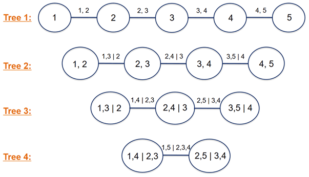
For the 5-dimensional Dvine copula, as an example in Fig. 1, the corresponding vine distribution has the following joint density:

$$\begin{array}{}\text{(4)}& \begin{array}{rl}f\left(q_{\mathrm{1}},\mathrm{\dots },q_{\mathrm{5}}\right)=& \left[\prod _{i=\mathrm{1}}^{\mathrm{5}}{f}_i\left(q_i\right)\right]c_{\mathrm{12}}\cdot c_{\mathrm{23}}\cdot c_{\mathrm{34}}\cdot c_{\mathrm{45}}\cdot c_{\mathrm{13}|\mathrm{2}}\\ & \cdot c_{\mathrm{24}|\mathrm{3}}\cdot c_{\mathrm{24}|\mathrm{3}}\cdot c_{\mathrm{35}|\mathrm{4}}\cdot c_{\mathrm{14}|\mathrm{23}}\cdot c_{\mathrm{25}|\mathrm{34}}\cdot c_{\mathrm{15}|\mathrm{234}},\end{array}\end{array}$$

where c_1,2(F₁(q₁)F₂(q₂)) is simply denoted as c_1,2.

As presented in Eq. (4), the conditional distribution functions and conditional bivariate copulas are required in vine copula modeling. The conditional distribution functions $F\left(q_j\right|q_{j+\mathrm{1}}$, …, $q_{j+j-\mathrm{1}})$, also known as h functions, in Eq. (4) can be addressed using the pair copulas from lower trees by using Eq. (5). Let q_i be a conditional value of q_j+1, …, $q_{j+j-\mathrm{1}}$, and $\mathit{\upsilon }=\mathit{\{}{q}_{j+\mathrm{1}}$, …, $q_{j+j-\mathrm{1}}{q}_i$ is the streamflow vector without q_i used in the following recursive relationship (Aas et al., 2009):

$$\begin{array}{}\text{(5)}& h\left(q_j\right|\mathit{\upsilon }):=F\left(q_j|\mathit{\upsilon }\right)={\displaystyle \frac{\partial C_{ji|\mathit{\upsilon }}\left(F\left(q_j|\mathit{\upsilon }\right),F\left(q_i|\mathit{\upsilon }\right)\right)}{\partial F\left(q_i|\mathit{\upsilon }\right)}},\end{array}$$

where the h function is associated with the pair copula C_ji|υ.

More details about Dvines can be found in Bedford and Cooke (2002) and Czado (2010, 2019).

2.2 Algorithm of the Dvine copula-based estimation (M_Dvine)

Following Kraus and Czado (2017), a two-step estimation procedure is utilized for the prediction of the streamflow value at the target watershed. The algorithm (M_Dvine) is developed using two library packages in the R programming language (Bevacqua, 2017; Schepsmeier et al., 2015).

Let q_k be the quantile of streamflow at the target watershed given the streamflow values q₁, …, q_k−1 from the donor sites. In the first step, the marginal cumulative probabilities F_k(q_k) and F_j(q_j), j=1, …, k−1, are estimated using the semiparametric approach. To be specific, this study uses the continuous kernel smoothing estimator (Geenens, 2014), which is, given the observed streamflow $q_i^{\mathit{\zeta }}$, ζ=1, …, ξ at the ith site, defined as $\widehat{F_i}\left(q_i\right)=\frac{\mathrm{1}}{nh}\sum _{\mathit{\zeta }=\mathrm{1}}^{\mathit{\xi }}\mathrm{\Omega }\left(\frac{q_i-q_i^{\mathit{\zeta }}}{h}\right)$. Here, Ω(q_i) is the kernel function, with ω(⋅) being a symmetric probability density function, and h is the parameter controlling the smoothness of the final estimate. In this study, a Gaussian kernel is used for all ω(⋅). The estimated cumulative probabilities are then employed to model the Dvine copula in the second step.

Next, to easily estimate conditional streamflow values at the target site, the Dvine copula is fitted with the fixed order $F_k\left(q_k\right)-F_{{\mathrm{I}}_{\mathrm{1}}}\left(q_{{\mathrm{I}}_{\mathrm{1}}}\right)-F_{{\mathrm{I}}_{\mathrm{2}}}\left(q_{{\mathrm{I}}_{\mathrm{2}}}\right)-\mathrm{\dots }-F_{{\mathrm{I}}_{k-\mathrm{1}}}\left(q_{{\mathrm{I}}_{k-\mathrm{1}}}\right)$, such that F_k(q_k) is the first node in the first tree, and the other orders of donors (I₁, …, I_k−1) are decided based on their correlations to the target site (i.e., $F_{{\mathrm{I}}_{\mathrm{1}}}\left(q_{{\mathrm{I}}_{\mathrm{1}}}\right)$ and showing the greatest correlations to F_k(q_k)). To build the Dvine copula model, five bivariate copulas (Gaussian, Student t, Frank, Gumbel, and Clayton) are considered as potential pair copulas (building blocks), although more families of Copulas, such as extreme value copulas (EVCs), are desirable. The five candidates may be sufficient to represent diverse dependence structures. For example, a Gaussian copula is proper when the non-exceedance probabilities between two watersheds are associated in the body of their distribution but are not asymptotically dependent in the both tails. On the other hand, a Gumbel copula may be appropriate for the situation wherein the non-exceedance probabilities exhibit tail dependence and where high flows are connected by same rainfall events but low flows are not related (e.g., due to regulation; Salvadori and De Michele, 2004). Details of the five bivariate copulas are presented in the Supplement. Parameters for the five bivariate copulas are estimated based on Kendall rank-based correlation (ρ^τ) between sites. The optimal bivariate copula for each pair copula is determined based on the penalized likelihood function (i.e., Akaike information criterion – AIC).

The final number (χ_k) of donor sites is further optimized under a cross-validation approach. In this approach, 80 % of the regional data are employed for model fitting; the other 20 % are for testing. Again, this procedure is conducted five times, and using a different set of data for testing each time. As a measure for the model's fit, the root mean squared error (RMSE; Eq. 6) from observed streamflow at the target site is utilized.

$$\begin{array}{}\text{(6)}& {\mathrm{RMSE}}_{{\mathit{\chi }}_k}=\sqrt{{\displaystyle \frac{\mathrm{1}}{\mathit{\xi }}}\sum _{\mathit{\zeta }=\mathrm{1}}^{\mathit{\xi }}{\left(q_k-{\widehat{q}}_k^{\mathit{\chi }}\right)}^{\mathrm{2}}}.\end{array}$$

Finally, conditional streamflow values at the target site can be estimated using the inverse form of the conditional distribution function (i.e., Eq. 5). To depict the ideas, a trivariate case (i.e., χ=2) is considered here. Based on the streamflow values at the donor sites (q₂, q₃), $\widehat{q_{\mathrm{1}}}$ can be obtained using the conditional distribution function $h\left(q_{\mathrm{1}}\right|q_{\mathrm{2}},q_{\mathrm{3}})$. For some fixed probabilities ϕ (e.g., ϕ=0.1, …, 0.9), $F_{\mathrm{1}}\left(\widehat{q_{\mathrm{1}}}\right)$ is derived from $C_{\mathrm{1}|\mathrm{2},\mathrm{3}}$ using an explicit function as follows:

$$\begin{array}{}\text{(7)}& \begin{array}{rl}{C}_{\mathrm{1}|\mathrm{2},\mathrm{3}}^{-\mathrm{1}}& \left(\mathit{\varphi }|F_{\mathrm{2}}\left(q_{\mathrm{2}}\right),F_{\mathrm{3}}\left(q_{\mathrm{3}}\right)\right)=h_{\mathrm{1}|\mathrm{2}}^{-\mathrm{1}}\left(h_{\mathrm{1}|\mathrm{32}}^{-\mathrm{1}}\left(\mathit{\varphi }|h_{\mathrm{2}|\mathrm{1}}\left(F_{\mathrm{2}}\left(q_{\mathrm{2}}\right)\right.\right.\right.\\ & \left.\left.\left.|F_{\mathrm{1}}\left(q_{\mathrm{1}}\right)\right)\right)|F_{\mathrm{1}}\left(q_{\mathrm{1}}\right)\right),\end{array}\end{array}$$

where $C_{\mathrm{1}|\mathrm{2},\mathrm{3}}^{-\mathrm{1}}$ is the inverse of the copula function, given the ϕ quantile curve of the copula (Liu et al., 2015; Xu and Childs, 2013). Therefore, the ϕth copula-based conditional quantile function of streamflow at the target site can be calculated as follows:

$$\begin{array}{}\text{(8)}& \begin{array}{rl}{q}_{\mathrm{1}}& \left(\mathit{\varphi }|q_{\mathrm{2}}{q}_{\mathrm{3}}\right)=F_{\mathrm{1}}^{-\mathrm{1}}\left(C_{\mathrm{1}|\mathrm{2},\mathrm{3}}^{-\mathrm{1}}\left(\mathit{\varphi }|F_{\mathrm{2}}\left(q_{\mathrm{2}}\right),F_{\mathrm{3}}\left(q_{\mathrm{3}}\right)\right)\right)\\ & =F_{\mathrm{1}}^{-\mathrm{1}}\left(h_{\mathrm{1}|\mathrm{2}}^{-\mathrm{1}}\left(h_{\mathrm{1}|\mathrm{32}}^{-\mathrm{1}}\left(\mathit{\varphi }|h_{\mathrm{2}|\mathrm{1}}\left(F_{\mathrm{2}}\left(q_{\mathrm{2}}\right)|F_{\mathrm{1}}\left(q_{\mathrm{1}}\right)\right)\right)|F_{\mathrm{1}}\left(q_{\mathrm{1}}\right)\right)\right).\end{array}\end{array}$$

Similarly, for the k-dimensional case, the ϕth copula-based conditional quantile function can be calculated, along with streamflow, at the k−1 donor sites. To acquire an estimate at the target site, 1000 samples from uniform distribution over the interval [0, 1] are generated using Monte Carlo simulations. In this study, the mean value of these generations is regarded as the best estimate.

3 Application

This study first explores the performance of M_Dvine under a synthetic example. In this analysis, M_Bicop and M_Kraus are also employed to show the usefulness of M_Dvine. For M_Bicop, the optimal bivariate copula is selected based on the AIC, while the five bivariate copulas (Gaussian, Student t, Frank, Gumbel, and Clayton) are considered as its potential candidates. A brief description of two additional models are presented in the Supplement. After that, those three models are used for a real application to 54 stream gages located in a region of the eastern USA by estimating streamflow in partially gaged locations. Finally, seven infilling approaches (Table 1) are also utilized and evaluated in a cross-validated framework to evaluate the performance of the proposed model.

Table 1 The seven infilling approaches discussed in the study.

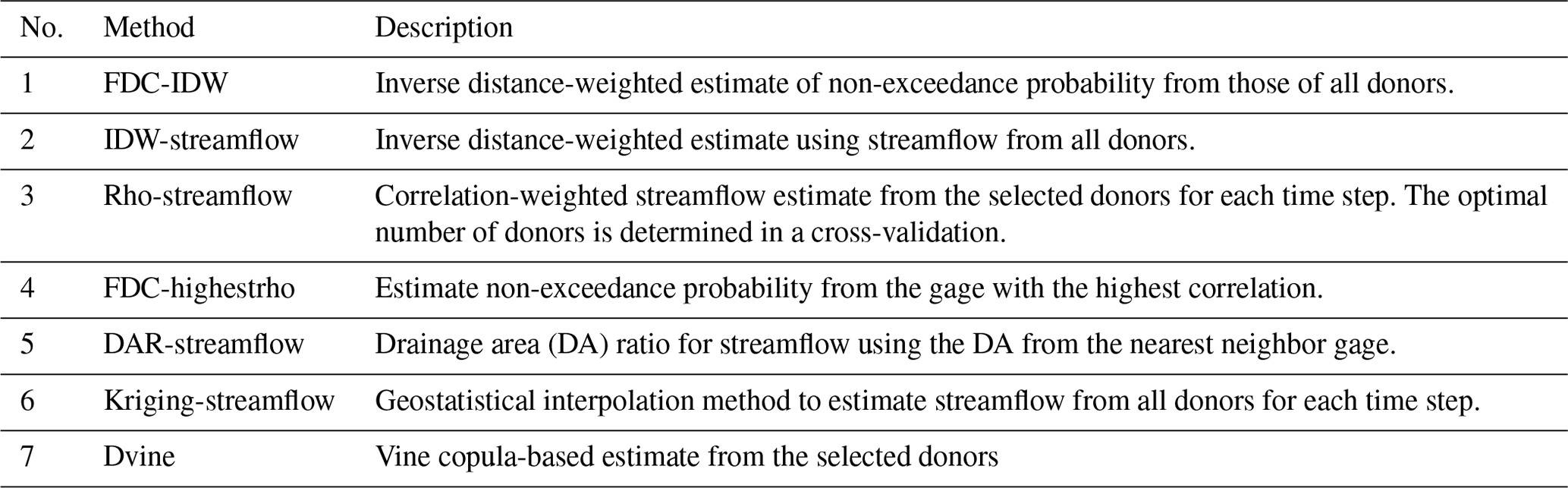
Figure 2 Structure of the 6-dimensional vine model and marginal probability function for the synthetic simulation. LN(π,σ²) denotes the log normal distribution with its mean (π) and variance (σ²). The target gage is highlighted.

3.1 Synthetic simulation

Synthetic streamflow data are generated using a controlled Monte Carlo experiment to explore how well the three copula-based models (M_Bicop, M_Kraus, and M_Dvine) provide streamflow predictions at the target site given a complex streamflow data in a pseudo gage network. In this analysis, a 6-dimensional streamflow set ($q_{\mathrm{1}}^{\mathit{\zeta }}$, $q_{\mathrm{2}}^{\mathit{\zeta }}$, $q_{\mathrm{3}}^{\mathit{\zeta }}$, $q_{\mathrm{4}}^{\mathit{\zeta }}$, $q_{\mathrm{5}}^{\mathit{\zeta }}$, and $q_{\mathrm{6}}^{\mathit{\zeta }}$), ζ=1, …, ξ=2190 (i.e. $\frac{\mathrm{2190}}{\mathrm{365}}=\mathrm{6}$ years), is modeled using four bivariate copulas (Gaussian, Student t, Flank, and Clayton) and lognormal distributions for margins (see Fig. 2).

The performance of each model is evaluated in a calibration–validation framework. First, synthetic streamflow data are generated for a 6-dimensional gage network. Then, φ years of data are randomly selected to be assumed to be known at the target gage, and the streamflow for the remaining 6−φ years of data is then estimated as missing values (φ=4 in this analysis). This process is repeated 20 times to build an ensemble prediction. In particular, this study assumes that the fifth streamflow data (i.e., q₅) will be predicted. In this assessment, two characteristics are considered to compare the three models, i.e., model prediction reliability and uncertainty quantification skill. Model prediction reliability is tested using the RMSE (Eq. 6) and Nash–Sutcliffe efficiency (NSE), which are further described in Sect. 3.4. The uncertainty quantification skill is judged by the ability of each model to build prediction intervals (PIs) that correctly bound predictions (see Sect. 3.4). Here, coverage probabilities, defined as the proportion of the time that true values occur into these PIs, are employed to show the usefulness of the proposed model.

3.2 Application to the Yadkin–Pee Dee River

The Yadkin–Pee Dee River basin (Fig. 3), covering around 18 700 km² and one of the largest river basins in North Carolina and South Carolina (Fisk, 2010), is used as real data to evaluate infilling ability. The basin flows from the northwestern corner of North Carolina near Blowing Rock and extends south by southeast, crossing the south-central border of North Carolina into South Carolina, with slightly more than half of its watershed in North Carolina. Most of the land covered within the basin is forested or used for agriculture, although urban areas in the basin are expanding.

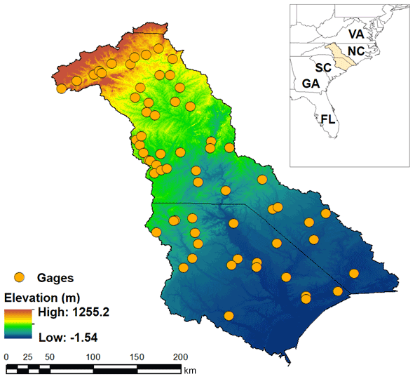
Figure 3 Map of the Yadkin–Pee Dee basin with 54 stream gage stations.

Daily streamflow data at 54 gages are gathered throughout the study region from the web interface of the US Geological Survey (USGS) National Water Information System (NWIS; US Geological Survey, 2018). The 54 gages are selected based on the following criteria: (1) all gages are recorded continuously for 15 years of daily streamflow over the period from January 2004 to December 2018, and (2) gages have non-zero daily values for the period in the first criterion, since gages with streamflow values equal to zero require a more flexible modeling structure. Thus, it is common to model zero flows separately in regionalization studies. Based on the second criterion, this study discards 10 gage stations (not shown).

3.3 Intermodel comparison framework

A set of seven infilling approaches is used in the final assessment (see Table 1), i.e., (1) M_FDC-IDW, (2) M_{IDW-streamflow}, (3) M_{Rho-streamflow}, (4) M_{FDC-highestrho}, (5) M_{DAR-streamflow}, (6) M_{Kriging-streamflow}, and (7) M_Dvine. This set of seven models is tested in a cross-validation framework under two different cases. The two cases consider situations wherein φ have values of 2 and 8 to represent relatively deficit and sufficient records for the target site. Similar to the comparative assessment to show the usefulness of the proposed copula-based model (see Sect. 3.1), each case is repeated 20 times by randomly selecting φ years over the applied period. The reliability of each model is evaluated using RMSE and NSE metrics over the validated 4-year period randomly selected in the remaining data (i.e., 4 years in 15−φ years).

3.4 Error metrics and error decomposition

As presented in Sect. 3.1 and 3.3, the RMSE (Eq. 6) and NSE are employed to evaluate prediction skills as follows:

$$\begin{array}{}\text{(9)}& \mathrm{NSE}=\mathrm{1}-{\displaystyle \frac{\sum _{\mathit{\zeta }=\mathrm{1}}^{\mathit{\xi }}{\left(\widehat{q^{\mathit{\zeta }}}-q^{\mathit{\zeta }}\right)}^{\mathrm{2}}}{\sum _{\mathit{\zeta }=\mathrm{1}}^{\mathit{\xi }}{\left(q^{\mathit{\zeta }}-\stackrel{\mathrm{‾}}{q^{\mathit{\zeta }}}\right)}^{\mathrm{2}}}}.\end{array}$$

The NSE (RMSE) can range from −∞ to 1 (0 to ∞), with higher NSE (lower RMSE) implying better performance. Both metrics have been commonly used in hydrology analysis (Boyle et al., 2000).

Following derivations suggested in Gupta et al. (2009), the RMSE can be further decomposed into three components, as follows:

$$\begin{array}{}\text{(10)}& {\mathrm{RMSE}}^{\mathrm{2}}=\mathrm{MSE}={\left(\widehat{\mathit{\mu }}-\mathit{\mu }\right)}^{\mathrm{2}}+{\left(\widehat{\mathit{\sigma }}-\mathit{\sigma }\right)}^{\mathrm{2}}+\mathrm{2}\mathit{\sigma }\widehat{\mathit{\sigma }}(\mathrm{1}-r),\end{array}$$

where $\mathit{\mu }\left(\widehat{\mathit{\mu }}\right)$ and $\mathit{\sigma }\left(\widehat{\mathit{\sigma }}\right)$ represent the average and standard deviation for the observed (estimated) streamflow, respectively, and r indicates the estimated correlation coefficient. The first component $(\widehat{\mathit{\mu }}-\mathit{\mu }{)}^{\mathrm{2}}$ is a measure of how well the average of the observed streamflow represents the average of the estimated streamflow, the second component $(\widehat{\mathit{\sigma }}-\mathit{\sigma }{)}^{\mathrm{2}}$ is a measure of how well the variance of the prediction represents the variance of the observed streamflow, and the third component $\mathrm{2}\mathit{\sigma }\widehat{\mathit{\sigma }}(\mathrm{1}-r)$ is dominated by the correlation and is defined as the timing component (Worland et al., 2019). Using these three defined components, their absolute contributions are explored in this study.

Table 2 RMSE and NSE results over the validation periods under the synthetic experiment for comparing copula-based model formulations. The best metric values for each quantile are shown in bold.

In addition, the accuracy of the uncertainty quantification skill is also evaluated for the copula-based models (M_Bicop, M_Kraus, and M_Dvine). To be specific, this study utilizes the PI coverage probability (PICP), which is a common metric for this purpose (He et al., 2017; Niemierko et al., 2019). It provides the relative number of data points that fall between the defined bounds and are expressed as follows:

$$\begin{array}{}\text{(11)}& \mathrm{PICP}={\displaystyle \frac{\mathrm{1}}{\mathit{\xi }}}\sum _{\mathit{\zeta }=\mathrm{1}}^{\mathit{\xi }}{\mathrm{\Theta }}_{\mathit{\zeta }}\mathrm{with}{\mathrm{\Theta }}_{\mathit{\zeta }}=\left\{\begin{array}{cl}\mathrm{1},& \mathrm{if}{q}^{\mathit{\zeta }}\in \left[L^{\mathit{\zeta }},U^{\mathit{\zeta }}\right]\\ \mathrm{0},& \mathrm{else}\end{array}\right.,\end{array}$$

where Θ_ζ is the indicator variable if q^ζ is covered by the ζth PI defined by the lower bound L^ζ and upper bound U^ζ. This study examines the prediction accuracy of single quantiles. Therefore, the lower bound is defined as $L^{\mathit{\zeta }}=-\mathrm{\infty }$ and $U^{\mathit{\zeta }}=\widehat{q^{\mathit{\zeta },\mathit{\varpi }}}$, where ϖ is the estimated quantile at time ζ. Accordingly, the upper bound is not a constant but is reassigned. By subtracting the nominal confidence ϖ from PICP, the average coverage error (ACE) is obtained as follows:

$$\begin{array}{}\text{(12)}& \mathrm{ACE}=\mathrm{PICP}-\mathit{\varpi }.\end{array}$$

The metric clearly indicates if the predicted quantile is underestimated (ACE < 0) or overestimated (ACE > 0), while taking small values around 0 for ideal case.

4 Results

4.1 Results for synthetic experiment

Prediction results from the out-of-sample RMSE and NSE metrics are presented for the three copula-based models (M_Bicop, M_Kraus, and M_Dvine) in Table 2. The ACE scores are also described for $\mathit{\varpi }\in \mathit{\{}\mathrm{0.05},\mathrm{0.10},\mathrm{0.50},\mathrm{0.90},\mathrm{0.95}\mathit{\}}$ in Table 3. When compared to the other models, M_Bicop achieves lower RMSE values in the right tail of the RMSE distribution over the validation periods, but severely underperforms for the majority of the designed experiment, suggesting that this model formulation, relying on a single donor, leads to poor predictions. M_Kraus provides higher RMSE values for all RMSE distributions, particularly for the right tail of the RMSE distribution. The model utilizes streamflow data from all donors (i.e., five donor sites), although the first two gages (gages 1 and 2) show insignificant associations to the target site ($r_{\mathrm{1},\mathrm{5}}=\mathrm{0.11}$ and $r_{\mathrm{2},\mathrm{5}}=\mathrm{0.14}$). M_Dvine unequivocally produces the best predictions. M_Dvine adopts streamflow data from two or three donors (gages 3, 4, and 6), without utilizing streamflow data from the first two donors when a multiple-dependence structure is established, to build an ensemble prediction. It outperforms M_Bicop and M_Kraus across all validation periods, besides a few with the worst performance. Even in this case, the maximum RMSE of M_Dvine is less than the maximum RMSE of M_Kraus.

Table 3 Results of average coverage error (ACE) over the validation periods under the synthetic experiment for comparing copula-based model formulations. The best metric values for each quantile are shown in bold.

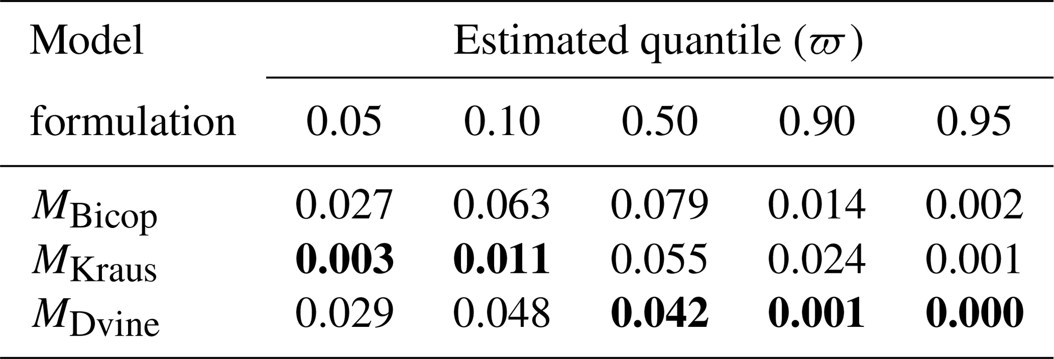
In addition, the ACE results present how the three models characterize prediction uncertainty. M_Dvine is capable of properly covering the predications across the entire distribution, while slight overestimation occurs for the smallest two quantiles. The remaining upper quantiles also tend to slightly overestimate the true values, but the overestimations are less than the other models (M_Bicop and M_Kraus). Taken together, the results of the synthetic experiment suggest that M_Dvine yields the best predictions among the copula-based models tested.

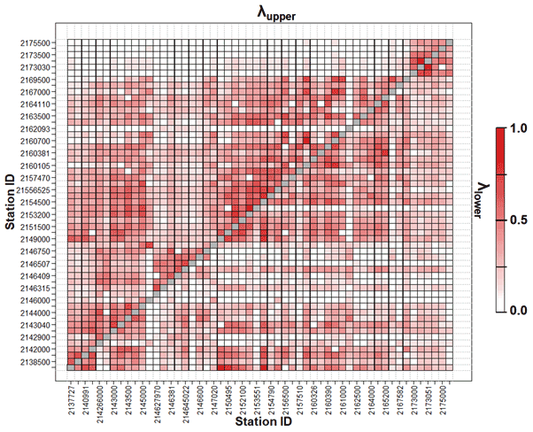
Figure 4 Pairwise upper- and lower-tail dependence for watersheds in the Yadkin–Pee Dee River basin. The upper triangular matrix shows values for the upper-tail dependence and the lower triangular matrix presents values for the lower-tail dependence. The metrics can range from 0 to 1, with higher values suggesting greater interdependence of the two streamflows for each upper- and lower tail.

4.2 Performance of the copula-based models in the Yadkin–Pee Dee River

Using the insights developed from the synthetic experiment above, the three copula-based models are applied to the streamflow data for the Yadkin–Pee Dee River. At first, upper- and lower-tail dependences (λ_upper and λ_lower) are examined for both pairs of sites (see Fig. 4), using the approach of Schmid and Schmidt (2007). The theoretical background is described in the Supplement (Sect. S3). Note that, in this analysis, the dependences become more obvious as the values approach unity. In total, two major insights emerge from this figure. First, many site pairs exhibit a strong upper-tail dependence, suggesting that streamflow variability has a tendency to be more correlated under high-flow conditions compared to low-flow conditions (i.e., asymmetric dependence). The lack of lower-tail dependence may be due to contributions governing low streamflow, such as river regulation. Next, even under high- or low-flow conditions, there is a wide range of tail dependence across the study basin (i.e., heterogeneous dependence). To sum up, a wide range of complex dependencies is observed in the streamflow data over the study basin. The complex dependences suggest that, when streamflow is estimated from multiple donors, the potential usefulness of considering a multiple-dependence structure, which is one of the main features of vine copulas, is shown.

Figure 5 shows the RMSE and NSE results for the three copula-based models under a leave-one-out cross-validation framework. This process is repeated 20 times to build an ensemble prediction by using test periods randomly defined. For this analysis, 5 years of data are selected to be assumed as the observed period at the target gage, and another 4 years are randomly selected in the remaining data for the test period. Similar to the results from the synthetic experiment, M_Kraus performs poorly in both the RMSE and NSE metrics (median of RMSE=1.549 and NSE=0.652). The bivariate copula performs well (median of RMSE=1.496), indicating that this approach efficiently leverages available information, even though the information is limited to single donor. Particularly, M_Bicop achieves the lowest RMSE values in the upper side of the RMSE box (e.g., third quartile), providing a strong uncertainty quantification skill for the upper bound. However, M_Dvine yields the best median RMSE and NSE values (=1.359 and 0.719). Given the heterogeneous dependence conditions (see Fig. 4), the high-dimensional structures are effective in modeling a complex streamflow gage network. This feature can substantially improve prediction of target site flows.

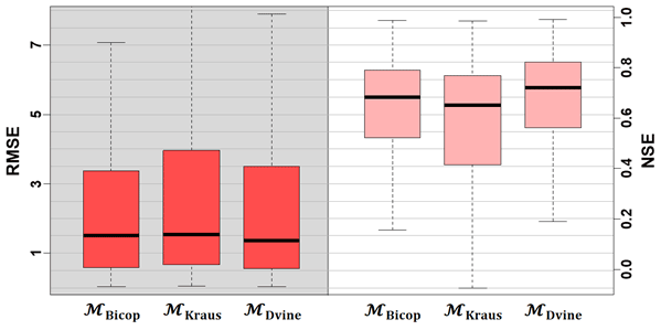
Figure 5 Model performance for the Yadkin–Pee Dee river under a cross-validation framework, based on RMSE (dark squares) and NSE (light squares). Here, the RMSE (NSE) can range from 0 to ∞ (−∞ to 1), with lower RMSE (higher NSE) implying better performance.

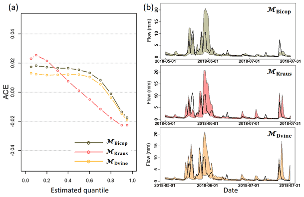
Figure 6 (a) Average coverage error from three copula-based models for the Yadkin–Pee Dee River basin across exemplary quantiles and (b) 95 % PIs for three models for an example period (1 May to 31 July 2018) for a specific target gage (USGS site ID 02143500). Observed streamflow (black solid line) is also presented in each figure.

Figure 6a presents the ACE scores described for principal quantiles, $\mathit{\varpi }\in \mathit{\{}\mathrm{0.05},\mathrm{0.10},\mathrm{0.20}$, …, 0.90,0.95}, across all target sites under the cross-validation framework. Figure 6b presents 95 % PIs for each model for an example time period (1 May to 31 July 2018) for one target site (USGS site ID 02143500). Note that the ACE would ideally take a zero value, regardless of the quantiles. The ACE scores for the three models (M_Bicop, M_Kraus, and M_Dvine) range from 0.004 to 0.0007 when considering all the quantiles together. However, the scores vary, depending on the quantiles. For instance, the ACE score for M_Kraus is noticeably positive but is almost zero around the median streamflow, indicating that the model properly represents the uncertainty of the median streamflow. M_Bicop and M_Dvine result in very similar ACE scores, although M_Dvine performs slightly better than M_Bicop. The differences in the characterization of prediction uncertainty can be confirmed from a particular target site (Fig. 6b).

Based on the results in Figs. 5 and 6, M_Dvine outperforms the other copula models (as judged by model prediction reliability and uncertainty quantification skill) and is thus selected as an appropriate copula model to infill missing data in partially gaged sites. Figure 7 shows an example application of M_Dvine, including the optimal donor sites, proper bivariate copulas, and their parameters for one target site (USGS site ID 214645022) when the model is calibrated using the full 15-year record.

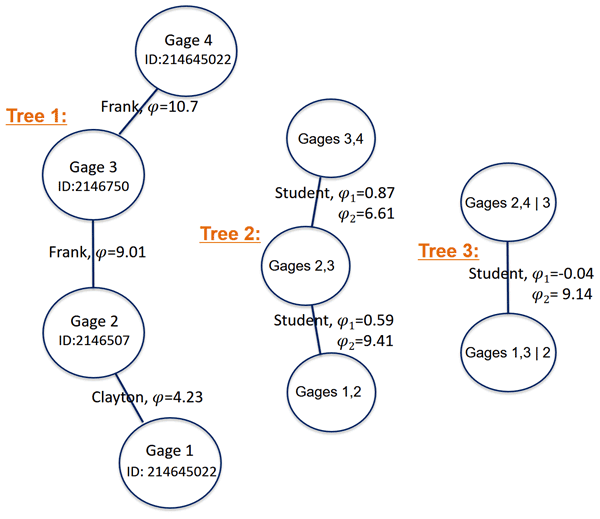
Figure 7 Structure of the Dvine copula applied for a particular target site (USGS site ID 214645022), with the defined bivariate copulas and their parameters.

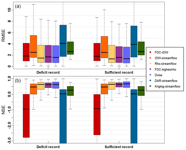
Figure 8 Intermodel comparison using cross-validation experiments based on RMSE (a) and NSE (b). Here, lower RMSE suggests more accurate estimations for infilling missing values.

4.3 Intermodel comparison for streamflow estimation

To assess the predictive skill of the proposed vine copula model, it is compared with six other statistical models (see Table 1). Figure 8 shows RMSE and NSE for the seven models where the streamflow values are estimated based on the available data defined by the two different cases, labeled “deficit record” and “sufficient record” (see Sect. 3.3). Under all cases, the vine copula approach outperforms the other infilling approaches. For example, for the sufficient record case, the median NSE for M_Dvine is 0.673, whereas those for M_{IDW-streamflow} and M_{rho-streamflow} are 0.462 and 0.649, respectively. In this analysis, the approaches, which are based on streamflow values of the donor sites without utilizing non-exceedance probability, including DAR-streamflow and Kriging-streamflow, yield relatively increased bias in their predictions. On the other hand, an application of FDC models offers reliable predictions. For instance, for the sufficient record case, the median RMSE for M_{FDC-highestrho} is 1.603 compared to that of a direct of using streamflow (e.g., median RMSE of M_{FDC-streamflow}=3.422 for the sufficient record). A similar interpretation can be found in the comparison between M_FDC-IDW and M_{IDW-streamflow}. The results from these approaches suggest that utilizing the FDC process leads to a reliable estimation, which is a primary structure in the vine copula. The other noticeable feature is that the available data length provides a significant influence on the performance of some infilling methods. In particular, this is quite evident for the vine copula model (median RMSEs are  1.598 and 1.379 for deficit and sufficient records, respectively).

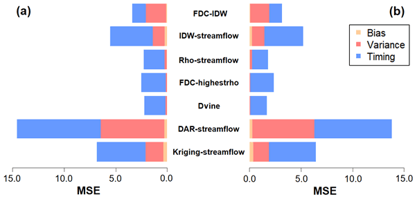
Figure 9 The three contributions from the decomposed mean squared error (MSE) for the cross-validation experiment with (a) the deficit record and (b) sufficient record scenarios.

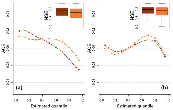
Figure 10 Average coverage error of the Dvine model for two scenarios under (a) the deficit and (b) sufficient cases. In each case, the dark line represents the scenario by the marginal cumulative probabilities using all years and conditional streamflow values constructed from the partial record. On the other hand, the light line illustrates the scenario by the marginal cumulative probabilities estimated by the partial record and conditional streamflow values constructed from the full record. The inset shows the NSE performance of the Dvine model for the two scenarios in each case.

4.4 Prediction error decomposition

The RMSE is decomposed into their components (bias, variance, and timing) for both the deficit record and sufficient record predictions (Fig. 9). For both cases, timing components primarily bring about the majority of prediction errors for all seven models. In particular, models directly estimating streamflow values (IDW-streamflow, DAR-streamflow, and Kriging-streamflow) produce a somewhat biased component, which increases when a shorter record is employed in the model. For instance, the timing component for M_{IDW-streamflow} is 4.11 and 3.75 for the deficit record and sufficient record, respectively. Moreover, timing components dominate the error metric for all cases. However, the importance of the variance component is increased, especially in three models (FDC-IDW, DAR-streamflow, and Kriging-streamflow). Lastly, the results show that, if the proposed vine copulas approach is adapted, variance and timing components are better captured, leading to better streamflow estimations, which are beneficial in the practical applications of water resources management.

Finally, the following two predictions are further produced using two additional experiments: (1) the observed marginal cumulative probabilities (i.e., using all 15 years) and conditional streamflow values constructed from the partial record (i.e., based on φ years) and (2) the estimated marginal cumulative probabilities (i.e., based on φ years) and conditional streamflow values constructed from the full record (i.e., all 15 years). Their prediction abilities are evaluated over the validated 4-year period randomly selected in the remaining data. Similar to the previous analysis, each analysis is tested 20 times. The results from these experiments provide an inference to better isolate how error components from the two-step procedure (see Sect. 2.2) influence prediction skill.

Figure 10 shows the ACE scores from the out-of-sample predictions using the proposed Dvine model under the two scenarios. When considering all the quantiles together, the ACE scores for the two scenarios are 0.003 (scenario no. 1) and 0.006 (scenario no. 2) on average under the deficit record prediction. Also, the scores under the sufficient record prediction are all nearly 0.003. Those results of the scores are sufficiently close to zero, implying that both predictions are reliable. Yet, compared to the predictions estimated by the cumulative probabilities estimated by the partial record and conditional models constructed by full records (i.e., scenario no. 2), the ACE scores are achieved better if the cumulative probabilities are determined by the full record, except for some of the low and high quantiles. Similar interpretation can be found in the NSE performance of two scenarios (see the insets in Fig. 10). It may suggest that careful attention should be paid to the first procedure (i.e., how to determine the cumulative probabilities for the target site and its donors) when M_Dvine is utilized. Nevertheless, the procedure for constructing the conditional model in a streamflow gage network is obviously crucial, since the over or underestimations are observed in many quantiles when the insufficient sampling is employed in this process.

5 Conclusion

This study introduces a multiple-dependence conditional model (i.e., vine copulas) to produce streamflow estimates at partially gaged sites. The model includes a flexible high-dimensional joint-dependence structure and conditional bivariate copula simulations. In order to confirm the usefulness of a multiple-dependence structure and the procedure for an appropriate number of donor sites in the final vine copula model, the bivariate copula model and two types of vine copulas with their unique procedure to determine the optimal number of donor sites are first investigated using the generated data. These analyses were further extended in a case study of the Yadkin–Pee Dee River basin, in the eastern USA, by estimating streamflow in partially gaged locations. In this analysis, six statistical infilling approaches were also employed to represent the applicability of the proposed model.

Results of the synthetic experiment and application to the Yadkin–Pee Dee River basin demonstrate that the propose model has benefits in some aspects. First, a multiple-dependence structure adopted in the proposed model is beneficial. From the massive evaluation experiments, this study shows that a multiple-dependence structure clearly outperforms a single-dependence structure, although there is the risk of overfitting when too many dependence structures are employed. For example, the proposed model shows the improvement of 9.2 % on average compared to the bivariate model from the evaluation experiment over the historical case study. Moreover, this study confirms that the proposed multiple-dependence structure model, with its optimum number of donor sites, produces more reliable streamflow estimation than other common infilling models. To be specific, for the sufficient record case, the proposed model shows the improvement of 13.9 % on average compared to the FDC-highestrho model. Next, the proposed model allows the development of confidence intervals to consider prediction uncertainty, which is fairly attractive compared to other models. For example, Bárdossy and Pegram (2013) argue that confidence intervals obtained using an ordinary kriging model do not reflect the prediction uncertainty well, particularly on a daily scale. Overall, this study shows that a vine copula is potentially an effective tool to support water resource management planners for objectives like gap-filling or extending missing streamflow records.

While the results of the proposed model are favorable, there are possible limitations worthy of further discussion. First, the proposed method is computationally expensive, even after adopting the multicore processing to reduce the computational burden. This becomes more problematic when the method is applied to a larger, more complex streamflow gaging network. Nevertheless, because local water managers do not need to build the model repeatedly whenever they face missing values, once the model is calibrated for a specific site, this computational burden may be a minor issue. Second, the assessment illustrated in this study focuses on model performance under cross-validation at partially gaged basins, but additional work is needed to extend the proposed model to ungaged basins; one possible way is to build a regression based model with spatial proximity and physical basin characteristics to define associations between the target and donor sites (e.g., Ahn and Steinschneider, 2019). Lastly, this study does not consider the potential nonstationarity in FDCs and correlations caused by the influence of anthropogenic activity and change in land use. Nonstationarity may not be problematic in this analysis since the assessment is limited to 15 years across the gaging network. However, if longer records were used, it would be beneficial to consider the potential nonstationarity. This exploration has been left for future work.

There are several opportunities to improve the model structure. For instance, a vine copula is able to incorporate more additional conditioning variables. One feasible approach is to add a time series of climate data (e.g., precipitation) or to decompose a time series of streamflow from the donor sites into a number of periodic components at different frequency levels through the wavelet decomposition approach (Kisi and Cimen, 2011). Moreover, although the proposed model provides a more flexible way to model multivariate dependences, it can be further improved by not adopting the standard assumption (i.e., simplifying assumption) that the conditional pair copulas depend on the conditioning variables through the conditional margins (Acar et al., 2012). One possible alternative is the use of the semi-parametric estimation of a conditional copula (Acar et al., 2012; Vatter and Chavez-Demoulin, 2015). This semi-parametric approach enables an estimate of the dependence parameters which do not rely on the simplifying assumption, eventually leading to more reliable infilling estimations. I believe that this provides an interesting avenue for future research.

Lastly, the results presented here are specific to a study basin used in a case study. The proposed model is not restricted to other watersheds around the world, and its application is further required for drawing more generalized conclusions. In addition, the model could be used for the purpose of infilling missing values of other hydro-meteorological variables besides streamflow (e.g., precipitation and soil moisture). For this application, the implementation of a vine copula with combined discrete and continuous margins (i.e., to account for no rainfall days) should be explored (e.g., Stoeber et al., 2013).