the Creative Commons Attribution 4.0 License.
the Creative Commons Attribution 4.0 License.
 | 03 Aug 2021
Taking theory to the field: streamflow generation mechanisms in an intermittent Mediterranean catchment
Karina Y. Gutierrez-Jurado
Daniel Partington
Margaret Shanafield
Streamflow dynamics for non-perennial networks remain poorly understood. The highly nonlinear unsaturated dynamics associated with the transitions between wetting and drying in non-perennial systems make modelling cumbersome. This has stifled previous modelling attempts and alludes to why there is still a knowledge gap. In this study, we first construct a conceptual model of the physical processes of streamflow generation in an intermittent river system in South Australia, based on the hypothesis that the vertical and longitudinal soil heterogeneity and topography in a basin control short term (fast flows), seasonal (slow flow), and a mixture of these two. We then construct and parameterise a fully integrated surface–subsurface hydrologic model to examine patterns and mechanisms of streamflow generation within the catchment. A set of scenarios are explored to understand the influences of topography and soil heterogeneity across the catchment. The results showed that distinct flow generation mechanisms develop in the three conceptualised areas with marked soil and topographic characteristics and suggested that capturing the order of magnitude for the average hydraulic conductivity of each soil type across the catchment was more important than pinpointing exact soil hydraulic properties. This study augments our understanding of catchment-scale streamflow generation processes, while also providing insight on the challenges of implementing physically based integrated surface–subsurface hydrological models in non-perennial stream catchments.
- Article
(7861 KB) - Full-text XML
-
Supplement
(1262 KB) - BibTeX
- EndNote


With water scarcity increasing globally, understanding the hydrology of rivers in arid and semi-arid regions has become especially important. In these regions, most streams and rivers are non-perennial, meaning surface flow ceases for some or most of the year. The understanding of the processes that lead to streamflow generation in non-perennial rivers is incomplete (Costigan et al., 2017; Gutierrez-Jurado et al., 2019; Shanafield et al., 2021). This is partly due to a lack of appropriate data; streamflow gauges are preferentially located on perennial rivers (Fekete and Vörösmarty, 2007; Poff et al., 2006). In addition, the particular challenges associated with characterising unsaturated flow and highly transient streamflow complicate the efforts to model non-perennial systems (Beven, 2002; Ye et al., 1997).
Table 1Chronology of modelling studies advancing the understanding of runoff and/or streamflow processes in non-perennial systems.
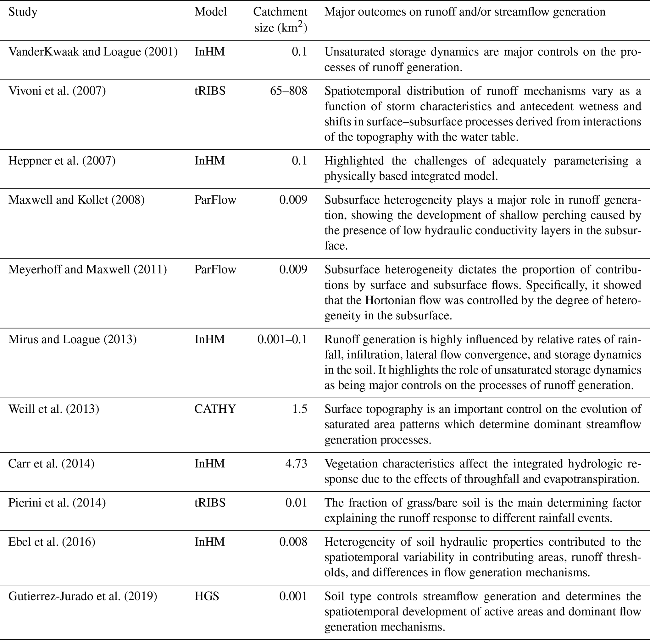
Among semi-arid regions, Mediterranean climate regions are relatively well represented in the literature because they are widespread globally, have experienced severe anthropogenic alteration, and are experiencing increasing anthropogenic water demands (Merheb et al., 2016). Intermittent rivers (i.e. those that flow seasonally) and ephemeral rivers (i.e. those that flow only after rain events) are already prevalent in these regions. Understanding streamflow generation mechanisms in these rivers is particularly needed because Mediterranean climate regions are sensitive to climate change (Cudennec et al., 2007) and are expected to experience significant drying due to shifting climate patterns, which will greatly impact streamflow regimes (Milly et al., 2005). Numerical models are used to explore the complex drivers that lead to streamflow production in a catchment. Several modelling studies of non-perennial river catchments have provided insight on the role of vegetation, soil cover, topography, antecedent wetness, and soil heterogeneity on runoff generation (Carr et al., 2014; Pierni et al., 2014; Ebel et al., 2016; Maxwell and Kollet, 2008; Vivoni et al., 2007) and on the evolution of saturated area patterns (Weill et al., 2013), as well as the importance of unsaturated storage dynamics as major controls on the processes of runoff generation (Vanderkwaak and Loague, 2001; Gutierrez-Jurado et al., 2019; Mirus and Loague, 2013; Table 1). Nevertheless, the required level of information to adequately parameterise boundary value problems has restricted the use of fully integrated surface–subsurface hydrologic models (ISSHMs) in non-perennial river catchments to mostly small-scale hillslope or headwater catchments (0.001–0.9 km2). Moreover, a majority of the numerical models for runoff and streamflow generation in non-perennial rivers investigated relatively short time periods ranging from 2 h to 330 d and reported the integrated system response to a set of scenarios (Carr et al., 2014; Di Giammarco et al., 1996; Heppner et al., 2007; Kollet et al., 2017; Mirus et al., 2009; Panday and Huyakorn, 2004). In contrast, there is still a knowledge gap regarding longer-term hydrological controls on the dry–wet transition.
The overarching, spatiotemporal processes that control key catchment-level dynamics in non-perennial rivers remains a knowledge gap. For instance, in small-scale systems, the hydrological processes occurring at a given time and place (i.e. active processes; Ambroise, 2004) might be the same as those contributing to flow generation at that same time. However, in large-scale systems the hydrologic response is influenced by different surface water–groundwater travel times, initial losses (e.g. evapotranspiration or infiltration), and the connectivity of the areas where hydrological processes are occurring. Consequently, the active processes occurring at a time and place do not necessarily contribute to the integrated catchment response at another given point at that or a later time. In contrast, a defining characteristic of the dry–wet transition in non-perennial rivers is that the dry initial conditions exacerbate initial runoff and streamflow losses due to high rates of streambed infiltration, causing the development of saturated areas and the generation of runoff and streamflow to occur discontinuously throughout the catchment.
Gutierrez-Jurado et al. (2019) used an ISSHM in an idealised concept development study to explore the processes leading to the transition from dry streambed to flowing stream. This theoretical study concluded that soil hydraulic properties and unsaturated storage dynamics exhibit strong control over streamflow generation and determine the spatiotemporal development of runoff generating areas and dominant flow generation mechanisms. It also highlighted the importance of understanding the development and progression of active areas (i.e. where processes are active) and their dominant flow generation mechanisms to understand the pathways and threshold of streamflow generation. But how applicable are the findings of this small-scale, idealised, and simplified model to real, complex, and larger-scale catchments?
We hypothesise that topography, groundwater level, and soil properties are also the dominant controls over streamflow generation mechanisms in mid-sized, Mediterranean climate coastal catchments such as those typical of South Australia. We first present a conceptual model of the potential flow mechanisms for a representative catchment, based on the theoretical findings of Gutierrez-Jurado et al. (2019), information of shallow soil profiles, and hydrological, meteorological, and geologic data. This conceptual model is then tested using an ISSHM, which is needed to fully capture the physical properties of interest. Given the inherent difficulties of modelling a large, unsaturated domain with contrasting soil layers during state changes (dry to wet), the goal of this study was not to reproduce the field observations, which in non-perennial rivers are strongly a function of antecedent moisture conditions, but to more broadly understand the interplay between shallow soil properties and groundwater levels found throughout the catchment. Finally, through simulations across the range of likely soil properties, and with varying degrees of model discretisation, we explore whether the general lack of detailed soil data at the catchment scale and computational difficulties in capturing a localised variation in stream geometry impact the characterisation of streamflow generation mechanisms.
2.1 Study area
The catchment used for this model is Pedler Creek, which is part of the larger Willunga basin located roughly 30 km south of Adelaide, South Australia (Fig. 1), in the McLaren Vale wine region. The total catchment area is approximately 107 km2 and discharges into the sea on the Gulf of St Vincent to the west of the catchment. A wastewater treatment plant located in the town of McLaren Vale discharges water into the creek; therefore, we only considered the 69 km2 area of the catchment upstream of the treatment plant (this represents 80 % of the stream network). Agriculture (45 %–30.4 km2) and grazing (46 %–31.8 km2) dominate the land use, with small urban and plantation forestry areas also dotting the catchment (Fig. 1). The creek generally flows continuously from July to September in response to the winter rains, with isolated ephemeral flows during the rest of the year after extreme rainfall events. For the (daily) period of record 2000–2018 (gauge ID A5030543; Department of Environment and Water, Government of South Australia), the creek flows on average 120 d yr−1, ranging from 33 to 199 d yr−1. Mean annual flow volume is 3.88 × 10⁶ m3, with the higher flows occurring between July and September (Water Data Services, 2019). The mean annual precipitation for the basin is 550 mm and ranges from 289 to 812 mm over the period of record (1900–2018) at the McLaren Vale station (site 232729; SILO, 2019). Mean daily temperatures range from 5 to 37 ∘C, with higher daily temperatures occurring in January and lower daily temperatures registered during June and July (SILO, 2019).

Figure 1Pedler Creek catchment location showing the original watershed boundary, the stream network, and the Willunga Fault. The five major land uses are shown for the model sub-basin.
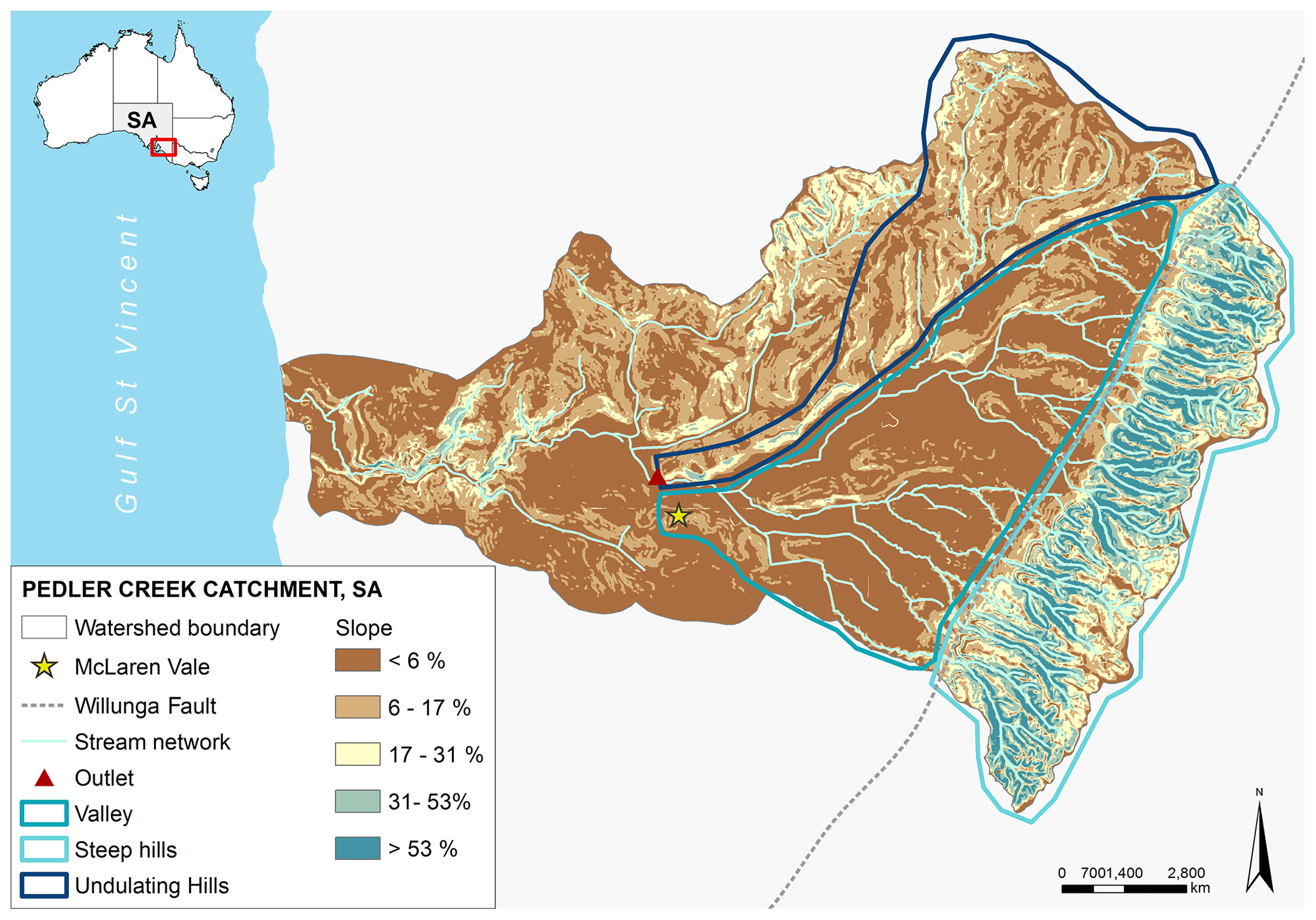
Figure 2Pedler Creek catchment slopes highlighting the three distinctive areas for the sub-catchment area, namely undulating hills in the north, the steep hills to the east, and the low gradient valley.
The catchment topography consists of a low-lying coastal plain with mild undulating hills towards the north of the catchment and separated by the Willunga Fault to the steep hills located on the east of the catchment (Fig. 2). The elevation ranges from ∼ 400 m on the northeast of the catchment (steep hills) to ∼ 50 m at the catchment's outlet. The hills area on the east of the fault is characterised by having a shallow sediment profile (0.5–2 m) which is underlain by the basement rocks, while the sediments thicken seaward west of the fault. Surficial soil types (the upper 1.5 m) in the catchment can be clustered into three major soil groups, namely loam, sand, and clay. Covering roughly 62 % (42.36 km2) of the catchment, the loam soils are distributed in the middle-eastern area where the majority (80 %) of the stream network is located. Sandy soils cover around 32 % (21.7 km2) and are located mainly in the north part of the catchment, with some patches present in the middle section (valley), while clay soils account for only 6 % (3.94 km2) of the catchment area and are located in the further downstream section towards the west of the catchment. Soil profiles consistently show a distinctive clay layer starting from 1.1 to 1.5 m depth in the sandy soil areas and at around 0.5 m within the loam areas (Department of Environment Water and Natural Resources, Government of South Australia). Below these shallow soils, regional groundwater flows from northeast to southwest towards the coast. The groundwater system consists of four main aquifers, namely Quaternary sediments, the Port Willunga formation, the Maslin Sands, and the basement fractured rocks (Aldam, 1989). The Maslin Sands and the Port Willunga aquifer are separated in some locations by the Blanche Point formation, which acts as an aquitard.
Surface water–groundwater interactions within the Pedler catchment play a critical role in the creek's flow regime. Sereda and Martin (2000) observed rapid groundwater level rises in response to large precipitation events in some shallow monitoring wells adjacent to creeks. They also noted that the groundwater (GW) level declines in the Quaternary aquifer during 1995–1999 could be attributed to a decrease in yearly precipitation during that period. Harrington (2002) observed that groundwater levels seemed to mirror streamflow records for the creek. While these observations confirm that GW recharge occurs from precipitation and creek seepage, these and other studies have also indicated that GW discharge occurs in some areas of the creek (Harrington, 2002; Anders, 2012). Further studies have indicated that the creek presents both gaining and losing stream sections, which are not only spatially but temporally variable and which are dependent on rainfall and shallow groundwater levels (Harrington, 2002; Brown, 2004; Irvine, 2016; Anders, 2012).
2.2 Conceptual model of streamflow generation process in Pedler Creek
For medium- to large-sized catchments such as Pedler Creek, the interactions between topographic features such as slope and mean soil thickness, with surficial soil heterogeneity, various aquifer properties, and a spatially variable depth to GW are likely to result in variability in streamflow generation processes developing at different spatiotemporal scales within the catchment. To understand the integrated catchment response and the stream network dynamics (development, expansion, and contraction), it is paramount to capture the spatiotemporal occurrence of the different streamflow generation mechanisms. Gutierrez-Jurado et al. (2019) identified five streamflow generation mechanisms that can occur either on the hillslope or directly in the stream, namely infiltration excess overland flow (IE-OF), saturation excess overland flow (SE-OF), interflow originating from unsaturated or saturated areas (unsat-IF and sat-IF), and pre-event groundwater (old GW). These mechanisms were therefore considered in our conceptual model.
Table 2Hydraulic mixing cell delineated fractions.

Note: HMC – hydraulic mixing cell; IF – interflow; SE-OF – saturation excess overland flow; IE-OF – infiltration excess overland flow; GW – groundwater. ∗ Common names used for the fractions are shown in parenthesis.
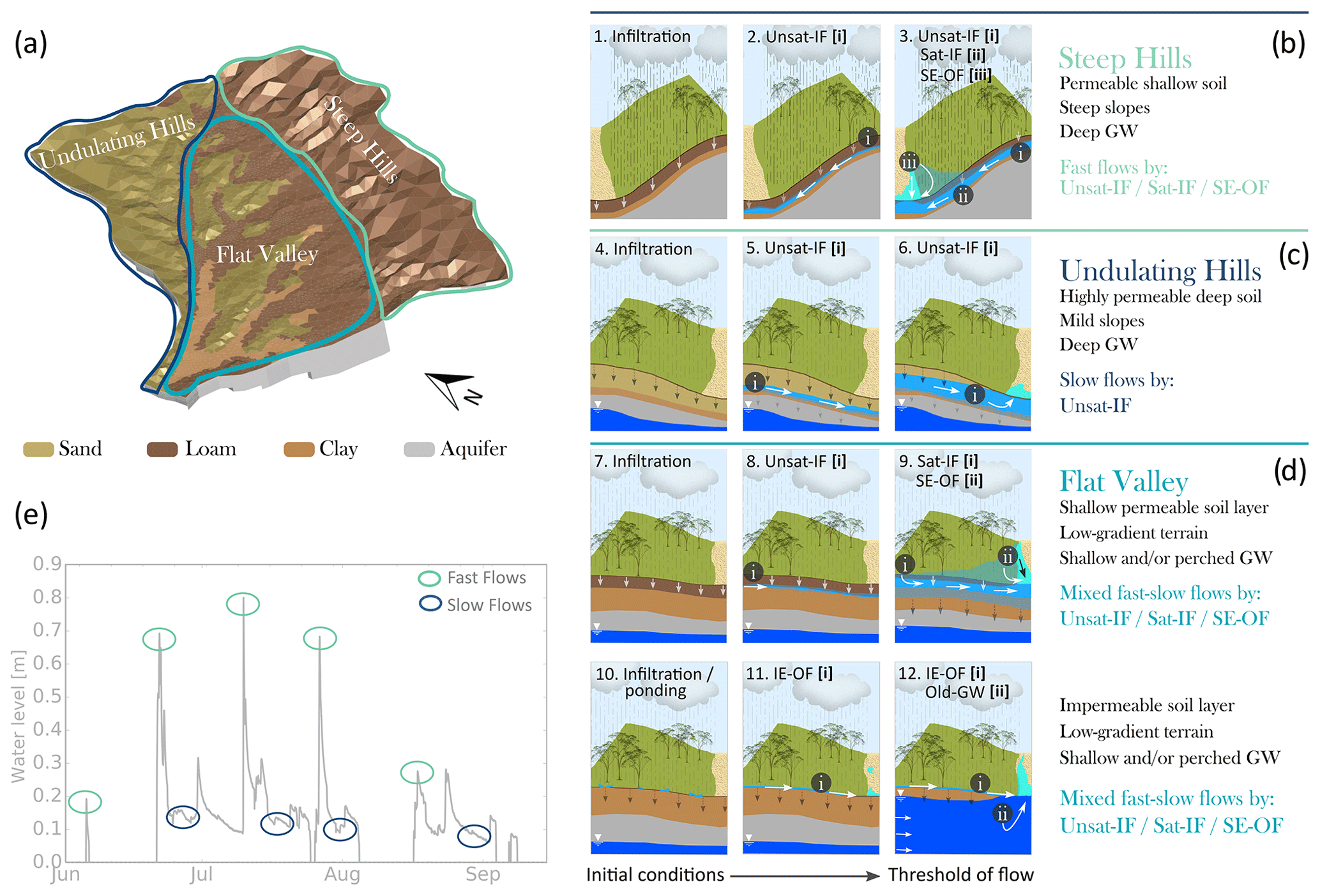
Figure 3(a) Conceptual diagram showing the three major areas that are likely to develop distinct streamflow generation mechanisms during the intermittent flow season. (b–d) The 2D soil profiles for the three major areas detailing the processes developing from the initial conditions until the threshold of flow (modified from Gutierrez-Jurado et al., 2019). (e) Typical hydrograph during the intermittent season highlighting the hypothesised fast and slow flow components. For illustration purposes, the aquifers are presented as a single unit depicted in grey. Arrows represent the flow direction.
Using available soil and topography information for the catchment (DEW, 2016; Hall et al., 2009; DEWNR, 2016), we first developed a conceptual model to outline the most likely processes leading to streamflow generation and the resulting dominant streamflow generation for Pedler Creek (Table 2). We identified the following three major areas with distinctive characteristics: (1) the steep hills to the east, (2) the undulating hills to the north, and (3) the flat valley in the southwestern area of the catchment (Fig. 3a). These three areas provide a spatial understanding of the most likely streamflow generating processes, with different processes and areas of the catchment contributing to the short ephemeral flows during summer and late fall, the early winter buildup to intermittent flow, and, throughout the rainy season, continuous flow. A detailed description of the processes for each area and the spatiotemporal development of the most likely dominant streamflow generation component for intermittent flow is provided below (Fig. 3b–d).
2.2.1 Steep hills; fast flow
The steep hills are characterised by a permeable and shallow (top 0.5 m) loam soil underlain by a heavy clay profile with steep slopes (Fig. 3b). The combination of the shallow loam soil permeability, the high infiltration capacity, and the steep slopes are likely to allow the water to infiltrate and to flow relatively fast as unsaturated IF towards the stream (Fig. 3b1–2). We hypothesise that the shallow loam soil profile and the water holding capacity of the loam will promote a perched GW mounding along the riverine area, which will result in SE-OF from the riverine area and the adjacent hillslope developing as the dominant streamflow generation mechanism (Fig. 3b3). We hypothesise that this area contributes heavily to the temporally isolated ephemeral flows and the dominant flow generation mechanism for these events would be infiltration excess overland flow.
2.2.2 Undulating hills; slow flow
The undulating hills consist of a highly permeable deep (top 1.1 m) sandy soil profile underlain by a heavy clay layer with mild slopes (Fig. 3b). We expect that the high soil infiltration capacity and permeability of the sand will result in a large infiltration rate allowing most of the early winter precipitation to infiltrate in this area (Fig. 3c4; Blasch et al., 2006; Batlle-Aguilar and Cook, 2012; Mihevc et al., 2002). As the infiltrated water reaches the low permeable clay layer, it will move in the subsurface as IF towards the low-gradient areas (Fig. 3c5). We hypothesise that the high infiltration rates in combination with the mild slopes (or low-gradient areas in the valley) will favour the development of a perched GW that will rise uniformly, allowing the river to develop into a gaining condition. As the infiltrated water moves as IF it will discharge into the downstream areas (Fig. 3c6). Due to the larger unsaturated storage and the mild slopes, this area will likely take longer to contribute to flow (i.e. more water and, therefore, more time will be needed to reach the threshold of flow generation). We hypothesise that these areas will therefore provide the slow flows necessary to sustain intermittent flow for the days without rainfall during the intermittent season, and conversely, they are not likely to contribute to flow during ephemeral events (Fig. 3e).
2.2.3 Flat valley; mixed flows
The flat valley comprises a mix of the previous two soil profiles (deep sand and shallow loam underlain by heavy clay) and a heavy clay area, all located in a low-gradient topography (Fig. 3d). The GW becomes shallower near the riverine areas in the valley and depth to GW decreases towards the outlet area (the bore with the shallowest GW is located near the outlet where the GW is ∼ 2 m below surface elevation). This zone has the largest draining area with both the steep and undulating hills draining towards it. The diversity of conditions in this area is likely to result in a combination of the processes previously discussed and additional ones. We hypothesise that the processes originating in the sandy soil areas in the valley will be similar to those on the undulating hills, with the difference that the unsaturated IF that might originate early during the season might only contribute with a small amount of flow that might reflect further downstream. We also expect to see some saturated/unsaturated IF originating early in the season in the loam areas in the valley (Fig. 3d.8–9). However, we hypothesise that the low-gradient terrain, along with the water holding capacity of the loam soil, will slow down water moving as interflow and rather promote the soil saturation to build up in the shallow soil profile. As the saturation increases, we expect the dominant streamflow generation mechanism will switch to saturation excess overland flow from both the hillslope and the river area.
The clay's low permeability will limit infiltration and favour water to pond on the surface on the clay areas, which will eventually result in infiltration excess overland flow (Fig. 3d10–11). The large draining area of the valley, combined with the low-gradient topography, is likely to promote the development of a perched GW along the riverine area, which will result in SE-OF along some sections of the river (Fig. 3d9). During wet years, sections of the creek near the outlet where GW is shallow are likely to develop into a gaining state with old GW contributing to streamflow (Fig. 3d10). Once the saturation threshold has been met along the riverine area in the steep hills and throughout the loam areas in the valley, SE-OF from those areas and the IE-OF from the clay are likely to contribute with the fast flows as travel times for overland flow are generally smaller than those for subsurface processes (Fig. 3b).
2.3 Modelling platform and HMC method
To explore the potential for streamflow within the structure of the conceptual model, we built a fully integrated, numerical model of the catchment with the hillslope fraction divided into the three dominant soil types (Fig. 4). We used HydroGeoSphere (HGS), a 3D fully integrated surface–subsurface hydrological model (ISSHM) that allows physically based simulations of hydrological processes by using the control volume finite element method to simultaneously solve the surface and subsurface flow equations. The numerical code uses the diffusion wave approximation to the Saint-Venant equations for 2D surface flow and a modified form of the Richards' equation to solve the variably saturated subsurface flow. Further details on the physical and mathematical conceptualisation and the implementation of the HGS code can be found in Aquanty (2016) and the review by Brunner and Simmons (2012).
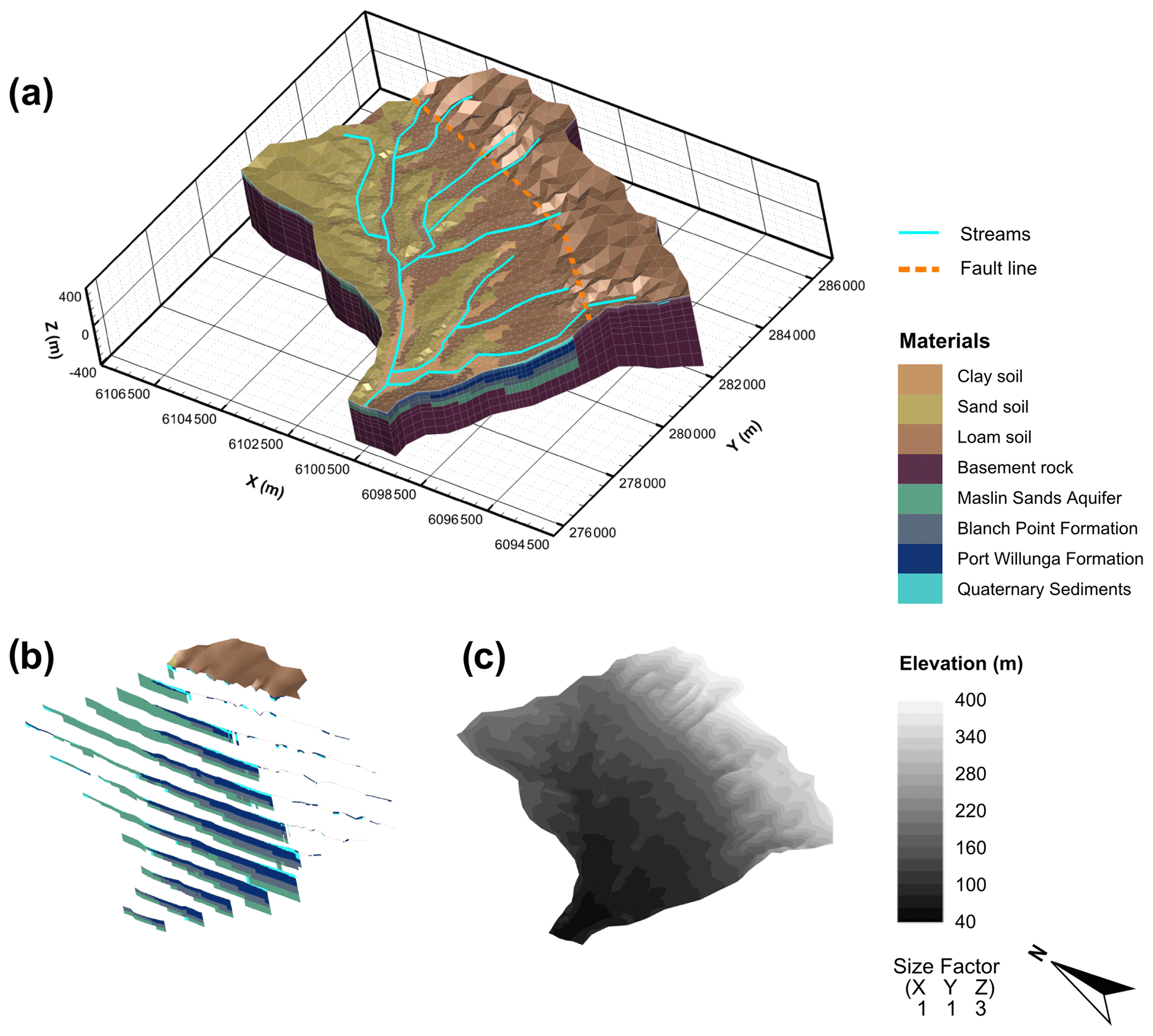
Figure 4(a) A 3D representation of the Pedler catchment showing the mesh discretisation and the spatial distribution of shallow soil types. (b) Slices showing the distribution and thickness of the hydrogeological layers. (c) Digital elevation model showing the surface topography. Approximated location of the discretised stream network and the fault line are superimposed for illustration purpose.
The decomposition of flow into the different flow generation mechanisms is provided by coupling HGS with the HMC method, which is based on the modified mixing cell method (Campana and Simpson, 1984). Using the standard hydrological output from a numerical model, the HMC method allows the partition of flow in any node within the catchment. To do this partition, the HMC method tags the existing water at the beginning of the simulation and any new water as it enters the model domain by area of origin (i.e. stream, hillslope, and the porous media) and by boundary condition (i.e. the source of water). New water is tagged by the internal model state of saturation of the area of origin (i.e. saturated or unsaturated soil profile). Using these tags, the water is tracked as it moves through the model domain, and after each time step of the flow simulation, the method calculates the fraction of water in each cell that derives from the different flow components (Table 2). Detailed information on the numerical formulation and application of the HMC method are given in Partington et al. (2011, 2013) and Gutierrez-Jurado et al. (2019).
2.4 Model setup
A three-dimensional HydroGeoSphere (HGS; Therrien et al., 2010) model of the catchment, coupled with the hydraulic mixing cell method (HMC) developed by Partington et al. (2011) was used to test the conceptual model. The HMC method tracks rainfall as it moves through the catchment, allowing the identification of active areas and the quantification of the contributing flow generation mechanisms on those areas.
2.4.1 Model discretisation
The topography for the surface elevation was implemented by using a digital elevation model (DEM) with 5 m contours and a final resolution of 10 m (Department of Environment and Water, Government of South Australia). After testing several potential nodal spacing options (see the Supplement for a description of this process), the final 2D surface domain discretisation consisted of 3015 nodes and 5869 triangles, with nodal spacing ranging from ∼ 40–70 m around the streams and up to ∼ 500 m at the catchment boundary. Vertically, the subsurface domain was discretised into 28 layers (Fig. 4). For layers 1–2 the resolution was 0.05 m, followed by 0.2 m in layers 3–13 (up to a depth of 2.1 m), grading to 5 m in layers 14–18 (a depth of 20 m), and 12 to 120 m at the bottom of the domain in layers 19–28. The final 3D grid consisted of 84 420 total nodes and 159 192 total triangular elements. As the streams in the study area were only a few metres wide, the DEM did not capture the incision of the streams into the landscape. In order to overcome this limitation, the digital elevation model was post-processed using a Python script to depress the elevation of the stream nodes.
2.4.2 Porous media properties
Hydraulic conductivity, porosity, and specific storage based on the literature estimates for the Quaternary sediments, the Port Willunga formation, the Blanche Point formation, and the Maslin Sands were assigned using rasters of the top and bottom elevations for each unit (Aldam, 1990; Anders, 2012; Irvine, 2016; Martin, 1998, 2006; Table 3). Unsaturated hydraulic parameters were then estimated from Carsel and Parrish (1988) and Mirus et al. (2011a), which had the closest hydraulic conductivity values to the estimates for each hydrogeological unit. The basement fracture rock formation is believed to act as an impervious layer throughout most of its length (Knowles et al., 2007; Martin, 1998); therefore, the elements for this layer were assumed to be inactive on the timescale of these simulations.
Table 3Surface–subsurface parameters for Pedler Creek. See Fig. 1 for land use distribution.

The shallow soils were considered as being the top 1.5 m of the subsurface domain, which was the average depth reported in the soil characterisation data sheets. The information of the horizontal and vertical distribution of soils was assigned into the model using 2D overlays (horizontal) for the three main soil areas and the mesh layers generated during the grid discretisation (vertical). We used a digital soil–landscape map (DEW, 2016; Hall et al., 2009) to differentiate the spatial distribution of the three dominant shallow soil types. The vertical heterogeneity was determined by analysing soil characterisation data sheets from detailed soil profiles available within the Pedler sub-catchment (DEWNR, 2016).
As quantitative soil hydraulic properties were not available, we tested a range of hydraulic parameters representative of the three main soil types (sand, loam, and clay) obtained from Carsel and Parrish (1988), as shown in Table 3. To validate the selected range, we estimated soil hydraulic values from six soil profiles (two within the Pedler sub-catchment and four nearby) that included data of the particle size distribution at different depths (soil layers) using the ROSETTA model H2 (Schaap et al., 2002). As explained below, the influence of the hydraulic conductivity values for each shallow soil, which is typically highly variable and not well known at the catchment scale, was then explored using scenarios.
2.4.3 Overland flow properties
Manning's roughness coefficients (n) derived from Chow (1959) were implemented for the three prevalent land uses (i.e. agricultural, pasture, and urban) which account for over 99.5 % of the catchment area. We used the values for cultivated areas with mature row crops (4.05 × 10⁻⁷ d m) for the agricultural areas and for pasture with no bush and short grass (3.47 × 10⁻⁷ d m), and the value of asphalt (1.85 × 10⁻⁷ d m) was applied to the urban area (Table 3). For the stream network, we used values for a clean and straight natural channel for the headwater sections (4.05 × 10⁻⁷ d m) and of weedy reaches for the middle lower sections (1.15 × 10⁻⁶ d m). Rill storage height was uniformly set to 0.01 m across the domain, and no obstruction storage height was implemented. The coupling length was set at 0.001 to warrant a good coupling of the surface–subsurface domains, which is paramount to capture streamflow generation processes (Liggett et al., 2014).
2.4.4 Simulation period and initial conditions
We selected a 4-year simulation period from January 2015 to December 2018 to ensure a representative set of years with average (2017 ∼ 500 mm yr−1), below average (2015 and 2018 ∼ 400 mm yr−1), and above-average (2016 ∼ 800 mm yr−1) annual rainfall amounts. Precipitation records (15 min data) from the McLaren Vale (located in the valley) and the McLaren Flat (located near the steep hills) stations (MEA, 2019) were averaged and applied as a fluid flux to the surface of the model domain. To determine the optimal time resolution for the precipitation forcing, we tested preliminary models with quarterly hour, 1 h, and 24 h inputs. Results from the preliminary models show better convergence and smaller errors in the water balance for the hourly precipitation inputs. Estimates of potential evapotranspiration (ET0) were only available at a daily time step; therefore, we used values of solar radiation to approximate ET0 at hourly intervals to match the precipitation inputs. Values of ET0 that were less than 0.0001 m h−1 were considered numerical noise and were excluded from the input data set. The resulting ET0 data set was applied to the surface domain. Actual evapotranspiration (ET) and interception are simulated as mechanistic processes within HGS, using the concepts by Kristensen and Jensen (1975) and Wigmosta et al. (1994), which require plant and soil conditions (Aquanty, 2016). Vegetation characteristics cited in the literature for eucalyptus were used on the riverine area, and values typical of grass (Banks et al., 2011; Geeroms 2009; Hingston et al., 1997) were used for the rest of the catchment (Table 3). Although a large area on the catchment consists of vineyards, during the winter months the vines are dormant without leaves, and grass is commonly used as an inter-row soil cover. We did not include the effects of irrigation, ET, and interception during the vines' growing season as we considered the overall effects for streamflow generation would be negligible since they occur during the driest and hottest months of the year when the stream network is dry. With the simulation starting in January (the hottest month), we assumed completely dry initial conditions for the surface domain (i.e. no presence of surface water).
Initial groundwater levels were achieved by draining a fully saturated model and comparing the resulting water table to field data; this process of draining required model simulations to run for days to weeks. The goal was to obtain realistic soil moisture profiles characteristic of dry summer conditions and a smoothly varying water table surface. The resulting water levels were compared with the long-term average of data obtained from the Government of South Australia (https://www.waterconnect.sa.gov.au/, last access: 18 July 2019) for the McLaren Vale prescribed wells area. Preference was given to matching wells with shallow GW heads (< 10 m depth) located on the flat valley area and close to streams, which are known to transition from losing to gaining conditions in response to increases in the groundwater level. Finally, an output time where the simulated GW heads at four of the five wells in this area were within 1 m of average recorded levels was selected as the initial conditions for the porous media in the subsequent simulations. Initial groundwater levels in the steep hills area matched average recorded levels within 1–28 m, where the depth to water is quite deep and varies by tens of metres across the fault line (Fig. 4).
2.4.5 Boundary conditions
Boundary conditions for the outflow in the surface domain were set as a critical-depth boundary at the catchment's outlet and as a no-flow boundary condition for the rest of the domain. We applied a fluid transfer boundary condition around the catchment outlet, which allows for the discharge of groundwater through the subsurface. The hydraulic gradient for the fluid transfer was given by setting a hydraulic head ∼ 4 m below the surface elevation (the known deepest GW head near the outlet) at 10 m from the outlet faces.
2.4.6 Simulation implementation and data post-processing
The simulations were performed in HGS using the control volume finite element mode and the dual node approach for surface–subsurface coupling. We used an adaptive time step with a computed under-relaxation factor scheme to aid the computational efforts. Adaptive time-stepping was applied, with an initial step size of 0.001 d, a maximum step multiplier factor of 2.0, and a maximum time step of 5 d. The simulations were run in parallel mode, using six cores from an AMD EPYC 7551 processor at 2.55 GHz (with 32 cores or 64 threads) compute node to partition the model domain. The HMC method was set up to track the flow generation mechanisms originating from the different soils in the overland areas (clay, loam, and sand), directly in the river, and from the porous media (Table 2).
We ran over 52 preliminary models testing different mesh discretisations and time resolutions for the model forcings (i.e. precipitation and ET), simulation control values, and draining simulations to try to select the optimal model setup. From the final setup, we developed a final set consisting of eight scenarios to be tested, with four corresponding to sets with different combinations for the shallow soils hydraulic properties (Ksat and their corresponding unsaturated storage parameters α, β, and θr) and four scenarios with different values for incising the river nodes (Table 4). Due to the computational constraints, only one set of soil hydraulic properties was used to test the scenarios with the incised stream. Results from these two sets of scenarios were used to evaluate the need to modify and test further scenarios.
Table 4Properties of tested model scenarios.
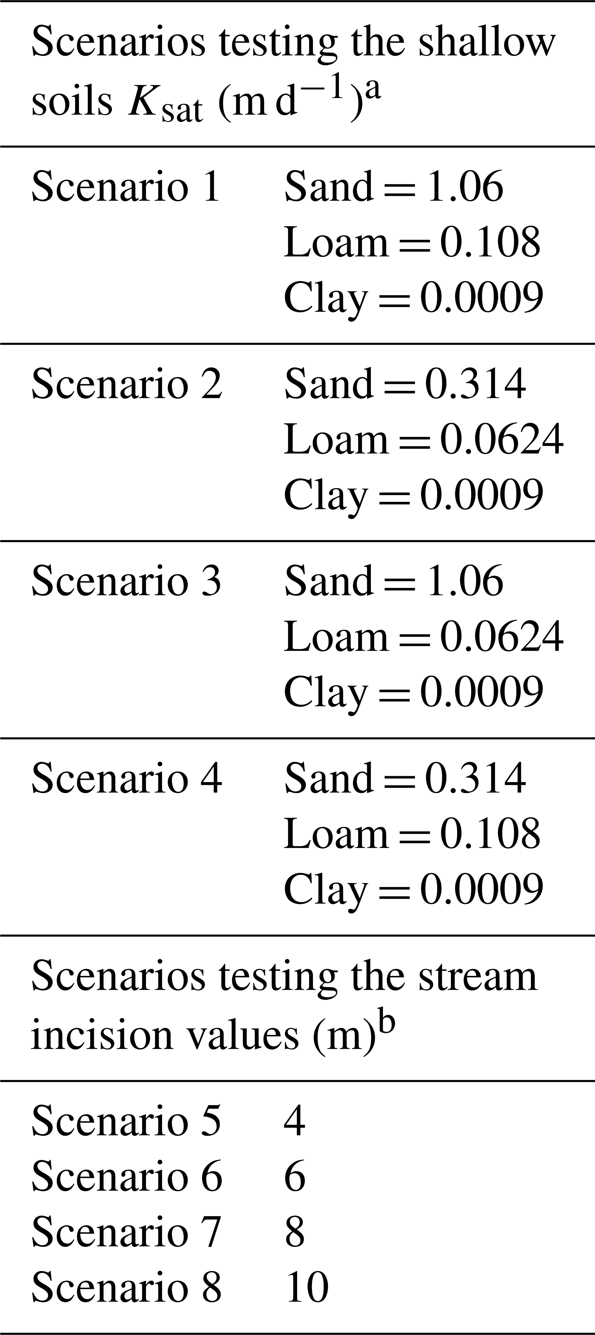
a For the corresponding unsaturated storage parameters, refer to Table 3. b Soil hydraulic properties for scenarios 5–8 are the same as those for scenario 4.
Model output for the surface domain (2D) was post-processed to identify and quantify the activation of areas (flow onset) and the flow generation mechanisms. The output files were processed in Python to determine the HMC fraction (flow generation mechanism) that contributed most of the flow (dominant fraction) at every single node and for each output time. Results of the dominant fraction were then included as a new variable to the overland output file. A water depth threshold equal to the rill storage height (0.01 m) was used to determine when an area was considered active (i.e. values of 0.01 m or less were considered as rill storage and not flow). Output for the porous media (3D) was used to support the HMC dominant fractions findings.
The computational demands of modelling a large and variably saturated domain subject to sudden state changes from dry to wet conditions led to extremely slow model convergence. From the set of scenarios testing different values for incising the stream (Table 4), only scenario 8 (incision = 10 m) finished within 2 months of run-time. Scenarios 5–7 showed less than 10 % of progress after 20 d of computation time. Nevertheless, the comparable results between scenario 8 and 4, which shared the same soil hydraulic properties but had the two ends of the spectrum with respect to the river incision (the most vs. none) suggest that results from scenarios 5–7 would have likely shown similar results. Therefore, from here on we will only focus on the results from scenarios 1–4 (different soil hydraulic properties) and 8 (river incised).
3.1 Active areas and dominant flow generation processes determined with HMC
The development of active areas (initiation of flow) in terms of the timing and extent was similar among scenarios 1–4, while for scenario 8 (scenario with the incised stream nodes) the aerial extent was consistently smaller (Fig. 5). Across all scenarios, flow was generated first on areas from the steep hills, and these areas expanded and contracted throughout the simulation. Fragmented active areas developed along the stream network for scenario 8, while for scenarios 1–4 the active areas along the stream developed as result of the flow from the hills connecting to stream network and expanding from there. Although the overall active areas along the river were larger for scenarios 1–4, a larger length of the stream network showed flow for scenario 8.
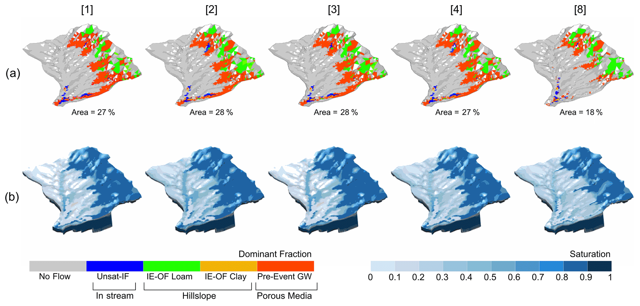
Figure 5Snapshots of time step 960 during a rainfall event showing (a) the spatial extent of active areas by their dominant HMC component (flow generation mechanism) for each scenario (1–4 and 8) and (b) the porous media saturation. The spatial extent of active areas as a percentage of the catchment area is shown below the snapshots. Colours for the HMC components show both the dominant process and the origin of the water contributing to the flow in each cell. For example, all red areas are from pre-event GW, some of which can contribute to active areas in both the stream and in the stream banks.
The development of active areas across scenarios matched the areas where the shallow soil profile reached saturation. The dominant flow generation mechanism on most of the steep hills shifted from IE-OF from the loam soil in the hill slopes during precipitation events to pre-event GW afterwards. A few small areas on the steep hills also showed unsaturated IF as the dominant mechanism. In the area near the outlet, the flow generation mechanisms during precipitation events included IE-OF from the clay hillslopes, in-stream unsaturated IF, and pre-event GW. After precipitation events, pre-event GW was prevalent on the areas near the outlet. The flow simulated in the few areas along the stream network close to the sandy areas from the mild hills simulated flow mostly through unsaturated IF.
3.2 Water balance comparisons
Among the scenarios with different sets of hydraulic properties (scenarios 1 through 4), the water balance breakdown was virtually identical for scenarios 2 and 3 (< 0.1 %) and 1 and 4 (∼ 0.1 %), and only small differences (as a percentage of the overall water balance) were observed between scenarios 2 and 3 and 1 and 4 (∼ 0.1 %–4 %; Fig. 6; also see the Supplement for a full breakdown of the water balance results). The results showed a higher porous media (PM) and overland flow (OLF) flux component and a smaller fluid transfer (FT) flux component for scenarios 2 and 3 than for scenarios 1 and 4. Since the change in storage is the sum of the OLF and PM components, scenarios 2 and 3 also showed a larger change in storage than scenarios 1 and 4. The largest differences in the water balance were simulated between scenarios 1–4 (no incised stream) and scenario 8 (incised stream). Scenario 8 had the largest OLF flux and change in storage and the smaller ET flux.
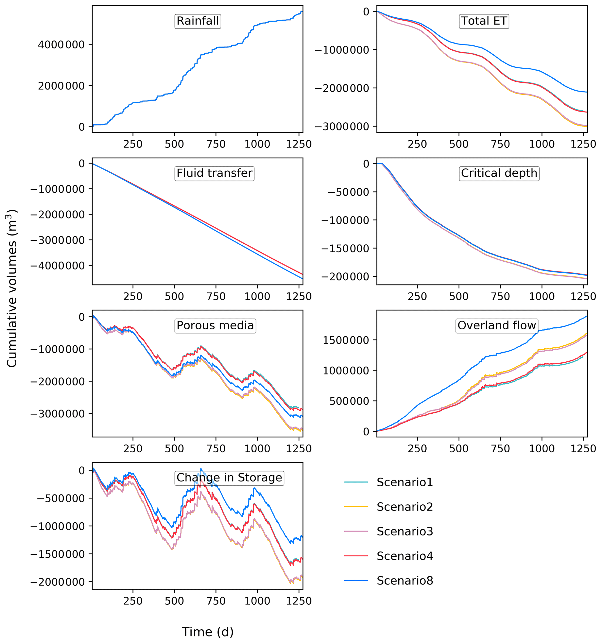
Figure 6Cumulative values of the water balance components simulated with HydroGeoSphere for scenarios 1–4 and 8.
The goals of this study were to provide insight into streamflow generation processes at the catchment scale for an intermittent Mediterranean climate catchment to better understand the importance of controlling characteristics identified during previous modelling efforts in non-perennial stream catchments (Table 1). This includes soil heterogeneity, as studies in both perennial and non-perennial catchments have shown that vertical soil heterogeneity can result in the development of perched saturated zones that contribute to flow generation (Hathaway et al., 2002; Maxwell and Kollet, 2008). Other studies indicated that horizontal heterogeneity contributed to the spatiotemporal variability in flow generation under different mechanisms which resulted in longer flow durations overall due to delays in runoff occurring from areas with high infiltration capacities (Ebel et al., 2016; Luce and Cundy, 1994; Smith and Hebbert, 1979).
In this study, we developed a conceptual framework of the hydrological processes identified in three distinct subregions of the Pedler Creek catchment. The steep hills are characterised by permeable shallow loam soils, steep slopes, and deep GW heads, which would result in sat-IF and SE-OF. The undulating hills are characterised by high permeable deep sandy soils, mild slopes, and deep GW heads, which would result in unsat-IF. The flat valley consisted of a mix of the previous soils, with the addition of a clay area, all located in low-gradient terrain and presenting the areas of shallow GW heads which would result in a mix of flow generation processes. We hypothesised that these distinct topographical conditions and soil types have a definite influence on streamflow generation mechanisms. However, although each catchment has its own set of conditions, most Mediterranean climate catchments would have similar topography to what was modelled here, with hills graduating to a coastal plain. Moreover, because the modelled catchment included a range of soil types, we were able to explore the variation in streamflow generation processes across several soil types. Moreover, it is likely that many other seasonally flowing catchments would have similar variation in soil, as the periodic and often flashy nature of streamflows carries fine material from the steeper headwaters and deposits it on the plains (Jaeger et al., 2017).
Model results overall supported our conceptual understanding that distinctive topographic and soil characteristics explain flow generating processes in Pedler Creek. Results from the active areas showed distinct mechanisms developing in the three major areas (Fig. 5), supporting the idea that there is a spatial and temporal variation in flow generation processes in Pedler Creek. In the model, flow developed first in the steep hills areas (fast flow), and the dominant mechanism was SE-OF, with a few areas showing unsat-IF as hypothesised in our conceptual model (Figs. 3b and 5). An unexpected development was the contribution of pre-event GW during flow recessions. In this area, the pre-event GW was likely to be pre-event soil water since an evaluation of the model showed that the groundwater level did not rise to intersect land surface in this area. The flows generated in the valley near the outlet were similarly simulated via the conceptualised mechanisms (Figs. 3d and 5). We saw small areas with flow originating from IE-OF from the clay areas and a combination of unsat-IF and pre-event GW for the rest of the active areas in this region. The GW did rise above the surface elevation in this area, supporting the GW contribution to flow in this area. Finally, in the few small areas close to the sandy undulating hills region, flow was simulated through the unsat-IF mechanism, as predicted in our conceptual framework (Figs. 3c and 5). These results support the findings by Gutierrez-Jurado et al. (2019), who suggested that soil properties largely dictate the dominant flow generation mechanisms and that unsaturated storage dynamics control the thresholds and pathways of flow. For real catchments such as Pedler Creek, soil properties and topography evolve in tandem, and it is impossible to fully disentangle their relative influence on streamflow generation. Such undulating and variable topography is not captured by theoretical models. The development and extent of active areas and the dominant flow generation mechanisms estimated by the HMC method and the water balance results were almost identical for scenarios 1–4, indicating that knowledge of the exact hydraulic conductivity value of a given soil type is less importance than capturing the general vertical and longitudinal soil heterogeneity across the catchment. The small differences simulated between scenarios 2 and 3 and 1 and 4 show that the models were more sensitive to variations in the hydraulic properties of the loam soil, as the scenarios with identical responses (2 and 3 and 1 and 4) shared the same loam but different sand hydraulic properties. The loam's smaller hydraulic conductivity for scenarios 2 and 3 (0.0624 m3 d−1) limited infiltration, which translated to more OLF. At the same time, the higher water holding capacity in the loam areas might have resulted in slower subsurface flows to either exfiltrate to the surface or to contribute to the fluid transfer (FT) through the subsurface boundary. In contrast, both tested values for the sand resulted in a low water holding capacity that allowed the incoming precipitation to drain past the root zone and move in the subsurface contributing to the FT. This is supported by the higher FT values shown for scenarios 1 and 4 (Fig. 6).
The greatest differences for both the water balance and HMC results among the tested scenarios were caused by differences in stream definition between scenarios 1–4 (no incised stream) and scenario 8 (incised stream). The effects of the incised stream in scenario 8 resulted in a larger OLF flux, a smaller ET flux, and in an overall smaller extent of active areas (Fig. 5 and Supplement). The roles of a good channel representation in ISSHMs is extensively discussed by Käser et al. (2014). While their discussion of channel representation revolves on the ability of ISSHMs to quantify GW–stream interactions (which was not a major component for this model), the hydrological principles are relevant and transferable to explain the importance of channel representation to capture streamflow generation processes. Without a defined channel, the connection to the Pedler Creek floodplain was lost, and the shallow sheet flow and most of the precipitation infiltrated and stayed within the porous media. The importance of the connection of the floodplain to the channel is also discussed by Käser et al. (2014), as they argued that not only is the channel topography important but also its connection to the floodplain, given that riverbank geometry is key for bank storage and overbank flooding. Although overbank flooding is not considered important for this study (flows in Pedler only rarely will experience overbank flooding), the stream–floodplain connectivity and bank storage were key aspects under our model conceptualisation. That is, the predicted dominant mechanisms relied upon the saturation to build up along the riverine zone in the loamy areas, which would lead to saturation excess overland flow. We expected a perched groundwater to develop on the sandy hillslopes which would, after intersecting the stream, contribute with interflow into the stream. While we observed as these processes developed, they only occurred briefly as very shallow runoff.
Another important consideration for the channel representation in streamflow generation studies for non-perennial streams is the relationship between flow and the wetted area. The larger the channel (both vertically and horizontally), the larger the area of exchange to the unsaturated zones during a flow event (Doble et al., 2012), which would be exacerbated under low flows (Käser et al., 2014). This is particularly significant when evaluating streamflow generation for non-perennial streams where high streambed infiltration and transmission losses are common (Gutierrez-Jurado et al., 2019; Levick et al., 2008; Shanafield and Cook, 2014; Snelder et al., 2013) and often prevent flows from even reaching the catchment outlet (Keppel and Renard, 1962; Aldridge, 1970). In this study, we observed that, without a defined stream to channel the water, the little overland flow that was simulated in scenarios 1–4 (no incised stream) spread over a larger area than in scenario 8 where the stream was incised (Fig. 5). The same was true for the patterns of increased saturation of the porous media across the catchment (Fig. 6). Results from the water balance reflected the effects of having both flows and porous media saturation spread over larger areas by exacerbating ET and decreasing the overall amount of overland flow for scenarios 1–4 (see the Supplement). This is consistent with the remarks by Käser et al. (2014) regarding the likely impacts to the water flow budget by the spatiotemporal aspects linked to channel representation due to spatial exchange patterns.
Finally, this study highlighted both the need for further studies examining streamflow generation processes in additional non-perennial catchments. For instance, our results underlined the importance of channel representation, and future studies should investigate the effects of channel morphology in streamflow generation in non-perennial catchments. Moreover, while for Pedler Creek the GW–stream interactions were conceptualised to occur only near the catchment outlet (and likely only during certain wet years), flow intermittence in many rivers can be attributed to a water table fluctuation relative to the stream channel elevation (Snelder et al., 2013). Future work on flow intermittence as a result of GW–stream interactions would be valuable. Similarly, the inherent challenges associated with capturing unsaturated zone dynamics at the catchment scale were underpinned in this study. Indeed, modelling this non-perennial river system confirmed the inherent difficulties of using ISSHMs in medium-sized non-perennial river catchments and reiterated why so few studies have been done on this topic. Extensive work was needed to set up this model, and the large computational time to run the simulations was a major constraint to both establishing initial conditions and exploring scenarios. For example, when draining the model, simulations running for over 10 d only progressed to day 100 of the simulation. Relaxing the mesh allowed us to develop reasonable initial conditions after testing over 37 scenarios. For the scenarios running for the full 4-year simulation, simulation convergence consistently slowed down when the simulation encountered a precipitation input, particularly during prolonged precipitation events (i.e. consecutive precipitation inputs), which is expected given the highly nonlinear equations for unsaturated flow in the unsaturated surface domain. Despite the conceptual advantages of using a fully physically based model to explicitly capture all surface and groundwater processes, future studies may try to identify a suitable simplified surrogate model to speed up simulations and focus on specific areas where particular streamflow generation processes are thought to be dominant.
There are hundreds of similar non-perennial river systems in the semi-arid coastal Mediterranean climate regions of South Australia, Western Australia, California, South Africa, and around the Mediterranean itself (Davies et al., 1993; Tzoraki and Nikolaidis 2007; Skoulikidis et al., 2017). This study provides an initial step towards understanding non-perennial streamflow generation processes at the catchment scale and provides a template for using ISSHMs for process understanding in these stream systems. The development of a conceptual model of the most important factors impacting flow generation processes within Pedler catchment presented a hypothesis that combined our understanding of field data with lessons learnt from previous studies. This conceptualisation informed the model setup and captured the dynamics of streamflow generation in this non-perennial stream system. Difficulties in setting up and running the model reaffirmed the numerical difficulties experienced in large-scale unsaturated models, such as accurately reproducing the topography and observed initial conditions, was a challenge. Model runtimes prohibited extensive exploration of multiple scenarios. In particular, the importance of preserving channel representation to model streamflow generation on non-perennial systems became apparent in the scenarios. Yet, overall, the model results confirmed our conceptual understanding that soil type, unsaturated storage dynamics, and topography are major controls for streamflow generation processes in non-perennial streams. The similarity in the results from scenarios comparing soil hydraulic properties across the literature range for each soil type showed that exact knowledge of these values for a given soil type is not critical for identifying streamflow generation processes if the conceptual model is accurate and the vertical and longitudinal soil heterogeneity is captured. Given that soil properties are often highly heterogeneous within a catchment and rarely well known, this result is will be important for future modelling studies.
The data for this model were sourced through publicly available resources, as cited in Sect. 2. Commercially available AlgoMesh (HydroAlgorithmics) software and HydroGeoSphere (Aquanty) software were used to prepare and run the model simulations. Model files and processing routines are available at https://doi.org/10.5281/zenodo.4722110 (Partington, 2021).
The supplement related to this article is available online at: https://doi.org/10.5194/hess-25-4299-2021-supplement.
KYGJ, MS, and DP conceived the project design. KYGJ developed the conceptual model. KYGJ developed the numerical model, with assistance from DP. KYGJ and MS prepared the paper, with contributions from all co-authors.
The authors declare that they have no conflict of interest.
Publisher’s note: Copernicus Publications remains neutral with regard to jurisdictional claims in published maps and institutional affiliations.
This article is part of the special issue “Data acquisition and modelling of hydrological, hydrogeological and ecohydrological processes in arid and semi-arid regions”. It is not associated with a conference.
The authors thank the editor and the two anonymous reviewers for their valuable comments which improved this paper.
This research has been supported by the Australian Research Council (grant no. DE150100302).
This paper was edited by Insa Neuweiler and reviewed by two anonymous referees.
Aldam, R. G.: Willunga Basin hydrogeological investigations 1986/88, South Australia Department of Mines and Energy, Report Book, 89/22, Government of South Australia, Adelaide, Australia, 1989.
Aldam, R. G.: Willunga Basin Groundwater Investigation Summary Report. Groundwater and Engineering, Department of Mines and Energy, Government of South Australia, Report Book, 90/71, Government of South Australia, Adelaide, Australia, 1990.
Aldridge, B. N.: Floods of November 1965 to January 1966 in the Gila River basin, Arizona and New Mexico, and adjacent basins in Arizona, US Geological Survey Water-Supply Paper 1850-C, 176 pp., https://doi.org/10.3133/wsp1850C, 1970.
Ambroise, B.: Variable “active” versus “contributing” areas or periods: A necessary distinction, Hydrol. Process., 18, 1149–1155, https://doi.org/10.1002/hyp.5536, 2004.
Anders, L.: Surface – Water and Groundwater Interactions Along Pedler Creek, MSc Thesis, Flinders University, Adelaide SA, Australia, 2012.
Aquanty: HydroGeoSPhere user manual, Release 1.0, Aquanty Inc, Waterloo, Ontario, Canada, 2016.
Banks, E. W., Brunner, P., and Simmons, C. T.: Vegetation controls on variably saturated processes between surface water and groundwater and their impact on the state of connection, Water Resour. Res., 47, 1–14, https://doi.org/10.1029/2011WR010544, 2011.
Batlle-Aguilar, J. and Cook, P. G.: Transient infiltration from ephemeral streams: A field experiment at the reach scale, Water Resour. Res., 48, W11518, https://doi.org/10.1029/2012WR012009, 2012.
Beven, K.: Runoff generation in semi-arid areas, in: Dryland Rivers: Hydrology and geomorphology, edited by: Bull, L. J. and Kirkby, M. J., John Wiley & Sons, Ltd., Chichester, UK, 2002.
Blasch, K. W., Ferré, T. P. A., Hoffmann, J. P., and Fleming, J. B.: Relative contributions of transient and steady state infiltration during ephemeral streamflow, Water Resour. Res., 42, W08405, https://doi.org/10.1029/2005WR004049, 2006.
Brown, K. G.: Groundwater contributions to streamflow along Willunga Fault, McLaren Vale, South Australia, Report DWLBC 2004/21, Department of Water, Land and Biodiversity Conservation, Adelaide SA, Australia, 2004.
Brunner, P. and Simmons, C. T.: HydroGeoSphere: A fully integrated, physically based hydrological model, Ground Water, 50, 170–176, https://doi.org/10.1111/j.1745-6584.2011.00882.x, 2012.
Campana, M. E. and Simpson, E. S.: Groundwater residence times and recharge rates using a discrete-state compartment model and 14C data, J. Hydrol., 72, 171–185, https://doi.org/10.1016/0022-1694(84)90190-2, 1984.
Carr, A. E., Loague, K., and VanderKwaak, J. E.: Hydrologic-response simulations for the North Fork of Caspar Creek: Second-growth, clear-cut, new-growth, and cumulative watershed effect scenarios, Hydrol. Process., 28, 1476–1494, https://doi.org/10.1002/hyp.9697, 2014.
Carsel, R. F. and Parrish, R. S.: Developing Joint Probability-Distributions of Soil-Water Retention Characteristics, Water Resour. Res., 24, 755–769, 1988.
Chow, V. T.: Open channel hydraulics, McGraw-Hill, New York, USA, p. 680, 1959.
Costigan, K. H., Kennard, M. J., Leigh, C., Sauquet, E., Datry, T., and Boulton, A. J.: Flow regimes in intermittent river and ephemeral streams, in: Intermittent Rivers: Ecology and Management edited by: Datry, T., Bonada, N., and Boulton, A., Academic press, p. 300, https://doi.org/10.1016/C2015-0-00459-2, 2017.
Cudennec, C., Leduc, C., and Koutsoyiannis, D.: Dryland hydrology in Mediterranean regions – A review, Hydrol. Sci. J., 52, 1077–1087, https://doi.org/10.1623/hysj.52.6.1077, 2007.
Davies, B. R., O’keeffe, J. H., and Snaddon, C. D.: A synthesis of the ecological functioning, conservation and management of South African river ecosystems, WRC Report No. TT 62/63, Water Research Commission, Pretoria, South Africa, 1993.
DEW: Soils (soil type), Department for Environment and Water, available at: https://data.sa.gov.au/data/dataset/soil-type (last access: 10 June 2018), 2016.
DEWNR: Soil and Land Program: Soil Characterisation Sites, available at: https://data.sa.gov.au/data/dataset/soil-characterisation-sites (last access: 10 June 2018), 2016.
Di Giammarco, P., Todini, E., and Lamberti, P.: A conservative finite elements approach to overland flow: The control volume finite element formulation, J. Hydrol., 175, 267–291, https://doi.org/10.1016/S0022-1694(96)80014-X, 1996.
Doble, R., Brunner, P., McCallum, J., and Cook, P. G.: An analysis of river bank slope and unsaturated flow effects on bank storage, Groundwater, 50, 77-86, https://doi.org/10.1111/j.1745-6584.2011.00821.x, 2012.
Ebel, B. A., Rengers, F. K., and Tucker, G. E.: Observed and simulated hydrologic response for a first-order catchment during extreme rainfall 3 years after wildfire disturbance, Water Resour. Res., 52, 9367–9389, https://doi.org/10.1002/2016WR019110, 2016.
Fekete, B. M. and Vörösmarty, C. J.: The current status of global river discharge monitoring and potential new technologies complementing traditional discharge measurements, in: Predictions in Ungauged Basins: PUB Kick-off, Proceedings of the PUB Kick-off Meeting, 20–22 November 2002, Brasilia, Brazil, IAHS Publ., 309, 129–136, IAHS, Wallingford, UK, 2007.
Geeroms, J.: 3D modeling to evaluate infiltration furrows for rainwater harvesting in the semiarid zone of Chile, Thesis, Department of Soil Management, Ghent University, Ghent, Belgium, 110 pp., 2009.
Gutierrez-Jurado, K. Y., Partington, D., Batelaan, O., Cook, P., and Shanafield, M.: What triggers streamflow for Intermittent Rivers and Ephemeral Streams in Low-Gradient Catchments in Mediterranean Climates, Water Resour. Res., 55, 9926–9946, https://doi.org/10.1029/2019WR025041, 2019.
Hall, J. A. S., Maschmedt, D. J., and Billing, N. B.: The soils of Southern South Australia. The South Australian Land and Soil Book Series, vol. 1, Geological Survey of South Australia, Bulletin 56, vol. 1, Government of South Australia, Adelaide, Australia, 2009.
Harrington, G. A.: Recharge mechanisms to Quaternary sand aquifers in the Willunga Basin, South Australia, Department of Water, Land and Biodiversity Conservation, Adelaide, SA, Australia, 2002.
Hathaway, D. L., Ha, T. S., and Hobson, A.: Transient Riparian Aquifer and Stream Exchanges along the San Joaquin Stream, in: Proceedings of the Ground Water/Surface Water Interactions, AWRA 2002 Summer Specialty Conference, 1–3 July 2002, Colorado, USA, 169–174, 2002.
Heppner, C. S., Loague, K., and VanderKwaak, J. E.: Long-term InHM simulations of hydrologic response and sediment transport for the R-5 catchment, Earth Surf. Proc. Land., 32, 1273–1292, https://doi.org/10.1002/esp.1474, 2007.
Hingston, F. J., Galbraith, J. H., and Dimmock, G. M.: Application of the process-based model BIOMASS to Eucalyptus globules subsp. Globules plantations on ex-farmland in south Western Australia: I. Water use by trees and assessing risk of losses due to drought, Forest Ecol. Manage., 106, 141–156, 1997.
Irvine, M. L.: Using tracers to determine groundwater fluxes in a coastal aquitard-aquifer system, PhD Thesis, Flinders University, Adelaide, SA, Australia, 2016.
Jaeger, K., Sutfin, N. A., Tooth, S., Michaelides, K., and Singer, M.: Geomorphology and Sediment Regimes of Intermittent Rivers and Ephemeral Streams, chap. 2, in: Intermittent Rivers and Ephemeral Streams, Academic Press, 21–49, https://doi.org/10.1016/B978-0-12-803835-2.00002-4, 2017.
Käser, D., Graf, T., Cochand, F., Mclaren, R., Therrien, R., and Brunner, P.: Channel Representation in Physically Based Models Coupling Groundwater and Surface Water: Pitfalls and How to Avoid Them, Groundwater, 52, 827–836, https://doi.org/10.1111/gwat.12143, 2014.
Keppel, R. V. and Renard, K. G.: Transmission losses in ephemeral stream beds, J. Hydraul. Div., 88, 59-68, 1962.
Knowles, I., Teubner, M., Yan, A., Rasser, P., and Lee, J. W.: Inverse groundwater modelling in the Willunga Basin, South Australia, Hydrogeol. J., 15, 1107–1118, https://doi.org/10.1007/s10040-007-0189-6, 2007.
Kollet, S., Sulis, M., Maxwell, R. M., Paniconi, C., Putti, M., Bertoldi, G., Coon, E. T., Cordano, E., Endrizzi, S., Kikinzon, E., Mouche, E., Mügler, C., Park, Y. J., Refsgaard, J. C., Stisen, S., and Sudicky, E.: The integrated hydrologic model intercomparison project, IH-MIP2: A second set of benchmark results to diagnose integrated hydrology and feedbacks, Water Resour. Res., 53, 867–890, https://doi.org/10.1002/2016WR019191, 2017.
Kristensen, K. J. and Jensen, S. E.: A model for estimating actual evapotranspiration from potential evapotranspiration, Hydrol. Res., 6, 170–188, https://doi.org/10.2166/nh.1975.0012, 1975.
Levick, L. R., Goodrich, D. C., Hernandez, M., Fonseca, J., Semmens, D. J., Stromberg, J. C., Tluczek, M., Leidy, R. A., Scianni, M., Guertin, D. P., and Kepner, W. G.: The ecological and hydrological significance of ephemeral and intermittent streams in the arid and semi-arid American Southwest, U.S. Environmental Protection Agency, Office of Research and USDA/ARS Southwest Watershed Research Center, EPA/600/R-08/134, ARS/233046, Washington, DC, USA, 2008.
Liggett, J. E., Werner, A. D., Smerdon, B. D., Partington, D., and Simmons, C. T.: Fully integrated modeling of surface-subsurface solute transport and the effect of dispersion in tracer hydrograph separation, Water Resour. Res., 50, 7750–7765, https://doi.org/10.1002/2013WR015040, 2014.
Luce, C. H. and Cundy, T. W.: Parameter identification for a runoff model for forest roads, Water Resour. Res., 30, 1057–1069, https://doi.org/10.1029/93WR03348, 1994.
Martin, R. R.: Willunga Basin – Status of Groundwater Resources 1998, Department of Primary Industries and Resources, Report Book 98/28, Adelaide, South Australia, Australia, 1998.
Martin, R. R.: Hydrogeology and Numerical Groundwater Flow Model for the McLaren Vale Prescribed Wells Area Summary Report, REM, Adelaide and Mount Lofty Ranges Natural Resource Management Board, South Australia, Adelaide, Australia, 2006.
Maxwell, R. M. and Kollet, S. J.: Quantifying the effects of three-dimensional subsurface heterogeneity on Hortonian runoff processes using a coupled numerical, stochastic approach, Adv. Water Resour., 31, 807–817, https://doi.org/10.1016/j.advwatres.2008.01.020, 2008.
Measurement Engineering Australia (MEA): Weather station data, available at: https://weathermclarenvale.info/observations, last access: 28 March 2019.
Merheb, M., Moussa, R., Abdallah, C., Colin, F., Perrin, C., and Baghdadi, N.: Hydrological response characteristics of Mediterranean catchments at different time scales: a meta-analysis, Hydrol. Sci. J., 61, 2520–2539, https://doi.org/10.1080/02626667.2016.1140174, 2016.
Meyerhoff, S. B. and Maxwell, R. M.: Quantifying the effects of subsurface heterogeneity on hillslope runoff using a stochastic approach, Hydrogeol. J., 19, 1515–1530, https://doi.org/10.1007/s10040-011-0753-y, 2011.
Mihevc, T., Pohll, G., Niswonger, R., and Stevick, E.: Truckee Canal seepage analysis in the Frenley/Wadsworth area, Rep. 41176, 45 pp., Desert Res. Inst., Univ. of Nev., Las Vegas, Nev., USA, 2002.
Milly, P. C. D., Dunne, K. A., and Vecchia, A. V.: Global pattern of trends in streamflow and water availability in a changing climate, Nature, 438, 347–350, https://doi.org/10.1038/nature04312, 2005.
Mirus, B. B. and Loague, K.: How runoff begins (and ends): Characterizing hydrologic response at the catchment scale, Water Resour. Res., 49, 2987–3006, https://doi.org/10.1002/wrcr.20218, 2013.
Mirus, B. B., Loague, K., VanderKwaak, J. E., Kampf, S. K., and Burges, S. J.: A hypothetical reality of Tarrawarra-like hydrologic response, Hydrol. Process., 23, 1093–1103, https://doi.org/10.1002/hyp.7241 A, 2009.
Mirus, B. B., Loague, K., Cristea, N. C., Burges, S. J., and Kampf, S. K.: A synthetic hydrologic-response dataset, Hydrol. Process., 25, 3688–3692, https://doi.org/10.1002/hyp.8185, 2011a.
Panday, S. and Huyakorn, P. S.: A fully coupled physically-based spatially-distributed model for evaluating surface/subsurface flow, Adv. Water Resour., 27, 361–382, https://doi.org/10.1016/j.advwatres.2004.02.016, 2004.
Partington, D.: daniel-partington/Pedler_creek_streamflow_generation: Model_input_files_for_Pedler_Creek (Version 1.0), Zenodo [code], https://doi.org/10.5281/zenodo.4722110, 2021.
Partington, D., Brunner, P., Simmons, C. T., Therrien, R., Werner, A. D., Dandy, G. C., and Maier, H. R.: A hydraulic mixing-cell method to quantify the groundwater component of stream flow within spatially distributed fully integrated surface water-groundwater flow models, Environ. Model. Softw., 26, 886–898, https://doi.org/10.1016/j.envsoft.2011.02.007, 2011.
Partington, D., Brunner, P., Frei, S., Simmons, C. T., Werner, A. D., Therrien, R., Maier, H. R., Dandy, G. C., and Fleckenstein, J. H.: Interpreting streamflow generation mechanisms from integrated surface-subsurface flow models of a riparian wetland and catchment, Water Resour. Res., 49, 5501–5519, https://doi.org/10.1002/wrcr.20405, 2013.
Pierini, N. A., Vivoni, E. R., Robles-Morua, A., Scott, R. L., and Nearing, M. A.: Using observations and a distributed hydrologic model to explore runoff thresholds linked with mesquite encroachment in the Sonoran Desert, Water Resour. Res., 50, 8191–8215, https://doi.org/10.1002/2014WR015781, 2014.
Poff, N. L. R., Bledsoe, B. P., and Cuhaciyan, C. O.: Hydrologic variation with land use across the contiguous United States: Geomorphic and ecological consequences for stream ecosystems, Geomorphology, 79, 264–285, https://doi.org/10.1016/j.geomorph.2006.06.032, 2006.
Schaap, M. G., Leij, F. J., and van Genuchten, M. T.: ROSETTA: a computer program for estimating soil hydraulic parameters with hierarchical pedotransfer functions, J. Hydrol., 251, 163–176, https://doi.org/10.1016/S0022-1694(01)00466-8, 2002.
Sereda, A. and Martin, R. R.: Willunga groundwater basin observation well network monitoring and trends in aquifers, Resource Assessment Division, Report DWR 2001/015, Dept. for Water Resources, Adelaide, Australia, 2000.
Shanafield, M. and Cook, P. G.: Transmission losses, infiltration and groundwater recharge through ephemeral and intermittent streambeds: A review of applied methods, J. Hydrol., 511, 518–529, https://doi.org/10.1016/j.jhydrol.2014.01.068, 2014.
Shanafield, M., Bourke, S., Zimmer, M., and Costigan, K.: Overview of the hydrology of non-perennial rivers and streams, Wiley Interdiscip. Rev. Water., 8, e1504, https://doi.org/10.1002/wat2.15042021, 2021.
SILO: Australian Climate Data, Station 232729 climate records, available at: https://www.longpaddock.qld.gov.au/silo/, last access: 28 March 2019.
Skoulikidis, N. T., Sabater, S., Datry, T., Morais, M. M., Buffagni, A., Dörflinger, G., Zogaris, S., Sánchez-Montoya, M. M., Bonada, N., Kalogianni, E., Rosado, J., Vardakas, L., De Girolamo A. M., and Tockner, K.: Non-perennial Mediterranean Rivers in Europe: Status, pressures, and challenges for research and management, Sci. Total Environ., 577, 1–18, https://doi.org/10.1016/j.scitotenv.2016.10.147, 2017.
Smith, R. E. and Hebbert, R. H. B.: A Monte Carlo analysis of the hydrologic effects of spatial variability of infiltration, Water Resour. Res., 15, 419–429, https://doi.org/10.1029/WR015i002p00419, 1979.
Snelder, T. H., Datry, T., Lamouroux, N., Larned, S. T., Sauquet, E., Pella, H., and Catalogne, C.: Regionalization of patterns of flow intermittence from gauging station records, Hydrol. Earth Syst. Sci., 17, 2685–2699, https://doi.org/10.5194/hess-17-2685-2013, 2013.
Therrien, R., McLaren, R. G., Sudicky, E. A., and Panday, S. M.: HydroGeoSphere: A three-dimensional numerical model describing fully-integrated subsurface and surface flow and solute transport, Groundwater Simulations Group, Waterloo, Ont., Canada, 2010.
Tzoraki, O. and Nikolaidis, N. P: A generalized framework for modeling the hydrologic and biogeochemical response of a Mediterranean temporary river basin, J. Hydrol., 346, 112–121, https://doi.org/10.1016/j.jhydrol.2007.08.025, 2007.
VanderKwaak, J. E. and Loague, K.: Hydrologic-response simulations for the R-5 catchment with a comprehensive physics-based model, Water Resour. Res., 37, 999–1013, https://doi.org/10.1029/2000WR900272, 2001.
Vivoni, E. R., Entekhabi, D., Bras, R. L., and Ivanov, V. Y.: Controls on runoff generation and scale-dependence in a distributed hydrologic model, Hydrol. Earth Syst. Sci., 11, 1683–1701, https://doi.org/10.5194/hess-11-1683-2007, 2007.
Water Data Services: Pedler Creek @ Stump Hill Road – A5030543, AMLR, available at: https://greenadelaide.waterdata.com.au/StationDetails.aspx?sno=A5030543, last access: 10 March 2019.
Weill, S., Altissimo, M., Cassiani, G., Deiana, R., Marani, M., and Putti, M.: Saturated area dynamics and streamflow generation from coupled surface–subsurface simulations and field observations, Adv. Water Resour., 59, 196–208, https://doi.org/10.1016/j.advwatres.2013.06.007, 2013.
Wigmosta, M. S., Vail, L. W., and Lettenmaier, D. P.: A distributed hydrology-vegetation model for complex terrain, Water Resour. Res., 30, 1665–1679, https://doi.org/10.1029/94WR00436, 1994.
Ye, W., Bates, B. C., Viney, N. R., Sivapalan, M., and Jakeman, A. J.: Performance of conceptual rainfall-runoff models in low-yielding ephemeral catchments, Water Resour. Res., 33, 153–166, https://doi.org/10.1029/96WR02840, 1997.