the Creative Commons Attribution 4.0 License.
the Creative Commons Attribution 4.0 License.
 | 03 Aug 2021
Mass balance and hydrological modeling of the Hardangerjøkulen ice cap in south-central Norway
Trude Eidhammer
Adam Booth
Sven Decker
Michael Barlage
David Gochis
Roy Rasmussen
Kjetil Melvold
Atle Nesje
Stefan Sobolowski
A detailed, physically based, one dimensional column snowpack model (Crocus) has been incorporated into the hydrological model, Weather Research and Forecasting (WRF)-Hydro, to allow for direct surface mass balance simulation of glaciers and subsequent modeling of meltwater discharge from glaciers. The new system (WRF-Hydro/Glacier) is only activated over a priori designated glacier areas. This glacier area is initialized with observed glacier thickness and assumed to be pure ice (with corresponding ice density). This allows for melting of the glacier to continue after all accumulated snow has melted. Furthermore, the simulation of surface albedo over the glacier is more realistic, as surface albedo is represented by snow, where there is accumulated snow, and glacier ice, when all accumulated snow is melted. To evaluate the WRF-Hydro/Glacier system over a glacier in southern Norway, WRF atmospheric model simulations were downscaled to 1 km grid spacing. This provided meteorological forcing data to the WRF-Hydro/Glacier system at 100 m grid spacing for surface and streamflow simulation. Evaluation of the WRF downscaling showed a good comparison with in situ meteorological observations for most of the simulation period. The WRF-Hydro/Glacier system reproduced the glacier surface winter/summer and net mass balance, snow depth, surface albedo and glacier runoff well compared to observations. The improved estimation of albedo has an appreciable impact on the discharge from the glacier during frequent precipitation periods. We have shown that the integrated snowpack system allows for improved glacier surface mass balance studies and hydrological studies.
- Article
(14743 KB) - Full-text XML
- BibTeX
- EndNote


Glaciers provide natural storage of water supply to rivers. In Norway, these rivers can then contribute water for domestic and industrial consumption, irrigation and hydropower (Sorg et al., 2012; Laghari, 2013; Kaser et al., 2010). Glaciers are among the first indicators of climate variability and change, and thus, glacier retreat and changes and associated streamflow effects can impact human water supplies, depending on the modifications to glacier melt timing and amount (Immerzeel et al., 2013; Bolch et al., 2012). It is imperative to understand how glaciers and associated hydrological processes respond to a changing climate to better inform communities that rely on glaciers for their livelihoods and well-being.
It is the surface mass balance on glaciers that impacts the subsequent glacier-fed streamflow. Mass balance changes in glaciers in Norway are largely controlled by accumulation season precipitation and ablation season temperature. This was determined by comparing measured glacier mass balance from stake measurements with meteorological station data (winter precipitation and summer temperature; e.g., Andreassen and Winsvold, 2012). However, elevation gradients and complex topography in many glaciated regions lead to large variations in temperature, precipitation and winds (and, thereby, transport and deposition of dry snow during the accumulation season) and net radiative exchange across the glacier (e.g., Ayala et al., 2015; Liston and Sturm, 1998). Therefore, the proper simulation of the non-homogenous, non-stationary evolution of a glacier requires atmospheric processes at a much finer resolution than typical global or regional climate models can provide (Aas et al., 2016).
Obtaining distributed meteorological forcing data of temperature, precipitation and wind is complicated by the spatial and temporal scarcity of observations, topographic complexity and by the coarseness of the atmospheric models used for downscaling. As a result, there are major gaps in our knowledge regarding the behavior of glaciers at local to regional scales and the processes that control their variability (Immerzeel et al., 2010; Bolch et al., 2012). Several studies have used dynamical downscaling of regional climate models of the order of 10–18 km (e.g., Machguth et al., 2009; Kotlarski et al., 2010a; van Pelt et al., 2012). However, they still do not resolve many subgrid processes, and the studies have, therefore, required statistical corrections to the downscaling as well. Recently, several studies applied much higher resolution (0.5–2.5 km) regional climate models to provide the heterogeneous forcing required over glaciers (e.g., Collier et al., 2013, 2015; Aas et al., 2016; Mölg and Kaser, 2011; Bonekamp et al., 2019; Vionnet et al., 2019). Indeed, Lundquist et al. (2019) argue that, in many instances in mountain terrain, high-resolution atmospheric models produce better estimates of annual precipitation than the information we can gain from observation networks. Physically based downscaling based on the linear model by Smith and Barstad (2004) has also been applied over complex terrain for glacier studies (e.g., Jarosch et al., 2012). Glacier mass balance parameterizations have been implemented in atmospheric models such as the regional scale model REMO (REgional MOdel; Kotlarski et al., 2010b) and a climate mass balance model with feedback to the atmosphere was implemented into Weather Research and Forecasting (WRF) by Collier et al. (2013).
The regional atmosphere-only models typically do not have detailed information about runoff routing processes, which are important components in the glacier hydrological cycle, although these models can provide input to detailed offline snowpack and hydrological models. Glacier melt contributes to discharge, especially during summer when the magnitude of the summer peak river flow often depends on the contribution of melt water from snow and ice to the total river flow. This contribution from glaciers to total flow plays a key role in the glacier-fed rivers in populated regions in Norway in which summer flows are crucial for irrigation, human consumption and energy production. In the studies here, we will use the detailed hydrological model – WRF-Hydro – modeling system (Gochis et al., 2015; Senatore et al., 2015; Arnault et al., 2018; Fersch et al., 2020; Rummler et al., 2019) for streamflow modeling. However, WRF-Hydro does not explicitly include glaciers within the modeling system, which results in a large uncertainty and underestimation of discharge during the melt season in glacial-fed areas like the Himalayas (Li et al., 2017), parts of the Andes, Scandinavia and North America. The Noah multi-parameterization (Noah-MP; Niu et al., 2011) land surface model (LSM) is often used in the existing WRF-Hydro system, which includes only a glacier–land surface category. When snow is accumulated, Noah-MP uses a three-layer snow model to represent the evolution of the snowpack. However, when the seasonally accumulated snow melts off in the summer, the underlying surface, for albedo purposes, is assumed to be old snow (snowpacked glacier), while not allowing for areas of bare ice and melting ice. Furthermore, the glacier is also represented in the soil layer with a 2 m layer of ice and/or water at the bottom of the column. This layer can melt and refreeze, but this layer does not provide runoff to WRF-Hydro.
By linking a surface mass balance glacier model to the WRF-Hydro system that interacts with the underlying land surface–hydrological components, the coupled interactions between the energy, water and mass balance budgets over glaciated river basins can be better depicted for projecting future impacts. For this purpose, we chose the Crocus snow model as our starting point to build the system WRF-Hydro/Glacier. Crocus is a one-dimensional, column energy and mass model of snow and ice cover that uses meteorological conditions as input data and was initially developed for operational avalanche forecasting and simulation of Alpine snow (Brun et al., 1989, 1992). It is a physically based model in which the snow depth can be divided into user-defined maximum levels and where the default maximum is 50 layers. A principal strength of the model is the detailed description of the metamorphism process for different types of snow, which allows for a more accurate calculation of snow surface albedo. The Crocus model was first used for glacier mass balance studies by Gerbaux et al. (2005) and recently used for glacier surface mass balance studies within the French SURFEX model by Réveillet et al. (2018), Revuelto et al. (2016) and Vionnet et al. (2019).
Norway is home to some of the best-observed glaciers in the world. Its National Water Resource and Energy Directorate (NVE) regularly monitors and assesses the mass balance and length changes of Norwegian glaciers (Andreassen et al., 2020). This paper will focus on the Hardangerjøkulen ice cap, located in south-central Norway. Hardangerjøkulen is the sixth-largest glacier on the mainland of Norway and is located at the main water divide between eastern and western Norway. The glacier covers an area of approximately 71 km2, and the highest point on the glacier is 1863 m a.s.l. (above sea level; Andreassen and Winsvold, 2012). Hardangerjøkulen is a plateau glacier and has several outlet glaciers, of which Blåisen (not shown) and Midtdalsbreen, facing east/northeast, and Rembesdalskåka in the west are the best known (Fig. 1). The ice cap has a volume of about 10.64 km3, and the mean ice thickness is about 150 m, with a maximum ice thickness of more than 380 m (Melvold et al., 2011).
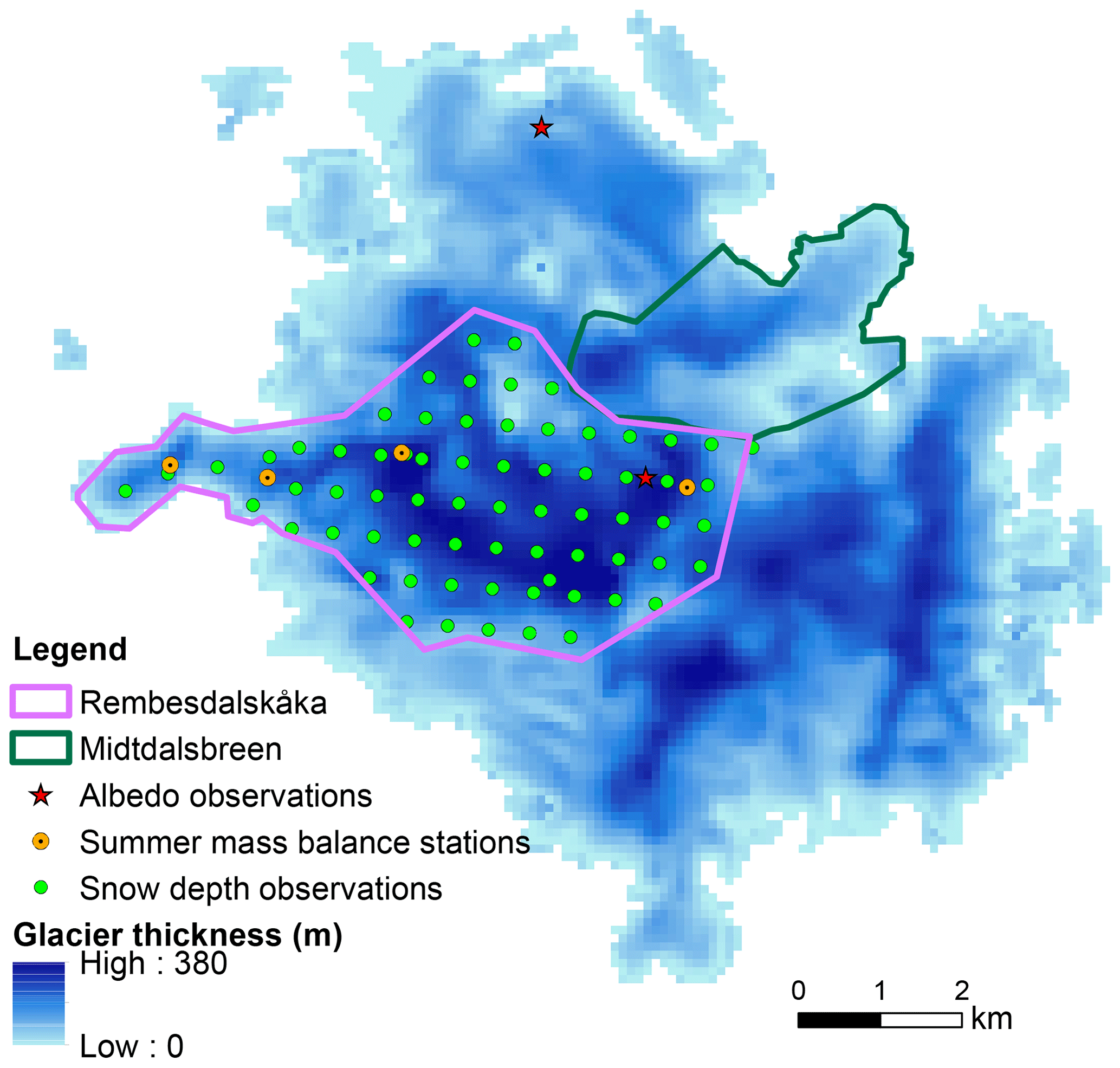
Figure 1Glacier thickness and present extent for Hardangerjøkulen. The outlet glaciers, Rembesdalskåka and Midtdalsbreen, are also indicated. The green dots indicate locations where stake observations for winter balance were obtained, while orange dots indicate location of observations for summer balance. Stars shows location of albedo comparison with model against observations.
In this paper, we present the WRF-Hydro/Glacier system in which Crocus is coupled to the WRF-Hydro model, with the Crocus model representing the glacier. In Sect. 2, we explain the Crocus implementation, while in Sect. 3, we describe the experimental design. In Sect. 4 observational data are discussed. The results are presented in Sect. 5, and finally, conclusions and future work are included in Sect. 6.
2.1 Crocus description and original WRF/Hydro glacier treatment
One of the main reasons to use Crocus for glacier mass balance modeling and the subsequent streamflow modeling is its use of physical parameterization and the ease of implementing non-flowing glacier (ice) layers. By comparison, the Noah-MP has only a maximum of three layers in its snowpack, depending on the total snow depth (Niu et al., 2011). In Noah-MP, the snow albedo option used in this study is calculated based on the snow age through an empirical function. Noah-MP has its own glacier module with the effect that, when there is snow, the Noah-MP snow module is active and albedo is represented by the Noah-MP three-layer snow model, and the minimum albedo of snow is set to 0.55. However, when all snow has melted, the surface is represented by the bare glacier land surface category which has an albedo of 0.675 (0.8 in the visible and 0.55 in the near infrared spectral bands) and roughness lengths and heat conductivity typical for glaciers with old snow. Furthermore, this exposed glacier ice cannot melt as the glacier is only a land surface category (though the glacier is represented in the soil layer with a 2 m layer of water and/or ice but does not provide runoff to WRF-Hydro). Finally, as a result of these limitations in the Noah-MP glacier formulation, the glacier cannot decrease in mass and extent.
Crocus is an energy and mass transfer snowpack model, initially developed for avalanche forecasting (Brun et al., 1989, 1992). In this work, we use the version that was implemented into the French SURFEX model V8.0 (Vionnet et al., 2012). This version has several updates from older versions of Crocus, such as the impacts of wind drift.
The Crocus snowpack model is a multilayered, physically based snow model that explicitly calculates snow grain properties in each snow layer and how these properties change over time. The grain properties of dendricity, sphericity and size are prognosed in Crocus through metamorphism, compaction and impacts of wind drift. Furthermore, the snow albedo is calculated based on the snow grain properties from the top 3 cm of the snowpack (Vionnet et al., 2012) and is calculated in three spectral bands (0.3–0.8, 0.8–1.5 and 1.5–2.5 µm). Impurities in aging snow are parameterized in the UV and visible spectral band (0.3–0.8 µm) from the age of the snow, with a time constant of 60 d. See Vionnet et al. (2012) for a detailed description of the albedo calculations. The albedo over ice is constant in all spectral bands and is 0.38, 0.23 and 0.08 for the spectral bands 0.3–0.8, 0.8–1.5 and 1.5–2.5 µm. The sensible and latent heat are parameterized with an effective roughness length over snow and ice (see Vionnet et al. (2012) for further details). Here we use 1 mm over snow and 100 mm over ice.
In the Crocus model, it is possible to divide the snow into a user-defined maximum numbers of dynamically evolving layers. As new snow is accumulated, a new active layer is added. As different snow layers become similar (based upon the number of user-set layers, the thickness of the snow layers and the snow grain characteristics), these snow layers will merge into single snow layers.
The Crocus module is added to the Noah-MP land surface model in WRF-Hydro to act as a glacier mass balance model. Over designated glacier grid points, the Crocus snow model represents both snow and ice, while outside of the designated glacier grid points, the regular three-layer snow model in Noah-MP is used. Since the current Crocus implementation in WRF-Hydro only acts over designated glacier grid points, we follow Gerbaux et al. (2005) and assume that the temperatures at the bottom of the glacier and the ground below are both at 0 ∘C. Note that we have not yet incorporated fluxes between the glacier and the ground below; thus, there is a constant temperature boundary condition.
Both Crocus and Noah-MP (for the non-glacier grid points) output runoff from snowmelt (and precipitation). This runoff is provided to the terrain routing models in the hydrological model system WRF-Hydro. WRF-Hydro is a model coupling framework designed to link multiscale process models of the atmosphere and terrestrial hydrology (Gochis et al., 2015; Yucel et al., 2015). In the coupled mode, it includes the full functionality of the atmospheric Weather Research and Forecasting (WRF) modeling system. WRF-Hydro enables the simulation of land surface hydrology and energy states and fluxes at high spatial resolutions (typically 1 km or less) using a variety of physics-based and conceptual approaches (Yucel et al., 2015; Senatore et al., 2015). It contains horizontal routing processes and water management modules and is linked to the Noah-MP land surface module (among others). The added capability of running Crocus as a glacier mass balance module in WRF-Hydro is called the WRF-Hydro/Glacier system from here onward.
Note that our implementation of Crocus as a glacier mass balance model does not address glacier movement (i.e., plastic flow) nor lateral wind (re)distribution of snow. Being a relatively flat dome glacier, the Hardangerjøkulen glacier that we focus on here does not move much in a year, and therefore, the lack of dynamical movement of the glacier is not expected to have a major impact on the results in this paper, as we only consider 4 simulation years. On the other hand, the lateral snowdrift and wind-driven redistribution of snow on Hardangerjøkulen can be significant, and our results are likely impacted by the lack of this physical process in the model. It is worth mentioning that including lateral movement of snow due to snowdrift in the model system is not a trivial task, and it is, therefore, not currently included. However, there are two options for including impacts on the snow due to wind. One of the options impacts the snow density during blowing snow events (Brun et al., 1997). This option is important in polar environments (Brun et al., 1997), and we found it necessary in our simulations as well. The other option is the sublimation due to snow drift, which was implemented by Vionnet et al. (2012) and which is in the Crocus version that is used in this study. This option was also crucial to include in order to accurately simulate the glacier mass balance over Hardangerjøkulen. It is especially important for reproduction of the observed heterogeneous snow distribution.
2.2 Initialization of glacier module in WRF-Hydro/Glacier
To run the WRF-Hydro/Glacier system, the glacier to be evaluated must be initialized with its thickness and extent. Here we focus on the Hardangerjøkulen; its extent and height were obtained from the NVE (Melvold et al., 2011). Figure 1 shows the glacier thickness and extent of Hardangerjøkulen at 100 m grid spacing (for which the entire WRF-Hydro/Glacier model is run). At initialization, it is assumed that the glacier consists of only ice, and the density is that of pure ice (900 kg m−3). In the simulations presented here, the user-defined maximum layers are set to 40 layers, and the glacier is initialized with all the layers having the same assumed density and snow grain properties. As new snow accumulates during the simulations, the layers representing the glacier will start to merge since all 40 layers contain the initialized ice. Here, the thickest parts of the glacier merged to an average of eight layers after 5 months of simulation and remained fairly constant for the remainder of the simulation. Revuelto et al. (2016) also used Crocus for surface mass balance studies. They initialized their glacier with the same glacier thickness (40 m) over the entire glacier and in the six lowest layers, with the thickness progressively increasing with depth. In contrast to this study, they reinitialized the glacier to 40 m every new season (1 August) so that the glacier would not decrease in extent, while here the glacier is only initialized once at the beginning of the simulation with the observed glacier thickness.
As implemented, if the glacier completely melts over a user-defined glacier grid point, the original Noah-MP module is used from this point on. Therefore, as currently implemented, the glacier cannot grow horizontally in extent; it can only decrease in extent, as no dynamic response of the ice mass is included in the model. Over short model time periods, the lack of increase in glacier extent might impact a few grid points at the edges of the glacier. However, given the expected increase in temperature in the future, we do not expect that limiting glacier horizontal growth will have a major impact over most studied glaciers as most are likely to decrease in mass and extent.
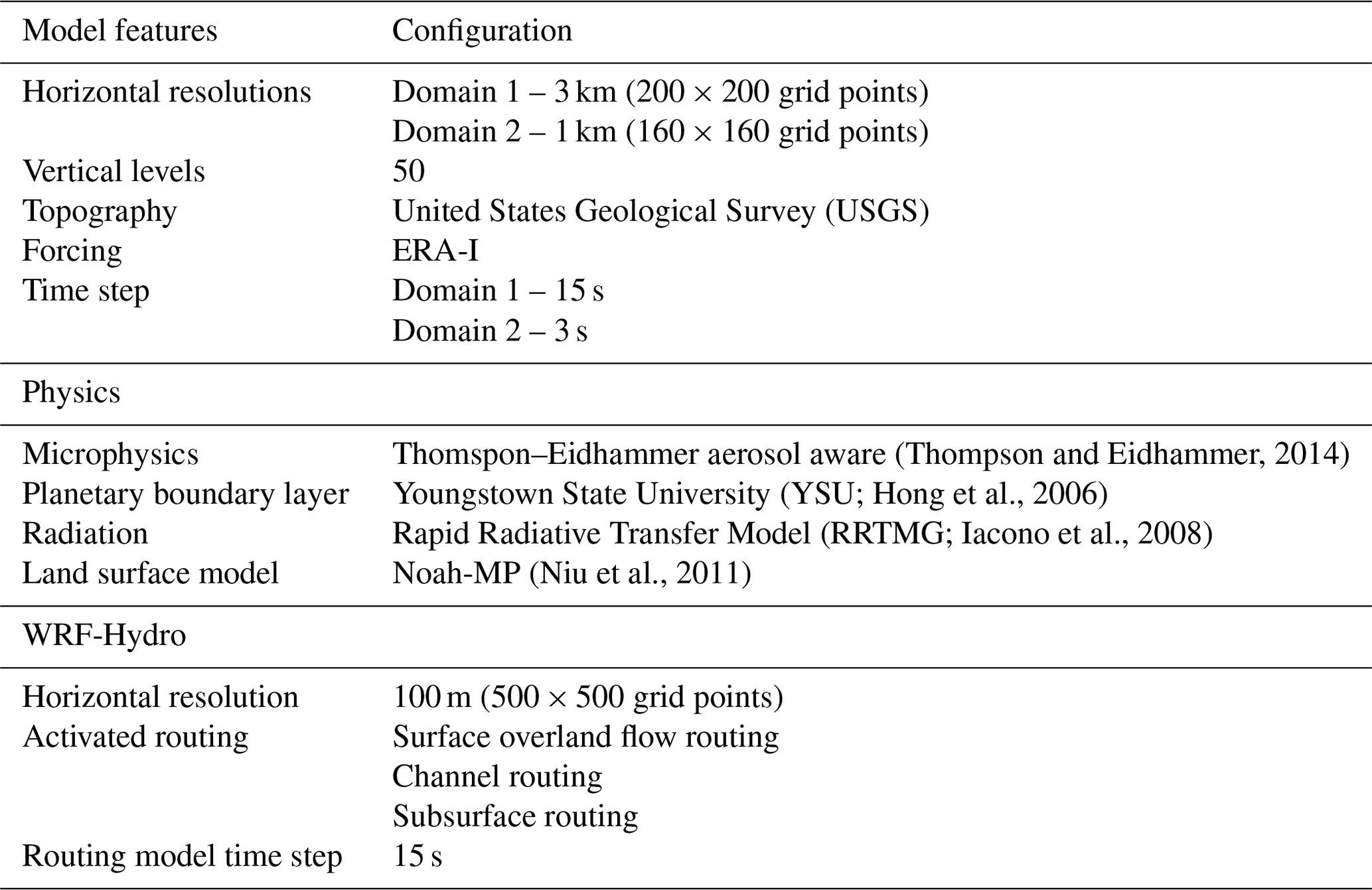
For meteorological input data to the WRF-Hydro/Glacier system, dynamically downscaled data from the WRF model version 3.9 (Skamarock et al., 2008) were created over southern Norway. WRF was run with an outer domain (Domain 1), with a 3 km grid spacing, and an inner domain (Domain 2), with a 1 km grid spacing (see Fig. 2, top), with 51 stretched vertical levels (the lowest prognostic level is 25 m). The ECMWF Re-Analysis Interim (ERA-I) data set was used for input and boundary conditions, and the model was run from 1 August 2014 to 1 January 2019. The microphysics scheme used was the Thompson–Eidhammer aerosol-aware scheme (Thompson and Eidhammer, 2014), the Yonsei University (YSU, Hong et al., 2006) scheme for the boundary layer (Hong et al., 2006), the rapid radiative transfer model (RRTMG) for longwave and shortwave radiation calculations (Iacono et al., 2008) and the Noah-MP land surface model (Niu et al., 2011). See Table 1 for the configuration.
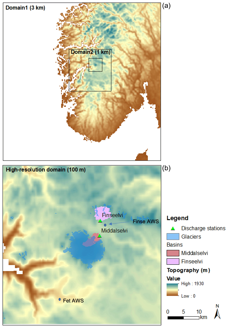
Figure 2Model domains. Panel (a) shows the WRF domains with 3 and 1 km grid spacing. Panel (b) shows the high-resolution domain (100 m grid spacing) used with WRF-Hydro/Glacier. Furthermore, the outline of Hardangerjøkulen and the river basins of the two rivers with discharge observations are included as well.
We did not use any lake models; thus, in WRF, the skin temperature of lakes is typically set to the same temperature as the nearest grid point that is defined as sea surface. With this setting, the lakes will not reach freezing temperatures since the oceans surrounding southern Norway typically do not freeze in the winter. To rectify this problem, we assign a 10 d moving average skin temperature from the associated ERA-Interim grid point onto the lake grid points to allow a representation of freezing lakes. The fjords still use the sea surface temperature from ERA-Interim. We acknowledge that a large step from ∼75 km (ERA-I) to 3 km in WRF is of concern. However, we follow the findings by Liu et al. (2017), where they state, “Tests showed that one-way nesting WRF, at 4 km grid spacing, with the ∼75 km reanalysis, was an adequate configuration without the need for a coarse grid that intermediates the ERA-Interim data and the WRF domain”. What is important is that the area of interest must be sufficiently large enough for mesoscale spin up. Our domain of interest (Domain 2) is slightly closer to the boundary than what is in Liu et al. (2017). However, as shown below, the model results are quite reasonable; thus, we believe that the jump from ∼75 to 3 km is adequate.
The 1 km WRF (inner-nest) simulation results are used as input to run WRF-Hydro/Glacier. The WRF-Hydro/Glacier domain has 100 m grid spacing (Fig. 2; bottom) and covers a smaller area compared to that of the 1 km domain. The precipitation, 2 m temperature, 10 m wind speed, 2 m water mixing ratio, surface pressure and long and shortwave radiation outputs from the WRF 1 km simulations were bilinearly regridded to the 100 m grid spacing in the high-resolution domain. We note that we did not account for variability in terrain in the regridding process. Thus, the atmospheric forcing is still “smooth” with regards to a 100 m grid. However, the region of interest (Hardangerjøkulen and surrounding terrain) is an open, mostly flat area, and we, therefore, believe that, for this specific case, disregarding the variation in terrain does not have much impact on mass balance calculations. To partition the rain and/or snow from the input precipitation, WRF-Hydro/Glacier use the rain and/or snow partition from Jordan (1991). The streamflow routing is run at the same resolution as Crocus (i.e., at 100 m). Finally, no calibrations were applied to the routing model.
Hardangerjøkulen is a well-observed glacier with several decades of mass balance observations and several field campaigns. In the following, data from field observations, the ongoing mass balance observations and remote sensing are used to evaluate the WRF-Hydro/Glacier system.
4.1 Glacier mass balance
Glacier mass balance is the amount of mass a glacier gains or loses over a year (sum of accumulation and ablation). NVE has gathered winter, summer and annual (net) mass balance (winter plus summer mass balance, where summer mass balance is negative) observations over Rembesdalskåka since 1963 (e.g., Andreassen et al., 2020), where Rembesdalskåka is the west/southwest glacier outlet of Hardangerjøkulen (see Fig. 1). The observations are gathered at several locations on the glacier, from the lower to the upper parts (1066–1854 m a.s.l.), by using stakes (aluminum poles inserted into the glacier) and in spring, by probing (using thin metal rods to measure snow depth) to the previous year's summer surface. Winter mass balance is found from the observed snow depth (by stakes and rod soundings at approximately 60 locations; see Fig. 1) and from snow density measurements at one location on the glacier. To determine summer balance (at four locations), the observations are usually conducted at the end of the main melt season around the time period of September–October, while the winter balance is usually determined at the end of the accumulation season in May–June. Often summer balance observations are conducted when new snow has accumulated on the upper part of the glacier. However, the summer surface can be identified in shallow snow pits. Therefore, to determine mass balance from the WRF-Hydro/Glacier simulations, we use the date with the smallest simulated glacier mass to determine the end of the summer and start of the winter season instead of using the actual date for when observations were gathered. Details about the annual mass balance observations are found in the NVE report series Glaciological investigations in Norway (Kjøllmoen et al., 2016, 2017, 2018, 2019).
4.2 Radar-derived snow thickness
Variations in snow accumulation were measured over Hardangerjøkulen in April 2017 and 2018, using ground-penetrating radar (GPR). In 2017, surveys were conducted with a MALÅ geoscience GPR system. In 2018, this system was not available; hence, a Sensors & Software Inc. pulseEKKO PRO model was used instead. However, data from these two systems are directly compatible since both were acquired with antennas of 200 MHz center frequency. The GPR systems were towed behind a snowmobile at ∼15–20 km h−1. The interval between successive GPR recordings is ∼0.2 s, giving a distance sampling interval of ∼1 m (regularized to exactly 1 m in processing). A GPS system was also mounted on the snowmobile, recording positions every 1–2 s, to locate the GPR recordings. The positional accuracy of the GPS is ∼5 m. A total of 116 and 27.4 km of measurements were acquired in 2017 and 2018, respectively, and both acquisitions featured numerous crossing points, such that the internal consistency of accumulation estimates could be ensured.
GPR systems record the travel time of a radar pulse through the ground; therefore, estimates of winter accumulation require some measure of the GPR propagation velocity to covert time to depth. This was obtained using so-called common midpoint (CMP) data (e.g., Booth et al., 2011, 2013), in which GPR responses suggested an average velocity of 0.218±0.001 m ns−1 for the upper ∼2.8 m of the snowpack. With no other velocity control available, this value is applied to convert all GPR travel time estimates to a snow depth.
The base of winter snow accumulation was taken to be the first prominent reflective horizon within the GPR record. This is straightforward in the Hardangerjøkulen ablation zone, typically at elevations m, where winter snow directly overlies the glacier surface, typically at a depth of 2–3 m. Here, the only significant reflection is from the glacier surface itself. Consequently, depth errors are expected to be less than ±0.1 m. However, areas of firn accumulation have a more complex pattern of reflectivity, and it is not always possible to guarantee accurate snow thicknesses, and errors here may be up to ±1 m. However, given the crossing points in the GPR records, depth estimates are at least internally consistent, and errors are expected to vary systematically across the entire record.
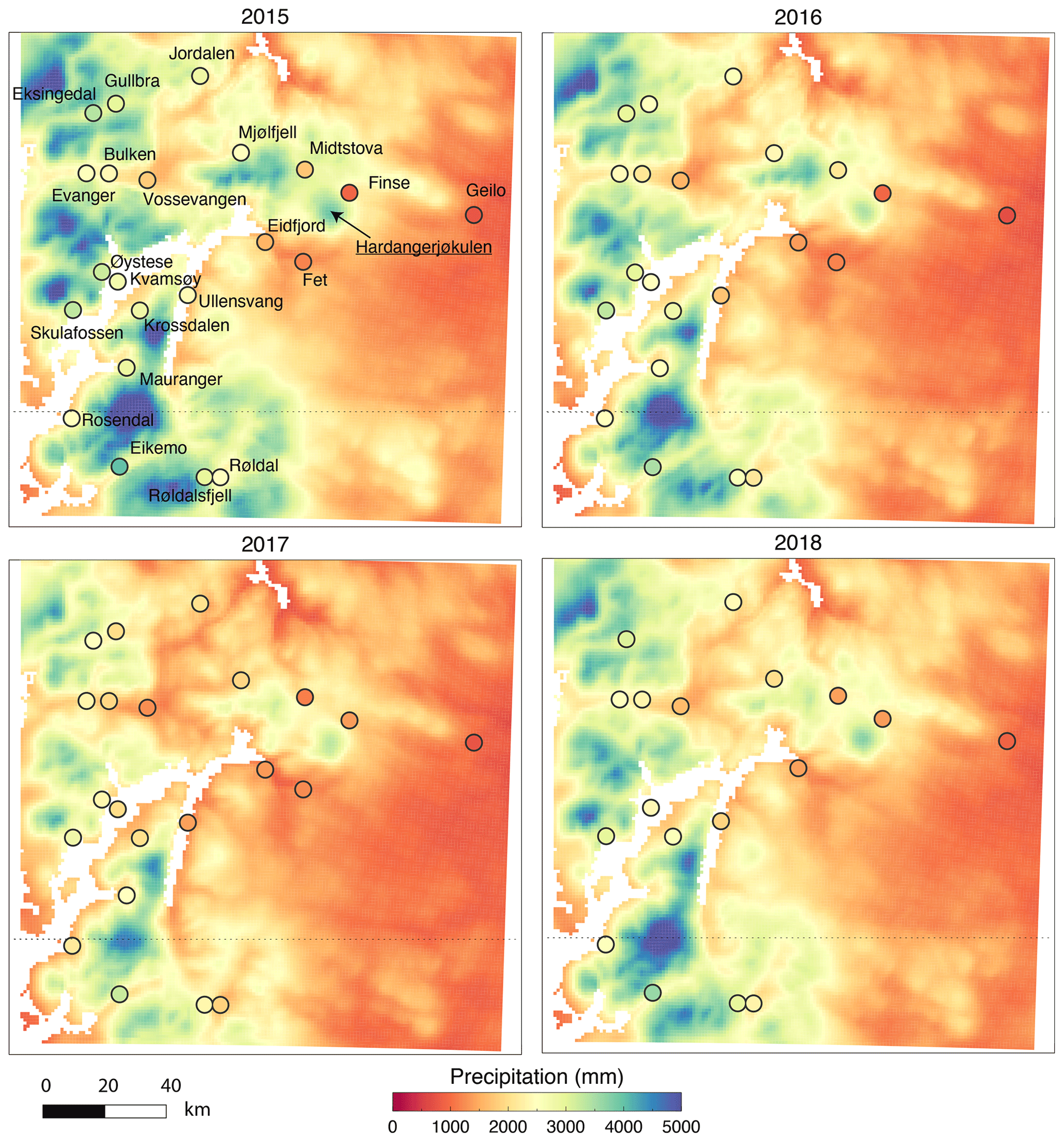
Figure 3Simulated and observed precipitation (October–September) for mass balance years 2015–2018. Circles represent observations from automated weather stations (AWSs). The location of Hardangerjøkulen is also indicated.
4.3 Moderate Resolution Imaging Spectrometer (MODIS) snow albedo
The Crocus model computation of snow albedo depends on the physical properties of the snow grains, while the formulation used by Noah-MP model uses only a time-dependent empirical formulation. To evaluate the modeled snow albedo, we use the NASA Moderate Resolution Imaging Spectrometer (MODIS) daily snow albedo product version 6 from Aqua (MYD10A1; Hall and Riggs, 2016) and Terra (MOD10A1; Hall and Riggs, 2016). These products are reported with 500 m grid spacing.
4.4 Streamflow
Discharge measurements were obtained at two rivers. One river (here named “Middalselvi”) is fed by meltwater from the Midtdalsbreen (a glacier arm of Hardangerjøkulen), where the catchment is about 12 km2 and 60 % glacierized (see Fig. 2). The other river is Finseelvi, where the catchment is about 16 km2 and 14.7 % glacierized and not much impacted by glacier melt. A total of two HOBO water level loggers were installed in each catchment in the fall of 2016, and we have data until November 2018.

Figure 4Percent difference in simulated and observed precipitation at all stations for mass balance years 2015–2018. Some values above Midtstova and Finse are above the axis limit and are therefore indicated with labels.
5.1 WRF stand-alone verification
The WRF model simulations were validated by using observations from 21 automated weather stations (AWSs) operated by the Norwegian Meteorological Institute (Fig. 3). These data were compared to the output of the 1 km simulations (Domain 2). The locations of the stations are given in Fig. 3 (top left panel), along with the location of Hardangerjøkulen. We note that additional stations exist in the southwestern corner of the domain that were excluded in our evaluation because they were too close to the border of the domain. Figure 3 shows the total precipitation for the mass balance years 2015, 2016, 2017 and 2018, with observations given as colored circles. Here we define a mass balance year from 1 October in the previous year through 30 September of the current year. For example, the mass balance year 2015 ranges from 1 October 2014 to 30 September 2015. As can be seen in Fig. 3, the model captures the spatial precipitation distribution of the observed precipitation, with maximum precipitation near the coast and minimum to the lee of the mountains. The locations of some of these observations are in or near narrow fjords, such as the Ullensvang, Eidfjord, Skulafossen, Kvamsøy and Øystese stations. These locations tend to underpredict precipitation by nearly 20 % (see Fig. 4), which is a larger bias than stations further away from the fjords. The values shown in Fig. 4 are obtained by finding the closest grid point to the actual location and then, from there, taking the four closest model grid points relative to the selected grid point closest to actual AWS elevation. Furthermore, stations that are located in the model over 100 m above the actual elevation are not included. Of the stations, three (Finse, Midtstova and Geilo) are located at high-altitude, exposed locations. At these stations, there is a large undercatch of observed snow in the wintertime when the snow can blow past the precipitation gauges instead of falling into the gauges (Rasmussen et al., 2012). The stronger the wind, the larger the undercatch. The data obtained from the Norwegian Meteorology Institute for these stations have not been corrected for any undercatch. Figure 5 shows the effect of undercatch of snow at Finse, which is the station that is located closest to Hardangerjøkulen, about 4 km north–northeast of the edge of Midtdalsbreen and about 11 km from Rembesdalskåka. In Fig. 5, the accumulated precipitation and temperature for the 2016 summer and winter season is shown at both Finse, Fet (a station about 25 km southwest of Finse but about 14 km away from Rembesdalskåka) and Evanger (a nonexposed inland station with little snow). Similar results are seen for 2015, 2017 and 2018 (not shown). As can be seen, WRF compares well with observations at Evanger and Fet for almost the entire period (Fig. 5a–d). WRF precipitation also compares well with observations at Finse in the summer season (Fig. 5f) but has much more precipitation than the observations in the winter season (Fig. 5e), where wind speeds are often more than 5 m s−1 (Fig. 5i) and temperatures are below freezing. Furthermore, WRF does simulate the storm sequences well, as seen in Fig. 5g and h. Thus, we attribute the low observed precipitation compared to WRF during the winter season at Finse to the undercatch problem, as precipitation modeled at Fet compares very well with observations. Note that, during 17 to 26 September, the Finse station did not provide any data (Fig. 5f, h and j). However, during this time period, WRF did not predict any precipitation, and Fet did not observe any precipitation. Thus, the cumulative precipitation shown in Figure 5f is still valid.
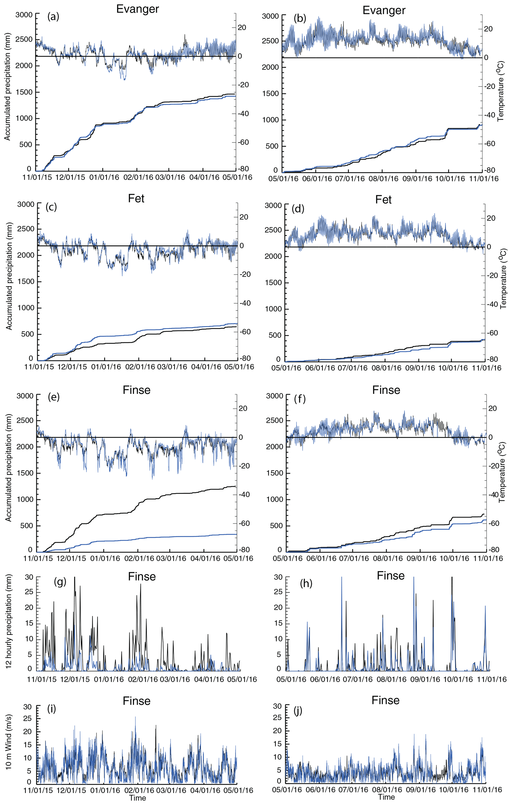
Figure 5Observed (blue) and modeled (black) accumulated precipitation and temperature at Evanger (a, b), Fet (c, d) and Finse (e, f) stations for the 2016 winter season (a, c, e, g, i) and 2016 summer season (b, d, f, h, j). Panels (g) and (h) show the time series of precipitation. The bottom panels (i, j) show the 10 m wind speed at Finse.
The World Meteorology Organization (WMO) Solid Precipitation Intercomparison Experiment (SPICE) was set up to evaluate the undercatch of snow and develop transfer functions to correct for the undercatch of solid precipitation (Smith et al., 2020). One location for these studies is Haukeliseter, which is about 20 km from Røldal (see Fig. 2) and is within the 1 km domain. In these studies, several different precipitation gauges and wind shield combinations were used. The Double Fence Automated Reference (DFAR) was deployed as the reference and is used as the “truth” precipitation. We compared the WRF model results with the DFAR data (Smith et al., 2019), and WRF is predicting more precipitation compared to these observations, with a bias typically at ∼30 % (not show). About 10 % of this bias could potentially be attributed to underestimation with the DFAR (Rasmussen et al., 2012). Compared to what is found at locations with little impact of snow, the bias in WRF is opposite and higher. With regards to transfer functions (correcting for under catch in observations), Smith et al. (2020) stated this in their study: “Although the application of transfer functions is necessary to mitigate wind bias in solid precipitation measurements, especially at windy sites and for unshielded gauges, the inconsistency in the performance metrics among sites suggests that the functions be applied with caution”. We are, therefore, not adjusting the observed observations on Finse for our evaluation and rather stressing the good comparison between model and observations at Fet and summer season precipitation on at Finse.
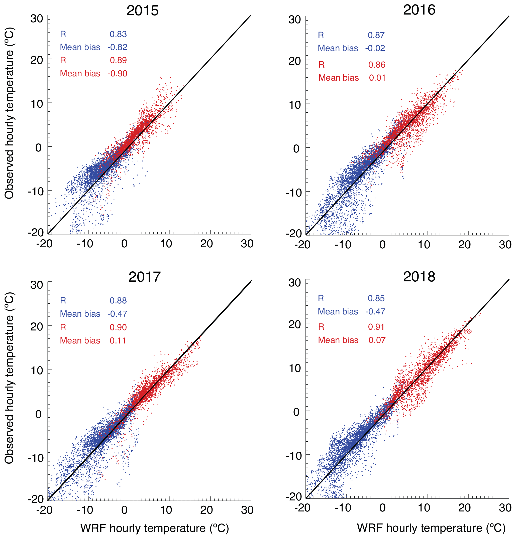
Figure 6Scatterplot of observed and simulated temperature for mass balance years 2015–2018 at Finse station. Blue represents the winter season, and red represents the summer season.
We conclude, as shown above, that most of the nonexposed inland stations are relatively well simulated by the WRF-model, and the seasonal cycle of precipitation is captured. We note, however, one time period where WRF is underpredicting the precipitation relative to locations near Finse (Hardangerjøkulen). Several stations near Finse do not catch a precipitation period in the middle of January 2017, which has an impact on Finse as well. This underprediction in WRF is difficult to directly evaluate at Finse, but the two stations near Finse (Fet and Eidfjord) clearly have an underprediction at this time period (not shown). We note that the observed storm sequences were captured in the simulation, and the wind direction was well simulated, as was the wind speed during this precipitation event (not shown), just not the precipitation amount. The effect of this precipitation time period will be discussed in relation to the mass balance and streamflow results is Sect. 5.
Figure 6 shows a scatterplot of observed and simulated 2 m temperature at the Finse AWS. As can be seen, the modeled temperature compares well with the observed but with a small negative bias in the winter. At the very low observed temperatures ( ∘C), WRF often has a positive bias. This is likely due to WRF not capturing the strong inversions that often occur in the winter months (Mölders and Kramm, 2010; Hines et al., 2011). Figure 5e also shows this positive bias at the very low temperatures. However, in general, WRF compares well with observations with a correlation coefficient near 0.9.
Figure 7 shows the simulated and observed 10 m wind speed and direction for the entire simulation period at Finse. Although the wind direction is not an input variable in the land surface model in WRF-Hydro/Glacier, the wind direction can dictate the precipitation amount and type; thus, wind direction is important for obtaining correct simulation of precipitation and subsequent glacier mass balance. As can be seen, the simulated wind direction compares well with the observed. Mean bias is −0.13 m s−1, and the coefficient of correlation is 0.8. Overall, the major simulated wind directions and speed are simulated quite well (also see Fig. 5 for wind speed).
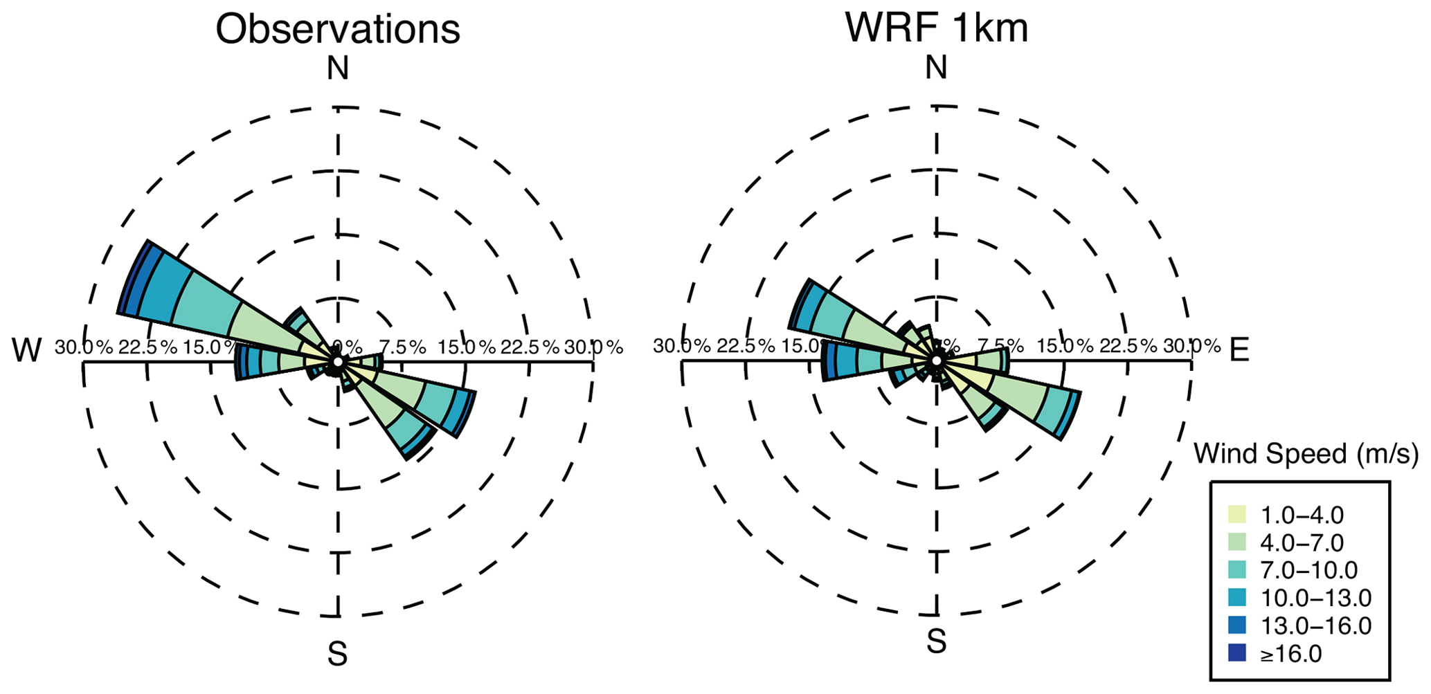
Figure 7Wind rose of simulated and observed 10 m wind speed and direction at Finse AWS stations for the entire simulation period.
5.2 Glacier mass balance and snow height
Figure 8 shows the observed glacier mass balance, new accumulated snow thickness and density from NVE versus modeled for the 2015–2018 mass balance years for Rembesdalskåka. The observed winter balance is taken from the green locations shown in Fig. 1, while the summer balance is found at the four red locations in Fig. 1. The observed mass balance is plotted as averages in intervals of 50 m. For the summer balance all values between the four locations are interpolated. The modeled winter (and summer) balance is plotted as averages of all grid points over Rembesdalskåka within intervals of 30 m. As can be seen, the modeled mass balance (winter, summer and net; Fig. 8a, d, g, and j) is generally comparable with the observations. The observed winter mass balance shows a small decrease at the top of the glacier, with a slight increase about 200 m below the top (see left panels). This is most likely due to the redistribution of snow that is common at Finse and its surroundings, as strong winds occur often there. Since lateral redistribution of snow is not included in the Crocus and Noah-MP models, the modeled mass balance increases more linearly towards the top compared to the observations. The winter mass balance is about 29 % (20 %) underestimated in 2017 by Crocus (Noah-MP), which is likely due to the underprediction of winter precipitation at Finse and nearby stations in this year (discussed in Sect. 3.1). For the 3 other years (2015, 2016 and 2018), the modeled winter balance is within 9.3 %, 13.8 % and 5.1 % (8.7 %, 14.7 % and 2 %) of the observed winter mass balance for Crocus (Noah-MP), respectively (see Fig. 9). The reason for the slightly larger bias for Crocus is not known at this point. However, note that Crocus matches better with the observations at lower levels below about 1500–1600 m in 2017 and 2018 (see Fig. 8; left and middle panels). This does not appear in the total mass balance comparisons since most of the mass is above 1600 m due to higher snow thickness and larger area (see Rembesdalskåka; Fig. 1). Another point to add here is the improved simulation of winter mass balance of Rembesdalskåka compared to Engelhardt et al. (2012). They used gridded interpolated precipitation data from seNorge (http://senorge.no, last access: 14 June 2021) and obtained a mean negative bias of 28 % from 19 modeled winter mass balance years for Rembedalskåka, while we use high-resolution, regional-scale modeling to obtain horizontally distributed precipitation.
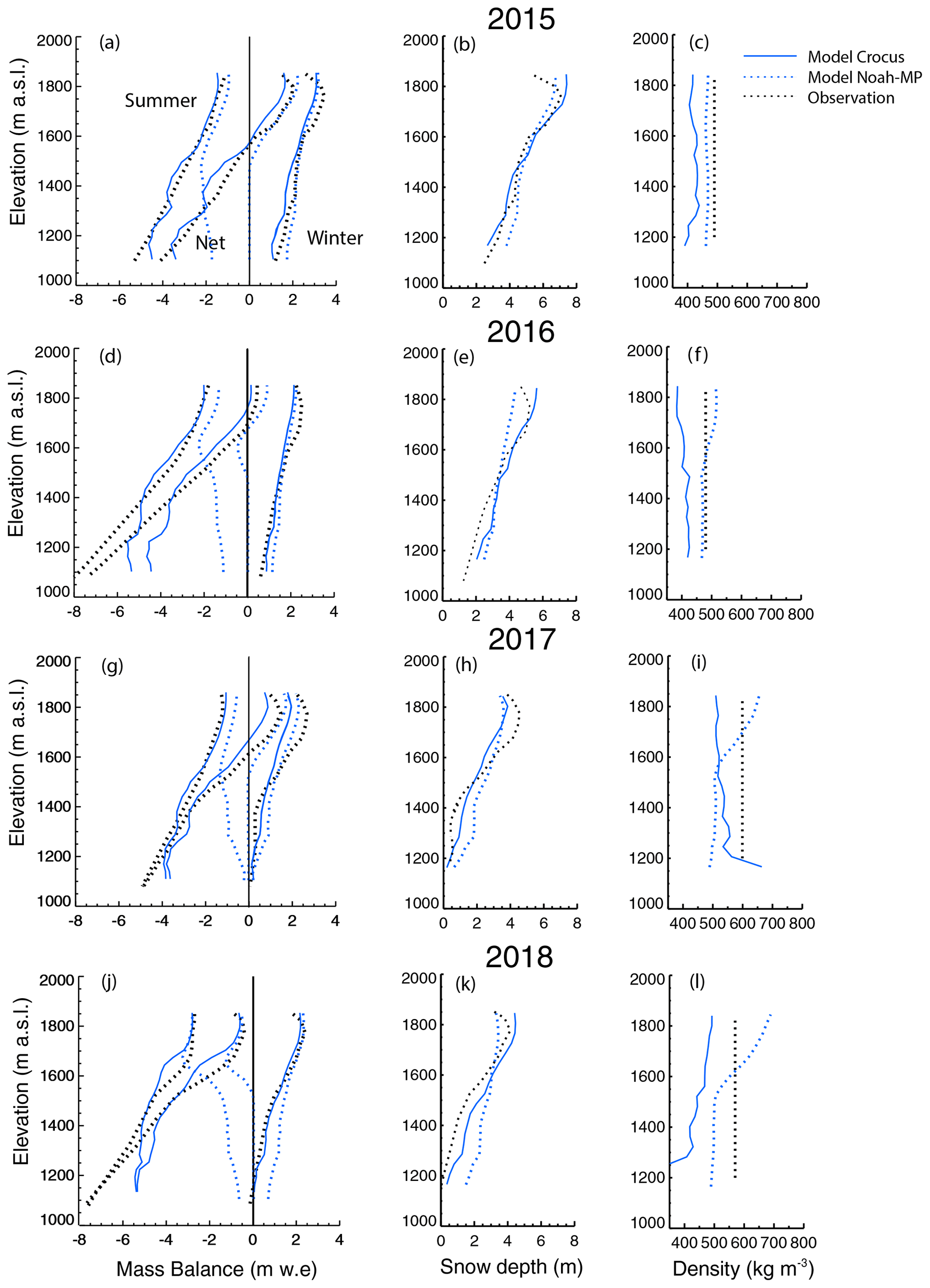
Figure 8(a, d, g, j) Mass balance across Rembesdalskåka with height. (b, e, h, k) Accumulated snow thickness associated with the winter mass balance. (c, f, i, l) Snow density of the accumulated snow. Each row represents a different year.
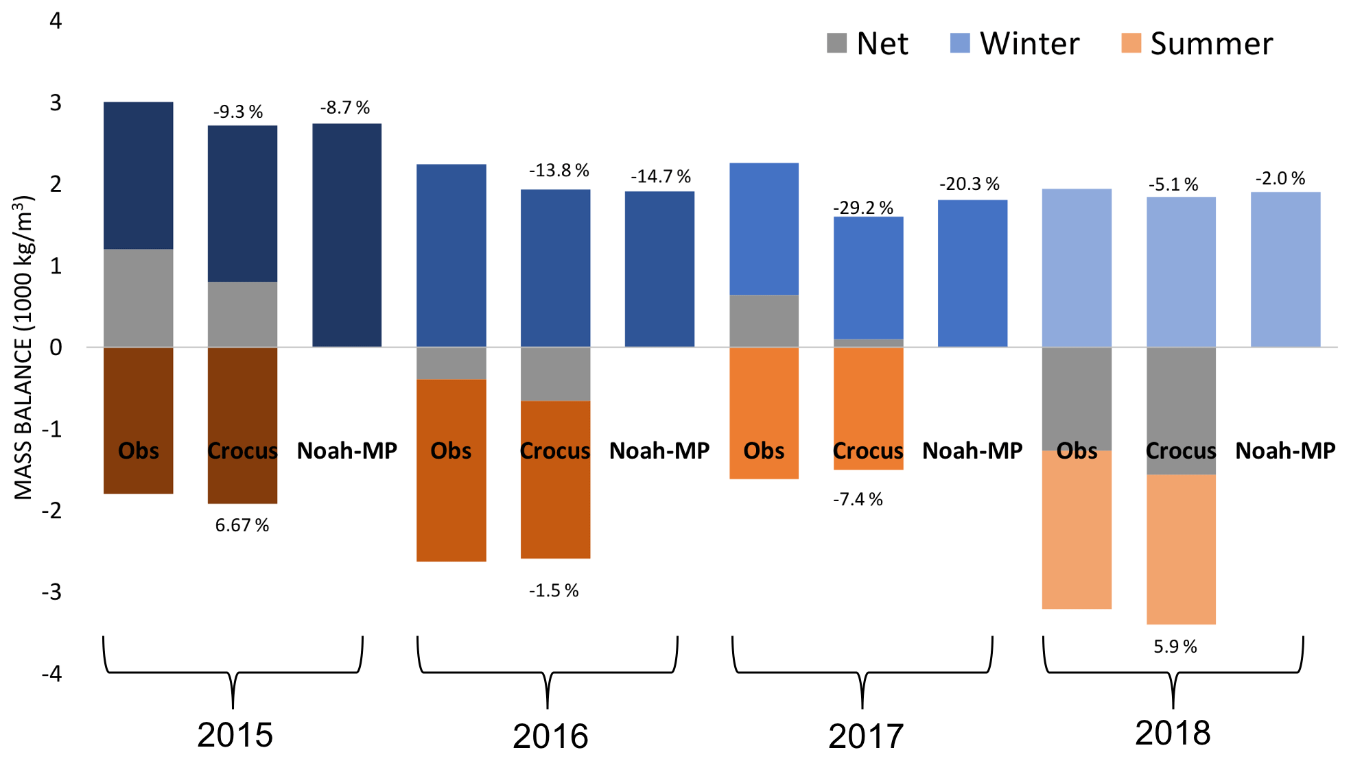
Figure 9Box plot of winter, summer and net balance for the mass balance years 2015–2018 for Rembesdalskåka. Only winter mass balance is shown for Noah-MP.
For the summer and net mass balance, we only consider Crocus since Noah-MP cannot melt more than the accumulated snow amount from the model start (see Fig. 8; left panels). As the winter balance, the modeled summer mass balance is also in general agreement with the observations, with a bias of 6.67 %, −1.5 %, −7.4 % and 5.9 % in 2015, 2016, 2017 and 2018, respectively (Fig. 9). However, the modeled 2018 summer balance curve in Fig. 8j shows a different function of height compared to the observations with stakes. This year the summer balance observations by NVE were taken late in the fall (22 November), while the actual minimum was most likely in September, based upon our model results. At this point, only the two top stakes that are used to determine mass balance were left standing, and both were located above 1750 m, while the other sakes had melted out (Kjøllmoen et al., 2019). Our model results compare favorably at the top altitudes where observations were available. Below ∼1750 m, there are no observations, and observed summer mass balance is, instead, estimated from observed temperatures at nearby stations and the relationship between temperature and melting for the period 2012–2017 (Andreassen et al., 2020). Therefore, there is a possibility that our model results are closer in agreement to the actual melting than what is indicated in Fig. 8j.
The modeled distribution of snow thickness and snow water equivalent (SWE) over Rembesdalskåka is comparable to measurements by NVE (Fig. 10). The NVE data are the same as that used in Fig. 8, while they are not averaged in elevation transects as in Fig. 8. There is more heterogeneity in the observations, as would be expected, since the model does not account for lateral redistribution of snow. Despite this, Crocus does account for sublimation of snow drift, which results in more heterogeneity in the spatial snow distribution over the glacier compared to Noah-MP. The relatively large underestimation of modeled SWE (i.e., the winter balance) in 2017 is also seen in the snow thickness. This is also evident in Fig. 8 (middle panel), which shows the snow depth as a function of altitude. The simulated snow depth for 2015, 2016 and 2018 compares better with observations at altitudes above 1600 m compared to the mass balance simulations (Fig. 8; left panel).

Figure 10Mass balance at Rembesdalskåka. The two leftmost columns show the winter mass balance and accumulated snow height across Hardangerjøkulen as modeled with Crocus. Colored circles are observations from NVE. The two rightmost panels are the same as the two leftmost panels but as modeled with Noah-MP.
The observed densities for which the observed mass balance is based upon are 490, 481, 599 and 576 kg m−3 for the years 2015–2018, while the modeled Crocus snow densities, on average, are lower (see Fig. 8; right panel). Snow densities from Noah-MP are also lower but higher than the Crocus snow densities. In the first modeling year of 2015 (Fig. 8c), the snow density with Noah-MP is uniform over all elevations. However, as the simulations continued over several seasons (Fig. 8f, i and l), the snow density increases with height for the following years. The reason for this increase is that Noah-MP only has three model layers. When new snow accumulates in the winter, some of this snow is merged with higher density multiyear snow from previous years in the accumulation zone of the glacier. It is, therefore, difficult to estimate the actual modeled snow density of the new seasonal snow layer in the accumulation zone with Noah-MP in a multiyear simulation. The underestimation of density with Crocus is in agreement with Quéno et al. (2016), who found that the bulk density in their study using Crocus also was underestimated, and that Crocus tends to underestimate the snow compaction. On the other hand, since the density used to approximate the observed mass balance is taken from only one location, there are likely some uncertainties in the representability of this density over the entire glacier.
Ground-penetrating radar observations were gathered in April 2017 and 2018. Note that this time period is not the same as when the winter mass balance is determined with stake observations which occurred at the end of or after the accumulation season (Fig. 10). Figure 11 shows both modeled and observed spatially distributed accumulated snow for the respective winter season, and the snow depth as a function of height. Figure 12 shows a 2-D histogram of the same data. Although these data show some scatter, and isolated observations significantly diverging from the model output (blue), the occurrence of such points is between 10–100 times lower than those which plot close to the one-to-one comparison (red). As such, the majority of depths observed within the GPR data set match the model outputs to within 1 m. Crocus has more variation in snow depth over the glacier compared to Noah-MP (see Fig. 12), but the modeled glacier in both snow models has less heterogeneity compared to the observations (Fig. 11). For 2017, we can see that there are areas over Rembesdalskåka where the model clearly underestimates the snow thickness, as can also be seen with the point observations from NVE in Fig. 10. However, at other locations on Rembesdalskåka, the comparison is favorable. Also, in the northern and western part of Hardangerjøkulen (the entire glacier complex), the model matches the observed snow thickness quite well. In the middle part of the glacier, Crocus estimates deeper snow depth compared to Noah-MP and is closer in agreement with the observations both in 2017 and 2018. The reason for the lower snow depth in Noah-MP is likely due to the high snow density at higher elevations (see Fig. 8).
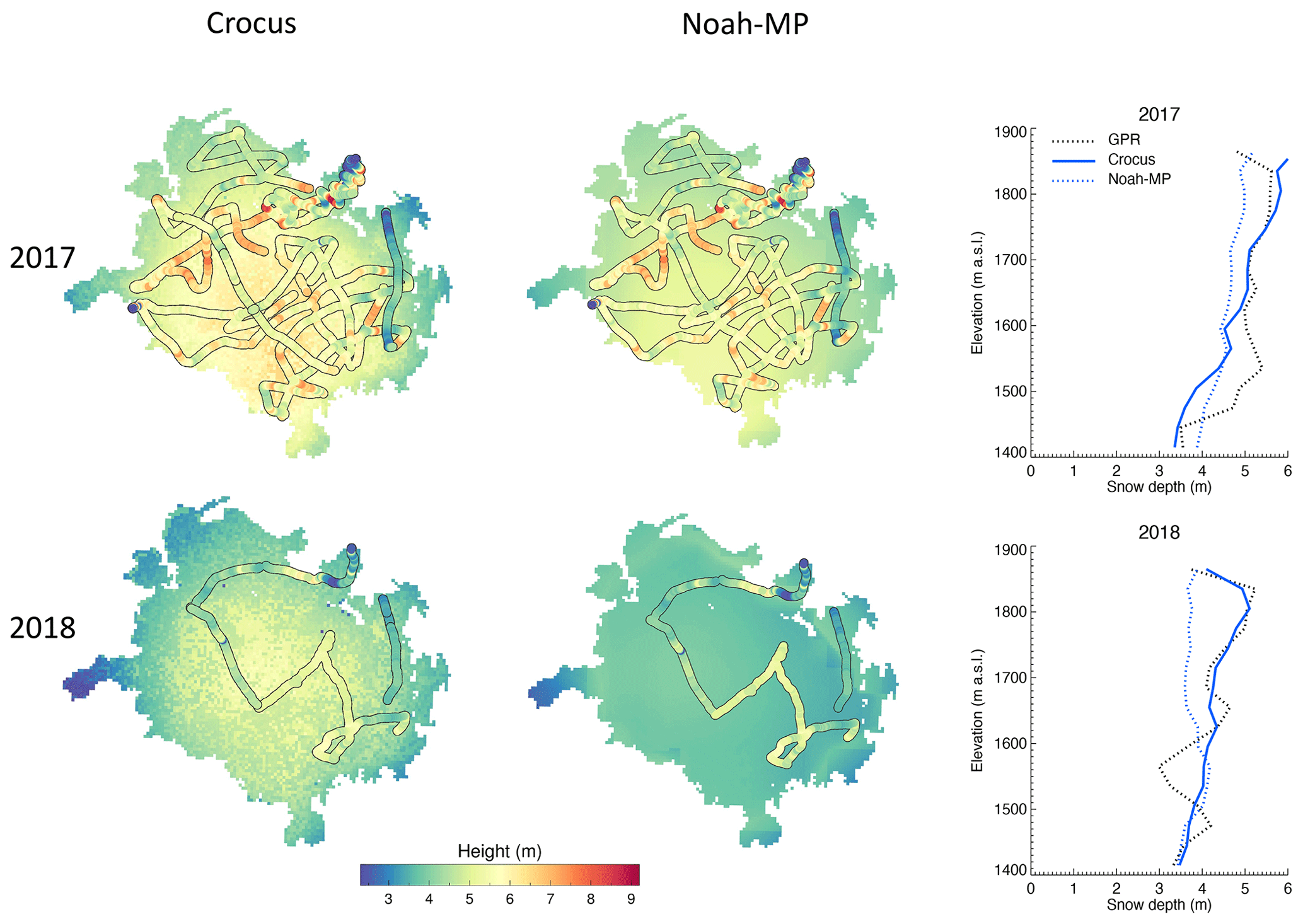
Figure 11Modeled and observed snow accumulation in April. Observations are with ground-penetrating radar. The left plots are the simulation results with Crocus, and the middle plots are simulation results with Noah-MP. The rightmost plot shows the snow depth as a function of elevation.
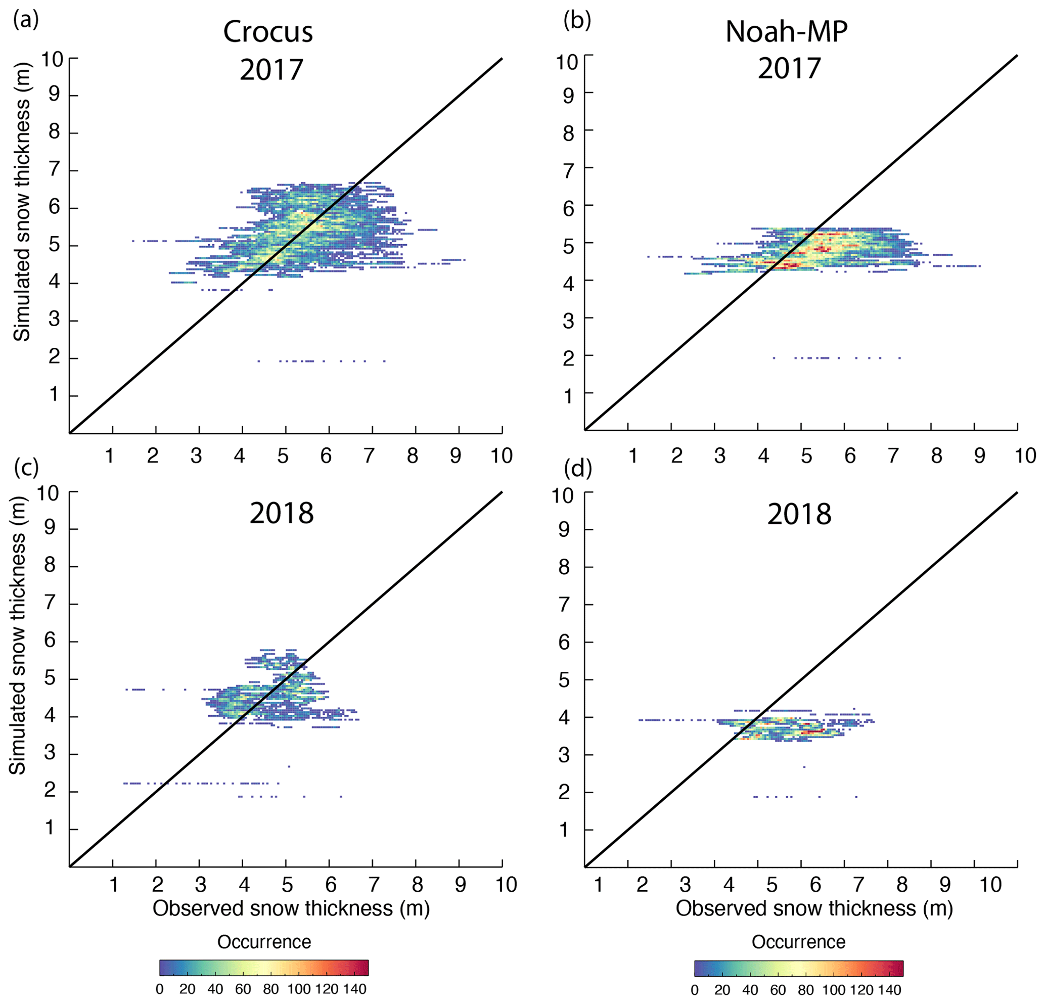
Figure 12Scatterplot of modeled and observed snow accumulation. The observations are with ground-penetrating radar. Panels (a, b) are simulation results with Crocus, and panels (c, d) are simulation results with Noah-MP.
In Sect. 2.1, we mentioned the importance of adding sublimation of blowing snow in our simulations. Figure 13 shows the snow thickness and the respective scatterplot for when the sublimation of blowing snow is not included (which is the default in the SURFEX V8.0 setup when downloaded). As can be seen, the simulated snow thickness is slightly higher than the observations with the GPR, and this is especially true at the eastern part of Hardangerjøkulen. During the 2017 winter season, this region had, on average, the strongest winds, causing more sublimation from snowdrift than at other locations on the glacier. Without including sublimation of blowing snow, the simulation overestimates snow thickness. However, for Rembesdalskåka, the overall winter balance increases when excluding the sublimation due to blowing snow and compares slightly better with observations (not shown). The resulting streamflow, from turning off the sublimation of blowing snow, is about a 4 % increase (not shown). We need to note that Figs. 11 and 13 show pixel-to-pixel variations in the Crocus output. This is not due to variations in atmospheric forcing (which has a 1 km grid spacing compared the 100 m grid spacing of the WRF-Hydro/Glacier simulations) or blowing snow. We suspect the pixel-to-pixel variations arise from small vertical resizing errors of the very thick glacier layers where we relaxed some of the test requirements when resizing. This does not change the conclusions in this paper, and work is in progress to address this issue.
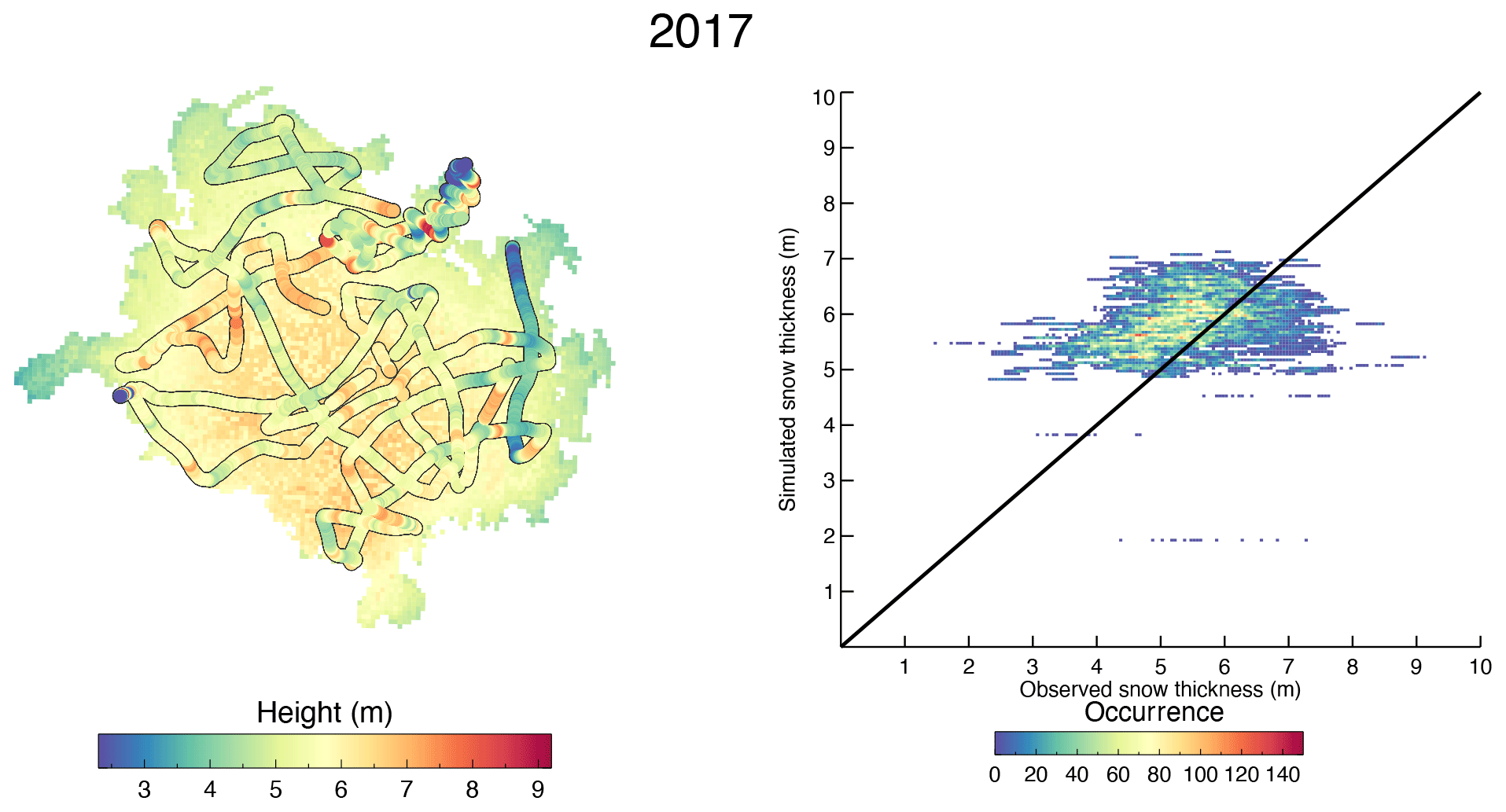
Figure 13Simulated and GPR observed snow depth for 2017 but with no effect of sublimation from snow drift in the simulations.
5.3 Albedo
As discussed earlier, Crocus calculates albedo based upon the modeled snow properties, while Noah-MP albedo is dependent on snow age alone. To compare modeled versus observed albedo, we use observations from MODIS Terra and MODIS Aqua daily snow cover and albedo products. To investigate different regions of the glacier (accumulation versus ablation area), we picked two different locations of the glacier. Figure 14 shows the albedo near the top of the glacier, where the accumulated snow typically does not melt to bare ice during summer (see Fig. 1 for the location). The gray dots represent albedo from MODIS Terra, and the black dots represent MODIS Aqua albedo. The solid line is albedo from Crocus, while the dashed line is albedo from Noah-MP. The albedo is shown for the months May through August for each modeled year; thus, the start of the melting season is included. Figure 15 shows the same as Fig. 14 but is closer to the north–northwest edge of the glacier (see Fig. 1 for the location), where accumulated snow often completely melts during the summer season. As can be seen, the modeled albedo at both locations lines up well with the observed albedo. The decrease in albedo at the end of the accumulation season, as the snow is aging, is well captured for both Noah-MP and Crocus. This is especially evident in 2015 in Fig. 15.
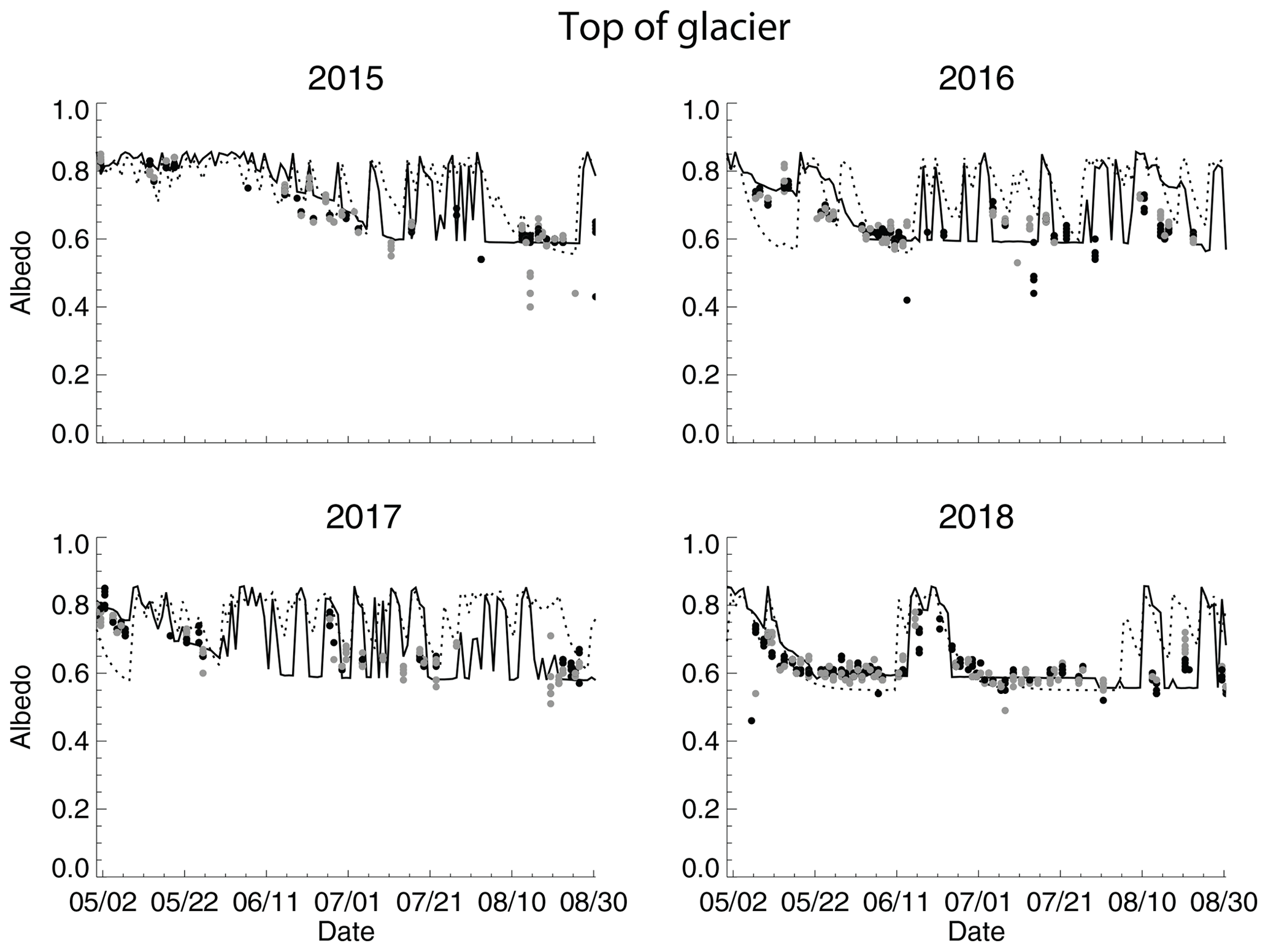
Figure 14Observed and modeled albedo at the top of Hardangerjøkulen. Dots represent observed albedo from the MODIS satellite (gray – Terra; black – Aqua). The solid line is albedo from the Crocus snow model, and the dashed line is albedo from the Noah-MP snow model.
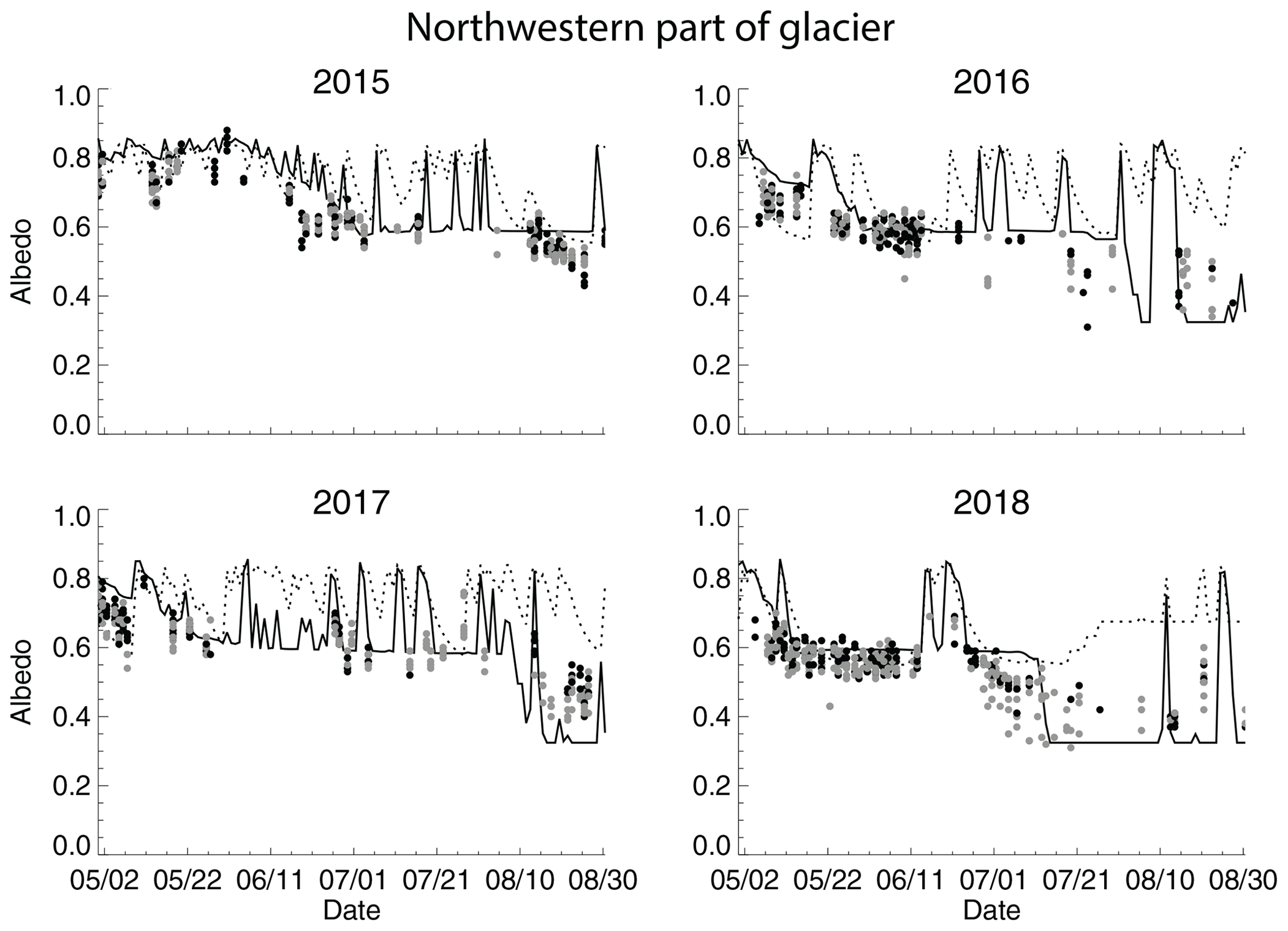
Figure 15Same as Fig. 14 but at a northwestern part of Hardangerjøkulen, where snow completely melts to the ice surface at times.
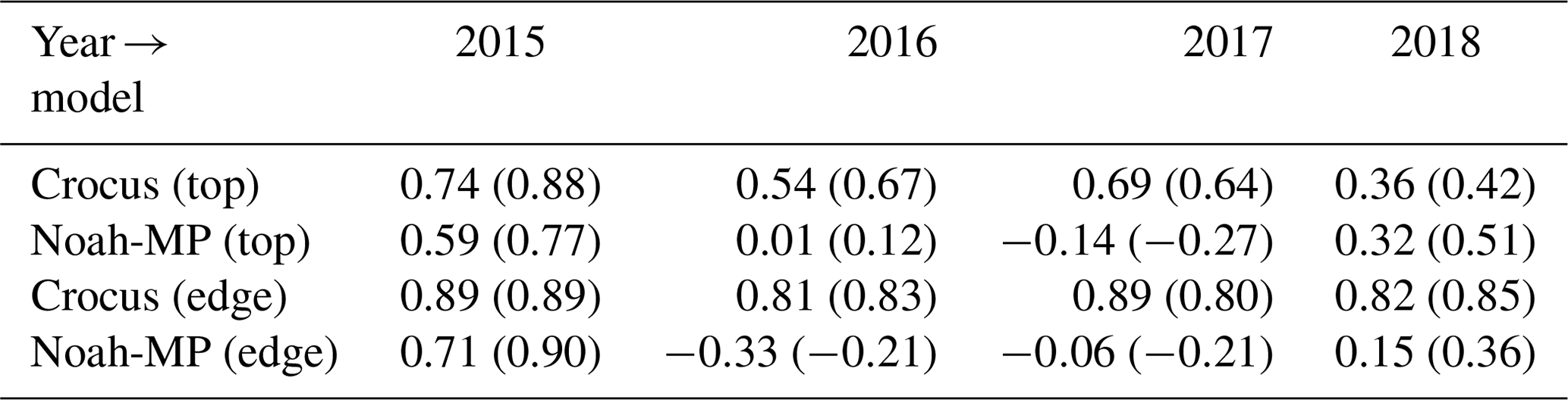
The rapid increase in albedo throughout the summer is due to snow events. The albedo determined with Crocus typically decreases rapidly after an event, since the albedo is based upon snow properties, the change in the snow properties over time and the thickness of the snow layer. Noah-MP albedo, on the other hand, decreases slower after each snow event, since it is only dependent on the snow age. At the edge of the glacier (Fig. 15), the observations show a gradual decrease in albedo as the snow starts to melt away to the bare ice (see, for example, July in 2016 and 2018 in Fig. 15), while the Crocus model has a more abrupt decrease as the snow is completely melted away. The lowest value of albedo in Crocus over the ice is 0.35. The Noah-MP does not have this decrease in albedo as the land surface category over glacier grid points is assumed to be that of old snow with a minimum albedo of 0.675. Therefore, since snow in the three-layer snow model is allowed to have lower albedo than 0.675 when the bare land surface category (glacier) is revealed, the albedo actually increases (see 2018 in Fig. 15). The correlation coefficients between modeled and observed albedo are given in Table 2. Overall, the Crocus albedo compares much better with the observations than the Noah-MP albedo in the summertime when the snow melts and the ice becomes apparent due to the assumption of glacier land surface category in Noah-MP.
Table 2Correlation coefficient between simulated and observed albedo. Values not in parenthesis are albedo from Modis Aqua, while values in parenthesis are albedo from Modis Terra.
5.4 Discharge
Figure 2 includes the catchment areas of the Middalselvi (which is fed by Midtdalsbreen) and Finseelvi locations where discharge measurements were gathered in 2017 and 2018. Figure 16 shows the modeled and observed discharge in Middalselvi for summer 2017 and 2018. Also shown is the daily precipitation at Finse station. The modeled precipitation at the Finse AWS station compares well with the observed, except for one precipitation event in late July 2017, where the model predicts too much precipitation at the Finse station. During the precipitation events, both the Crocus and Noah-MP simulations and observations show increases in discharge but with some variability in strength. Interestingly, during the large dry events at the end of June and through most of July of 2018, the modeled and observed discharge is very similar.
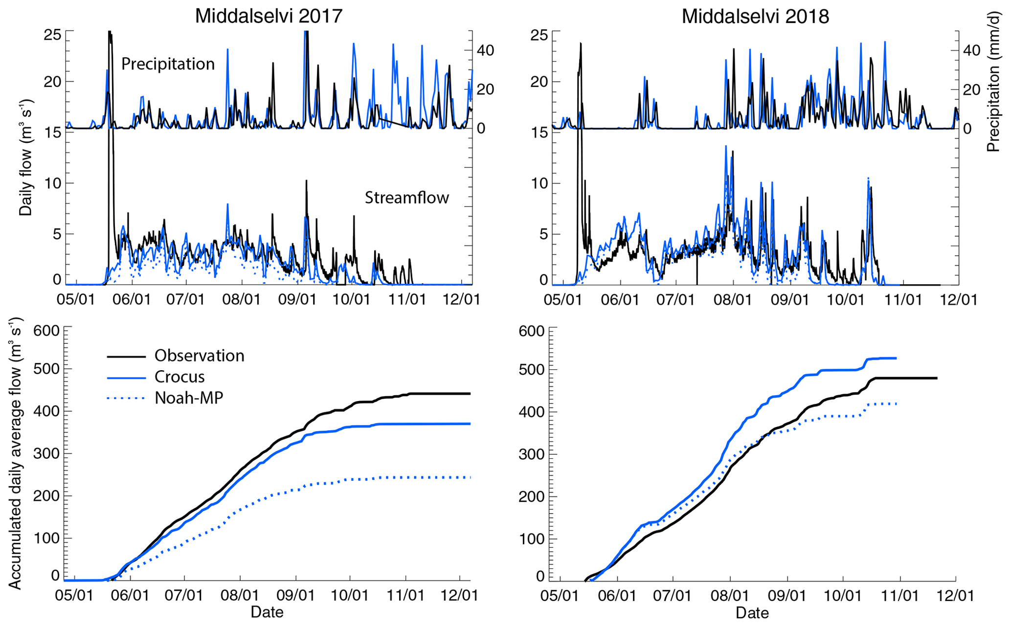
Figure 16The top panels show the observed (black line) and modeled (blue) precipitation at the Finse AWS station and daily discharge at Middalselvi. The bottom panels show the accumulated discharge. The solid blue line refers to Crocus, and the dashed blue line refers to Noah-MP.
With regards to the observed peak flow at the beginning of the melt season in May, the model does not predict such a peak flow. These peaks mark the onset of the hydrologic season in the rivers. They occurred almost at the same time in the two catchments in 2 consecutive years under similar preconditions. Photographs taken on site prior to the event indicate that water was flowing over the snowpack and was carving down to the river bed during the event. Probably some part of the peak is due to a pulsed meltwater flux and/or the associated pressure buildup to that time, which is subsequently released. Therefore, when evaluating the accumulated discharge, we start the accumulated period directly after the large spike in the observations. The accumulated discharge for 2017 shows that the observations are slightly higher than the discharge simulated with WRF-Hydro/Glacier (with Crocus). They still follow closely, but WRF-Hydro/Glacier flattens out in the fall, earlier when compared to observations. This is likely due to lack of using the baseflow or groundwater module in these specific WRF-Hydro/Glacier simulations, which could add some water to the surface streamflow. The WRF-Hydro simulations with only Noah-MP are consistently much lower compared to both observations and WRF-Hydro/Glacier at Middalselvi. For 2018, simulations with both Noah-MP over the glacier and Crocus over the glacier follow the observations reasonably well; however, they both overpredict the discharge at the end of May and early June. Around 30 July, the Crocus simulations increase slightly more than the observations, while the Noah-MP simulations reduce discharge considerably at the end of August. The Crocus simulations still have discharge comparable with the observations until September. As shown in Fig. 8j, Crocus has a larger negative summer mass balance compared to the observations, which the large discharge in early June in both Noah-MP and Crocus is likely connected to. Thus, even though Noah-MP compares well with observations at the end of the melt season in 2018, this is most likely due to too much melt in the beginning of the melt season and not the skill of the Noah-MP simulations.
One of the reasons for the lower discharge in Middalselvi with the Noah-MP compared to Crocus is likely the lack of glacier runoff once the seasonal snowpack has melted. The Middalselvi is about 60 % glacierized, while Finseelvi is only 14.7 % glacierized. As can be seen in the discharge data for Finseelvi (Fig. 17), the Noah-MP compares better with the observations in the entire melt season than it does for Middalselvi (especially in 2017; in 2018, the discharge is too high at end of May and beginning of June, as discussed above). Crocus is not shown in Fig. 17 since, in this specific setup, the Crocus simulation only feeds rivers downstream of Hardangerjøkulen, and the WRF-Hydro/Glacier system uses the Noah-MP snow model in the Finseelvi catchment area.
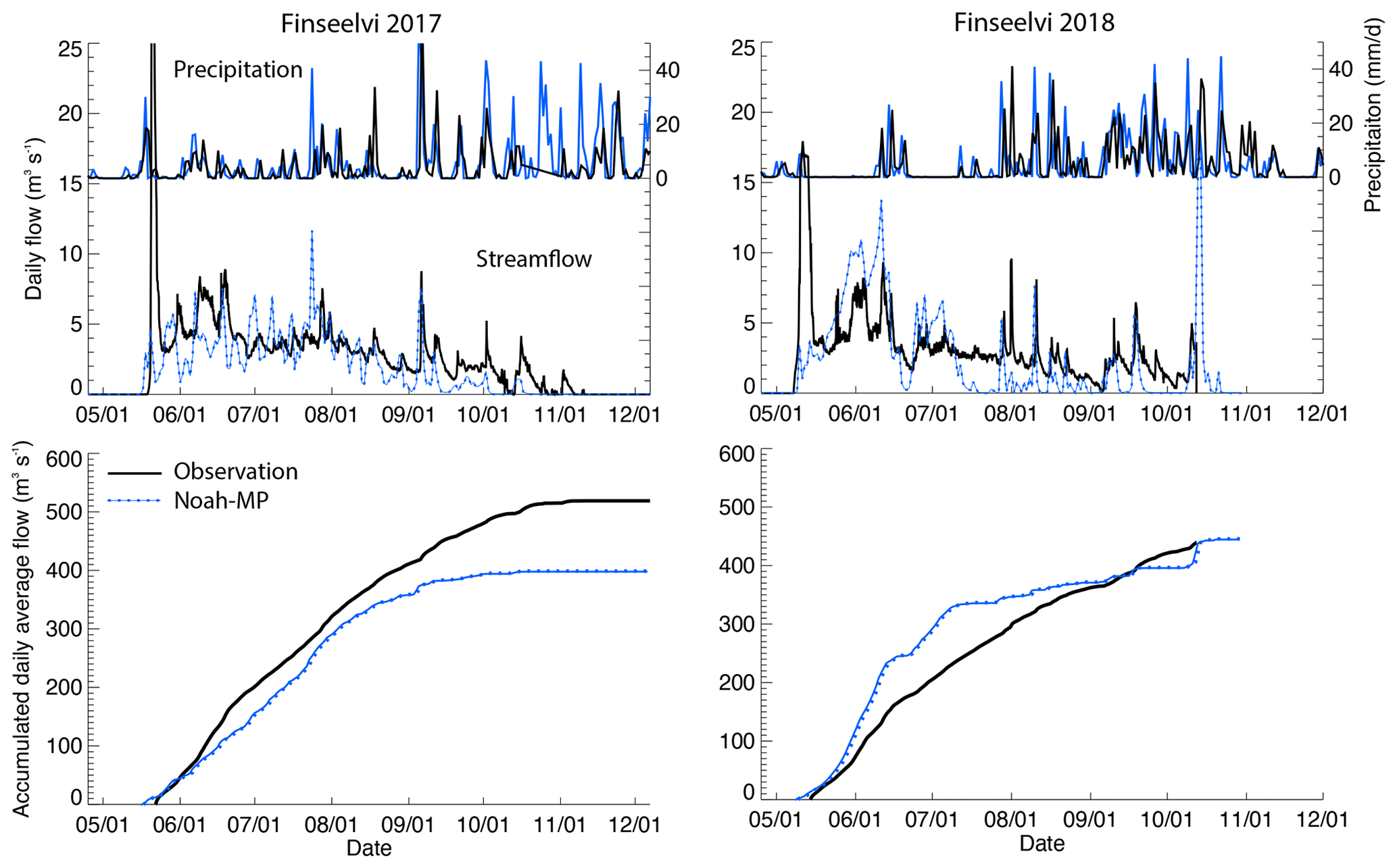
Figure 17Same as Fig. 16 but for Finseelvi. Note that, in this watershed, the WRF-Hydro/Glacier system is not using Crocus but Noah-MP due to the lack of glaciers.
We hypothesize that a second reason for the lower discharge with Noah-MP compared to Crocus is likely the albedo treatment. In 2017, there are many small snow accumulation events. This causes the Noah-MP albedo to rarely go below 0.7 at the top of the glacier (Fig. 14). However, both observations and Crocus simulations have albedo closer to 0.6. At the edge of the glacier (Fig. 15), the times where Crocus is close to 0.6 is longer, and in August, the albedo for both Crocus and the observations are around or below 0.4. For 2018, the albedo of both Noah-MP and Crocus compares well with the observations at the top of the glacier, due to the prolonged dry periods (no new snow events that lead to overestimation of albedo in Noah-MP). During this dry time period, the discharge from Noah-MP and Crocus are comparable. At the edge of the glacier, Noah-MP overestimates the albedo from the end of July. This is when all accumulated snow is melted, and the surface is bare ice. The Noah-MP albedo increases to 0.67 (that of old snow), while Crocus and observations indicate that the albedo should be that of ice. This is also the time period where streamflow from Noah-MP significantly diverges from Crocus (Fig. 16; early July). As an illustration, we re-ran Crocus for the 2018 season and substituted ice albedo with snow albedo. Figure 18 shows the accumulated streamflow with the sensitivity study (red curve). It is clear that the streamflow is reduced compared to the original simulation from the end of July at the time period where surface albedo at the edge of the glacier is reduced to that of ice. Bonekamp et al. (2019) found that the recharge of snow albedo from summer snow events in their simulations (WRF with Noah-MP) over glaciers in the Shimshal catchment in Karakorum had a large impact on the summer mass balance. We remind the reader that, even though the final accumulated streamflow using snow albedo instead of ice albedo seems to be more in line with observations, this assumption does not actually improve the simulation as it reduces the streamflow for the wrong reason.
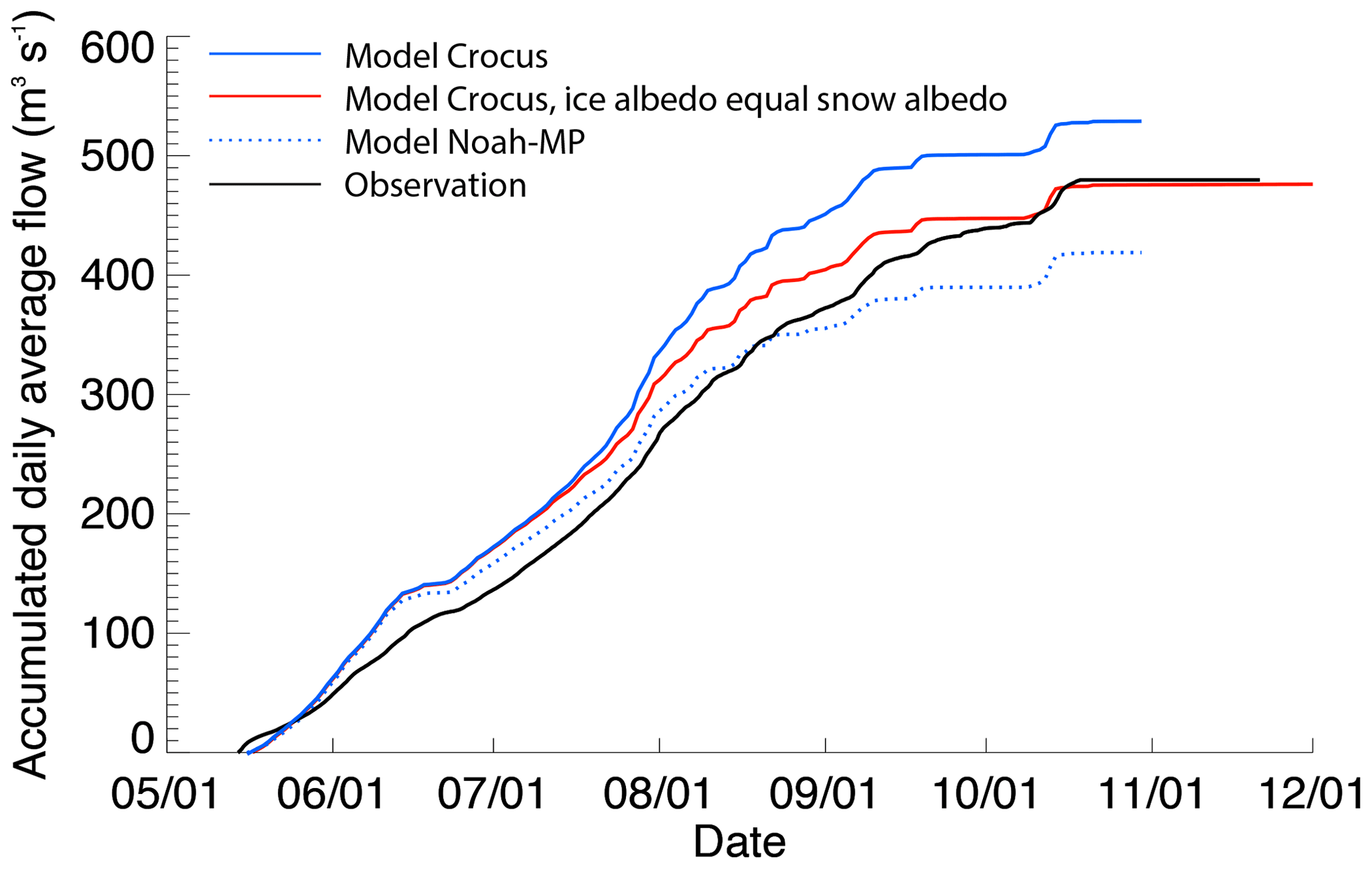
Figure 18Accumulated stream flow at Middalselvi in 2018. Red is the sensitivity test where snow albedo is used instead of ice albedo.
The detailed, physically based snow model Crocus was implemented into the WRF-Hydro system to act as a glacier model. This model supports a large number of snow layers with dynamic density, thickness and snow properties. Furthermore, the albedo is prognostically calculated based on the physical properties of the snow. The implementation of Crocus allows for a direct estimation of glacier surface winter, summer and net balance. The snow accumulation is already represented reasonably well within the WRF model when using the Noah-MP land surface model. However, the results of comparative studies performed here show that the Crocus snow model improves the simulation of melting ice by allowing for snow to melt to bare ice, using the albedo of ice for further melting instead of an assumed albedo over the glacier land surface category. This is critical for a representation of glacier wastage during the summer season. Furthermore, the integration of Crocus with WRF-Hydro allows for the discharge to be directly affected by the melting ice. Major conclusions of the evaluation of implementation of the WRF-Hydro/Glacier system and the input forcing are summarized as follows:
-
WRF produces meteorological forcing data comparable with the observations. For example, the temperature and wind speed at Finse are in excellent agreement. The 1 km grid spacing simulation results are used for input to the WRF-Hydro/Glacier system to evaluate glacier surface mass balance and subsequent streamflow.
-
Observed solid precipitation on Finse is affected by undercatch due to strong winds. Using observed precipitation from this location without correcting for this undercatch will result in an underestimation of winter surface mass balance. However, the high-resolution model simulations with WRF at 1 km show a great ability to produce winter precipitation. This can also be seen in the generally good agreement of the winter mass balance.
-
The simulations with Crocus are doing a reasonable job in reproducing winter, summer and annual surface mass balance with bias of less than 11 % in summer and about 15 % in winter (excluding 2017, which have a bias in forcing data). Noah-MP is doing slightly better than Crocus in simulating winter mass balance but cannot be used to directly evaluate the summer mass balance since Noah-MP can only melt accumulated snow from simulation start, and there is a lack of preexisting ice in the initialization of the simulation.
-
Snow depth is reproduced well, compared with both the GPR observations and observations from NVE (except for 2017 compared with the NVE observations). However, the mean snow density with Crocus and Noah-MP is underestimated by 5 %–20 % compared to NVE observations, suggesting that some of the inconsistency of snow depth (little bias) and mass balance (some bias) comparison is due to the bias in modeled snow density. Also note that the snow density is only measured at one location and assumed to be the same over the entire glacier. Furthermore, some of the bias between observations and model results are also likely due to not accounting for lateral snow distribution in the model.
-
By applying Crocus over a glacier, the surface albedo is better represented in the ablation region where ice (with lower albedo compared to snow albedo) becomes present. This allows for better representation of melting and subsequent discharge in a glacier-dominated catchment with WRF-Hydro/Glacier.
In conclusion, both the more physically based snow model Crocus and Noah-MP are simulating the winter mass balance and snow thickness well. The WRF-Hydro discharge simulations in the minimally glacierized, lower-elevation catchment (Finseelvi) are also reasonable with the Noah-MP model (keeping in mind that neither WRF-Hydro nor WRF-Hydro/Glacier has been calibrated for the simulated region). Despite this, WRF-Hydro/Glacier shows a more realistic performance in the glacierized catchment due to the fact that it allows modeling of negative net mass balance and uses ice surface albedo where all accumulated snow is melted, both of which are elements that Noah-MP currently does not include. We note that we have not currently included lateral movements of the glacier or any treatment of blowing snow in WRF-Hydro/Glacier. The impacts of including these additional physical processes may afford additional improvements in annual snowpack and snowmelt representation, particularly with respect to their spatial distribution. Finally, the forcing at 1 km does not account for any topographic variations in the 100 m domain; thus, snowpack evolution at 100 m scale is not included. More development and testing of WRF-Hydro/Glacier are certainly required and are currently underway. In particular, the system should be applied and assessed over other glaciated regions of the world. It is a tool that can contribute to a better understanding of future hydroclimate, especially in light of the continued widespread glacier retreat and decline in mass balance, which has profound implications for future water resources in many parts of the world.
The code for WRF-Hydro/Glacier used in this paper can be found at https://staff.ral.ucar.edu/trude/EVOGLAC/NDHMS_glac_fields.tar in the NDHMS_glac_fields.tar file (Eidhammer, 2021a).
Data to produce the figures can be found at https://staff.ral.ucar.edu/trude/EVOGLAC (Eidhammer, 2021b) in the outputfiles_for_figures.tar file.
TE was responsible for coupling the Crocus model to the WRF-Hydro system, running the simulations, analyzing the results, writing the paper, producing figures and acquiring the funding. AB was responsible for the GPR observations and data quality control. SD was responsible for the streamflow observations and data quality control. LL was responsible for the management of the EvoGlac research project, preparing WRF-Hydro input files, producing figures and acquiring the funding. MB was responsible for the expert input of the Noah-MP land surface model. DG was responsible for the conceptualization, funding acquisition, expert input on WRF-Hydro and scientific input. RR was responsible for the conceptualization, funding acquisition and scientific input. KM was responsible for providing glacier data. AN was responsible for the conceptualization, funding acquisition and scientific input and was the overall principal investigator. of the EvoGlac project. SS was responsible for the conceptualization, funding acquisition and scientific input.
The authors declare that they have no conflict of interests.
The hydrologic fieldwork is funded by the Strategic Research Initiative of Land Atmosphere Interaction in Cold Environments (LATICE) at the University of Oslo. Radar fieldwork was partly funded by the European Union's Horizon 2020 INTERACT project (grant no. 730938), Snow Accumulation Patterns on Hardangerjøkulen Ice Cap (SNAP), NERC SPHERES DTP (grant no. NE/L00257) and NERC Industrial CASE Studentship (grant no. NE/P009492/1). Field surveys were supported by Emma Pearce and Siobhan Killingbeck (University of Leeds) and the logistics expertise of Kjell Magne Tangen (Tajo AS). Jostein Bakke (University of Bergen – UiB) supplied the GPR system for the 2017 survey. Atle Nesje received funding from Department of Earth Science at UiB. Kjetil Melvold received funding from NVE. The National Center for Atmospheric Research is sponsored by the US National Science Foundation (NSF). We would like to acknowledge high-performance computing support from Cheyenne (https://doi.org/10.5065/D6RX99HX) provided by NCAR's Computational and Information Systems Laboratory and sponsored by the NSF. Hallgeir Elvehøy (NVE) is acknowledged, for his valuable help and comments on the glacier mass balance data.
This research has been supported by the Research Council of Norway (grant no. 255049).
This paper was edited by Jim Freer and reviewed by Emily Collier and one anonymous referee.
Aas, K. S., Dunse, T., Collier, E., Schuler, T. V., Berntsen, T. K., Kohler, J., and Luks, B.: The climatic mass balance of Svalbard glaciers: a 10-year simulation with a coupled atmosphere–glacier mass balance model, The Cryosphere, 10, 1089–1104, https://doi.org/10.5194/tc-10-1089-2016, 2016.
Andreassen, L., Elvehøy, H., Kjøllmoen, B., and Belart, J.: Glacier change in Norway since the 1960s – an overview of mass balance, area, length and surface elevation changes, J. Glaciol., 66, 313–328, https://doi.org/10.1017/jog.2020.10, 2020.
Andreassen, L. M. and Winsvold, S. H. (Eds.): Inventory of Norwegian glaciers, NVE Report 38, NVE – Norwegian Water Resources and Energy Directorate, 236 pp., 2012.
Arnault, J., Rummler, T., Baur, F., Lerch, S., Wagner, S., Fersch, B., Zhang, Z., Kerandi, N., Keil, C., and Kunstmann, H.: Precipitation sensitivity to the Uncertainty of Terrestrial Water Flow in WRF-Hydro: An Ensemble Analysis for Central Europe, J. Hydrometeorol., 19, 1007–1025, https://doi.org/10.1175/jhm-d-17-0042.1, 2018.
Ayala, A., Pellicciotti, F., and Shea, J. M.: Modeling 2 m air temperatures over mountain glaciers: Exploring the influence of katabatic cooling and external warming, J. Geophys. Res.-Atmos., 120, 3139–3157, https://doi.org/10.1002/2015JD023137, 2015.
Bolch, T., Kulkarni, A., Käaäb, A., Huggel, C., Paul, F., Cogley, J. G., Frey, H., Kargel, J. S., Fujita, K., Scheel, M., Bajracharya, S., and Stoffel, M.: The state and fate of Himalayan glaciers, Science, 336, 310–314, https://doi.org/10.1126/science.1215828, 2012.
Bonekamp, P. N. J., de Kok, R. J., Collier, E., and Immerzeel, W. W.: Contrasting meteorological drivers of the glacier mass balance between the Karakoram and central Himalaya, Front. Earth Sci., 7, 107, https://doi.org/10.3389/feart.2019.00107, 2019.
Booth, A. D., Clark, R. A., and Murray, T.: Influences on the resolution of GPR velocity analyses and a Monte Carlo simulation for establishing velocity precision, Near Surf. Geophys., 9, 399–411, https://doi.org/10.3189/2013AoG64A044, 2011.
Booth, A. D., Mercer, A., Clark, R. A., Murray, T., Jansson, P., and Axtell, C.: A comparison of seismic and radar methods to establish the thickness and density of snow cover, Ann. Glaciol., 54, 73–82, https://doi.org/10.3997/1873-0604.2011019, 2013.
Brun, E., Martin, E., Simon, V., Gendre, C., and Coléou, C.: An energy and mass model of snow cover suitable for operational avalanche forecasting, J. Glaciol., 35, 333–342, https://doi.org/10.3189/S0022143000009254, 1989.
Brun, E., David, P., Sudul, M., and Brunot, G.: A numerical model to simulate snow-cover stratigraphy for operational avalanche forecasting, J. Glaciol., 38, 13–22, https://doi.org/10.3189/S0022143000009552, 1992.
Brun, E., Martin, E., and Spiridonov, V.: Coupling a multi-layered snow model with a GCM, Ann. Glaciol., 25, 66–72, https://doi.org/10.3189/S0260305500013811, 1997.
Collier, E., Mölg, T., Maussion, F., Scherer, D., Mayer, C., and Bush, A. B. G.: High-resolution interactive modelling of the mountain glacier–atmosphere interface: an application over the Karakoram, The Cryosphere, 7, 779–795, https://doi.org/10.5194/tc-7-779-2013, 2013.
Collier, E., Maussion, F., Nicholson, L. I., Mölg, T., Immerzeel, W. W., and Bush, A. B. G.: Impact of debris cover on glacier ablation and atmosphere–glacier feedbacks in the Karakoram, The Cryosphere, 9, 1617–1632, https://doi.org/10.5194/tc-9-1617-2015, 2015.
Eidhammer, T.: WRF-Hydro/Glacier Model, https://staff.ral.ucar.edu/trude/EVOGLAC/NDHMS_glac_fields.tar, last access: 7 July 2021.
Eidhammer, T.: Model Results https://staff.ral.ucar.edu/trude/EVOGLAC, last access: 7 July 2021b.
Engelhardt, M., Schuler, T. V., and Andreassen, L. M.: Evaluation of gridded precipitation for Norway using glacier mass-balance measurements, Geograf. Ann. A, 94, 501–509, https://doi.org/10.1111/j.1468-0459.2012.00473.x, 2012.
Fersch, B., Senatore, A., Adler, B., Arnault, J., Mauder, M., Schneider, K., Völksch, I., and Kunstmann, H.: High-resolution fully coupled atmospheric–hydrological modeling: a cross-compartment regional water and energy cycle evaluation, Hydrol. Earth Syst. Sci., 24, 2457–2481, https://doi.org/10.5194/hess-24-2457-2020, 2020.
Gerbaux, M., Genthon, C., Etchevers, P., Vincent, C., and Dedieu, J.: Surface mass balance of glacier in the French Alps: Distributed modeling sensitivity to climate change, J. Glaciol., 175, 561–572, https://doi.org/10.3189/172756505781829133, 2005.
Gochis, D. J., Yu, W., and Yates, D. N.: The WRF-Hydro Model Technical Description and User's Guide, Version 3.0, NCAR Technical Document, WRF-Hydro 30 User Guide, p. 120, available at: https://ral.ucar.edu/projects/wrf_hydro/technical-description-user-guide (last access: 14 June 2021), 2015.
Hall, D. K. and Riggs, G. A.: MODIS/Aqua Snow Cover Daily L3 Global 0.05 Deg CMG, Version 6, NASA National Snow and Ice Data Center Distributed Active Archive Center, Boulder, Colorado, USA, https://doi.org/10.5067/MODIS/MYD10C1.006, 2016.
Hines, K. M., Bromwich, D. H., Bai, L.-S., Barlage, M., and Slater, A. G.: Development and testing of Polar WRF. Part III: Arctic land, J. Climate, 24, 26–48, https://doi.org/10.1175/2010JCLI3460.1, 2011.
Hong, S.-Y., Noh, Y., and Dudhia, J.: A new vertical diffusion package with an explicit treatment of entrainment processes, Mon. Weather Rev., 134, 2318–2341, https://doi.org/10.1175/MWR3199.1, 2006.
Iacono, M. J., Jennifer, S. D., Eli, J. M., Mark, W. S., Shepard, A. C., and William, D. C.: Radiative forcing by long-lived greenhouse gases: calculations with the AER radiative transfer models, J. Geophys. Res.-Atmos., 113, D13103, https://doi.org/10.1029/2008JD009944, 2008.
Immerzeel, W., Pellicciotti, F., and Bierkens, M.: Rising river flows throughout the twenty-first century in two Himalayan glacierized watersheds, Nat. Geosci., 6, 742–745, https://doi.org/10.1038/ngeo1896, 2013.
Immerzeel, W. W., Beek, L. P. H. V., and Bierkens, M. F. P.: Climate change will affect the Asian water towers, Science, 328, 1382–1385, https://doi.org/10.1126/science.1183188, 2010.
Jarosch, A. H., Anslow, F. S., and Clarke, G. K.: High-resolution precipitation and temperature downscaling for glacier models, Clim. Dynam., 38, 391–409, 2012
Jordan, R.: A one-dimensional temperature model for a snow cover, Spec. Rep. 91-16, Cold Reg. Res. and Eng. Lab., US Army Corps of Eng., Hanover, NH, 1991.
Kaser, G., Großhauser, M., and Marzeion, B.: Contribution potential of glaciers to water availability in different climate regimes, P. Natl. Acad. Sci. USA, 107, 20223–20227, https://doi.org/10.1073/pnas.1008162107, 2010.
Kjøllmoen, B. (Ed.), Andreassen, L. M., Elvehøy, H., Jackson, M., Kjøllmoen, B., and Giesen, R. H.: Glaciological investigations in Norway 2011–2015, NVE Report 88/2016, NCR, Oslo, Norway, 171 pp., 2016
Kjøllmoen, B. (Ed.), Andreassen, L. M., Elvehøy, H., Jackson, M., Melvold, K., and Kjøllmoen, B.: Glaciological investigations in Norway in 2016, NVE Report 76/2017,NCR, Oslo, Norway, 95 pp., 2017.
Kjøllmoen, B. (Ed.), Andreassen, L. M., Elvehøy, H., and Jackson, M.: Glaciological investigations in Norway in 2017, NVE Report 82/2018, NCR, Oslo, Norway, 84 pp., 2018.
Kjøllmoen, B. (Ed.), Andreassen, L. M., Elvehøy, H., and Jackson, M.: Glaciological investigations in Norway in 2018, NVE Report 46/2019, NCR, Oslo, Norway,, 84 pp., 2019.
Kotlarski, S., Paul, F., and Jacob, D.: Forcing a distributed glacier mass balance model with the regional climate model REMO. Part I: climate model evaluation, J. Climate, 23, 1589–1606, https://doi.org/10.1175/2009JCLI2711.1, 2010a.
Kotlarski, S., Jacob, D., Podzun, R., and Paul, F.: Representing glaciers in a regional climate model, Clim. Dynam., 34, 27–46, https://doi.org/10.1007/s00382-009-0685-6, 2010b.
Laghari, J.: Climate change: Melting glaciers bring energy uncertainty, Nature, 502, 617–618, https://doi.org/10.1038/502617a, 2013.
Li, L., Gochis, D. J., Sobolowski, S., and Mesquita, M. D. S.: Evaluating the present annual water budget of a Himalayan headwater river basin using a high-resolution atmosphere-hydrology model, J. Geophys. Res., 122, 4786–4807, https://doi.org/10.1002/2016JD026279, 2017.
Liston, G. and Sturm, M.: A snow-transport model for complex terrain, J. Glaciol., 44, 498–516, https://doi.org/10.3189/S0022143000002021, 1998.
Liu, C., Ikeda, K., Rasmussen, R., Barlage, M., Newman, A. J., Prein, A. F., Chen, F., Chen, L., Clark, M., Dai, A., Dudhia, J., Eidhammer, T., Gochis, D., Gutmann, E., Kurkute, S., Li, Y., Thompson, G., and Yates, D.: Continental-scale convection-permitting modeling of the current and future climate of North America, Clim. Dynam., 49, 71–95, https://doi.org/10.1007/s00382-016-3327-9, 2017.
Lundquist, J., Hughes, M., Gutmann, E., and Kapnick, S.: Our skill in modeling mountain rain and snow is bypassing the skill of our observational networks, B. Am. Meteorol. Soc., 100, 2473–2490, https://doi.org/10.1175/BAMS-D-19-0001.1, 2019.
Machguth, H., Paul, F., Kotlarski, S., and Hoelzle, M.: Calculating distributed glacier mass balance for the Swiss Alps from regional climate model output: a methodical description and interpretation of the results, J. Geophys. Res.-Atmos., 114, 1–19, https://doi.org/10.1029/2009JD011775, 2009.
Melvold, K., Laumann, T., and Nesje, A.: Kupert landskap under Hardangerjøkulen [Online], GEO, Norge, available at: http://www.geoforskning.no/reportasjene/38-kupert-landskap-under-hardangerjokulen (last access: 14 June 2021), 2011.
Mölders, N. and Kramm, G.: A case study on wintertime inversions in Interior Alaska with WRF, Atmos. Res., 95, 314–332, https://doi.org/10.1016/j.atmosres.2009.06.002, 2010.
Mölg, T. and Kaser, G.: A new approach to resolving climate–cryosphere relations: downscaling climate dynamics to glacier-scale mass and energy balance without statistical scale linking, J. Geophys. Res., 116, D16101, https://doi.org/10.1029/2011JD015669, 2011.
Niu, G. Y., Yang, Z. L., Mitchell, K. E., Chen, F., Ek, M. B., Barlage, M., Kumar, A., Manning, K., Niyogi, D., Rosero, E., Tewari, M., and Xia, Y.: The community Noah land surface model with multiparameterization options (Noah-MP): 1. Model description and evaluation with local-scale measurements, J. Geophys. Res.-Atmos., 116, 1–19, https://doi.org/10.1029/2010JD015139, 2011.
Quéno, L., Vionnet, V., Dombrowski-Etchevers, I., Lafaysse, M., Dumont, M., and Karbou, F.: Snowpack modelling in the Pyrenees driven by kilometric-resolution meteorological forecasts, The Cryosphere, 10, 1571–1589, https://doi.org/10.5194/tc-10-1571-2016, 2016.
Rasmussen, R., Baker, B., Kochendorfer, J., Meyers, T., Landolt, S., Fischer, A. P., Black, J., Thriault, J. M., Kucera, P., Gochis, D., Smith, C., Nitu, R., Hall, M., Ikeda, K., and Gutmann, E.: How well are we measuring snow: the NOAA/FAA/NCAR winter precipitation test bed, B. Am. Meteorol. Soc., 93, 811–829, https://doi.org/10.1175/BAMS-D-11-00052.1, 2012.
Réveillet, M., Six, D., Vincent, C., Rabatel, A., Dumont, M., Lafaysse, M., Morin, S., Vionnet, V., and Litt, M.: Relative performance of empirical and physical models in as- sessing the seasonal and annual glacier surface mass balance of Saint-Sorlin Glacier (French Alps), The Cryosphere, 12, 1367–1386, https://doi.org/10.5194/tc-12-1367-2018, 2018.
Revuelto, J., Vionnet, V., López-Moreno, J.-I., Lafaysse, M., and Morin, S.: Combining snowpack modeling and terrestrial laser scanner observations improves the simulation of small scale snow dynamics, J. Hydrol., 533, 291–307, https://doi.org/10.1016/j.jhydrol.2015.12.015, 2016.
Rummler, T., Arnault, J., Gochis, D., and Kunstmann, H.: Role of Lateral Terrestrial Water Flow on the Regional Water Cycle in a ComplexTerrain Region: Investigation With a Fully Coupled Model System, J. Geophys. Res.-Atmos., 124, 507–529, https://doi.org/10.1029/2018jd029004, 2019.
Senatore, A., Mendicino, G., Gochis, D. J., Yu, W., Yates, D. N., and Kunstmann, H.: Fully coupled atmosphere-hydrology simulations for the central Mediterranean: Impact of enhanced hydrological parameterization for short and long time scales, J. Adv. Model. Earth Syst., 7, 1693–1715, https://doi.org/10.1002/2015MS000510, 2015.
Skamarock, W. C., Klemp, J. B., Dudhi, J., Gill, D. O., Barker, D. M., Duda, M. G., Huang, X.-Y., Wang, W., and Powers, J. G.: A Description of the Advanced Research WRF Version 3, Technical Report 113, Tech. Note, Mesoscale and Microscale Meteorology Division, NCAR – National Center for Atmospheric Research, Boulder, Colorado, USA, 2008.
Smith, C. D., Ross, A., Kochendorfer, J., Earle, M. E., Wolff, M., Buisán, S., Roulet, Y., and Laine, T.: The Post-SPICE (2015/2016 and 2016/2017) Winter Precipitation Intercomparison Data, PANGAEA, https://doi.org/10.1594/PANGAEA.907379, 2019.
Smith, C. D., Ross, A., Kochendorfer, J., Earle, M. E., Wolff, M., Buisán, S., Roulet, Y.-A., and Laine, T.: Evaluation of the WMO Solid Precipitation Intercomparison Experiment (SPICE) transfer functions for adjusting the wind bias in solid precipitation measurements, Hydrol. Earth Syst. Sci., 24, 4025–4043, https://doi.org/10.5194/hess-24-4025-2020, 2020.
Smith, R. B. and Barstad, I.: A Linear Theory of Orographic Precipitation, J. Atmos. Sci., 61, 1377–1391, 2004.
Sorg, A., Bolch, T., Stoffel, M., Solomina, O., and Beniston, M.: Climate change impacts on glaciers and runoff in Tien Shan (Central Asia), Nat. Clim. Change, 2, 725–731, https://doi.org/10.1038/nclimate1592, 2012.
Thompson, G. and Eidhammer, T.: A study of aerosol impacts on clouds and precipitation development in a large winter cyclone, J. Atmos. Sci., 71, 3636–3658, https://doi.org/10.1175/JAS-D-13-0305.1, 2014.
van Pelt, W. J. J., Oerlemans, J., Reijmer, C. H., Pohjola, V. A., Pettersson, R., and van Angelen, J. H.: Simulating melt, runoff and refreezing on Nordenskiöldbreen, Svalbard, using a coupled snow and energy balance model, The Cryosphere, 6, 641–659, https://doi.org/10.5194/tc-6-641-2012, 2012.
Vionnet, V., Brun, E., Morin, S., Boone, A., Faroux, S., Le Moigne, P., Martin, E., and Willemet, J.-M.: The detailed snowpack scheme Crocus and its implementation in SURFEX v7.2, Geosci. Model Dev., 5, 773–791, https://doi.org/10.5194/gmd-5-773-2012, 2012.
Vionnet, V., Six, D., Auger, L., Dumont, M., Lafaysse, M., Quéno, L., Réveillet, M., Dombrowski-Etchevers, I., Thibert, E., and Vincent, C.: Sub-kilometer Precipitation Datasets for Snowpack and Glacier Modeling in Alpine Terrain, Front. Earth Sci., 7, 182, https://doi.org/10.3389/feart.2019.00182, 2019.
Yucel, I., Onen, A., Yilmaz, K. K., and Gochis, D. J.: Calibration and evaluation of a flood forecasting system: Utility of numerical weather prediction model, data assimilation and satellite-based rainfall, J. Hydrol., 523, 49–66, https://doi.org/10.1016/j.jhydrol.2015.01.042, 2015.