the Creative Commons Attribution 4.0 License.
the Creative Commons Attribution 4.0 License.
 | 29 Jul 2021
Development and evaluation of 0.05° terrestrial water storage estimates using Community Atmosphere Biosphere Land Exchange (CABLE) land surface model and assimilation of GRACE data
Natthachet Tangdamrongsub
Michael F. Jasinski
Peter J. Shellito
Accurate estimation of terrestrial water storage (TWS) at a high spatiotemporal resolution is important for reliable assessments of regional water resources and climate variability. Individual components of TWS include soil moisture, snow, groundwater, and canopy storage and can be estimated from the Community Atmosphere Biosphere Land Exchange (CABLE) land surface model. The spatial resolution of CABLE is currently limited to 0.5∘ by the resolution of soil and vegetation data sets that underlie model parameterizations, posing a challenge to using CABLE for hydrological applications at a local scale. This study aims to improve the spatial detail (from 0.5 to 0.05∘) and time span (1981–2012) of CABLE TWS estimates using rederived model parameters and high-resolution meteorological forcing. In addition, TWS observations derived from the Gravity Recovery and Climate Experiment (GRACE) satellite mission are assimilated into CABLE to improve TWS accuracy. The success of the approach is demonstrated in Australia, where multiple ground observation networks are available for validation. The evaluation process is conducted using four different case studies that employ different model spatial resolutions and include or omit GRACE data assimilation (DA). We find that the CABLE 0.05∘ developed here improves TWS estimates in terms of accuracy, spatial resolution, and long-term water resource assessment reliability. The inclusion of GRACE DA increases the accuracy of groundwater storage (GWS) estimates and has little impact on surface soil moisture or evapotranspiration. Using improved model parameters and improved state estimations (via GRACE DA) together is recommended to achieve the best GWS accuracy. The workflow elaborated on in this paper relies only on publicly accessible global data sets, allowing the reproduction of the 0.05∘ TWS estimates in any study region.
- Article
(12519 KB) - Full-text XML
-
Supplement
(153 KB) - BibTeX
- EndNote


Accurate knowledge of terrestrial water storage (TWS) is crucial for assessing water resource and climate variability (Delworth and Manabe, 1988; Koster and Suarez, 2001). TWS consists of soil moisture, groundwater, snow, and canopy storage. Each component plays a significant role in the global water cycle and interacts closely with the land–atmospheric water–energy exchange (Koster et al., 2006; Fischer et al., 2007; Seneviratne et al., 2010). The TWS components can be measured or estimated by various platforms (e.g., satellite measurement and model simulation). However, spatial resolutions are coarse due to the limitation of sensors and models that focus on global or continental scales (e.g., Rodell et al., 2004; Alkama et al., 2010). At a regional or local scale, the spatial resolution of the TWS estimate is vital, as most applications (e.g., risk management for drought or flood) require accurate information at the county or sub-county level (Quiring, 2009). This motivates the development of TWS estimates at higher spatiotemporal scales, corresponding particularly to an increased interest in exploiting TWS in interdisciplinary studies (e.g., IPCC, 2007; NASEM, 2018).
TWS information can be obtained or estimated from ground observation networks, satellite measurements, or model simulations. Each has different strengths and limitations. Ground observations (e.g., soil moisture probe and groundwater well) are considered the most reliable, providing measurements closest to the truth (e.g., Dorigo et al., 2013). However, ground observations have high maintenance costs and incomplete coverage. Also, point measurements only reflect information at one location and not necessarily the entire region. On the other hand, satellite platforms offer an automated measurement with improved coverage ranging from regional to global (e.g., Tapley et al., 2004; Entekhabi et al., 2010a). The challenges of using satellite measurements are the coarse spatial resolution and the sensors' technical limitations (e.g., penetration depth, cloud/vegetation obstruction, and background noise). Therefore, its usage is restricted to a large region and requires a sophisticated algorithm to retrieve TWS variables (Crow et al., 2012; Castellazzi et al., 2016; Tangdamrongsub et al., 2019). In addition, satellite measurements can be limited by a relatively short period of record (e.g., Flechtner et al., 2014; Karthikeyan et al., 2017).
TWS components can also be simulated from a land surface model (LSM). The LSM incorporates various land surface physics into complex numerical sequences to allow the simulation of TWS to be performed at any desired location and spatiotemporal scale (Pitman, 2003). The LSM can provide a complete suite of TWS components compared with the ground or satellite measurements that can only measure a single or integrated TWS component (e.g., Tapley et al., 2004; Entekhabi et al., 2010a). However, due to the limitations of input data, the spatial resolution of many LSMs is coarse (e.g., >0.25∘ (∼25 km)), which consequently restricts their application to a large region (e.g., Rodell et al., 2004; Alkama et al., 2010; Ke et al., 2012).
Efforts to improve the spatial resolution (and time span) of global TWS estimates have been made in many modeling communities (e.g., Wood et al., 2011; Bierkens et al., 2015; Bierkens, 2015). For instance, Ke et al. (2012) improved the resolution of the Community Land Model (CLM) from 0.5∘ (∼50 km) to 0.05∘ (∼5 km) using modified land surface parameters. The World-Wide Water model (W3; van Dijk et al., 2013a, b) recently allowed the global TWS variables to be estimated at 0.05∘ (∼5 km). The European Centre for Medium-Range Weather Forecasts (ECMWF) Reanalysis 5 (ERA5) offers global land surface variables at 0.1∘ (∼9 km) resolution from 1981 to present (see the data availability section). A similar effort is also seen in hydrologic model development, such as the PCRaster Global Water Balance (PCR-GLOBWB; Sutanudjaja et al., 2018), which improves the spatial resolution from 30 arcmin (∼50 m or ∼0.5∘) to 5 arcmin (∼9 km or 0.083∘) and extends the time span to more than a 50-year period. The enhancement of model spatial resolution and time span receives even more attention at the local level, where spatial detail down to a few kilometers is needed (e.g., Rasmussen et al., 2014; Singh et al., 2015; Beamer et al., 2016; Dong et al., 2020).
On top of the improved spatiotemporal resolutions, the improved accuracy of TWS estimates is also a concern in LSM developments. As in most environmental modeling systems, model outputs are associated with a high degree of uncertainty propagated from, e.g., inaccurate meteorological forcings, imperfect model physics, and ineffective parameter calibration. Data assimilation (DA; Reichle et al., 2002; Reichle, 2008) techniques can be employed to improve LSM performance. The approach sequentially updates the model's states using an optimal value computed by combining model simulations with observations. A variety of satellite observations reflecting different TWS components can be assimilated into the system (e.g., Kumar et al., 2014; Dong and Crow, 2018). TWS observations from the Gravity Recovery And Climate Experiment (GRACE) satellite mission (Tapley et al., 2004) offer integrated water column information that can be used to constrain multiple water storage components simultaneously (e.g., Zaitchik et al., 2008; Forman et al., 2012; Tangdamrongsub et al., 2015). GRACE DA has shown positive impacts on most TWS components, including groundwater (e.g., Girotto et al., 2017; Nie et al., 2019), soil moisture (Jung et al., 2019), and snow (Kumar et al., 2016).
The Community Atmosphere Biosphere Land Exchange model (CABLE; Kowalczyk et al., 2006) is an open-source global LSM developed and updated by the community. CABLE is a core LSM of the Australian Community Climate and Earth System Simulator (ACCESS; Bi et al., 2013; Kowalczyk et al., 2013) that can be used to simulate water storage and fluxes globally. The model has been regularly updated to incorporate state-of-the-art model physics (e.g., Decker, 2015; Ukkola et al., 2016; Haverd et al., 2018). Despite its success, CABLE's spatial scale is currently limited to 0.5∘ (∼50 km) due to the 0.5∘ resolution of its parameter and forcing data sets. This contrasts with other global model developments, where high-resolution versions have already been developed (e.g., van Dijk et al., 2013a, b; Sutanudjaja et al., 2018). CABLE and its inputs must be reconfigured to increase the spatial detail of TWS estimates for smaller-scale studies (e.g., 0.01–0.05∘). Our effort to increase the study's spatial resolution should narrow this development gap and has not previously been implemented.
This study aims to improve the accuracy, spatial resolution, and time span of CABLE TWS estimates. Our approach utilizes only publicly available global data sets, so resulting TWS estimates can be reproduced over any target region (see the data availability section for the data access). The spatial detail of CABLE is improved from 0.5 to 0.05∘ (∼5 km) using high-resolution forcing data (precipitation in particular) and land surface parameters derived from high-resolution maps of soil and vegetation cover. The development is demonstrated in Australia, where ground observation networks (e.g., surface soil moisture, groundwater, and evapotranspiration) are available to validate the result. The demonstrated simulation period is 1981–2012, coincident with the availability of meteorological forcing data. Recent studies have shown success in assimilating GRACE data into a coarse-scale CABLE version to improve TWS and groundwater storage (GWS) estimates in the Goulburn River catchment and in the North China Plain (Tangdamrongsub et al., 2020; Yin et al., 2020). In this study, GRACE observations (Luthcke et al., 2013) are also assimilated into CABLE 0.05∘ (and CABLE 0.5∘) to improve the accuracy of TWS components between 2003 and 2012. Assimilating the coarse GRACE observations into a much higher-resolution model is performed using the 3-dimensional ensemble Kalman smoother (EnKS 3D; Tangdamrongsub et al., 2017). This approach will reveal whether assimilating GRACE data can benefit a newly developed fine-scale CABLE configuration. Our study will perform a thorough investigation on this issue to address GRACE DA's benefit on CABLE 0.05∘.
The objectives of this paper are (1) to present the development and evaluation of retrospective 0.05∘ TWS estimates and (2) to assess the GRACE DA impact on 0.05∘ CABLE version, as well as the benefit of assimilating the coarse resolution satellite data into a fine-scale model. This paper is presented as follows. Section 2 provides the details of the study area, model configurations, and data processing. Section 3 presents the GRACE DA schematic and the statistical metric used in the evaluation. Section 4 presents the assessment and validation of the result. Finally, Sect. 5 summarizes the findings of this study and provides a possible direction for future development.
2.1 Study area
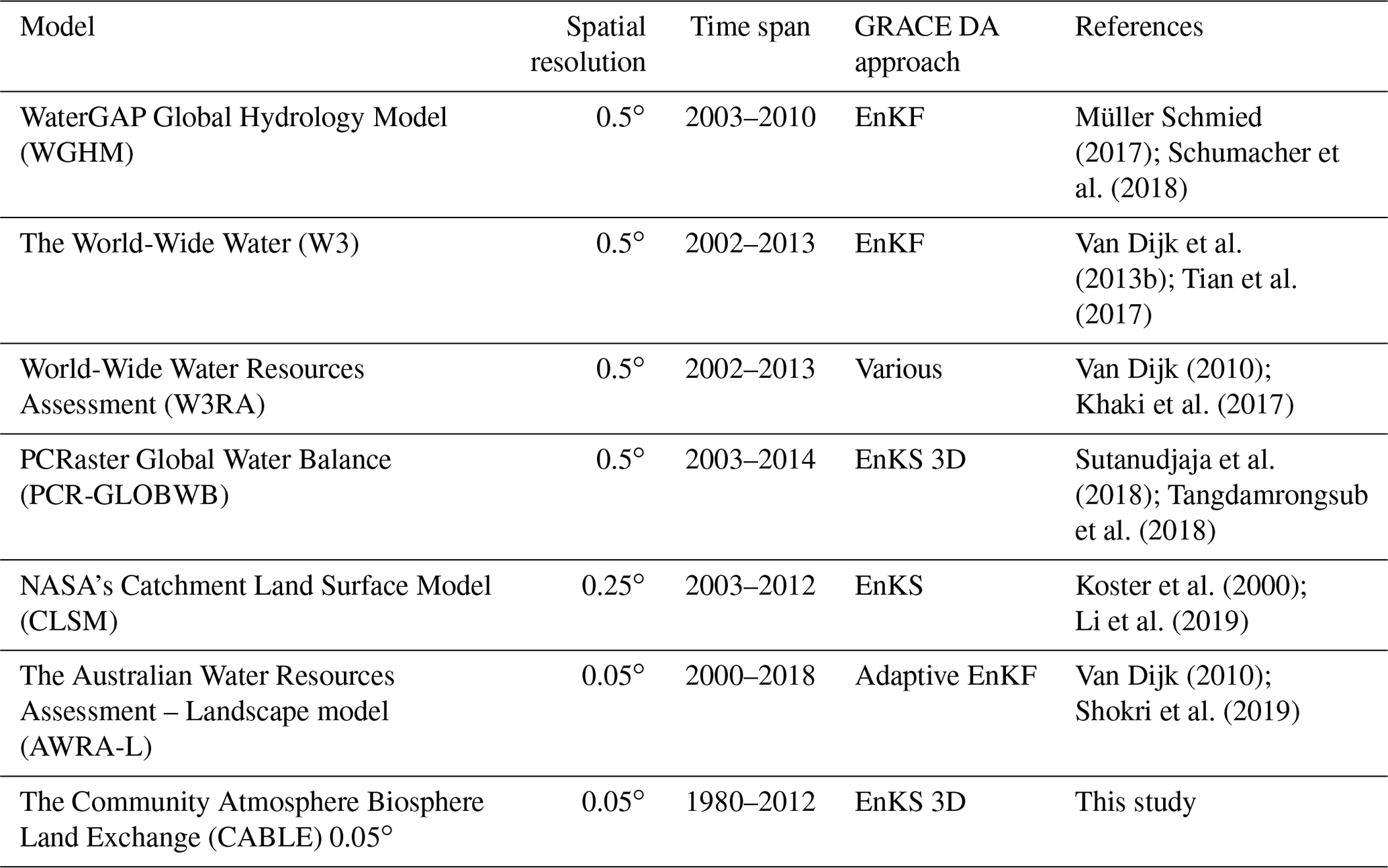
This study uses Australia as a case study. Due to its size and geographic location, Australia is influenced by multiple climate drivers (Murphy and Timbal, 2008; Xie et al., 2016) and experiences episodes of severe droughts and floods (e.g., van Dijk et al., 2013a). The recent long-term drought, known as the Millennium Drought (Bond et al., 2008), severely affected industrial and agricultural sectors and has led to a significant economic loss nationwide (see, e.g., van Dijk et al., 2013a). The need for an accurate prediction of possible water scarcity from climate variations motivated the development of land surface and hydrology models in Australia, e.g., the Australian Water Availability Project (AWAP; Raupach et al., 2008), the Australian Water Resources Assessment – Landscape Model (AWRA-L; van Dijk, 2010), and CABLE (Kowalczyk et al., 2006). Recent work has assimilated GRACE satellite data into such water models (e.g., Tian et al., 2017; Schumacher et al., 2018; Tangdamrongsub et al., 2020). Studies relevant to GRACE DA in Australia are summarized in Table 1. Ground observation networks have also been installed across the continent and continuously monitor the water storage and flux variations. Such data records are valuable for validating the accuracy of the model estimates and remote sensing observations. Details regarding the in situ data used in this study are provided in Sect. 2.3.2.
2.2 Model configuration
In this study, TWS estimates are derived from CABLE. A history of the model's development can be found in, e.g., Wang et al. (2011), Kowalczyk et al. (2013), Decker (2015), and Haverd et al. (2018). Multiple CABLE versions have been developed since 2003 for different objectives (see the data availability section); CABLE SubgridSoil GroundWater (CABLE-SSGW; Decker, 2015) is considered most suitable for our use due to its inclusion of comprehensive terrestrial water storage components and, especially, a groundwater module. CABLE is developed using Fortran and can be executed in a Unix environment. The input/output file format follows the NetCDF Climate and Forecast (CF) convention. The model has been used to simulate global TWS at 0.5∘ spatial resolution using 0.5∘ resolution model parameters and forcing data (e.g., Decker, 2015; Ukkola et al., 2016). The variables used to assess TWS consist of soil moisture storage (SMS), snow water equivalent (SWE), canopy storage (CNP), and GWS.
The model parameters of CABLE-SSGW are derived from several different sources (Kowalczyk et al., 2006; Wang et al., 2011; Decker, 2015). Land use/vegetation type categories are obtained from the International Geosphere–Biosphere Programme (IGBP) classification from the Moderate Resolution Imaging Spectroradiometer (MODIS; Friedl et al., 2002). Relative volumes of silt, sand, clay, and organic matter in the soil are obtained from the Harmonized World Soil Database (Fischer et al., 2008). The Zobler soil category (Zobler, 1999) is computed empirically from the silt, sand, and clay fractions (Oleson et al., 2010). The monthly climatology of the leaf area index (LAI) is computed using a reprocessed MODIS LAI product (Yuan et al., 2011). All derived model parameters are resampled to 0.5∘ to match the 0.5∘ model grid space. Comprehensive details of model parameters can be found in, e.g., Kowalczyk et al. (2006), Wang et al. (2011), and Decker (2015).
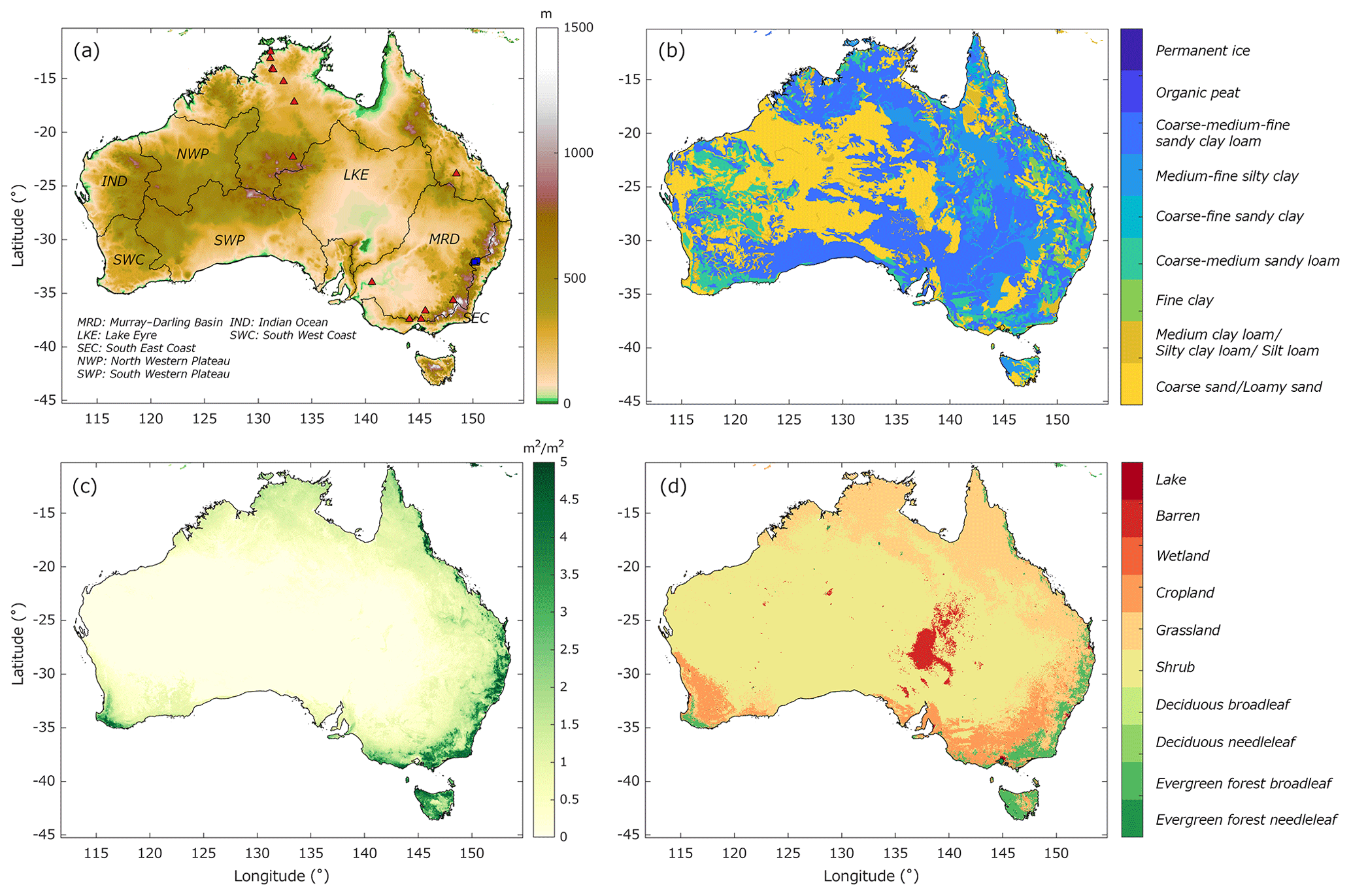
Figure 1(a) Characteristics of the study area, including elevation, major Australian river basin, and ground observation networks (FLUXNET – red triangle; the Scaling and Assimilation of Soil Moisture and Streamflow (SASMAS) – blue square). Note that the locations of groundwater sites can be found in Fig. 14. (a–c) The derived 0.05∘ land cover values for (b) soil class, (c) averaged LAI (used only for demonstration), and (d) vegetation and land cover types.
Table 1Relevant studies related to the development of the land surface and hydrology models (with the inclusion of GRACE DA applications) to estimate TWS in Australia.
This study rederives the model parameters and employs enhanced forcing data to increase the model spatial detail from 0.5 to 0.05∘. The vegetation type is derived from the global land cover climatology using MODIS data (Broxton et al., 2014). The soil map is also derived from the Harmonized World Soil Database but at 0.05∘ grid spacing. The 0.05∘ monthly climatology LAI is derived from the Global Land Surface Satellite product (GLASS; Xiao et al., 2014). All rederived parameters are shown in Fig. 1. The soil layer thicknesses, from top to bottom, are set to 1.2, 3.8, 25, 39.9, 107.9, and 287.2 cm, and the unconfined aquifer's thickness is set to 20 m. The surface soil moisture (SSM; cubic meter per cubic meter, hereafter m3 m−3) is defined as the top two layers, and the SMS (meters) is computed from all soil layers.
The CABLE model is forced with precipitation, air temperature, wind speed, humidity, surface pressure, and shortwave and longwave downward radiation. For precipitation, we use the Climate Hazards Group InfraRed Precipitation with Station data (CHIRPS; Funk et al., 2015), provided on a 0.05∘ grid. The other forcing variables are provided on a 0.5∘ grid by the high-resolution global data set of meteorological forcings for land surface modeling version 2, Princeton University (Princeton; Sheffield et al., 2006). When performing 0.5∘ model simulations, the CHIRPS data are spatially averaged to 0.5∘ grid space while other forcing variables maintain their intrinsic 0.5∘ resolution. When performing 0.05∘ model simulations, the coarser-resolution forcing variables are spatially resampled to 0.05∘ model grid space using the nearest-neighbor interpolation.
Model simulations are performed between 1981 and 2012 (a total of 32 years), given the Princeton forcing data's availability. Similar to McNally et al. (2017), temporal disaggregation is applied to CHIRP precipitation data to resample from 1 d to 3 h, consistent with the Princeton data's time step. The scale factor derived from the 3 h Princeton precipitation data is used to (temporally) rescale the CHIRPS data. The characteristics of forcing data and the derived model parameters used in this paper are given in Table 2.
Table 2Characteristics of the land cover parameters, meteorological forcing, and remote sensing data used in the development and validation of CABLE 0.05∘.

“n/a” stands for not applicable.
In all simulations, initial states are obtained using a 320-year spinup, i.e., performing 10 repeated runs between 1981 and 2012.
2.3 GRACE data
GRACE is a twin satellite-to-satellite tracking mission designed to measure the mean and time-varying components of the Earth's gravity field (Tapley et al., 2004). Every month, GRACE provides a time-varying gravity solution containing information about mass redistribution near the Earth's surface. The monthly gravity change is dominated by a hydrology signal, making the GRACE product beneficial for various hydrological and geophysical applications (e.g., Klees et al., 2008; Mouyen et al., 2018; Rodell et al., 2018; Tapley et al., 2019). Different GRACE solutions have been released, including the mascon solution (e.g., Luthcke et al., 2008; Rowlands et al., 2010). The mascon approach utilizes mass concentration blocks (as a basis function) to determine the Earth's mass variation and is found to provide a more accurate TWS estimate compared to the spherical harmonic approach (Rowlands et al., 2010). In this study, the mascon (mass concentration) product from the Goddard Space Flight Center (GSFC) is used (Luthcke et al., 2013). The GSFC Mascon product contains monthly TWS variations (ΔTWS), expressed in equivalent water height (in, e.g., meters). The glacial isostatic adjustment correction is applied using the ICE6G model (Peltier et al., 2015). The mascon varies in size and represents the average ΔTWS of the associated grid cell. The spatial distribution of mascon in Australia is shown in Fig. 2. The GSFC Mascon product also provides monthly ΔTWS uncertainties, and they are used to represent the observation error of the individual mascon. In this study, GRACE data are assimilated into CABLE between January 2003 and December 2012 (due to the availability of GRACE data). To convert monthly ΔTWS into absolute TWS (necessary for the GRACE DA process), the temporal mean value of the CABLE-simulated TWS from 2003 to 2012 is added to the GSFC Mascon product. This process reconciles the observed long-term mean with the model estimates.
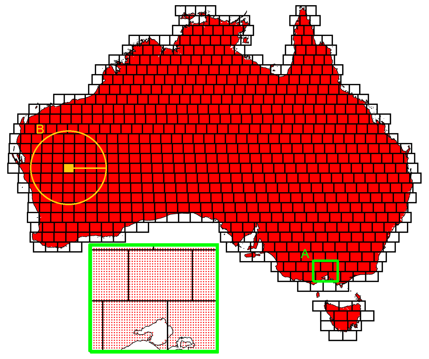
Figure 2The GRACE GSFC Mascon grid (black rectangles) and the CABLE 0.05∘ grids (red dots) in Australia. The green inset shows details of rectangle A. The orange circle B shows the number of mascon cells inside a ∼3∘ radius, which are used to update the state variables inside the center mascon (filled orange). Processing details can be found in Sect. 3.1.
2.4 Evaluation data
2.4.1 Satellite-derived products
The satellite-derived soil moisture and evapotranspiration (ET) data obtained from the European Space Agency Climate Change Initiative program (ESA CCI; Dorigo et al., 2017; Gruber et al., 2019) and the Global Land Evaporation Amsterdam Model (GLEAM; Martens et al., 2017) are used to validate the soil moisture and evaporation estimates, respectively. The ESA CCI COMBINED product combines multiple active and passive satellite sensor soil moisture products and provides a near-global daily volumetric soil moisture product at 0.25∘ resolution with ∼0.04 m3 m−3 accuracy (unbiased root mean square error). The combined product version 4.7 (v04.7) is used in this study. The product includes approximately eight different satellite observations, including, e.g., SSM/I, AMSR-E, ASCAT, Windsat, and SMOS (see, e.g., Fig. 3 of Dorigo et al. (2017) for complete details) during our evaluation period (1981–2012). GLEAM is an algorithm that derives the daily global terrestrial evaporation using observations from multiple satellite microwave sensors and reanalysis data sets (Martens et al., 2017). In total, two product variants are available, i.e., the satellite-only and the reanalysis, and the newest release of the latter (version 3.3a) is used in this study due to its consistent time span with our evaluation period.
2.4.2 In situ data
In situ soil moisture, groundwater, and ET measurements are obtained from different ground observation networks. The daily in situ soil moisture data are obtained from the Scaling and Assimilation of Soil Moisture and Streamflow (SASMAS; Rüdiger et al., 2007) network in the southeastern part of the Murray–Darling Basin (see Fig. 1). The SASMAS network hosts more than 20 measurement sites and provides volumetric soil moisture (θ; m3 m−3) data associated with 0–5 cm depth. Only sites with a data record longer than 3 years are used in our analysis.
The monthly in situ groundwater level data are collected from the Australian Bureau of Meteorology through the Australian Groundwater Explorer. More than 870 000 monitoring bores are distributed across the continent. At each bore, the groundwater level measurement is converted to the groundwater level variation by removing the long-term mean associated with the entire data record. The bores are excluded from the analysis if the data record is shorter than 3 years or has significant missing data. The groundwater level measurements are not converted to groundwater storage due to the absence of accurate knowledge of specific yield.
The in situ ET (i.e., latent heat flux) is obtained from the FLUXNET2015 data set (Pastorello et al., 2017). FLUXNET is a global network measuring carbon and energy fluxes. More than 20 flux tower sites are distributed across Australia and are associated with different periods (e.g., 2001–2014). Only the sites with 3 years of data or longer are used in our analysis (see site locations in Fig. 1a).
3.1 Ensemble Kalman smoother (EnKS)
The ensemble Kalman smoother (EnKS; Zaitchik et al., 2008) is used to assimilate the GRACE-derived ΔTWS into the CABLE model. The 3-dimensional EnKS (EnKS 3D) scheme described in Tangdamrongsub et al. (2017) is used in this study for two reasons. First, it accounts for spatial correlations in model and observation errors. The latter are highly correlated at neighboring or grid cells. Second, EnKS does not require interpolation of the observations (as in the ensemble Kalman filter (EnKF); Tangdamrongsub et al., 2015) and mitigates the spurious jump in water storage estimates caused by applying updates at the end of the month only. The additional computational cost is small, for handling large covariance matrices and running the model twice for each month.
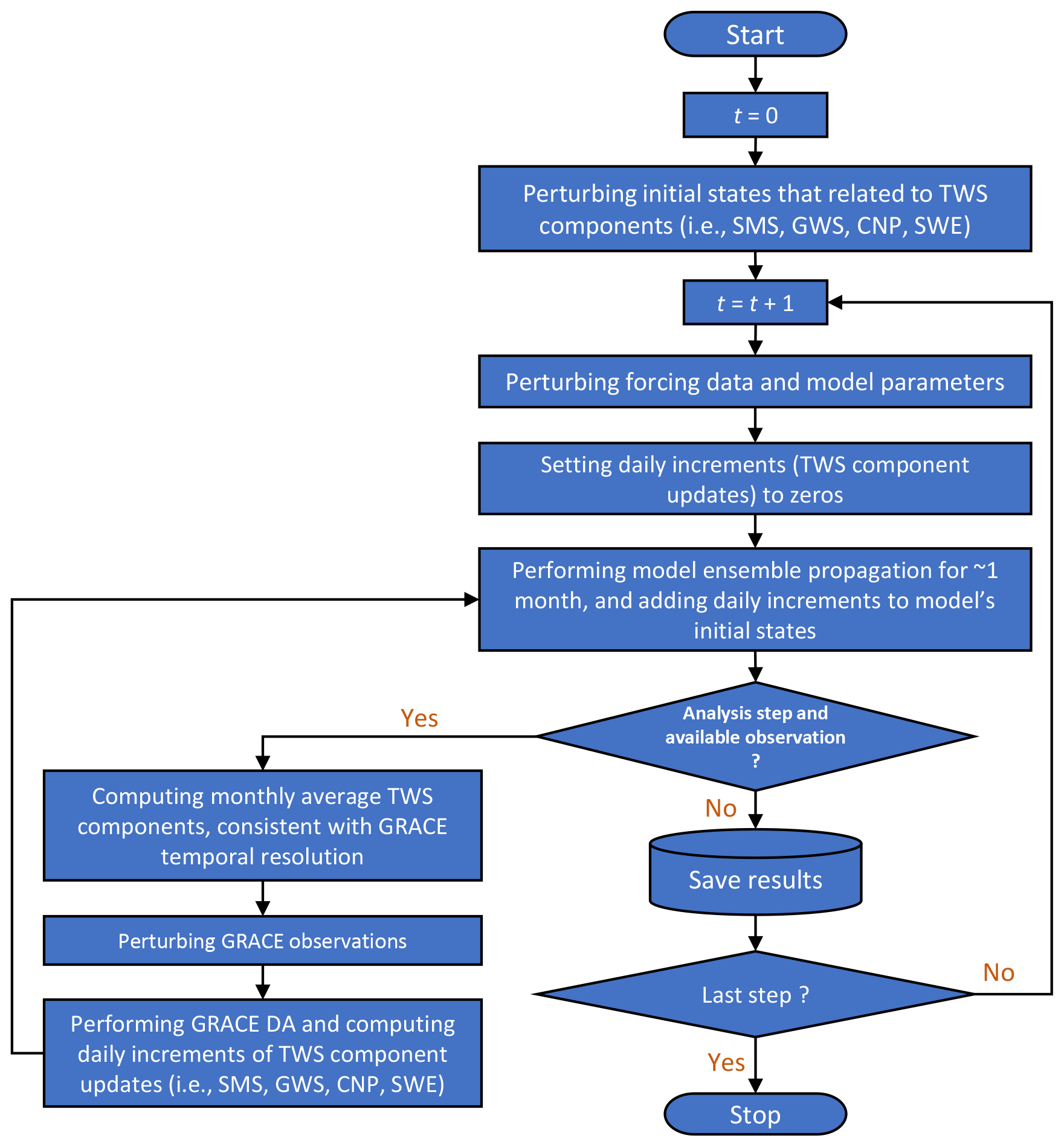
The GRACE DA comprises forecast, analysis, and distributing update steps. The forecast step propagates the model states forward in time for approximately 1 month. The analysis step computes the monthly model state update using GRACE observations (and uncertainties). The final step reinitializes the ensemble (e.g., initial states and forcing data) and reperforms the forecast step with the DA update (increment) distributed evenly throughout the month. Figure 3 illustrates the concept of the GRACE DA process. Pseudocodes of GRACE DA can be found in the Supplement.
Table 3Perturbation settings associated with the meteorological forcing data and model parameters. The comprehensive description of model parameters can be found in, e.g., Decker (2015) and Ukkola et al. (2016). The spatial correlation error is also applied to forcing data (fourth column). The correlation length of the 0.5 and 0.05∘ CABLE model (C05 and C005) is determined based on covariance analysis (see Sect. 3.2.4).
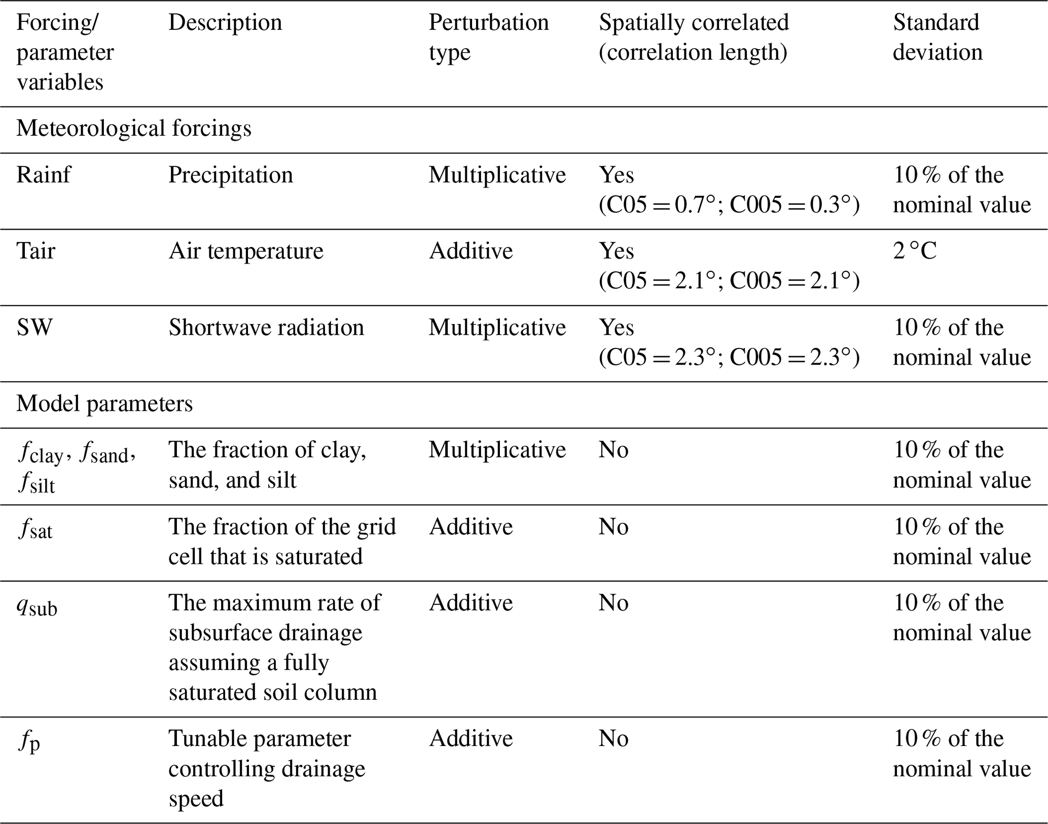
The meteorological forcings and model parameters are perturbed using N=100 ensemble members prior to GRACE DA processing. Multiplicative white noise is used to perturb the precipitation and shortwave radiation, while additive white noise is used for the air temperature and model parameters. The characteristics of the uncertainties are given in Table 3. Downscaling and upscaling forcing data also cause errors. In our DA process, when the data are resampled, their errors are also adjusted. The relationship between coarse and fine-scale errors can be expressed as follows:
where σc and σf represent coarse and fine-scale errors, (h, l) is the index of a grid cell, M is the number of fine-scale grid cells used in resampling, ϕ is a spherical distance between grid cells, and ϕ0 is the considered correlation length (e.g., a coarse scale's grid size). After the perturbation process, CABLE model states are then propagated for approximately 1 month (the forecast step). The state vector consists of nine model states (n=9), including six soil moisture layers, canopy storage, snow water equivalent, and groundwater storage.
In the analysis step, when a GRACE observation is available, the monthly averaged states (ψ) are related to the GRACE observations by the following:
where dj is an m×1 perturbed observation vector containing the perturbed GRACE mascon for the month of interest, H is a measurement operator which relates the ensemble state ψj to the vector dj, m is the number of GRACE mascon cells used in the calculation, and j indicates ensemble index. The uncertainties in the observations are described by the random error ϵ, which is assumed to have zero mean and covariance matrix Rm×m. The subscription denotes the dimension of the matrix. Note that R is a variance matrix here as only the variance components are provided in the mascon product.
In EnKS 3D, multiple model and observation grid cells (e.g., inside 300 km radius corresponding to GRACE spatial resolution) are simultaneously used to compute the state update. Figure 2 (see circle B) demonstrates the model and mascon grid cells used in the analysis step to compute the update of the center mascon cell (see also Fig. 7 of Tangdamrongsub et al. (2017) for more details). The H matrix is defined as follows:
where ki is the number of model grid cells inside a mascon i (see, e.g., rectangle A in Fig. 2 for the distribution of model grids inside a mascon cell).
The ensemble of the states is stored in a matrix , where , and the ensemble perturbation matrix is defined as , where the matrix contains the mean values computed from all ensemble members. Similarly, the perturbed GRACE observation vector is stored in the matrix . The analysis equation is then expressed as follows:
with
where represents the updated state vector, ΔAK×N is the monthly averaged update from EnKS 3D, and KK×m is the Kalman gain matrix. The superscript “T” denotes a transpose (matrix) operator. The model and observation error covariance matrix (Pe)K×K, (Re)m×m are computed as follows:
where Υ contains the measurement error of all ensemble members. After the monthly averaged update ΔA is obtained, the daily increment (ΔAd) of the update is computed by dividing ΔA by the total number of days in that month. Note that only ΔAd of the center mascon is saved (see also Tangdamrongsub et al., 2017). The processes described in Eqs. (2)–(7) are repeated through all mascon cells to obtain all individual ΔAd in the study domain. Then, the model is reinitialized using the previous month's initial states, and the simulation is performed again while adding ΔAd to the model initial states daily (the distributing update step). The DA process is performed until the last month of the study period (December 2012).
3.2 Assessment metrics and experiment designs
3.2.1 Resample approach
The state estimates are validated against the referenced data described in Sect. 2.4. As the spatial resolution of the model estimate and referenced data are different, a spatial resample is performed before the comparison. The model estimate is resampled to the observation grid space using the nearest-neighbor gridded interpolation when the model's resolution is coarser. Conversely, the estimate is upscaled (spatial averaging) when the model's resolution is higher. The evaluation is conducted at the observation grid cell.
3.2.2 Correlation and root mean square difference
The agreement between the estimated variable and the in situ data is assessed using the Pearson correlation coefficient (ρ) and the root mean square difference (RMSD). At a particular grid cell, ρ is calculated as follows:
where the y vector contains the model estimates, the x vector contains the validation data (observations), E[ ] is the expectation operator, and (, ), and (σy, σx) are the mean and standard derivations of y and x, respectively. The RMSD is computed as follows:
where L denotes the length of the time series.
3.2.3 Long-term trend and seasonal variations
The long-term trend, annual amplitude, and phase of the time series are computed using the least-squares adjustment associated with five parameters, offset (a), long-term trend (b), annual variation (c, d), and semi-annual variation (e, f). A time series (y) at a particular grid cell can be expressed as follows:
where the t vector contains time, and T is an annual period. The annual amplitude (A) and phase (φ) are computed as follows:
3.2.4 Spatial resolution
Spatial resolution is defined as the minimum distance at which two signals of equal magnitude can be separated. The spatial resolution can be determined from the empirical (and isotropic) covariance function (C) computed as follows (Tscherning and Rapp, 1974):
where (ph, pl) are vectors containing data points (h, l) associated with the spherical distance ϕhl, and nhl is the number of data pairs considered in the calculation. The spatial resolution (or correlation length of the covariance function) is defined in this study as being the distance ψ at which C(ϕ=0) decreases by half. The diagram in Fig. 4 illustrates how this correlation length is determined.
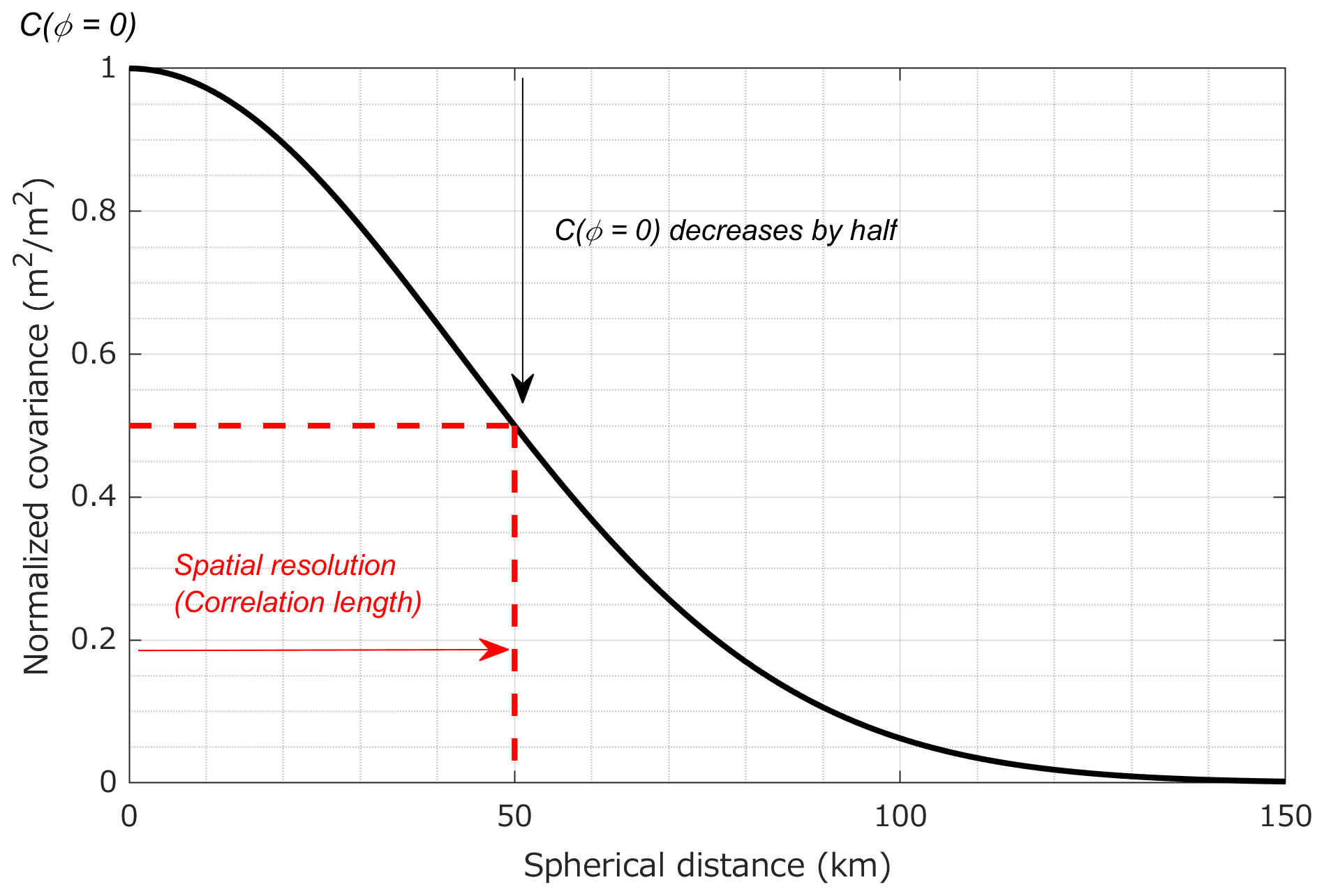
Figure 4The concept used to determine spatial resolution (correlation length). The spatial resolution is defined to be the spherical distance ϕ at which the 0 km covariance (or normalized covariance), C(ϕ=0) decreases by half.
3.2.5 Case studies
This paper uses four case studies to quantify the effect of different model grid sizes and GRACE DA. The case studies are described as follows:
-
CABLE 0.5∘ – CABLE model simulations at 0.5∘ grid size without GRACE DA;
-
CABLE 0.05∘ – CABLE model simulations at 0.05∘ grid size without GRACE DA;
-
GRACE DA 0.5∘ – CABLE model simulations at 0.5∘ grid size with GRACE DA;
-
GRACE DA 0.05∘ – CABLE model simulations at 0.05∘ grid size with GRACE DA.
It is noteworthy that the 0.5 or 0.05∘ represents the CABLE grid size, which may differ from the spatial resolution. The term “spatial resolution”, as used in this paper, refers to the determined resolution computed from Sect. 3.2.4.
4.1 Estimation of TWS components from CABLE simulations (without GRACE DA)
4.1.1 Improvement in spatial resolution
The resolution improvements can be seen by comparing CABLE 0.5∘ TWS estimates against those from CABLE 0.05∘. Both are open-loop (OL) simulations, meaning the model is run without data assimilation. The simulation period is from January 1981 to December 2012. After obtaining TWS estimates, the TWS annual amplitude and phase are computed using Eqs. (12) and (13) and are shown in Fig. 5. Both CABLE versions have similar spatial features, but more localized and much finer details are seen in the CABLE 0.05∘ simulation than in the CABLE 0.5∘ simulation. A clear difference in annual amplitude is shown over the Yarra Ranges and the Alpine National Park (compare Fig. 5a vs. Fig. 5b insets). CABLE 0.05∘ provides greater details of the ΔTWS spatial distribution, and the annual amplitude is approximately 30 % higher than it is in the coarse-scale version. Differences in spatial details are also seen in the phase estimates (see Fig. 5c vs. Fig. 5d).
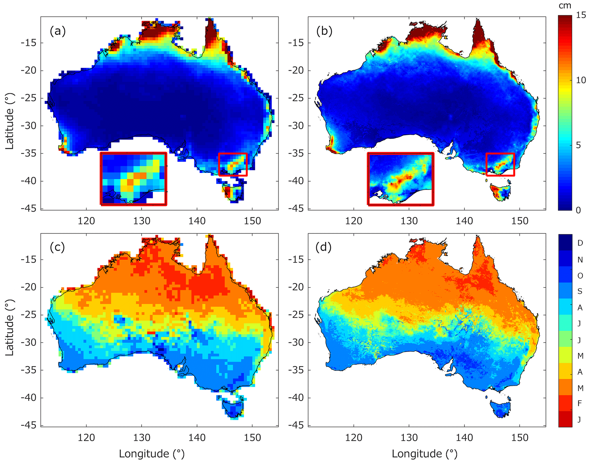
Figure 5Annual amplitude (a, b) and phase (c, d) of the TWS estimates computed from CABLE 0.5∘ (a, c) and CABLE 0.05∘ (b, d). The insets in (a) and (b) show details in southeastern Australia. The phase exhibits the timing when TWS reaches the maximum value (with respect to the beginning of the year). The unit of the phase is a calendar month, e.g., January (J) or December (D).
The spatial resolutions can be quantitatively determined using the empirical covariance function, Eq. (14), described in Sect. 3.2.4. The covariance function is computed for each month's TWS estimates using all grid points in Australia. Figure 6 shows the averaged spatial resolution (correlation length) of CABLE 0.5∘ and CABLE 0.05∘ for each month between 1981 and 2012. The CABLE 0.5∘ simulations have a spatial resolution of ∼50 km, consistent with the grid size of the input 0.5∘ CABLE parameters and forcing data. Larger correlation lengths are found during the rainy seasons (January–April in the north and August–November in the south) and during the dry season (e.g., June). Soil moisture and aquifer storage increase during the wet seasons, leading to more uniform (and smoother) spatial moisture features. Similar uniformity can also be observed during the dry season. At the beginning of the wet season, scattered rainfall in part of the continent likely causes a gradient between dry/wet areas, resulting in smaller correlation lengths. It is noteworthy that our analysis only explains the overall temporal pattern of continental correlation lengths. The temporal pattern may also be affected by the local TWS wet/dry features or by the spatial distribution of model parameters.
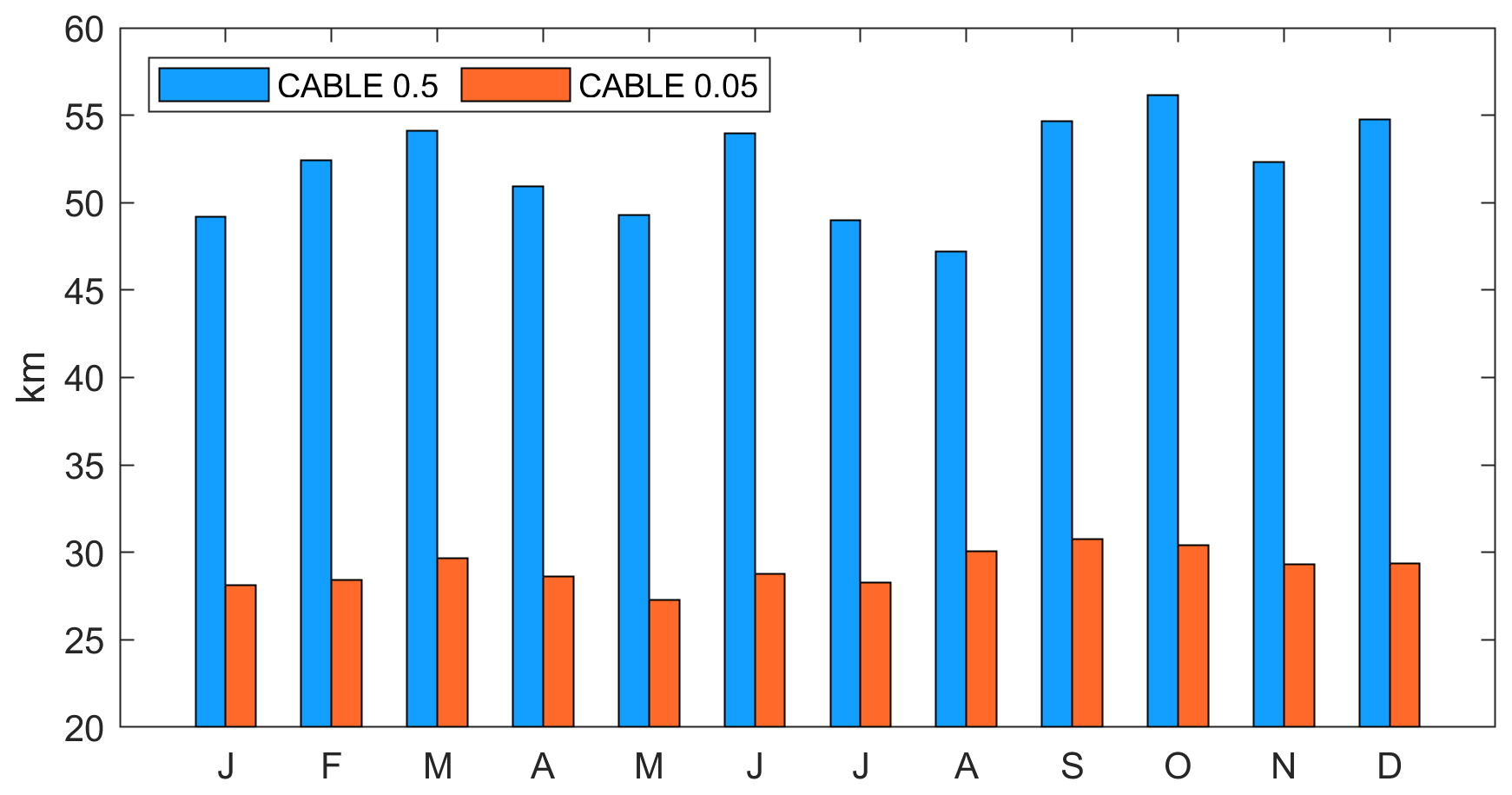
Figure 6Monthly average spatial resolutions (correlation lengths) of the TWS estimates derived from CABLE 0.5∘ and CABLE 0.05∘ in Australia between 1981 and 2012.
The use of CABLE 0.05∘ significantly improves the spatial resolution by about a factor of 2 to 3. Note, again, that the spatial resolution of CABLE 0.05∘ presented in Fig. 6 reflects the continental averaged value while the finer (higher) spatial resolution is observed in the individual river basin (not shown).
4.1.2 Assessment of long-term TWS variations
This study's time span allows for an assessment of overall trends and decadal variations in TWS estimates. The long-term trends of water balance states and fluxes from CABLE 0.05∘ between 1981 and 2012 are shown in Fig. 7. A strong relationship between components is observed, particularly in the storage components (Fig. 7a–d). The TWS and GWS (Fig. 7a and d) have very similar spatial patterns, where a wetting trend is observed in the northern region, the Indian Ocean basin, and the western part of the Murray–Darling Basin (see Fig. 1a for the basin's location), and a drying trend is seen in the central part of the continent, the South West Coast basin, and several parts of the Murray–Darling Basin. The similarity between the TWS and GWS (both spatially and in magnitude) indicates that GWS is a primary driver of the TWS trend in Australia. By contrast, soil moisture stores show different spatial patterns; increases in soil moisture are also found in the central and western parts of the continent (Fig. 7c). The SMS generally accommodates a large portion of the seasonal variation in water storage in Australia (see Sect. 4.2), but its role in the long-term trend is marginal – smaller than that of the GWS by about a factor of 2. ET trend estimates show a similar spatial pattern to SSM trends (Fig. 7e vs. Fig. 7b), which may be explained by ET pulling moisture from SSM stores. The long-term trend of the total runoff is in line with the TWS/GWS, increasing in the north and decreasing in the southeastern region and Tasmania (e.g., Fig. 7f vs. Fig. 7a). In the northern region, the soil moisture or aquifer is likely saturated due to a wet climate, with more significant annual rainfall (than the south) by about a factor of 5 (not shown). Such a condition leads to a greater magnitude of root zone moisture, groundwater recharge, and surface runoff variations. The opposite scenario is observed in the southeastern region, where the depleted TWS/GWS (induced by droughts) likely reduces runoff generation, resulting in a negative runoff trend.
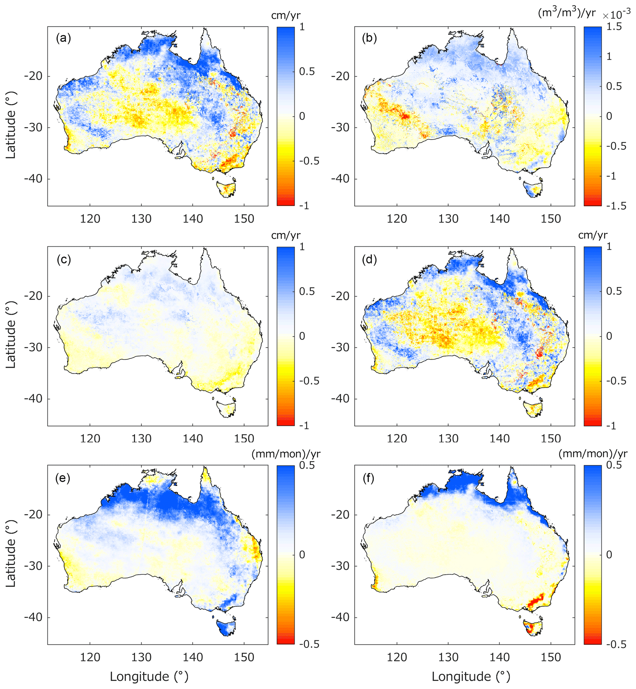
Figure 7Long-term trends computed from CABLE 0.05∘ between January 1981 and December 2012, showing the (a) terrestrial water storage (TWS), (b) surface (volumetric) soil moisture (SSM), (c) total soil moisture storage (SMS), (d) groundwater storage (GWS), (e) evapotranspiration (ET), and (f) total runoff.
Regional water balance components can also be analyzed at interannual and decadal timescales. Figure 8 shows the trends of water balance components in 3 different decades, i.e., 1981–1990, 1991–2002, and 2003–2012. The long-term trends are not monotonic. In other words, there are no “always dry” or “always wet” regions observed between 1981 and 2012. Reversals between increasing and decreasing trends are apparent in all components. For example, northern and western Australia experience a drying trend between 1981 and 1990 (Fig. 8a) and recover between 1991 and 2002 (Fig. 8b) after continuously receiving increased rainfall (not shown). The region experiences another drought episode (van Dijk et al., 2013a) in the first half of the 2000s, causing decreased water storage between 2003 and 2012 (Fig. 8c). A similar reversal is also seen in the eastern regions, with wetting in 1981–1990, drying in 1991–2002, and wetting again in 2003–2012 (Fig. 8a–c).

Figure 8Similar to Fig. 7 but the trends are associated with three different periods, i.e., 1981–1990 (a, d, g, j, m, p), 1991–2002 (b, n, h, k, n, q), and 2003–2012 (c, f, i, l, o, r).
Without such a long record, assessment of water resources may have limited reliability. For instance, based only on the ∼10-year period of GRACE observations, it is difficult to determine whether the negative TWS trend in western Australia (e.g., Fig. 8c; see also Fig. 11d) is caused by anthropogenic or natural processes (e.g., Richey et al., 2015). Evaporation or runoff after the extremely wet conditions prior to 2002 may also produce a similar decreasing trend (e.g., van Dijk et al., 2011; Munier et al., 2012). By assessing the historical TWS time series of the North Western Plateau basin obtained from CABLE 0.05∘ (Fig. 9), the observed negative trend is more likely governed by a decadal cycle of drought and recovery. This approach demonstrates that there is clear value in utilizing a longer time span of TWS estimates, and that this can offer a more reliable assessment of regional water resources and climate variations.

Figure 9The TWS estimates of the Sandy Desert basin obtained from CABLE 0.05∘ between January 1981 and December 2012. The long-term trend estimates (centimeters per year) in different periods are given. The blue highlight indicates the GRACE period (January 2003–December 2012).
4.1.3 Comparison with the satellite products
TWS, SSM, and ET estimates are compared with satellite data from GRACE, ESA CCI, and GLEAM, respectively (see Sect. 2.2 and 2.3 for each product's description). Note that the remote sensing products may contain biases (caused by, e.g., background model and processing algorithm) and do not necessarily represent the truth. (Ground truth validation is performed in Sect. 4.3.) The intercomparison performed in this section is only to assess the consistency between two independent estimates, i.e., model and satellite. The CABLE estimate is rescaled to the satellite product's grid before comparison, as described in Sect. 3.2.1. Figure 10 shows the correlation and RMSD estimates between CABLE 0.5∘ and CABLE 0.05∘ results and the evaluated satellite data. On average, both CABLE results are in good agreement with the satellite products, with correlation values greater than 0.55 (see Fig. 10a, b, e, f, i, j). CABLE 0.05∘ shows a more robust agreement with satellite-derived variables than CABLE 0.5∘ does; correlation values with TWS, SSM, and ET are 14 %, 14 %, and 7 % higher (respectively) in the former simulations than in the latter. Similar improvements are also observed in the RMSD evaluations, where CABLE 0.05∘ provides smaller RMSD values than CABLE 0.5∘ by 4 % (TWS), 14 % (SSM), and 17 % (ET). CABLE 0.05∘ reduces the RMSD of the SSM estimate to as low as ∼0.03 m3 m−3, e.g., over the South West Coast and Lake Eyre basins, and the average RMSD value in Australia is ∼0.06 m3 m−3. It is worth noting that the average unbiased RMSD value (Entekhabi et al., 2010b) is 0.037 m3 m−3 (not shown), in line with the accuracy of the CCI product (see, e.g., Table 1 of Dorigo et al., 2017).
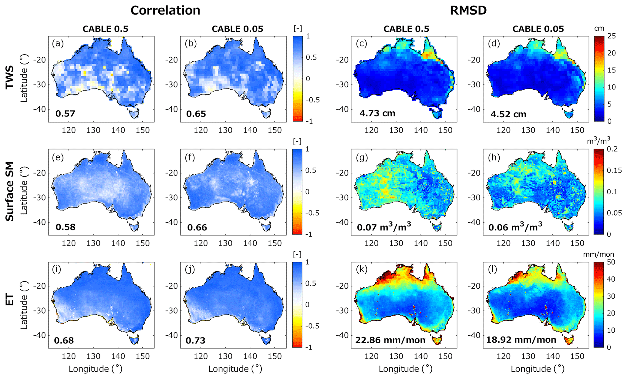
Figure 10The comparison between CABLE 0.5∘ and CABLE 0.05∘ estimates and different remote sensing products in terms of correlation coefficient (a, b, f, i, j) and root mean square difference (RMSD; c, d, g, h, k, l). The terrestrial water storage (TWS; a–d), surface soil moisture (SSM; e–h), and evapotranspiration (ET; i–l) are compared with GRACE, ESA CCI, and GLEAM products, respectively. The averaged statistical values (over Australia) associated with each comparison are also given.

Figure 11The change in terrestrial water storage (ΔTWS; a–c), surface soil moisture (SSM; d–f), and evapotranspiration (ET; g–i) estimated from CABLE 0.5∘ (CB0.5), CABLE 0.05∘ (CB0.05), and remote sensing observations (Obs) over three different river basins, i.e., North Western Plateau (a, d, g), Lake Eyre (b, e, h), and South West Coast (c, f, i), between 1981 and 2012. The remote sensing observations used for comparison are GRACE (TWS), ESA CCI (SSM), and GLEAM (ET).
The improved agreement between CABLE 0.05∘ estimates and the satellite products is also seen in the temporal variation (Fig. 11). Compared with the CABLE 0.5∘ results, CABLE 0.05∘ increases the dynamic range of the TWS estimates in most basins, leading to closer alignment with GRACE observations (Fig. 11a–c). Similar increases in the agreement are also observed in the CABLE 0.05∘ SSM and ET estimates (Fig. 11d–i). The observed improvement may be attributed, in part, to the rederived model parameters. For example, in the North Western Plateau basin, CABLE 0.05∘ uses a ∼17 % higher area-averaged sand fraction than CABLE 0.5∘ does, which allows faster infiltration/drainage in the storage compartments, leading to greater dynamic ranges of TWS and SSM variations (see Fig. 11a and d). Consequently, the ET estimate is decreased as a response to increased water storage following the water balance equation (Fig. 11g). Similar mechanisms are also observed in the Lake Eyre and South West Coast basins, where the improved parameterization leads to improved agreement with the satellite data. The use of coarse-resolution forcing data (e.g., precipitation) could also explain the small TWS amplitude observed in CABLE 0.5∘. Coarse-scale forcing data averages local precipitation signals over a larger area than the finer-resolution forcing data does, resulting in a smaller amplitude.
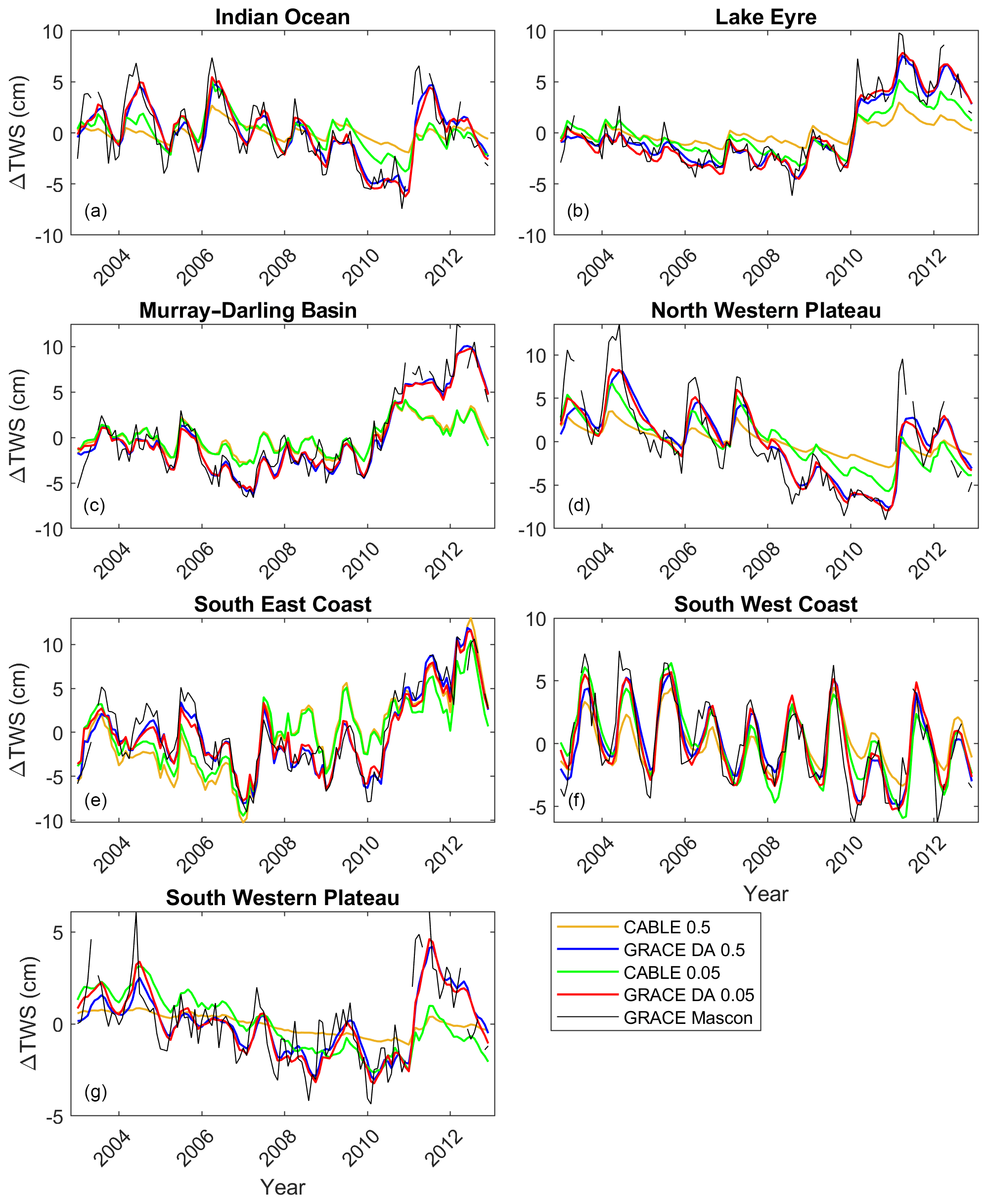
Figure 12The TWS estimates from case studies CABLE 0.5∘, CABLE 0.05∘, GRACE DA 0.5∘, and GRACE DA 0.05∘ in various river basins between 2003 and 2012. The GRACE observation is also displayed for comparison. Full descriptions of the case studies are given in Sect. 3.2.5.
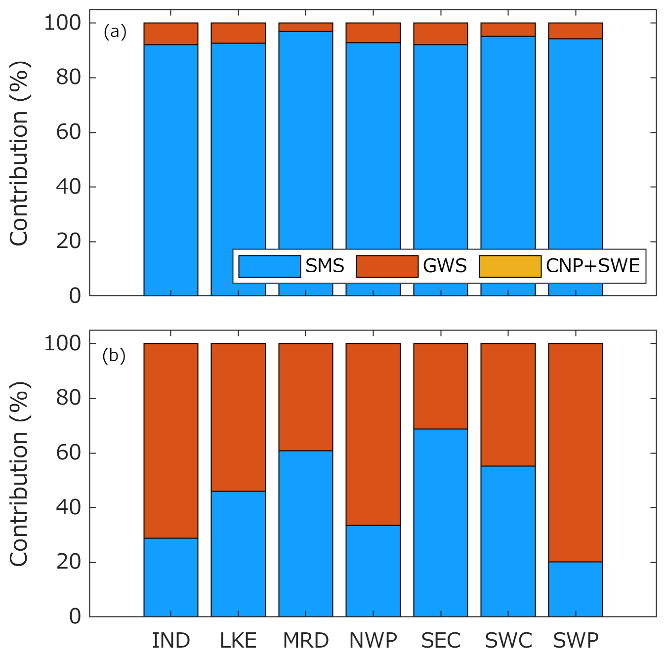
Figure 13Contributions of different storage components (total soil moisture storage – SMS; groundwater storage – GWS; canopy storage – CNP; and snow water equivalent – SWE) to the TWS estimates computed from CABLE 0.05∘ (a) and GRACE DA 0.05∘ (b) in different river basins. The full names of the river basins are given in Fig. 1a. Contributions of CNP + SWE are negligible in both panels.
4.2 The impact of GRACE DA
GRACE observations are assimilated into the CABLE 0.5∘ and CABLE 0.05∘ models (called GRACE DA 0.5∘ and GRACE DA 0.05∘, respectively) between January 2003 and December 2012 (due to the availability of meteorological forcing and GRACE data). The basin-averaged TWS estimates from CABLE with and without GRACE DA are shown in Fig. 12, alongside the GRACE observations themselves. In most basins, apparent disagreements between the open-loop estimates and the GRACE observations suggest the current CABLE models' limited accuracy. After assimilating GRACE into the models, the estimates (GRACE DA 0.5∘ and GRACE DA 0.05∘) move toward the GRACE observations. The positive impact of GRACE DA on the basin-averaged TWS estimates is similar regardless of the model spatial resolutions. This likely reflects the nature of GRACE observations that provide integrated water storage information at the continental or basin scale (Tapley et al., 2004). However, it should be noted that the GRACE DA application does not degrade the spatial resolution of the model. The offline analysis shows that the average correlation length of GRACE DA 0.5∘ and GRACE DA 0.05∘ remain the same as that of CABLE 0.5∘ and CABLE 0.05∘, respectively (not shown). The EnKS 3D scheme exploits the spatially correlated information from the high-resolution model to disaggregate the coarse-scale observations into a finer grid space, resulting in the preservation of the model's intrinsic resolution. The impact of GRACE DA is also observed in water redistribution within the water storage components. Figure 13 shows the contributions of four different water storage components (SMS, GWS, SWE, and CNP) to TWS in different basins before (CABLE 0.05∘; Fig. 13a) and after the application of GRACE DA (GRACE DA 0.05∘; Fig. 13b). The contribution is calculated as a percent of the annual amplitude of TWS fluctuations. In CABLE 0.05∘ (Fig. 13a), the SMS is a major contributor to more than 90 % of the TWS variation (i.e., annual amplitude). The GWS contribution is only ∼10 %. After applying GRACE DA (Fig. 13b), the contribution of the GWS is significantly increased. It dominates the entire water column in several basins (e.g., Indian Ocean, Lake Eyre, North West Plateau, and South West Plateau). This behavior reflects the nature of GRACE in that the groundwater provides a majority of the seasonal changes to terrestrial water mass. GRACE DA has been shown to significantly affect GWS in previous studies (e.g., Girotto et al., 2016; Tangdamrongsub et al., 2018; Li et al., 2019). The contributions of the SWE and CNP components are negligible across Australia, and the impact of GRACE DA on them is trivial. Similar changes to TWS contributions are also observed between CABLE 0.5∘ and GRACE DA 0.5∘ (not shown). It is noted that Figs. 12 and 13 only present the impact of GRACE DA on storage components and do not assess the accuracy of either version. The accuracy of the OL and DA models is quantified in Sect. 4.3.
4.3 Validation with in situ data
In situ data from three different ground networks (see Sect. 2.3.2) are used to validate the GWS, ET, and SSM estimates. Validation is conducted by quantifying the change in correlation values between simulations and observations when one model is used in place of another. The validation period is between January 2003 and December 2012, consistent with the GRACE DA period. Figure 14 shows the validation of GWS estimates between GRACE DA and OL simulations (DA minus OL). A positive value indicates improvement, while a negative value represents degradation. A significance test is performed at the 0.05 level based on the Fisher Z transformation test for correlation coefficients (Zaitchick et al., 2008). The average change in correlation value across all in situ data sites is shown in Fig. 14d. Values that failed the significant test are excluded from the averaging.

Figure 14(a–c) Improvements or degradations in correlation values between case study simulations (Sect. 3.2.5) and in situ observations of GWS estimates. (a) GRACE DA 0.5∘ minus CABLE 0.5∘, (b) GRACE DA 0.05∘ minus CABLE 0.05∘, and (c) GRACE DA 0.05∘ minus GRACE DA 0.5∘. The relative performance of each simulation is indicated with blue/red shading. Blue indicates that the first simulation is better than the second, and red indicates that the second is better than the first. Changes that are not significant at the 0.05 level are displayed in gray. (d) The average change in correlation value from each scenario is the vertically displayed case study minus the horizontally displayed case study (e.g., d1 represents GRACE DA 0.5∘ minus CABLE 0.5∘ and indicates that the former is significantly better than the latter).
We first analyze the impact of GRACE DA on the GWS estimates of CABLE 0.5∘ and CABLE 0.05∘ (Fig. 14a and b). A greater correlation improvement is observed when GRACE DA is applied to the 0.5∘ model, which increases the average correlation value by 0.23 (Fig. 14d1). When GRACE DA is applied to the 0.05∘ model (Fig. 14b), the average correlation value improves by 0.12 (Fig. 14d6), which is ∼50 % less than in the 0.5∘ model.
When comparing the two OL runs (CABLE 0.5∘ vs. CABLE 0.05∘), the GWS estimate from CABLE 0.05∘ has a higher correlation value by 0.12 (see Fig. 14d2). This analysis indicates that the lower correlation improvement seen between CABLE 0.05∘ and GRACE DA 0.05∘ is unlikely caused by the reduced impact of GRACE DA on the high-resolution model. Rather, it is a result of CABLE 0.05∘ having better accuracy to start with. GRACE DA tends to provide the same information to both 0.5 and 0.05∘ models. Still, GRACE DA 0.05∘ exhibits the best correlation with in situ data, ∼0.02 higher than GRACE DA 0.5∘ (Fig. 14c and d5). While GWS estimates from both CABLE 0.5∘ and CABLE 0.05∘ improve with GRACE DA, we find that GRACE DA 0.5∘ (DA) shows a higher correlation value than CABLE 0.05∘ (OL) by 0.1 (see Fig. 14d3). This indicates that improving model state estimates via DA is more effective than improving model parameters via increased resolution. Despite different study areas, LSMs, and validation data, our finding is in line with, e.g., Girotto et al. (2017) and Nie et al. (2019), who also found a significant impact of GRACE DA on GWS components.
SSM and ET estimates are validated against ground measurements from SASMAS and Ozenet, respectively. Correlation coefficients between the case study simulations and observation networks are summarized in Fig. 15. For SSM (Fig. 15a), CABLE 0.05∘ exhibits slightly improved correlation with observations (by ∼0.6 %) than CABLE 0.5∘ does. The addition of GRACE DA also shows a small but positive impact on SSM estimates, improving correlation with observations by ∼1 %. The small impact is attributed to limited GRACE sensitivity. GRACE is sensitive to the low-frequency variation (originated from deeper stores) and cannot effectively capture SSM, which is dominated by a high-frequency signal (e.g., precipitation). As a result, GRACE DA is found to have a minor (or negative) impact on the top soil component in most GRACE DA studies (e.g., Li et al., 2012; Tian et al., 2017; Tangdamrongsub et al., 2020). The small impact on SSM estimates also agrees with Jung et al. (2019), who observed GRACE DA's small (or negative) impact over dry regions in West Africa.
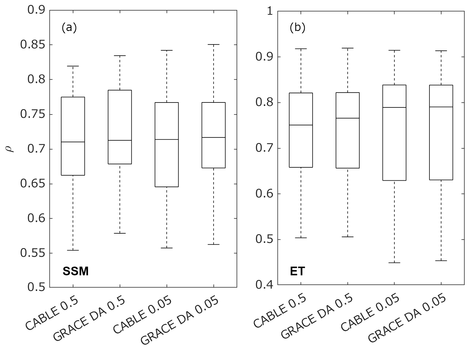
Figure 15Box and whisker plots showing correlation values between (a) simulation case studies and in situ surface soil moisture and between (b) simulations and evapotranspiration estimates.
For ET (Fig. 15b), CABLE 0.05∘ exhibits a more improved correlation with observations (by ∼5 %) than CABLE 0.5∘ does. The inclusion of GRACE DA also slightly improves correlation values over the associated OL model versions. Greater improvement (by ∼2 %) is seen between CABLE 0.5∘ and GRACE DA 0.5∘ than between CABLE 0.05∘ and GRACE DA 0.05∘. As with SSM, the small improvement of ET is likely attributable in part to small GRACE DA updates (caused by the limited GRACE sensitivity to high-frequency surface fluxes). The SSM is a primary moisture source for ET, so a trivial change in SSM leads to a similarly small change in ET.
This study enhances the spatial resolution and time span (>30 years) of regional TWS estimates using the CABLE LSM, high-resolution land cover maps and forcing data, and GRACE DA application. By improving the model parameter and forcing data (without GRACE DA), the developed CABLE 0.05∘ model shows clear improvements in the accuracy of water balance component estimates (e.g., soil moisture, groundwater, and evapotranspiration) when compared with in situ and independent satellite data. The 0.05∘ model also improves the spatial resolution by a factor of 2 to 3 over the 0.5∘ version. The extended time span provides insightful information for long-term assessment of regional water resources and climate variability. The enhanced model parameterization is found to play a significant role in the improved TWS estimates. Incorporating GRACE DA into the model leads to further improvements in TWS component estimates. The positive impact of GRACE DA is found in the deep storage component (e.g., GWS), while the impact on the surface components and flux estimates (i.e., SSM and ET) is trivial. Of the four case studies investigated here, the most accurate simulation uses CABLE 0.05∘ with GRACE DA.
The enhanced CABLE model resolution developed in this study relies on improved parameter and forcing data. The land surface physics remains unchanged. The workflow can be adopted for other CABLE repositories or different LSMs with only slight modifications, e.g., number of soil or vegetation types. This means TWS estimates can be reproduced with more spatial detail by CABLE 0.05∘ at locations outside the area studied here since high-resolution forcing data and model parameters are available globally (or near globally). However, the performance of such simulations might differ from this study due to the uncertainty in model parameters and forcing data that vary with geolocations (e.g., Herold et al., 2017; Tifafi et al., 2018). This remark also applies to the performance of GRACE DA. Although the improvement of assimilating GRACE into CABLE is also seen in other regions, e.g., northeastern China (Yin et al., 2020), it is still difficult to quantify the benefit of GRACE DA over global river basins based on these early developments of CABLE and GRACE DA. Validation is highly encouraged to ascertain the accuracy of TWS estimates when performing the simulation in other regions.
Our development is only demonstrated between 1981–2012 due to the availability of the Princeton forcing data. Future development can consider extending the temporal record of TWS estimates. The time span extension is feasible using reanalysis forcing data from the Modern-Era Retrospective Analysis for Research and Applications, version 2 (MERRA-2; Gelaro et al., 2017). Despite a slightly coarser spatial resolution than the Princeton data, MERRA2 data sets would allow TWS simulations to be extended to the near present.
Pseudocodes of GRACE DA can be found in the Supplement.
The model and data used in this study are publicly available and can be accessed as follows (last access: 6 May 2020):
-
CABLE model, available at https://trac.nci.org.au/trac/cable (NCI, 2020)
-
The Harmonized World Soil Database version 1.2, available at http://www.fao.org/soils-portal/soil-survey/soil-maps-and-databases/harmonized-world-soil-database-v12/en (FAO, 2020)
-
The global land cover climatology using MODIS data, available at https://archive.usgs.gov/archive/sites/landcover.usgs.gov/global_climatology.html (USGS, 2020)
-
The Global Land Surface Satellite, available at http://www.glass.umd.edu (GLASS, 2020)
-
The Princeton forcing data, available at https://hydrology.princeton.edu/data.pgf.php (Terrestrial Hydrology Research Group, 2020)
-
The Climate Hazards Group InfraRed Precipitation with Station data, available at https://chc.ucsb.edu/data/chirps (University of California, 2020)
-
GRACE GSFC Mascon, available at https://earth.gsfc.nasa.gov/geo/data/grace-mascons (NASA, 2020)
-
The ESA CCI, available at https://www.esa-soilmoisture-cci.org (ESA, 2020)
-
The Global Land Evaporation Amsterdam Model, available at https://www.gleam.eu (GLEAM, 2020)
-
In situ soil moisture, available at https://ismn.geo.tuwien.ac.at/en (ISMN, 2020)
-
In situ groundwater, available at http://www.bom.gov.au/water/groundwater/explorer/map.shtml (Australian Government, 2020)
-
In situ evapotranspiration, available at https://fluxnet.fluxdata.org/data/fluxnet2015-dataset (FLUXNET, 2020)
-
ERA5, available at https://www.ecmwf.int/en/era5-land (ECMWF, 2020)
-
W3, available at http://wald.anu.edu.au/challenges/water/w3-and-ozwald-hydrology-models (Australian National University, 2020).
The supplement related to this article is available online at: https://doi.org/10.5194/hess-25-4185-2021-supplement.
NT conceptualized the paper, led the formal analysis, developed the software, validated, visualized, and wrote the original paper. MJ supervised the project and acquired the funding. PS assisted with the editing of the paper.
The authors declare that they have no conflict of interest.
Publisher's note: Copernicus Publications remains neutral with regard to jurisdictional claims in published maps and institutional affiliations.
We thank the three anonymous reviewers, Thom Bogaard, and HESS editorial team for their valuable suggestions, which helped us improve our paper significantly. Natthachet Tangdamrongsub thanks Mark Decker for the CABLE-SSGW model development.
This research was supported by the Earth Sciences Division in support of the National Climate Assessment.
This paper was edited by Thom Bogaard and reviewed by three anonymous referees.
Alkama, R., Decharme, B., Douville, H., Becker, M., Cazenave, A., Sheffield, J., Voldoire, A., Tyteca, S., and Le Moigne, P.: Global Evaluation of the ISBA-TRIP Continental Hydrological System. Part I: Comparison to GRACE Terrestrial Water Storage Estimates and In Situ River Discharges, J. Hydrometeorol., 11, 583–600, https://doi.org/10.1175/2010JHM1211.1, 2010.
Australian Goverment: Australian Groundwater Explorer, available at: http://www.bom.gov.au/water/groundwater/explorer/map.shtml, last access: 6 May 2020.
Australian National University: Environmental model software: W3 and OzWALD, available at: http://wald.anu.edu.au/challenges/water/w3-and-ozwald-hydrology-models, last access: 6 May 2020.
Beamer, J. P., Hill, D. F., Arendt, A., and Liston, G. E.: High-resolution modeling of coastal freshwater discharge and glacier mass balance in the Gulf of Alaska watershed, Water Resour. Res., 52, 3888–3909, https://doi.org/10.1002/2015WR018457, 2016.
Bi, D., Dix, M., Marsland, S., O'Farrell, S., Rashid, H., Uotila, P., Hirst, T., Kowalczyk, E., Golebiewski, M., Sullivan, A., Yan, H., Hannah, N., Franklin, C., Sun, Z., Vohralik, P., Watterson, I., Zhou, X., Fiedler, R., Collier, M., Ma, Y., Noonan, J., Stevens, L., Uhe, P., Zhu, H., Griffies, S., Hill, R., Harris, C., and Puri, K.: The ACCESS Coupled Model: Description, Control Climate and Evaluation, Aust. Meteorol. Oceanogr. J., 63, 41–64, https://doi.org/10.22499/2.6301.004, 2013.
Bierkens, M. F. P.: Global hydrology 2015: State, trends, and directions, Water Resour. Res., 51, 4923–4947, https://doi.org/10.1002/2015WR017173, 2015.
Bierkens, M. F. P., Bell, V. A., Burek, P., Chaney, N., Condon, L. E., David, C. H., Roo, A. de, Döll, P., Drost, N., Famiglietti, J. S., Flörke, M., Gochis, D. J., Houser, P., Hut, R., Keune, J., Kollet, S., Maxwell, R. M., Reager, J. T., Samaniego, L., Sudicky, E., Sutanudjaja, E. H., van de Giesen, N., Winsemius, H., and Wood, E. F.: Hyper-resolution global hydrological modelling: what is next?, Hydrol. Process., 29, 310–320, https://doi.org/10.1002/hyp.10391, 2015.
Bond, N. R., Lake, P. S., and Arthington, A. H.: The impacts of drought on freshwater ecosystems: an Australian perspective, Hydrobiologia, 600, 3–16, https://doi.org/10.1007/s10750-008-9326-z, 2008.
Broxton, P. D., Zeng, X., Sulla-Menashe, D., and Troch, P. A.: A Global Land Cover Climatology Using MODIS Data, J. Appl. Meteorol. Clim., 53, 1593–1605, https://doi.org/10.1175/JAMC-D-13-0270.1, 2014.
Castellazzi, P., Martel, R., Galloway, D. L., Longuevergne, L., and Rivera, A.: Assessing Groundwater Depletion and Dynamics Using GRACE and InSAR: Potential and Limitations, Groundwater, 54, 768–780, https://doi.org/10.1111/gwat.12453, 2016.
Crow, W. T., Berg, A., Cosh Michael, H., Loew, A., Mohanty, B. P., Panciera, R., Rosnay, P., Ryu, D., and Walker J. P.: Upscaling sparse ground-based soil moisture observations for the validation of coarse-resolution satellite soil moisture products, Rev. Geophys., 50, RG2002, https://doi.org/10.1029/2011RG000372, 2012.
Decker, M.: Development and evaluation of a new soil moisture and runoff parameterization for the CABLE LSM including subgrid-scale processes, J. Adv. Model. Earth Syst., 7, 1788–1809, https://doi.org/10.1002/2015MS000507, 2015.
Delworth, T. L. and Manabe, S.: The Influence of Potential Evaporation on the Variabilities of Simulated Soil Wetness and Climate, J. Climate, 1, 523–547, https://doi.org/10.1175/1520-0442(1988)001<0523:TIOPEO>2.0.CO;2, 1988.
Dong, B., Lenters, J. D., Hu, Q., Kucharik, C. J., Wang, T., Soylu, M. E., and Mykleby, P. M.: Decadal-scale changes in the seasonal surface water balance of the central U.S. from 1984–2007, J. Hydrometeorol., 21, 1905–1927, https://doi.org/10.1175/JHM-D-19-0050.1, 2020.
Dong, J. and Crow, W. T.: The Added Value of Assimilating Remotely Sensed Soil Moisture for Estimating Summertime Soil Moisture-Air Temperature Coupling Strength, Water Resour. Res., 54, 6072–6084, https://doi.org/10.1029/2018WR022619, 2018.
Dorigo, W., Wagner, W., Albergel, C., Albrecht, F., Balsamo, G., Brocca, L., Chung, D., Ertl, M., Forkel, M., Gruber, A., Haas, E., Hamer, P. D., Hirschi, M., Ikonen, J., de Jeu, R., Kidd, R., Lahoz, W., Liu, Y. Y., Miralles, D., Mistelbauer, T., Nicolai-Shaw, N., Parinussa, R., Pratola, C., Reimer, C., van der Schalie, R., Seneviratne, S. I., Smolander, T., and Lecomte, P.: ESA CCI Soil Moisture for improved Earth system understanding: State-of-the art and future directions, Remote Sens. Environ., 203, 185–215, https://doi.org/10.1016/j.rse.2017.07.001, 2017.
Dorigo, W. A., Xaver, A., Vreugdenhil, M., Gruber, A., Hegyiová, A., Sanchis-Dufau, A. D., Zamojski, D., Cordes, C., Wagner, W., and Drusch, M.: Global Automated Quality Control of In Situ Soil Moisture Data from the International Soil Moisture Network, Vadose Zone J., 12, 1–21, https://doi.org/10.2136/vzj2012.0097, 2013.
ECMWF: ERA5-Land, available at: https://www.ecmwf.int/en/era5-land, last access: 6 May 2020.
Entekhabi, D., Njoku, E. G., O'Neill, P. E., Kellogg, K. H., Crow, W. T., Edelstein, W. N., Entin, J. K., Goodman, S. D., Jackson, T. J., Johnson, J., Kimball, J., Piepmeier, J. R., Koster, R. D., Martin, N., McDonald, K. C., Moghaddam, M., Moran, S., Reichle, R., Shi, J. C., Spencer, M. W., Thurman, S. W., Tsang, L., and Zyl, J. V.: The Soil Moisture Active Passive (SMAP) Mission, Proc. IEEE, 98, 704–716, https://doi.org/10.1109/JPROC.2010.2043918, 2010a.
Entekhabi, D., Reichle, R. H., Koster, R. D., and Crow, W. T.: Performance Metrics for Soil Moisture Retrievals and Application Requirements, J. Hydrometeorol., 11, 832–840, https://doi.org/10.1175/2010JHM1223.1, 2010b.
ESA: https://www.esa-soilmoisture-cci.org, last access: 6 May 2020.
FAO: Harmonized World Soil Database v 1.2, available at: http://www.fao.org/soils-portal/soil-survey/soil-maps-and-databases/harmonized-world-soil-database-v12/en, last acces: 6 May 2020.
Fischer, E. M., Seneviratne, S. I., Vidale, P. L., Lüthi, D., and Schär, C.: Soil Moisture–Atmosphere Interactions during the 2003 European Summer Heat Wave, J. Climate, 20, 5081–5099, https://doi.org/10.1175/JCLI4288.1, 2007.
Fischer, G., Nachtergaele, F., Prieler, S., van Velthuizen, H. T., Verelst, L., and Wiberg, D.: Global Agro-ecological Zones Assessment for Agriculture (GAEZ 2008), IIASA, Laxenburg, Austria and FAO, Rome, Italy, 2008.
Flechtner, F., Sneeuw, N., and Schuh, W.-D. (Eds.): Observation of the System Earth from Space – CHAMP, GRACE, GOCE and future missions: GEOTECHNOLOGIEN, Sci. Rep. No. 20, Springer-Verlag, Berlin, Heidelberg, 2014.
FLUXNET: FLUXNET2015 Dataset, available at: https://fluxnet.fluxdata.org/data/fluxnet2015-dataset, last access: 6 May2020.
Forman, B. A., Reichle, R. H., and Rodell, M.: Assimilation of terrestrial water storage from GRACE in a snow-dominated basin, Water Resour. Res., 48, W01507, https://doi.org/10.1029/2011WR011239, 2012.
Friedl, M. A., McIver, D. K., Hodges, J. C. F., Zhang, X. Y., Muchoney, D., Strahler, A. H., Woodcock, C. E., Gopal, S., Schneider, A., Cooper, A., Baccini, A., Gao, F., and Schaaf, C.: Global land cover mapping from MODIS: algorithms and early results, Remote Sens Environ., 83, 287–302, https://doi.org/10.1016/S0034-4257(02)00078-0, 2002.
Funk, C., Peterson, P., Landsfeld, M., Pedreros, D., Verdin, J., Shukla, S., Husak, G., Rowland, J., Harrison, L., Hoell, A., and Michaelsen, J.: The climate hazards infrared precipitation with stations – a new environmental record for monitoring extremes, Sci. Data, 2, 1–21, https://doi.org/10.1038/sdata.2015.66, 2015.
Gelaro, R., McCarty, W., Suárez, M. J., Todling, R., Molod, A., Takacs, L., Randles, C. A., Darmenov, A., Bosilovich, M. G., Reichle, R., Wargan, K., Coy, L., Cullather, R., Draper, C., Akella, S., Buchard, V., Conaty, A., da Silva, A. M., Gu, W., Kim, G.-K., Koster, R., Lucchesi, R., Merkova, D., Nielsen, J. E., Partyka, G., Pawson, S., Putman, W., Rienecker, M., Schubert, S. D., Sienkiewicz, M., and Zhao, B.: The Modern-Era Retrospective Analysis for Research and Applications, Version 2 (MERRA-2), J. Climate, 30, 5419–5454, https://doi.org/10.1175/JCLI-D-16-0758.1, 2017.
Girotto, M., De Lannoy, G. J. M., Reichle, R. H., and Rodell, M.: Assimilation of gridded terrestrial water storage observations from GRACE into a land surface model, Water Resour. Res., 52, 4164–4183, https://doi.org/10.1002/2015WR018417, 2016.
Girotto, M., De Lannoy, G. J. M., Reichle, R. H., Rodell, M., Draper, C., Bhanja, S. N., and Mukherjee, A.: Benefits and pitfalls of GRACE data assimilation: A case study of terrestrial water storage depletion in India, Geophys. Res. Lett., 44, 4107–4115, https://doi.org/10.1002/2017GL072994, 2017.
GLASS: http://www.glass.umd.edu, last access: 6 May 2020.
GLEAM: Method, Global Land Evaporation Amsterdam Model, available at: https://www.gleam.eu, last access: 6 May 2020.
Gruber, A., Scanlon, T., van der Schalie, R., Wagner, W., and Dorigo, W.: Evolution of the ESA CCI Soil Moisture climate data records and their underlying merging methodology, Earth Syst. Sci. Data, 11, 717–739, https://doi.org/10.5194/essd-11-717-2019, 2019.
Haverd, V., Smith, B., Nieradzik, L., Briggs, P. R., Woodgate, W., Trudinger, C. M., Canadell, J. G., and Cuntz, M.: A new version of the CABLE land surface model (Subversion revision r4601) incorporating land use and land cover change, woody vegetation demography, and a novel optimisation-based approach to plant coordination of photosynthesis, Geosci. Model Dev., 11, 2995–3026, https://doi.org/10.5194/gmd-11-2995-2018, 2018.
Herold, N., Behrangi, A., and Alexander, L. V.: Large uncertainties in observed daily precipitation extremes over land, J. Geophys. Res.-Atmos., 122, 668–681, https://doi.org/10.1002/2016JD025842, 2017.
IPCC: Climate Change: The Physical Science Basis, Intergovernmental Panel on Climate Change, Geneva, 2007.
ISMN: Welcome to the International Soil Moisture Network, available at: https://ismn.geo.tuwien.ac.at/en, last access: 6 May 2020.
Jung, H. C., Getirana, A., Arsenault, K. R., Kumar, S., and Maigary, I.: Improving surface soil moisture estimates in West Africa through GRACE data assimilation, J. Hydrol., 575, 192–201, https://doi.org/10.1016/j.jhydrol.2019.05.042, 2019.
Karthikeyan, L., Pan, M., Wanders, N., Kumar, D. N., and Wood, E. F.: Four decades of microwave satellite soil moisture observations: Part 2. Product validation and inter-satellite comparisons, Adv. Water Resour., 109, 236–252, https://doi.org/10.1016/j.advwatres.2017.09.010, 2017.
Ke, Y., Leung, L. R., Huang, M., Coleman, A. M., Li, H., and Wigmosta, M. S.: Development of high resolution land surface parameters for the Community Land Model, Geosci. Model Dev., 5, 1341–1362, https://doi.org/10.5194/gmd-5-1341-2012, 2012.
Khaki, M., Ait-El-Fquih, B., Hoteit, I., Forootan, E., Awange, J., and Kuhn, M.: A two-update ensemble Kalman filter for land hydrological data assimilation with an uncertain constraint, J. Hydrol., 555, 447–462, https://doi.org/10.1016/j.jhydrol.2017.10.032, 2017.
Klees, R., Liu, X., Wittwer, T., Gunter, B. C., Revtova, E. A., Tenzer, R., Ditmar, P., Winsemius, H. C., and Savenije, H. H. G.: A Comparison of Global and Regional GRACE Models for Land Hydrology, Surv. Geophys., 29, 335–359, https://doi.org/10.1007/s10712-008-9049-8, 2008.
Koster, R. D. and Suarez, M. J.: Soil Moisture Memory in Climate Models, J. Hydrometeor., 2, 558–570, https://doi.org/10.1175/1525-7541(2001)002<0558:SMMICM>2.0.CO;2, 2001.
Koster, R. D., Suarez, M. J., Ducharne, A., Stieglitz, M., and Kumar, P.: A catchment-based approach to modeling land surface processes in a general circulation model: 1. Model structure, J. Geophys. Res., 105, 24809–24822, https://doi.org/10.1029/2000JD900327, 2000.
Koster, R. D., Sud, Y. C., Guo, Z., Dirmeyer, P. A., Bonan, G., Oleson, K. W., Chan, E., Verseghy, D., Cox, P., Davies, H., Kowalczyk, E., Gordon, C. T., Kanae, S., Lawrence, D., Liu, P., Mocko, D., Lu, C.-H., Mitchell, K., Malyshev, S., McAvaney, B., Oki, T., Yamada, T., Pitman, A., Taylor, C. M., Vasic, R., and Xue, Y.: GLACE: The Global Land–Atmosphere Coupling Experiment. Part I: Overview, J. Hydrometeorol., 7, 590–610, https://doi.org/10.1175/JHM510.1, 2006.
Kowalczyk, E., Stevens, L., Law, R., Dix, M., Wang, Y., Harman, I., Haynes, K., Srbinovsky, J., Pak, B., and Ziehn, T.: The land surface model component of ACCESS: description and impact on the simulated surface climatology, Aust. Meteorol. Oceanogr. J., 63, 65–82, 2013.
Kowalczyk, E. A., Wang, Y. P., Law, R. M., Davies, H. L., McGregor, J. L., and Abramowitz, G. S.: The CSIRO Atmosphere Biosphere Land Exchange (CABLE) model for use in climate models and as an offline model, CSIRO Marine and Atmospheric Research, Aspendale, Vic., https://doi.org/10.4225/08/58615c6a9a51d, 2006.
Kumar, S. V., Peters-Lidard, C. D., Mocko, D., Reichle, R., Liu, Y., Arsenault, K. R., Xia, Y., Ek, M., Riggs, G., Livneh, B., and Cosh, M.: Assimilation of Remotely Sensed Soil Moisture and Snow Depth Retrievals for Drought Estimation, J. Hydrometeorol., 15, 2446–2469, https://doi.org/10.1175/JHM-D-13-0132.1, 2014.
Kumar, S. V., Zaitchik, B. F., Peters-Lidard, C. D., Rodell, M., Reichle, R., Li, B., Jasinski, M., Mocko, D., Getirana, A., De Lannoy, G., Cosh, M. H., Hain, C. R., Anderson, M., Arsenault, K. R., Xia, Y., and Ek, M.: Assimilation of Gridded GRACE Terrestrial Water Storage Estimates in the North American Land Data Assimilation System, J. Hydrometeorol., 17, 1951–1972, https://doi.org/10.1175/JHM-D-15-0157.1, 2016.
Li, B., Rodell, M., Zaitchik, B. F., Reichle, R. H., Koster, R. D., and van Dam, T. M.: Assimilation of GRACE terrestrial water storage into a land surface model: Evaluation and potential value for drought monitoring in western and central Europe, J. Hydrol., 446–447, 103–115, https://doi.org/10.1016/j.jhydrol.2012.04.035, 2012.
Li, B., Rodell, M., Kumar, S., Beaudoing, H. K., Getirana, A., Zaitchik, B. F., Goncalves, L. G. de, Cossetin, C., Bhanja, S., Mukherjee, A., Tian, S., Tangdamrongsub, N., Long, D., Nanteza, J., Lee, J., Policelli, F., Goni, I. B., Daira, D., Bila, M., Lannoy, G. de, Mocko, D., Steele-Dunne, S. C., Save, H., and Bettadpur, S.: Global GRACE Data Assimilation for Groundwater and Drought Monitoring: Advances and Challenges, Water Resour. Res., 55, 7564–7586, https://doi.org/10.1029/2018WR024618, 2019.
Luthcke, S. B., Arendt, A. A., Rowlands, D. D., McCarthy, J. J., and Larsen, C. F.: Recent glacier mass changes in the Gulf of Alaska region from GRACE mascon solutions, J. Glaciol., 54, 767–777, https://doi.org/10.3189/002214308787779933, 2008.
Luthcke, S. B., Sabaka, T. J., Loomis, B. D., Arendt, A. A., McCarthy, J. J., and Camp, J.: Antarctica, Greenland and Gulf of Alaska land-ice evolution from an iterated GRACE global mascon solution, J. Glaciol., 59, 613–631, https://doi.org/10.3189/2013JoG12J147, 2013.
Martens, B., Miralles, D. G., Lievens, H., Schalie, R. van der, Jeu, R. A. M. de, Fernández-Prieto, D., Beck, H. E., Dorigo, W. A., and Verhoest, N. E. C.: GLEAM v3: satellite-based land evaporation and root-zone soil moisture, Geosci. Model Dev., 10, 1903–1925, https://doi.org/10.5194/gmd-10-1903-2017, 2017.
McNally, A., Arsenault, K., Kumar, S., Shukla, S., Peterson, P., Wang, S., Funk, C., Peters-Lidard, C. D., and Verdin, J. P.: A land data assimilation system for sub-Saharan Africa food and water security applications, Sci. Data, 4, 170012, https://doi.org/10.1038/sdata.2017.12, 2017.
Mouyen, M., Longuevergne, L., Steer, P., Crave, A., Lemoine, J.-M., Save, H., and Robin, C.: Assessing modern river sediment discharge to the ocean using satellite gravimetry, Nat. Commun., 9, 3384, https://doi.org/10.1038/s41467-018-05921-y, 2018.
Müller Schmied, H.: Evaluation, Modification and Application of a Global Hydrological Model, PhD Thesis, Institute of Physical Geography, Goethe University Frankfurt, Frankfurt am Main, Germany, 2017.
Munier, S., Becker, M., Maisongrande, P., and Cazenave, A.: Using GRACE to detect groundwater storage variations: The cases of Canning Basin and Guarni aquifer system, Int. Water Technol. J., 2, 2–13, 2012.
Murphy, B. F. and Timbal, B.: A review of recent climate variability and climate change in southeastern Australia, Int. J. Climatol., 28, 859–879, https://doi.org/10.1002/joc.1627, 2008.
Nachtergaele, F. and Batjes, N.: Harmonized world soil database, FAO, available at: http://www.fao.org/soils-portal/soil-survey/soil-maps-and-databases/harmonized-world-soil-database-v12/en/ (last access: 8 July 2021), 2012.
NASA: GRACE Mascons – Current Products, available at: https://earth.gsfc.nasa.gov/geo/data/grace-mascons, last access: 6 May 2020.
NASEM – National Academies of Sciences, Engineering, and Medicine: Thriving on Our Changing Planet: A Decadal Strategy for Earth Observation from Space, The National Academies Press, Washington, DC, https://doi.org/10.17226/24938, 2018.
NCI: CABLE: The Community Atmosphere Biosphere Land Exchange Model, available at: https://trac.nci.org.au/trac/cable, last access: 6 May 2020.
Nie, W., Zaitchik, B. F., Rodell, M., Kumar, S. V., Arsenault, K. R., Li, B., and Getirana, A.: Assimilating GRACE Into a Land Surface Model in the Presence of an Irrigation-Induced Groundwater Trend, Water Resour. Res., 55, 11274–11294, https://doi.org/10.1029/2019WR025363, 2019.
Oleson, W., Lawrence, M., Bonan, B., Flanner, G., Kluzek, E., Lawrence, J., Levis, S., Swenson, C., Thornton, E., Dai, A., Decker, M., Dickinson, R., Feddema, J., Heald, L., Hoffman, F., Lamarque, J.-F., Mahowald, N., Niu, G.-Y., Qian, T., Randerson, J., Running, S., Sakaguchi, K., Slater, A., Stockli, R., Wang, A., Yang, Z.-L., Xiaodong, Z., and Xubin, Z.: Technical Description of version 4.0 of the Community Land Model (CLM), No. NCAR/TN-478+STR, University Corporation for Atmospheric Research, Boulder, Colorado, USA, https://doi.org/10.5065/D6FB50WZ, 2010.
Pastorello, G. Z., Papale, D., Chu, H., Trotta, C., Agarwal, D. A., Canfora, E., Baldocchi, D. D., and Torn, M. S.: A new data set to keep a sharper eye on land-air exchanges, Eos Trans. Am. Geophys. Union, 98, 28–32, https://doi.org/10.1029/2017EO071597, 2017.
Peltier, W. R., Argus, D. F., and Drummond, R.: Space geodesy constrains ice-age terminal deglaciation: The global ICE-6G C (VM5a) model, J. Geophys. Res.-Solid, 120, 450–487, https://doi.org/10.1002/2014JB011176, 2015.
Pitman, A. J.: The evolution of, and revolution in, land surface schemes designed for climate models, Int. J. Climatol., 23, 479–510, https://doi.org/10.1002/joc.893, 2003.
Quiring, S. M.: Developing Objective Operational Definitions for Monitoring Drought, J. Appl. Meteorol. Clim. 48, 1217–1229, https://doi.org/10.1175/2009JAMC2088.1, 2009.
Rasmussen, R., Ikeda, K., Liu, C., Gochis, D., Clark, M., Dai, A., Gutmann, E., Dudhia, J., Chen, F., Barlage, M., Yates, D., and Zhang, G.: Climate Change Impacts on the Water Balance of the Colorado Headwaters: High-Resolution Regional Climate Model Simulations, J. Hydrometeorol., 15, 1091–1116, https://doi.org/10.1175/JHM-D-13-0118.1, 2014.
Raupach,M. R., Briggs, P. R., Haverd, V., King, E. A., Paget, M., and Trudinger, C. M.: Australian Water Availability Project (AWAP) CSIRO Marine and Atmospheric Research Component: Final Report for Phase 3, CSIRO Marine and Atmospheric Research, Canberra, Australia, available at: http://www.csiro.au/awap/doc/AWAP3.FinalReport.20080601.V07.pdf (last access: 16 February 2020), 2008.
Reichle, R. H.: Data assimilation methods in the Earth sciences, Adv. Water Resour., 31, 1411–1418, https://doi.org/10.1016/j.advwatres.2008.01.001, 2008.
Reichle, R. H., McLaughlin, D. B., and Entekhabi, D.: Hydrologic Data Assimilation with the Ensemble Kalman Filter, Mon. Weather Rev., 130, 103–114, https://doi.org/10.1175/1520-0493(2002)130<0103:HDAWTE>2.0.CO;2, 2002.
Richey, A. S., Thomas, B. F., Lo, M. -H., Reager, J. T., Famiglietti, J. S., Voss, K., Swenson, S., and Rodell, M.: Quantifying renewable groundwater stress with GRACE, Water Resour. Res., 51, 5217–5238, https://doi.org/10.1002/2015WR017349, 2015.
Rodell, M., Houser, P. R., Jambor, U., Gottschalck, J., Mitchell, K., Meng, C.-J., Arsenault, K., Cosgrove, B., Radakovich, J., Bosilovich, M., Entin, J. K., Walker, J. P., Lohmann, D., and Toll, D.: The Global Land Data Assimilation System, B. Am. Meteorol. Soc., 85, 381–394, https://doi.org/10.1175/BAMS-85-3-381, 2004.
Rodell, M., Famiglietti, J. S., Wiese, D. N., Reager, J. T., Beaudoing, H. K., Landerer, F. W., and Lo, M.-H.: Emerging trends in global freshwater availability, Nature, 557, 651–659, https://doi.org/10.1038/s41586-018-0123-1, 2018.
Rowlands, D. D., Luthcke, S. B., McCarthy, J. J., Klosko, S. M., Chinn, D. S., Lemoine, F. G., Boy, J.-P., and Sabaka, T. J.: Global mass flux solutions from GRACE: A comparison of parameter estimation strategies – Mass concentrations versus Stokes coefficients, J. Geophys. Res.-Solid, 115, B01403, https://doi.org/10.1029/2009JB006546, 2010.
Rüdiger, C., Hancock, G., Hemakumara, H. M., Jacobs, B., Kalma, J. D., Martinez, C., Thyer, M., Walker, J. P., Wells, T., and Willgoose, G. R.: Goulburn River experimental catchment data set, Water Resour. Res., 43, W10403, https://doi.org/10.1029/2006WR005837, 2007.
Schumacher, M., Forootan, E., van Dijk, A. I. J. M., Müller Schmied, H., Crosbie, R. S., Kusche, J., and Döll, P.: Improving drought simulations within the Murray-Darling Basin by combined calibration/assimilation of GRACE data into the WaterGAP Global Hydrology Model, Remote Sens Environ., 204, 212–228, https://doi.org/10.1016/j.rse.2017.10.029, 2018.
Seneviratne, S. I., Corti, T., Davin, E. L., Hirschi, M., Jaeger, E. B., Lehner, I., Orlowsky, B., and Teuling, A. J.: Investigating soil moisture–climate interactions in a changing climate: A review, Earth-Sci. Rev., 99, 125–161, https://doi.org/10.1016/j.earscirev.2010.02.004, 2010.
Sheffield, J., Goteti, G., and Wood, E. F.: Development of a 50-Year High-Resolution Global Dataset of Meteorological Forcings for Land Surface Modeling, J. Climate, 19, 3088–3111, https://doi.org/10.1175/JCLI3790.1, 2006.
Shokri, A., Walker, J. P., van Dijk, A. I. J. M., and Pauwels, V. R. N.: On the Use of Adaptive Ensemble Kalman Filtering to Mitigate Error Misspecifications in GRACE Data Assimilation, Water Resour. Res., 55, 7622–7637, https://doi.org/10.1029/2018WR024670, 2019.
Singh, R. S., Reager, J. T., Miller, N. L., and Famiglietti, J. S.: Toward hyper-resolution land-surface modeling: The effects of fine-scale topography and soil texture on CLM4.0 simulations over the Southwestern U.S., Water Resour. Res., 51, 2648–2667, https://doi.org/10.1002/2014WR015686, 2015.
Sutanudjaja, E. H., van Beek, R., Wanders, N., Wada, Y., Bosmans, J. H. C., Drost, N., van der Ent, R. J., de Graaf, I. E. M., Hoch, J. M., de Jong, K., Karssenberg, D., López López, P., Peßenteiner, S., Schmitz, O., Straatsma, M. W., Vannametee, E., Wisser, D., and Bierkens, M. F. P.: PCR-GLOBWB 2: a 5 arcmin global hydrological and water resources model, Geosci. Model Dev., 11, 2429–2453, https://doi.org/10.5194/gmd-11-2429-2018, 2018.
Tangdamrongsub, N., Steele-Dunne, S. C., Gunter, B. C., Ditmar, P. G., and Weerts, A. H.: Data assimilation of GRACE terrestrial water storage estimates into a regional hydrological model of the Rhine River basin, Hydrol. Earth Syst. Sci., 19, 2079–2100, https://doi.org/10.5194/hess-19-2079-2015, 2015.
Tangdamrongsub, N., Steele-Dunne, S. C., Gunter, B. C., Ditmar, P. G., Sutanudjaja, E. H., Sun, Y., Xia, T., and Wang, Z.: Improving estimates of water resources in a semi-arid region by assimilating GRACE data into the PCR-GLOBWB hydrological model, Hydrol. Earth Syst. Sci., 21, 2053–2074, https://doi.org/10.5194/hess-21-2053-2017, 2017.
Tangdamrongsub, N., Han, S.-C., Tian, S., Müller Schmied, H., Sutanudjaja, E. H., Ran, J., and Feng, W.: Evaluation of Groundwater Storage Variations Estimated from GRACE Data Assimilation and State-of-the-Art Land Surface Models in Australia and the North China Plain, Remote Sens., 10, 483, https://doi.org/10.3390/rs10030483, 2018.
Tangdamrongsub, N., Han, S.-C., Jasinski, M. F., and Šprlák, M.: Quantifying water storage change and land subsidence induced by reservoir impoundment using GRACE, Landsat, and GPS data, Remote Sens. Environ., 233, 111385, https://doi.org/10.1016/j.rse.2019.111385, 2019.
Tangdamrongsub, N., Han, S.-C., Yeo, I.-Y., Dong, J., Steele-Dunne, S. C., Willgoose, G., and Walker, J. P.: Multivariate data assimilation of GRACE, SMOS, SMAP measurements for improved regional soil moisture and groundwater storage estimates, Adv. Water Resour., 135, 103477, https://doi.org/10.1016/j.advwatres.2019.103477, 2020.
Tapley, B. D., Bettadpur, S., Ries, J. C., Thompson, P. F., and Watkins, M. M.: GRACE Measurements of Mass Variability in the Earth System, Science, 305, 503–505, https://doi.org/10.1126/science.1099192, 2004.
Tapley, B. D., Watkins, M. M., Flechtner, F., Reigber, C., Bettadpur, S., Rodell, M., Sasgen, I., Famiglietti, J. S., Landerer, F. W., Chambers, D. P., Reager, J. T., Gardner, A. S., Save, H., Ivins, E. R., Swenson, S. C., Boening, C., Dahle, C., Wiese, D. N., Dobslaw, H., Tamisiea, M. E., and Velicogna, I.: Contributions of GRACE to understanding climate change, Nat. Clim. Change, 9, 358–369, https://doi.org/10.1038/s41558-019-0456-2, 2019.
Terrestrial Hydrology Research Group: Global Meteorological Forcing Dataset for land surface modeling, available at: https://hydrology.princeton.edu/data.pgf.php, last access: 6 May 2020.
Tian, S., Tregoning, P., Renzullo, L. J., van Dijk, A. I. J. M., Walker, J. P., Pauwels, V. R. N., and Allgeyer, S.: Improved water balance component estimates through joint assimilation of GRACE water storage and SMOS soil moisture retrievals, Water Resour. Res., 53, 1820–1840, https://doi.org/10.1002/2016WR019641, 2017.
Tifafi, M., Guenet, B., and Hatté, C.: Large Differences in Global and Regional Total Soil Carbon Stock Estimates Based on SoilGrids, HWSD, and NCSCD: Intercomparison and Evaluation Based on Field Data From USA, England, Wales, and France, Global Biogeochem. Cy., 32, 42–56, https://doi.org/10.1002/2017GB005678, 2018.
Tscherning, C. C. and Rapp, R. H.: Closed covariance expressions for gravity anomalies, geoid undulations, and deflections of the vertical implied by anomaly degree variance models, Report 208, Dept. of Geod. Sci. and Surv., Ohio State Univ., Columbus, 1974.
Ukkola, A. M., Pitman, A. J., Decker, M., De Kauwe, M. G., Abramowitz, G., Kala, J., and Wang, Y.-P.: Modelling evapotranspiration during precipitation deficits: identifying critical processes in a land surface model, Hydrol. Earth Syst. Sci., 20, 2403–2419, https://doi.org/10.5194/hess-20-2403-2016, 2016.
University of California: CHIRPS: Rainfall Estimates from Rain Gauge and Satellite Observations, available at: https://chc.ucsb.edu/data/chirps, last access: 6 May 2020.
USGS: https://archive.usgs.gov/archive/sites/landcover.usgs.gov/global_climatology.html, last access: 6 May 2020.
van Dijk, A.: Landscape Model (version 0.5), AWRA Technical Report 3, WIRADA/CSIRO Water for a Healthy Country Flagship, Canberra, available at: http://www.clw.csiro.au/publications/waterforahealthycountry/2010/wfhc-aus-water-resources-assessment-system.pdf (last access: 16 Feruary 2020), 2010.
van Dijk, A. I. J. M., Renzullo, L. J., and Rodell, M.: Use of Gravity Recovery and Climate Experiment terrestrial water storage retrievals to evaluate model estimates by the Australian water resources assessment system, Water Resour. Res., 47, W11524, https://doi.org/10.1029/2011WR010714, 2011.
van Dijk, A. I. J. M., Beck, H. E., Crosbie, R. S., de Jeu, R. A. M., Liu, Y. Y., Podger, G. M., Timbal, B., and Viney, N. R.: The Millennium Drought in southeast Australia (2001–2009): Natural and human causes and implications for water resources, ecosystems, economy, and society, Water Resour. Res., 49, 1040–1057, https://doi.org/10.1002/wrcr.20123, 2013a.
van Dijk, A. I. J. M., Peña-Arancibia, J. L., Wood, E. F., Sheffield, J., and Beck, H. E.: Global analysis of seasonal streamflow predictability using an ensemble prediction system and observations from 6192 small catchments worldwide, Water Resour. Res., 49, 2729–2746, https://doi.org/10.1002/wrcr.20251, 2013b.
Wang, Y. P., Kowalczyk, E., Leuning, R., Abramowitz, G., Raupach, M. R., Pak, B., van Gorsel, E., and Luhar, A.: Diagnosing errors in a land surface model (CABLE) in the time and frequency domains, J. Geophys. Res., 116, G01034, https://doi.org/10.1029/2010JG001385, 2011.
Wood, E. F., Roundy, J. K., Troy, T. J., van Beek, L. P. H., Bierkens, M. F. P., Blyth, E., de Roo, A., Döll, P., Ek, M., Famiglietti, J., Gochis, D., van de Giesen, N., Houser, P., Jaffé, P. R., Kollet, S., Lehner, B., Lettenmaier, D. P., Peters-Lidard, C., Sivapalan, M., Sheffield, J., Wade, A., and Whitehead, P.: Hyperresolution global land surface modeling: Meeting a grand challenge for monitoring Earth's terrestrial water, Water Resour. Res., 47, W05301, https://doi.org/10.1029/2010WR010090, 2011.
Xiao, Z., Liang, S., Wang, J., Chen, P., Yin, X., Zhang, L., and Song, J.: Use of General Regression Neural Networks for Generating the GLASS Leaf Area Index Product From Time-Series MODIS Surface Reflectance, IEEE T. Geosci. Remote, 52, 209–223, https://doi.org/10.1109/TGRS.2013.2237780, 2014.
Xie, Z., Huete, A., Restrepo-Coupe, N., Ma, X., Devadas, R., and Caprarelli, G.: Spatial partitioning and temporal evolution of Australia's total water storage under extreme hydroclimatic impacts, Remote Sens Environ., 183, 43–52, https://doi.org/10.1016/j.rse.2016.05.017, 2016.
Yin, W., Han, S.-C., Zheng, W., Yeo, I.-Y., Hu, L., Tangdamrongsub, N., and Ghobadi-Far, K.: Improved water storage estimates within the North China Plain by assimilating GRACE data into the CABLE model, J. Hydrol., 590, 125348, https://doi.org/10.1016/j.jhydrol.2020.125348, 2020.
Yuan, H., Dai, Y., Xiao, Z., Ji, D., and Shangguan, W.: Reprocessing the MODIS Leaf Area Index products for land surface and climate modelling, Remote Sens Environ., 115, 1171–1187, https://doi.org/10.1016/j.rse.2011.01.001, 2011.
Zaitchik, B. F., Rodell, M., and Reichle, R. H.: Assimilation of GRACE Terrestrial Water Storage Data into a Land Surface Model: Results for the Mississippi River Basin, J. Hydrometeorol., 9, 535–548, https://doi.org/10.1175/2007JHM951.1, 2008.
Zobler, L.: Global Soil Types, 1-Degree Grid (Zobler), ORNL DAAC, Oak Ridge, Tennessee, USA, https://doi.org/10.3334/ORNLDAAC/418, 1999.