Statistical characterization of environmental hot spots and hot moments and applications in groundwater hydrology

Environmental hot spots and hot moments (HSHMs) represent rare locations and events that exert disproportionate influence over the environment. While several mechanistic models have been used to characterize HSHM behavior at specific sites, a critical missing component of research on HSHMs has been the development of clear, conventional statistical models. In this paper, we introduced a novel stochastic framework for analyzing HSHMs and the uncertainties. This framework can easily incorporate heterogeneous features into the spatiotemporal domain and can offer inexpensive solutions for testing future scenarios. The proposed approach utilizes indicator random variables (RVs) to construct a statistical model for HSHMs. The HSHM indicator RVs are comprised of spatial and temporal components, which can be used to represent the unique characteristics of HSHMs. We identified three categories of HSHMs and demonstrated how our statistical framework is adjusted for each category. The three categories are (1) HSHMs defined only by spatial (static) components, (2) HSHMs defined by both spatial and temporal (dynamic) components, and (3) HSHMs defined by multiple dynamic components. The representation of an HSHM through its spatial and temporal components allows researchers to relate the HSHM's uncertainty to the uncertainty of its components. We illustrated the proposed statistical framework through several HSHM case studies covering a variety of surface, subsurface, and coupled systems.

1 Introduction

Environmental hot spots and hot moments (HSHMs) were originally defined as rare locations or events that support or induce disproportionately high activity levels (e.g., chemical reaction rates) compared to surrounding areas or preceding times (McClain et al., 2003). Vidon et al. (2010) further classified HSHMs into either transport-driven or biogeochemically driven HSHMs, based on the mechanisms causing the HSHMs. Bernhardt et al. (2017) derived the concept of ecological control points (CPs) related to HSHMs, defining CPs as areas of the landscape that exert a disproportionate influence on the biogeochemical behavior of an ecosystem under study. These definitions have mainly focused on HSHMs related to elevated biogeochemical activities triggered by hydrological or biogeochemical processes or a confluence of both processes. The concept of HSHMs is also used in climate science, where it is related to elevated greenhouse gas emissions or specific locations that are subject to extreme natural hazards (e.g., sea-level rise, floods, hurricanes, or earthquakes) caused by climate change (Arora et al., 2021; Shrestha and Wang, 2018). Further, Henri et al. (2015) related HSHMs to locations experiencing elevated environmental risks and developed the incremental lifetime cancer risk (ILCR) model to quantify the effects of hot spots on human health. In the present study, we provide a unified treatment of both positive and negative impacts of HSHMs, which allows us to present an integrative analytical framework for understanding and modeling HSHMs in various fields.

Various approaches have been developed to better quantify HSHM dynamics, including numerical modeling, empirical modeling and data-based approaches with statistics. For example, Dwivedi (2017) developed a three-dimensional high-resolution numerical model to investigate whether organic-carbon-rich and chemically reduced sediments located within the riparian zone act as denitrification hot spots. Their study demonstrated a significantly higher potential (∼70 %) of the naturally reduced zones (NRZs) to remove nitrate than the non-NRZ locations. Arora et al. (2016b) used a two-dimensional transect model and showed that temperature fluctuations constituted carbon hot moments in a contaminated floodplain aquifer that resulted in a 170 % increase in annual groundwater carbon fluxes. Gu et al. (2012) developed a Monte Carlo reactive transport approach and discovered how denitrification HSHMs are triggered by river stage fluctuations. Abbott et al. (2016) developed the HotDam framework that combines the HSHM concept and Darmköhler number with multiple tracers to advance our understanding of ecohydrology. Statistical concepts have also been used to identify HSHMs through simple comparison to the average, substantial percentage of total flux, outlier in distribution of data, statistically significant difference between or among landscape elements and contribution to flux/total area or time (Bernhardt et al., 2017, and references therein). Wavelet and entropy-based approaches have also been used to identify non-uniform regions and times and consequently HSHMs (Arora et al., 2013, 2019a). However, most of these quantitative methods are derived based on site-specific data, which severely limits the transferability of these approaches. In contrast, a unified HSHM approach offers multiple advantages. First, a unified strategy based on commonly used parameters for a given HSHM would allow modelers to create probability priors that could be used for prediction of said HSHMs at unsampled or poorly sampled sites (Li et al., 2018). Second, such a standardized approach for modeling HSHMs could be beneficial to developing and implementing monitoring standards and regulations for environmentally sensitive HSHMs. Last, but not least, a unified approach can be used together with mechanistic models to capture uncertainty and heterogeneity for HSHMs in environmentally relevant applications.

Successful characterization of HSHMs through deterministic physically based models or purely statistical approaches relies on experts' knowledge of a site, intensive field characterization, and possibly continuous field sampling to provide the data to develop and validate these approaches. Understandably, intensive site characterization and long-term sampling can be quite challenging due to the associated costs and efforts. In this regard, having access to a stochastic approach that could improve predictions through built-in model updating (i.e., Bayesian) capabilities could prove to be an advantage.

Stochastic concepts and models have been widely applied in hydrology and hydrogeology for addressing situations subject to uncertainty, including but not limited to modeling flow and contaminant transport, quantifying subsurface heterogeneity and the associated uncertainties, developing strategies for site characterization, and providing informative priors for ungauged watersheds. Bayesian approaches were found to be particularly useful, especially through concepts such as conditioning and updating. In this paper, we aim to bring the experience gained in hydrology and hydrogeology to HSHM modeling.

An important characteristic of HSHMs is that they occupy a limited portion of the investigated domain and may be active for a limited amount of time since they are activated when the control variable exceeds a given threshold. Physical and geochemical heterogeneities and the impossibility of fully characterizing them render the deterministic identification of HSHMs a vanishing objective. To address this hurdle, we propose to cast the problem into a probabilistic framework by seeking the probability of HSHM occurrence at a given position and time. For a given time and/or space interval and for a priori specified criteria, an HSHM occurrence could be viewed as a binary variable where the ensemble mean is the probability of occurrence. Indicator statistics have previously been applied to model flow and transport phenomena in groundwater (Rubin and Journel, 1991), where indicators were used to model the spatial distribution in a sand-shale formation. Wilson and Rubin (2002) and Bellin and Rubin (2004) used indicator statistics to characterize aquifer heterogeneity. These studies suggest that representation of a system's structure through indicator formulation holds the potential to make informed decisions, for example concerning remediation actions, under incomplete site characterization.

Based on the mechanisms that trigger HSHMs, we identified three categories of HSHMs: (1) those triggered only by spatial (static) contributors, (2) those triggered by both spatial (static) and temporal (dynamic) contributors, and (3) those triggered by multiple dynamic contributors. Applications of the proposed indicator formulation to a diverse range of HSHM situations are presented to illustrate the generality of our proposed approach. The remainder of the paper is structured as follows. Section 2 outlines the proposed statistical framework for predicting HSHMs. In Sect. 3, various reported cases from previous HSHM studies are presented using the framework of our proposed approach, intended to demonstrate its generality. In Sect. 4, we present an HSHM application in groundwater hydrology and show how the HSHM uncertainty relates to the spatial variability of the hydraulic conductivity. Advantages and limitations of our approach are discussed in Sect. 5.

2 Methodology and statistical formulation of HSHMs

Herein, we present a probabilistic formulation of hot spots and hot moments, which considers the HSHM occurrence as a binary event, expressed through indicator statistics embedded with the HSHM underlying physics. Section 2.1 summarizes the indicator formulation of HSHMs. Based on the contributors to HSHMs, we classified HSHMs into three different types, and we demonstrate how indicators are constructed for each type of HSHM in Sect. 2.2–2.4, respectively. Section 2.5 focuses on the linkages between indicators and Bayesian concepts. Case studies for each class of HSHM are provided in Sect. 3.

2.1 Indicator formulation of HSHMs

HSHMs represent intervals in space and/or time characterized by hydrobiogeochemical activity rates or fluxes that differ significantly from the background conditions, thus exerting disproportionate influences over an ecosystem's dynamics. We define Ω^* as the volume (subdomain) within which the hot spot may be located and t^* the time at which the hot moment occurs. An indicator random variable, $I_{\mathrm{HSHM}}({\mathbf{\Omega }}^{*},t^{*})$, is used to identify whether an HSHM occurs at (${\mathbf{\Omega }}^{*},t^{*}$) or not. If user-defined critical conditions needed to trigger an HSHM are met at (${\mathbf{\Omega }}^{*},t^{*}$), then $I_{\mathrm{HSHM}}({\mathbf{\Omega }}^{*},t^{*})=\mathrm{1}$, and it is equal to zero otherwise. These user-defined critical conditions may require concentration or reaction rates above certain thresholds or require both concentration and rate limits depending on the type of HSHM. What makes the indicator a random variable is the uncertainty in the spatial and temporal distribution of the quantities triggering the HSHM event in real-life applications. Following the original definition by McClain et al. (2003), in our method, $I_{\mathrm{HSHM}}({\mathbf{\Omega }}^{*},t^{*})$ can take a value of 0 or 1, depending on whether suitable thresholds are exceeded or not as follows:

$$\begin{array}{}\text{(1)}& \begin{array}{rl}& I_{\mathrm{HSHM}}\left({\mathbf{\Omega }}^{*},t^{*}\right)=\left\{\begin{array}{cl}\mathrm{1},& \mathrm{if}C\left(\mathit{x},t^{*}\right)>C_{\mathrm{th}};\mathit{x}\subseteq {\mathbf{\Omega }}^{*}\\ \mathrm{0},& \mathrm{otherwise}\end{array}\right.\mathrm{or}\\ & I_{\mathrm{HSHM}}\left({\mathbf{\Omega }}^{*},t^{*}\right)=\left\{\begin{array}{cl}\mathrm{1},& \mathrm{if}R\left(\mathit{x},t^{*}\right)>R_{\mathrm{th}};\mathit{x}\subseteq {\mathbf{\Omega }}^{*}\\ \mathrm{0},& \mathrm{otherwise}\end{array}\right.,\end{array}\end{array}$$

where $C(\mathit{x},t^{*})$ and $R(\mathit{x},t^{*})$ are the concentration and reaction rate at position x and time t^*, respectively. C_th and R_th represent the concentration and reaction rate thresholds, respectively, which identify whether an HSHM is triggered or not. Defining indicators with concentration or reaction rate depends on the target of an HSHM. For example, indicators defined by concentration are preferred with transport-driven HSHMs, whereas biogeochemically driven HSHMs may require indicators defined by both concentration and reaction rates. The threshold values can also be based on regulatory limits or defined by the user.

The critical values of C_th and/or R_th are keys to an effective application of the above framework and should be determined based on the specific scenario under investigation. For example, in the case of contaminants that are associated with significant environmental or health risks (e.g., nuclear waste or a cancerous substance), C_th=0 or R_th=0 can be used so that the HSHM will be triggered as soon as there is the presence of such contaminants and relevant chemical reactions. As an alternative, a limit in the total accumulated mass or fluxes within hot spots may also be set, such as suggested by the EPA (USEPA, 2001), but in this case the definition (1) of the indicators should be modified. For water quality parameters, C_th=MCL or $R_{\mathrm{th}}=R^{*}$ can be assigned, where MCL represents the maximum concentration limit for a specific solute, whereas R^* could represent a critical reaction rate. The critical thresholds can be determined based on statistics, such as percentiles and extremes as defined by regulations or analytical studies. Alternatively, C_th and R_th could also be chosen based on the experts' domain knowledge or from well-documented studies in similar environments. Through the flexibility to adopt different choices for activation thresholds, our approach could allow users to compare relevant indicator models and assess their applicability by testing how different thresholds would influence the probability of the HSHM occurring and assessing said probabilities against risk tolerance and/or regulations.

Following the definition of $I_{\mathrm{HSHM}}({\mathbf{\Omega }}^{*},t^{*})$ as a binary random variable (Eq. 1), we propose to model it with a Bernoulli distribution, such as $I_{\mathrm{HSHM}}({\mathbf{\Omega }}^{*},t^{*})\sim \mathrm{Bernoulli}(<I_{\mathrm{HSHM}}({\mathbf{\Omega }}^{*},t^{*})>)$, where $<.>$ is the ensemble-averaging operator. An important characteristic of the Bernoulli distribution is that all the statistical moments of $I_{\mathrm{HSHM}}({\mathbf{\Omega }}^{*},t^{*})$ can be expressed as a function of the ensemble mean $<I_{\mathrm{HSHM}}({\mathbf{\Omega }}^{*},t^{*})>$. For example, the variance is given by $\mathrm{var}\left(I_{\mathrm{HSHM}}\right({\mathbf{\Omega }}^{*},t^{*}\left)\right)=<I_{\mathrm{HSHM}}({\mathbf{\Omega }}^{*},t^{*})>\cdot (\mathrm{1}-<I_{\mathrm{HSHM}}({\mathbf{\Omega }}^{*},t^{*})>)$. Thus, being able to fold the HSHM physics into an indicator formulation, a simplified approach is presented through Eq. (1).

Case-based formulation of the Bernoulli distribution of $I_{\mathrm{HSHM}}({\mathbf{\Omega }}^{*},t^{*})$ requires the incorporation of the mechanisms that govern the development and occurrence of HSHMs into the indicator model. To facilitate this undertaking, we propose to decompose $I_{\mathrm{HSHM}}({\mathbf{\Omega }}^{*},t^{*})$ into a type-A (static) indicator random variable, I_s(Ω^*), and a type-B (dynamic) indicator random variable, $I_{\mathrm{d}}({\mathbf{\Omega }}^{*},t^{*})$. Definitions of the type-A and type-B indicators are provided herein.

• Type-A (static) contributors. This category covers discrete spatial elements (and their associated critical states) that could trigger an HSHM once they come into contact with type-B contributors (see discussion below). Critical states are the range of values needed to trigger an HSHM (either in stand-alone mode or when coupled with type-B contributors).

• Type-B (dynamic) contributors. This category covers dynamic variables (and their associated critical states) that could trigger an HSHM once they come into contact with type-A contributors. This category includes, for example, mass transport variables. It also includes changes in local hydrological and environmental conditions (e.g., water table fluctuations). The displacements of solutes in the subsurface (trajectories and travel times) from below- and above-ground processes are prime examples of type-B contributors.

As an example, naturally reduced sediments (type-A contributor) occurring next to the river corridor at the Rifle site were identified as carbon export hot spots (Arora et al., 2016a; Wainwright et al., 2015). Studies showed that these hot spots were triggered when temperature conditions (type-B contributor) varied in the subsurface, resulting in a 170 % increase in groundwater carbon export from the floodplain site to the river (Arora et al., 2016b). In another example, topographic features, such as the backslope of the lower montane hillslope (type-A contributor) within the East River Watershed (Hubbard et al., 2018), were considered denitrification hot spots, which can have a significant impact on the watershed-scale nitrogen loss pathway. These hot spots were often triggered by spring snowmelt and storm events (type-B contributor).

Both indicators of the type-A and type-B contributors assume a value of either 0 or 1. If one of these indicators takes a value of 1, it can be viewed as an HSHM contributor. However, for an HSHM to occur, both indicators must have a value of 1 at the same location and time. This idea can be expressed as follows:

$$\begin{array}{}\text{(2)}& \begin{array}{rl}P& \left(I_{\mathrm{HSHM}}\left({\mathbf{\Omega }}^{*},t^{*}\right)=\mathrm{1}\right)=P\left(I_{\mathrm{s}}\left({\mathbf{\Omega }}^{*}\right)=\mathrm{1},I_{\mathrm{d}}\left({\mathbf{\Omega }}^{*},t^{*}\right)=\mathrm{1}\right)\\ & =P\left(I_{\mathrm{s}}\left({\mathbf{\Omega }}^{*}\right)=\mathrm{1}\right)\cdot P\left(I_{\mathrm{d}}\left({\mathbf{\Omega }}^{*},t^{*}\right)=\mathrm{1}\mathrm{|}{I}_{\mathrm{s}}\left({\mathbf{\Omega }}^{*}\right)=\mathrm{1}\right)\\ & =P\left(I_{\mathrm{d}}\left({\mathbf{\Omega }}^{*},t^{*}\right)=\mathrm{1}\right)\cdot P\left(I_{\mathrm{s}}\left({\mathbf{\Omega }}^{*}\right)=\mathrm{1}\mathrm{|}{I}_{\mathrm{d}}\left({\mathbf{\Omega }}^{*},t^{*}\right)=\mathrm{1}\right).\end{array}\end{array}$$

Based on the mechanisms of HSHMs, we can distinguish three different HSHM categories as discussed below. These categories can be used to guide the application of the above statistical framework in a variety of complex HSHM scenarios, and they can also be used to develop analytical or numerical solutions for both type-A and type-B contributors.

2.2 HSHMs induced by type-A (static) indicators

In this section, we consider HSHMs that are defined by static indicators only (Fig. 1a). This list can include zones of high, persistent concentration and reactivity that are due to the subsurface or the ecosystem's unique hydrological and biogeochemical properties. For example, the accumulation of contaminants in the subsurface (e.g., the high nuclide concentration in the subsurface at the Hanford site) could lead to the evolution of persistent, high-reactivity zones. An aquifer's reactivity is another example that could distinguish certain regions with high reactivity compared to surrounding areas (Loschko et al., 2016). Such high-reactivity spots (hereafter denoted as Ω^*) can be characterized by static indicator RVs due to the persistence of high concentration or reactivity. The static indicators are defined as follows:

$$\begin{array}{}\text{(3)}& I_{\mathrm{HSHM}}\left({\mathbf{\Omega }}^{*}\right)=I_{\mathrm{s}}\left({\mathbf{\Omega }}^{*}\right)=\left\{\begin{array}{cl}\mathrm{1},& \mathrm{if}Z\left({\mathbf{\Omega }}^{*}\right)\subseteq Z_{\mathrm{s}}^{*}\\ \mathrm{0},& \mathrm{otherwise}\end{array}\right.,\end{array}$$

where $Z_{\mathrm{s}}^{*}$ represents the conditions needed to trigger a hot spot at Ω^*, and Z(Ω^*) represents the corresponding local conditions at Ω^*. Notice that Ω^* is a volume centered at a selected position of the domain where the probability of developing an HSHM is evaluated.

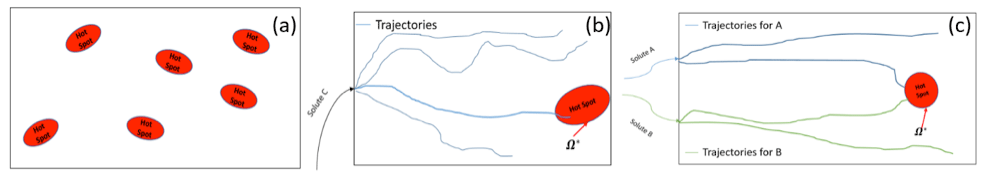
Figure 1 Identified categories of HSHMs. Panel (a) presents HSHMs resulting from a type-A (static) indicator only; panel (b) presents HSHMs resulting from coupled action (static + dynamic), and panel (c) presents HSHMs resulting from multiple (two) dynamic indicators.

2.3 HSHMs induced by type-A (static) and type-B (dynamic) indicators

HSHMs can also result from dynamic processes encountering specific local conditions at Ω^* (Fig. 1b). This is the situation described by Eq. (2), where the type-A indicators are determined first and then used jointly with the type-B indicators for complete HSHM characterization. For example, Bundt et al. (2001) concluded that locations (Ω^*) intersected by preferential flow paths are possible biological hot spots for soil microbial activities. Meanwhile, dynamic factors, such as snowmelt or rainfall infiltration control contaminant transport via the preferential flow paths, thus constitute the hot moment component. Additional case studies are presented in Sect. 3.

For HSHMs induced by both type-A and type-B indicators, the static locations are selected first, based on their HSHM-related properties. After this, we can focus on characterizing the HSHM dynamics as they relate to the relevant locations. A selected location, Ω^*, could become an HSHM site based on characteristics defined through the following type-A and type-B indicators, respectively:

$$\begin{array}{}\text{(4)}& {\displaystyle }& {\displaystyle }{I}_{\mathrm{s}}\left({\mathbf{\Omega }}^{*}\right)=\left\{\begin{array}{cl}\mathrm{1},& \mathrm{if}{Z}_{\mathrm{s}}\left({\mathbf{\Omega }}^{*}\right)\subseteq Z_{\mathrm{s}}^{*}\\ \mathrm{0},& \mathrm{otherwise}\end{array}\right.,\text{(5)}& {\displaystyle }& {\displaystyle }{I}_{\mathrm{d}}\left({\mathbf{\Omega }}^{*},t^{*}\right)=\left\{\begin{array}{cl}\mathrm{1},& \mathrm{if}{Z}_{\mathrm{d}}\left({\mathbf{\Omega }}^{*},t^{*}\right)\subseteq Z_{\mathrm{d}}^{*}\\ \mathrm{0},& \mathrm{otherwise}\end{array}\right.,\text{(6)}& {\displaystyle }& {\displaystyle }{I}_{\mathrm{HSHM}}\left({\mathbf{\Omega }}^{*},t^{*}\right)=\left\{\begin{array}{cl}\mathrm{1},& \mathrm{if}{Z}_{\mathrm{s}}\left({\mathbf{\Omega }}^{*}\right)\subseteq Z_{\mathrm{s}}^{*},\mathrm{and}{Z}_{\mathrm{d}}\left({\mathbf{\Omega }}^{*},t^{*}\right)\subseteq Z_{\mathrm{d}}^{*}\\ \mathrm{0},& \mathrm{otherwise}\end{array}\right.,\end{array}$$

where $Z_{\mathrm{d}}^{*}$ represents the critical conditions needed to trigger the hot moment, whereas $Z_{\mathrm{d}}({\mathbf{\Omega }}^{*},t^{*})$ represents the corresponding, critical-state local conditions at t^* and Ω^*. The statistical model of $I_{\mathrm{HSHM}}({\mathbf{\Omega }}^{*},t^{*})$ can be expressed using the statistical models of I_s and I_d as shown in Eq. (2).

2.4 HSHMs induced by multiple type-B (dynamic) indicators

A confluence of dynamic processes could result in the formation of an HSHM (Fig. 1c). Unlike the previous scenarios where static locations can be determined through known characteristics provided by geophysical or other types of data, HSHMs can also emerge due to a confluence of dynamic processes. For example, Gu et al. (2012) analyzed how streamflow fluctuations could trigger a nitrogen HSHM. In their example, the dynamics of the streamflow and groundwater controlled the transport and mixing of the chemical reactants, thus triggering the occurrences of HSHMs. For this case, the static locations of Ω^* are determined by the confluence of multiple dynamic processes, not being restricted by a set of local conditions. In this case, only type-B indicators need to be modeled.

We can consider the case where an HSHM is predicated on m dynamic processes, d_j, where $I_{\mathrm{d},j}({\mathbf{\Omega }}^{*},t^{*})$ is the dynamic for each dynamic d_j at Ω^* and time t^*. The hotspot location Ω^* is determined by the confluence of all dynamic processes at time t^*. These dynamic processes are not necessarily independent. Therefore, generally, the statistical model for the comprehensive dynamic indicator (which covers all dynamic contributors) assumes the following form:

$$\begin{array}{}\text{(7)}& \begin{array}{rl}P\left[I_{\mathrm{d}}\left({\mathbf{\Omega }}^{*},t^{*}\right)=\mathrm{1}\right]& =P\left[I_{\mathrm{d},\mathrm{1}}\left({\mathbf{\Omega }}^{*},t^{*}\right)\right.\\ & \left.=\mathrm{1},\mathrm{\dots },I_{\mathrm{d},m}\left({\mathbf{\Omega }}^{*},t^{*}\right)=\mathrm{1}\right].\end{array}\end{array}$$

In situations where the various dynamic contributors can be viewed as independent (e.g., Destouni and Cvetkovic, 1991) – i.e., where the reactants travel via different paths – then, assuming independence, we can state that

$$\begin{array}{}\text{(8)}& P\left(I_{\mathrm{d}}\left({\mathbf{\Omega }}^{*},t^{*}\right)=\mathrm{1}\right]=\prod _{j=\mathrm{1}}^{m}P\left[I_{\mathrm{d},j}\left({\mathbf{\Omega }}^{*},t^{*}\right)=\mathrm{1}\right].\end{array}$$

Here, the mean of the dynamic indicator becomes

$$\begin{array}{}\text{(9)}& <I_{\mathrm{d}}\left({\mathbf{\Omega }}^{*},t^{*}\right)\mathit{>=}\prod _{j=\mathrm{1}}^m<I_{\mathrm{d},j}\left({\mathbf{\Omega }}^{*},t^{*}\right)>.\end{array}$$

If Ω^* is a hot spot, then Eq. (9) also defines $<I_{\mathrm{HSHM}}({\mathbf{\Omega }}^{*},t^{*})>$. However, if Ω^* is not a hot spot, then we need to resort to coupled statistical modeling, as suggested by Eq. (2).

2.5 Additional advantages of stochastic formalism

The statistical framework provides several benefits. Unified formulations of HSHMs through indicators provide us with a platform to evaluate alternative HSHM models thoroughly and objectively. For example, the Akaike information criterion (AIC, Akaike, 1974) and Bayesian information criterion (Schwarz, 1978) can be used to rank between alternative indicator formulations and evaluate their ability to explain HSHM observations. Smaller AIC and BIC values indicate more information preserved in a given indicator HSHM model and imply better model quality than other indicator models. On the other hand, if larger AIC and BIC values are observed, important processes for HSHMs are likely missing, indicating the necessity of increasing site characterization and refinement of conceptual models.

In addition, informative priors constructed from similar HSHM sites (Cucchi et al., 2019; Li et al., 2018) could advance early stage planning for HSHM site investigation. Knowledge from studies at similar HSHM sites can be summarized into prior distributions, which can account for variabilities within and between sites. For example, Cucchi et al. (2019) demonstrated how the distribution of hydraulic parameters at unknown target sites can be predicted using information from hydrologically similar sites with existing tool packages such as exPrior. Goal-oriented site characterization also becomes feasible with informative priors; for example, Li et al. (2018) demonstrated the usefulness of informative priors in reducing model uncertainty and potential risks for estimating groundwater drawdown at Mintang tunnel in China. Therefore, through integration with statistical concepts, unified formulations of HSHMs enable us to integrate Bayesian concepts to obtain combined and less risky estimations of HSHMs at new sites, which can help us gain better understanding of the underlying mechanism.

3 Examples of the statistical formulation of HSHMs with case studies

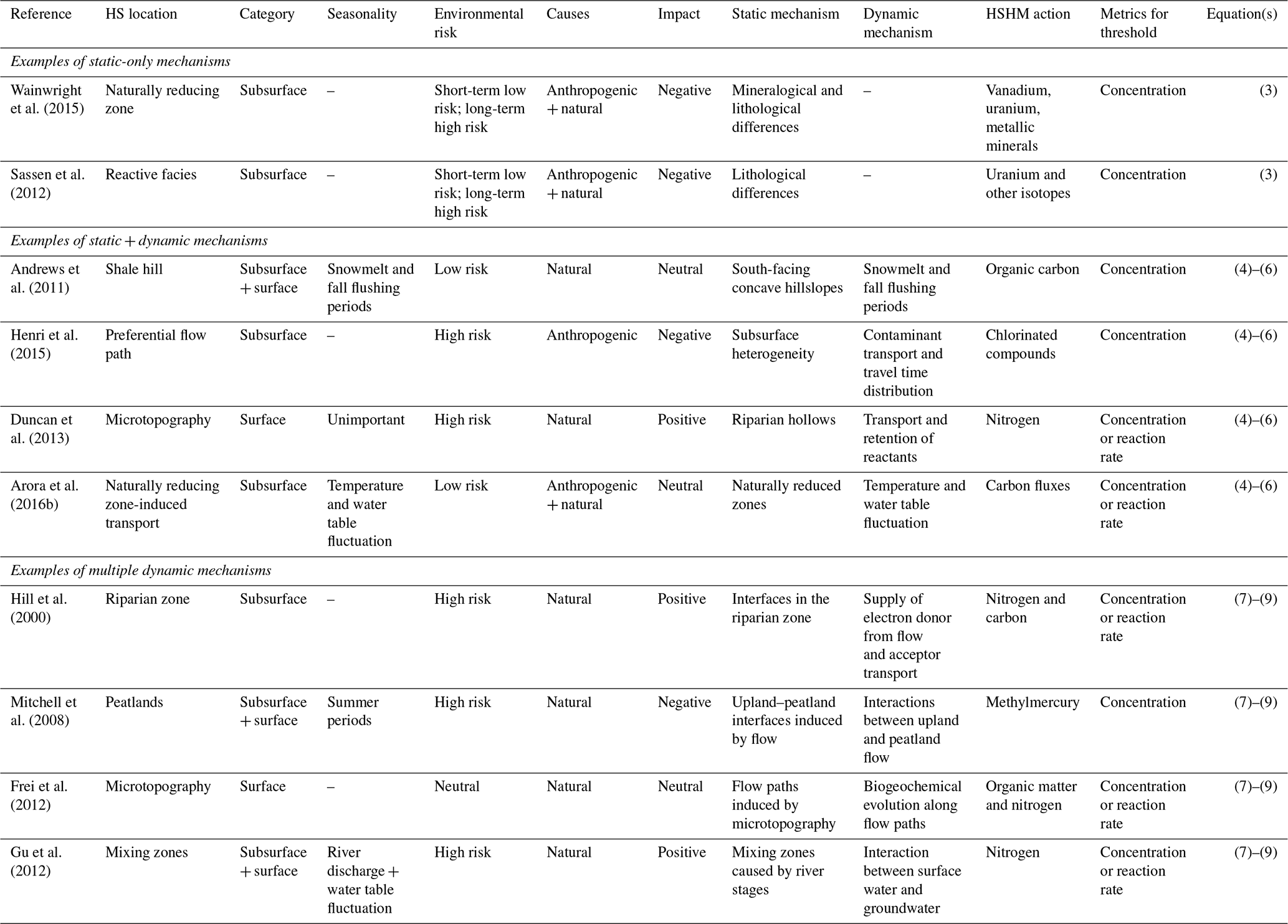
In this section, we selected numerous examples from published research to present how our approach can be used to derive statistical representations for the HSHMs investigated in these studies. We grouped these studies into three categories based on the similarities of their underlying HSHM mechanisms, as described in Sect. 2. Section 3.1 demonstrates the formulation of static-only HSHM; Sect. 3.2 presents the case with static- and dynamic-triggered HSHMs, and Sect. 3.3 summarizes the steps to construct multiple dynamic indicators for HSHMs. Table 1 presents a summary of these cases, where environmental risk levels as well as impacts on the ecosystem were also included.

Table 1 Example cases considered in this study for constructing the statistical formulation of HSHMs.

3.1 HSHMs triggered by static contributors only

In this section, we use Wainwright et al. (2015) as an example to illustrate our process to construct $I_{\mathrm{HSHM}}({\mathbf{\Omega }}^{*},t^{*})$ following Eq. (3), where an HSHM is triggered by static contributors only (Sect. 2.1). NRZs within floodplain environments at the Rifle site are considered biogeochemical hot spots because they represent elevated concentrations of uranium, organic matter, and geochemically reduced minerals, and they have been found to contribute significant carbon fluxes to the atmosphere and to local rivers (Arora et al., 2016a). Due to its characteristics, we considered the spatial distribution of an NRZ to be a static-mechanism-based hot spot. Wainwright et al. (2015) used geophysical data (e.g., induced polarization) to map the distribution of an NRZ at the subsurface level. They found that the phase shift (ϕ) from the induced polarization data of the NRZ was within [4.5, 5] mrad compared to non-NRZ locations at ϕ⊆[1, 3.5] mrad. Thus, ϕ can be used to construct the static indicator with a critical condition of [4.5, 5] mrad. Therefore,

$$\begin{array}{}\text{(10)}& I_{\mathrm{s}}\left({\mathbf{\Omega }}^{*}\right)=\left\{\begin{array}{cl}\mathrm{1},& \mathrm{if}{Z}_{\mathit{\varphi }}\left({\mathbf{\Omega }}^{*}\right)\subseteq [\mathrm{4.5},\mathrm{5}]\mathrm{mrad}\\ \mathrm{0},& \mathrm{otherwise}\end{array}\right..\end{array}$$

Other static attributes, including but not limited to elevation, hydraulic conductivity, and resistivity, can also be used to define the critical conditions to construct the static indicator for hot spots through Bayesian conditioning.

3.2 HSHMs occurring when dynamic contributors coincide at locations defined by static contributors

The second case we present here utilizes Eqs. (4)–(6), where HSHMs are triggered when dynamic contributors coincide at hot spots determined by static contributors. Here, we present the case investigated by Duncan et al. (2013), where riparian hollows representing less than 1 % of the total catchment area contributed more than 99 % of the total denitrification within the watershed. In their study, the denitrification rates peaked during the base flow (midsummer) period, when the riparian hollows were partially oxygenated and the hydrologic fluxes were at a minimum. The site was considered to have low inorganic N availability and, thus, nitrate was supplied via nitrification. The highest rates of denitrification were therefore tied to nitrification and the partially aerated conditions.

The static indicator needs to be constructed based on the micro-topographical features within the riparian zone. Specifically, the topographic wetness index (TWI) (Beven and Kirkby, 1979; Sørensen et al., 2006) was used in Duncan et al. (2013) to delineate the riparian hollows from other riparian locations. Terrain analysis indicated TWI threshold values of 6.0 and 8.0 for riparian hollows under wet and dry conditions, respectively, whereas 4.8 and smaller TWI values corresponded to other riparian locations (e.g., hummocks). Thus, the static indicator can be constructed using the TWI values within the riparian zone to determine the hotspot locations – the hollows. Hence,

$$\begin{array}{}\text{(11)}& \begin{array}{rl}& I_{\mathrm{s}}\left({\mathbf{\Omega }}^{*}\right)=\\ & \left\{\begin{array}{cl}\mathrm{1},& \mathrm{if}{Z}_{\mathrm{TWI}}\left({\mathbf{\Omega }}^{*}\right)>\mathrm{6}\left(\mathrm{wet}\mathrm{condition}\right)\mathrm{or}\mathrm{8}\left(\mathrm{dry}\mathrm{condition}\right)\\ \mathrm{0},& \mathrm{otherwise}\end{array}\right..\end{array}\end{array}$$

Multiple dynamic processes control the denitrification rate at the riparian hollows. As examined by Duncan et al. (2013), a partially aerated condition ($C_{{\mathrm{O}}_{\mathrm{2}}}>\mathrm{5}$ %) is needed to support nitrification, which supplies the nitrate for denitrification. As quiescent, non-storm periods during base flow favor the coupled nitrification–denitrification mechanism, this is another key process that needs to be represented by a dynamic indicator. Although Duncan et al. (2013) did not mention specific concentration ranges for nitrogen species, the major components, such as organic N, should be available. Therefore, we can construct the dynamic indicators as follows:

$$\begin{array}{}\text{(12)}& \begin{array}{rl}P& \left[I_{\mathrm{d}}\left({\mathbf{\Omega }}^{*},t^{*}\right)=\mathrm{1}\right]=P\left[I_{\mathrm{d},{\mathrm{O}}_{\mathrm{2}}}\left({\mathbf{\Omega }}^{*},t^{*}\right)\right.\\ & \left.=\mathrm{1},I_{\mathrm{d},\mathrm{Hydro}}\left({\mathbf{\Omega }}^{*},t^{*}\right)=\mathrm{1},I_{\mathrm{d},\mathrm{N}}\left({\mathbf{\Omega }}^{*},t^{*}\right)=\mathrm{1}\right],\end{array}\end{array}$$

where $I_{\mathrm{d},\mathrm{Hydro}}({\mathbf{\Omega }}^{*},t^{*})$ is the dynamic indicator representing the streamflow stages; this will be 1 if the base flow conditions are met. Additionally, here, $I_{\mathrm{d},\mathrm{N}}({\mathbf{\Omega }}^{*},t^{*})$ is the dynamic indicator for the transport of the nitrogen species in the subsurface that support the coupled nitrification–denitrification mechanism.

$$\begin{array}{}\text{(13)}& {\displaystyle }& {\displaystyle }{I}_{\mathrm{d},{\mathrm{O}}_{\mathrm{2}}}\left({\mathbf{\Omega }}^{*},t^{*}\right)=\left\{\begin{array}{cl}\mathrm{1},& \mathrm{if}{C}_{{\mathrm{O}}_{\mathrm{2}}}\left({\mathbf{\Omega }}^{*},t^{*}\right)>\mathrm{5}\mathit{\%}\\ \mathrm{0},& \mathrm{otherwise}\end{array}\right.,\text{(14)}& {\displaystyle }& {\displaystyle }{I}_{\mathrm{d},\mathrm{Hydro}}\left({\mathbf{\Omega }}^{*},t^{*}\right)=\left\{\begin{array}{cl}\mathrm{1},& \mathrm{if}{t}^{*}\subseteq \mathrm{base}\mathrm{flow}\mathrm{periods}\\ \mathrm{0},& \mathrm{otherwise}\end{array}\right.,\text{(15)}& {\displaystyle }& {\displaystyle }{I}_{\mathrm{d},\mathrm{N}}\left({\mathbf{\Omega }}^{*},t^{*}\right)=\left\{\begin{array}{cl}\mathrm{1},& \mathrm{if}{C}_{\mathrm{N}}\left({\mathbf{\Omega }}^{*},t^{*}\right)>\mathrm{0}\\ \mathrm{0},& \mathrm{otherwise}\end{array}\right.\end{array}$$

It is noted that these dynamic processes are not statistically independent. Usually, when one condition is met (e.g., base flow conditions), other conditions may consistently be satisfied (e.g., the transport of nitrogen in riparian hollows). Alternatively, numerical modeling approaches can be used to construct the dynamic indicators based on the critical conditions at riparian hollows (Ω^*), where we could directly target N₂ fluxes using a Monte Carlo approach. The statistical formulation used here is constructed specifically for the mechanisms described by Duncan et al. (2013). Thus, the detailed threshold limits could change under other denitrification HSHM cases, such as the case presented in Hill et al. (2000), who focus on desert landscapes, or the one by Harms and Grimm (2008), where the monsoon season is influential for the nitrogen transport. Nonetheless, the general formulation of HSHMs using indicators is still applicable.

3.3 HSHMs occurring when multiple dynamic processes converge in space

HSHMs can also be triggered by the confluence of multiple dynamic processes that lead to the convergence of complementary reactants at Ω^*. Complementary reactants can be mobilized and transported via different hydrologic flow paths. They can converge at hotspot locations and trigger hot moments during the mixing. Following the statistical framework developed in this study, Eqs. (7) to (9) are suitable for this condition. In order to illustrate how the dynamic indicators are constructed, we consider here the case reported by Gu et al. (2012), where high biogeochemical activity was observed at the interface of groundwater and surface water during the stream stage fluctuations, which resulted in significant in-stream denitrification and ${\mathrm{NO}}_{\mathrm{3}}^{-}$ removal.

In their study, hot spots form around the near-stream riparian subsurface during river stage fluctuations, where active biogeochemical reaction (e.g., denitrification) requires both O₂ depletion and the simultaneous presence of ${\mathrm{NO}}_{\mathrm{3}}^{-}$ and the dissolved organic carbon (DOC). Specifically, the spatiotemporal distribution of denitrification hot spots coincides with an O₂ depletion zone along the DOC infiltration flow paths. In order to determine the mixing of groundwater and surface water during stage fluctuations, Gu et al. (2012) defined bank storage volume V(t) and maximum bank storage volume V_max. The flood hydrograph was subdivided into the rising limbs, recession limbs and return flow, the latter representing the slow restitution of part of the water that infiltrated during the previous stages. Considering the different dynamics of these components, they observed that the largest infiltration rate occurred prior to the maximum stage rise, while V_max=5 m³ m⁻¹ (critical condition) occurred in the recession limb of the flood event. Instead, maximum return flow occurred toward the end of the recession curve before the stream hydrograph stabilizes. Maximum ${\mathrm{NO}}_{\mathrm{3}}^{-}$ rate removal occurred when the return flow phase was almost complete and then decreased until the depletion of ${\mathrm{NO}}_{\mathrm{3}}^{-}$. Through statistical analysis, they found that V_max, viewed as an integrated index for hydrological exchange, could explain 64 % of the variation in the ${\mathrm{NO}}_{\mathrm{3}}^{-}$ removal. Thus, V_max can be used as the critical state to determine whether or not the hyporheic dynamics is significant to enhance relevant biogeochemical processes. In order for the hot moments to be significant, the stream–riparian zone should also be microbially active. Based on these conditions, the dynamic indicators can be constructed as follows:

$$\begin{array}{}\text{(16)}& \begin{array}{rl}P\left[I_{\mathrm{d}}\left({\mathbf{\Omega }}^{*},t^{*}\right)=\mathrm{1}\right]=& P\left[I_{\mathrm{d},\mathrm{Hydro}}\left({\mathbf{\Omega }}^{*},t^{*}\right)=\mathrm{1},\right.\\ & \left.I_{\mathrm{d},\mathrm{Chem}}\left({\mathbf{\Omega }}^{*},t^{*}\right)=\mathrm{1}\right],\end{array}\end{array}$$

where $I_{\mathrm{d},\mathrm{Hydro}}({\mathbf{\Omega }}^{*},t^{*})$ represents the dynamic process induced by the hydrologic conditions (e.g., stage fluctuation), and $I_{\mathrm{d},\mathrm{Chem}}({\mathbf{\Omega }}^{*},t^{*})$ represents the dynamic process controlled by the transport and accumulation of chemical reactants. Based on the critical values or ranges, we formulate the indicators as follows:

$$\begin{array}{}\text{(17)}& \begin{array}{rl}& I_{\mathrm{d},\mathrm{Hydro}}\left({\mathbf{\Omega }}^{*},t^{*}\right)=\left\{\begin{array}{cl}\mathrm{1},& Z_{V_{\max }}\left({\mathbf{\Omega }}^{*},t^{*}\right)\ge \mathrm{5}{\mathrm{m}}^{\mathrm{3}}{\mathrm{m}}^{-\mathrm{1}}\\ \mathrm{0},& \mathrm{otherwise}\end{array}\right.,\\ & I_{\mathrm{d},\mathrm{Chem}}\left({\mathbf{\Omega }}^{*},t^{*}\right)=\left\{\begin{array}{cl}\mathrm{1},& \mathrm{if}{C}_{{\mathrm{O}}_{\mathrm{2}}}\left({\mathbf{\Omega }}^{*},t^{*}\right)\mathrm{is}\mathrm{small}\mathrm{and}{C}_{{\mathrm{NO}}_{\mathrm{3}}^{-}}\\ & \left({\mathbf{\Omega }}^{*},t^{*}\right)>\mathrm{0}\mathrm{and}{C}_{\mathrm{DOC}}\left({\mathbf{\Omega }}^{*},t^{*}\right)>\mathrm{0}\\ \mathrm{0},& \mathrm{otherwise}\end{array}\right..\end{array}\end{array}$$

Typically, because of the complexity of the processes, no analytical solutions are available for formulating the indicators. However, Monte Carlo simulations can be useful in constructing such indicators. For this case, an HSHM at any given location and tim (${\mathbf{\Omega }}^{*},t^{*}$) will only be triggered when all of the conditions are met and the ensemble mean of the indicator assumes the following form:

$$\begin{array}{}\text{(18)}& <I_{\mathrm{d}}\left({\mathbf{\Omega }}^{*},t^{*}\right)\mathit{>=}{\displaystyle \frac{\mathrm{1}}{N}}\sum _{i=\mathrm{1}}^N{I}_{\mathrm{d},i}\left({\mathbf{\Omega }}^{*},t^{*}\right),\end{array}$$

where $I_{\mathrm{d},i}({\mathbf{\Omega }}^{*},t^{*})$ is the value that the indicator assumes in the ith realization and N is the total number of realizations.

Overall, our choices of the three studies should not limit the generalizability of the indicator statistics approach for deriving statistical formulations for HSHM applications. The critical conditions chosen to construct the indicators are determined solely on the findings from these selected studies, and they will vary under different scenarios.

4 HSHM applications in groundwater hydrology

This section focuses on HSHMs in the subsurface for demonstration of linking HSHM models with the contributing physical processes, such as the migration of groundwater carrying reducing substrates, nuclear waste transport within the subsurface, the accumulation and transport of dense non-aqueous phase liquid (DNAPL) and other biogeochemical processes. Some current modeling approaches that focus on subsurface HSHMs assume simplified hydrologic structures (e.g., homogeneous and isotropic domains) in quantifying the fate and transport of solutes in the subsurface. However, such assumptions neglect the effect of the heterogeneity in the subsurface, potentially missing localized HSHMs arising as the combined effect of heterogeneity in physical and geochemical properties, and do not allow us to assess uncertainties in the HSHM occurrences.

This section therefore focuses on HSHMs taking place in the subsurface, with a particular emphasis on the role of spatial variability of the hydrologic parameters. Section 4.1 illustrates the potential of subsurface heterogeneity for triggering and timing of HSHMs. In Sect. 4.2, we develop closed-form analytical solutions for HSHM probability. In doing this, we demonstrate the linking between our indicator model and the physics of the HSHMs in the subsurface. In Sect. 4.3 we demonstrate applications under various conditions of spatial variability.

4.1 Importance of spatial variability in the subsurface

The heterogeneous structure of hydraulic conductivity leads to significant variability in the transport of solutes in the subsurface, which couples with heterogeneous geochemical properties leading to a spatially varying reactivity (Arora et al., 2019b; Loschko et al., 2016; Sassen et al., 2012; Wainwright et al., 2015). Figure 2 demonstrates the uncertainty associated with HSHMs by looking at the flow fields in two-dimensional log-hydraulic conductivity (Y=ln (K)) fields with streamlines resulting from a uniform mean head gradient, left to right. The three panels differ in terms of the variance, ${\mathit{\sigma }}_Y^{\mathrm{2}}$, of the log conductivity. The covariance function used for generating the fields is exponential and isotropic. ${\mathit{\sigma }}_Y^{\mathrm{2}}$ is shown to have a profound impact upon the conductivity field. As the variance increases, regions of high and low log conductivity emerge, creating preferential flow paths bypassing the low-conductivity zones as shown by particle trajectories. At smaller variance (i.e., ${\mathit{\sigma }}_Y^{\mathrm{2}}=\mathrm{0.1}$), particles mainly travel along the mean flow direction with very limited departure from the mean trajectory, which are the straight lines connecting the left and right boundaries. In this situation, the arrival times of solute particles at a critical location (i.e., Ω^*, where for example geochemical conditions are favorable for certain types of reactions to occur) are predictable. With large variances (i.e., ${\mathit{\sigma }}_Y^{\mathrm{2}}=\mathrm{2}$), the streamlines assume a very irregular, hard-to-predict geometry, and we can observe the emergence of flow channels, where particles can move quickly next to stagnant flow regions. Arrival times become more uncertain, because the exact geometry of the streamlines is hard to predict unless the Y field is known deterministically. However, since this is never the case, in another equally likely realization of the Y field, the situation may be different, resulting in significant uncertainties in predicting the particle travel times. Thus, spatial variability of log conductivity is a major uncertainty-inducing factor and, by extension, requires the need for stochastic modeling of HSHMs in situations where the associated processes and attributes are subject to uncertainty. In the following sections, we will present illustrative examples to analyze how subsurface spatial variability influences $<I_{\mathrm{HSHM}}({\mathbf{\Omega }}^{*},t^{*})>$, including variance and anisotropy ratio of the log conductivity.

Figure 2 Illustrative example of a heterogeneous log-hydraulic conductivity field and solute particle transport. Black lines represent simulated particle travel paths. A left to right hydraulic gradient of 0.1 is applied. Mean of log conductivity is set at −3. Note that color scales for log conductivity are consistent in all three panels.

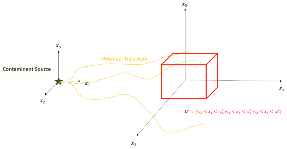
Figure 3 Configuration of the synthetic case study. x₁, x₂ and x₃ represent the longitudinal, transverse and vertical directions, respectively. w₁, $w_{\mathrm{1}}^{\prime }$, w₂, $w_{\mathrm{2}}^{\prime }$, w₃ and $w_{\mathrm{3}}^{\prime }$ are the coordinates that set up the volume of Ω^*.

4.2 Illustrative example and indicator formulation

In this section we illustrate the proposed indicator approach by means of synthetic case studies developed by using methods of stochastic hydrogeology. The choice of the synthetic case studies does not limit our approaches to broader applications where stochastic modeling with Monte Carlo simulations is applicable. Figure 3 displays the configuration of this case example. Consider the case of an instantaneous point source release of a target compound at location x₀ and time t₀. HSHMs are triggered at any (${\mathbf{\Omega }}^{*},t^{*}$) if the solute is present. Consider the hot spot (Ω^*) to be confined within the following volume: $w_{\mathrm{1}}\le x_{\mathrm{1}}\le w_{\mathrm{1}}^{\prime }$; $w_{\mathrm{2}}\le x_{\mathrm{2}}\le w_{\mathrm{2}}^{\prime }$; $w_{\mathrm{3}}\le x_{\mathrm{3}}\le w_{\mathrm{3}}^{\prime }$; the dynamic indicator is therefore defined as follows:

$$\begin{array}{}\text{(19)}& I_{\mathrm{d}}\left({\mathbf{\Omega }}^{*},t^{*}\right)=\left\{\begin{array}{cl}\mathrm{1},& \mathrm{if}X\left(t^{*}\right)\subseteq {\mathbf{\Omega }}^{*}\mathrm{at}{t}^{*}\\ \mathrm{0},& \mathrm{otherwise}\end{array}\right..\end{array}$$

The injected solute can be modeled in a Lagrangian framework as a particle moving according to the velocity field without changing its volume. The latter is the consequence of neglecting pore-scale dispersion. The expected value of this dynamic indicator at t^* is therefore

$$\begin{array}{}\text{(20)}& <I_{\mathrm{d}}\left({\mathbf{\Omega }}^{*},t^{*}\right)\mathit{>=}\underset{\mathrm{\Omega }}{\overset{*}{\int }}{f}_{\mathbf{X}\left({\mathit{t}}^{*}\right)}\left(\mathit{a}\mathrm{|}{\mathit{x}}_{\mathrm{0}},t_{\mathrm{0}}\right)d\mathit{a},\end{array}$$

where $f_{\mathbf{X}\left({\mathit{t}}^{*}t\right)}(\mathit{a}\mathrm{|}{\mathit{x}}_{\mathrm{0}},t_{\mathrm{0}})$ is the probability distribution function (pdf) of the particle's trajectory at time t^* (Dagan and Nguyen, 1989; Rubin, 2003). If we also assume steady, uniform in the average flow with mild heterogeneity of the log hydraulic conductivity field with the Gaussian displacement pdf, then we can compute $<I_{\mathrm{HSHM}}\left({\mathbf{\Omega }}^{*}{t}^{*}\right)>$ analytically using the following equation:

$$\begin{array}{}\text{(21)}& \begin{array}{rl}P& \left(I_{\mathrm{HSHM}}\left({\mathbf{\Omega }}^{*},t^{*}\right)=\mathrm{1}\right)=<I_{\mathrm{HSHM}}\left({\mathbf{\Omega }}^{*},t^{*}\right)>\\ & =<I_{\mathrm{s}}\left({\mathbf{\Omega }}^{*}\right)><\left(I_{\mathrm{d}}\left({\mathbf{\Omega }}^{*},t^{*}\right)\right)>\\ & =\mathrm{prob}\left(I_{\mathrm{d}}\left({\mathbf{\Omega }}^{*},t^{*}\right)=\mathrm{1}\right)=\mathrm{prob}\left\{X\left(t^{*}\right)\subseteq {\mathbf{\Omega }}^{*}\right\}\\ & =\prod _{i=\mathrm{1}}^m\underset{w_i}{\overset{w_i^{\prime }}{\int }}{f}_{X_i\left(t^{*}\right)}\left(a_i\mathrm{|}{x}_{\mathrm{0}},t_{\mathrm{0}}\right)d{a}_i=\underset{w_{\mathrm{1}}}{\overset{w_{\mathrm{1}}^{\prime }}{\int }}{f}_{X_{\mathrm{1}}\left(t^{*}\right)}\left(a_{\mathrm{1}}\mathrm{|}{x}_{\mathrm{0}},t_{\mathrm{0}}\right)d{a}_{\mathrm{1}}\\ & \underset{w_{\mathrm{2}}}{\overset{w_{\mathrm{2}}^{\prime }}{\int }}{f}_{X_{\mathrm{2}}\left(t^{*}\right)}\left(a_{\mathrm{2}}\mathrm{|}{x}_{\mathrm{0}},t_{\mathrm{0}}\right)d{a}_{\mathrm{2}}\underset{w_{\mathrm{3}}}{\overset{w_{\mathrm{3}}^{\prime }}{\int }}{f}_{X_{\mathrm{3}}\left(t^{*}\right)}\left(a_{\mathrm{3}}\mathrm{|}{x}_{\mathrm{0}},t_{\mathrm{0}}\right)d{a}_{\mathrm{3}}\\ & ={\displaystyle \frac{\mathrm{1}}{(\mathrm{2}\mathit{\pi }{)}^{\frac{\mathrm{3}}{\mathrm{2}}}\sqrt{X_{\mathrm{11}}\left(t^{*}\right)X_{\mathrm{22}}\left(t^{*}\right)X_{\mathrm{33}}\left(t^{*}\right)}}}\underset{w_{\mathrm{1}}}{\overset{w_{\mathrm{1}}^{\prime }}{\int }}\\ & \exp \left[-{\displaystyle \frac{\mathrm{1}}{\mathrm{2}}}{\displaystyle \frac{{\left(a_{\mathrm{1}}-U{t}^{*}\right)}^{\mathrm{2}}}{X_{\mathrm{11}}\left(t^{*}\right)}}\right]d{a}_{\mathrm{1}}\cdot \underset{w_{\mathrm{2}}}{\overset{w_{\mathrm{2}}^{\prime }}{\int }}\exp \left[-{\displaystyle \frac{\mathrm{1}}{\mathrm{2}}}{\displaystyle \frac{a_{\mathrm{2}}^{\mathrm{2}}}{X_{\mathrm{22}}\left(t^{*}\right)}}\right]\\ & d{a}_{\mathrm{2}}\underset{w_{\mathrm{3}}}{\overset{w_{\mathrm{3}}^{\prime }}{\int }}\exp \left[-{\displaystyle \frac{\mathrm{1}}{\mathrm{2}}}{\displaystyle \frac{a_{\mathrm{3}}^{\mathrm{2}}}{X_{\mathrm{33}}\left(t^{*}\right)}}\right]d{a}_{\mathrm{3}},\end{array}\end{array}$$

which can be integrated to yield

$$\begin{array}{}\text{(22)}& \begin{array}{rl}P& \left(I_{\mathrm{HSHM}}\left({\mathbf{\Omega }}^{*},t^{*}\right)=\mathrm{1}\right)=<I_{\mathrm{HSHM}}\left({\mathbf{\Omega }}^{*},t^{*}\right)>\\ & ={\displaystyle \frac{\mathrm{1}}{\mathrm{8}}}\left[\mathrm{erfc}\left({\displaystyle \frac{w_{\mathrm{1}}-U{t}^{*}}{\sqrt{\mathrm{2}{X}_{\mathrm{11}}\left(t^{*}\right)}}}\right)-\mathrm{erfc}\left({\displaystyle \frac{w_{\mathrm{1}}^{\prime }-U{t}^{*}}{\sqrt{\mathrm{2}{X}_{\mathrm{11}}\left(t^{*}\right)}}}\right)\right]\\ & \cdot \left[\mathrm{erfc}\left({\displaystyle \frac{w_{\mathrm{2}}}{\sqrt{\mathrm{2}{X}_{\mathrm{22}}\left(t^{*}\right)}}}\right)-\mathrm{erfc}\left({\displaystyle \frac{w_{\mathrm{2}}^{\prime }}{\sqrt{\mathrm{2}{X}_{\mathrm{22}}\left(t^{*}\right)}}}\right)\right]\\ & \left[\mathrm{erfc}\left({\displaystyle \frac{w_{\mathrm{3}}}{\sqrt{\mathrm{2}{X}_{\mathrm{33}}\left(t^{*}\right)}}}\right)-\mathrm{erfc}\left({\displaystyle \frac{w_{\mathrm{3}}^{\prime }}{\sqrt{\mathrm{2}{X}_{\mathrm{33}}\left(t^{*}\right)}}}\right)\right].\end{array}\end{array}$$

For simplicity, but without lack of generality, in Eq. (20) we assumed ${\mathit{x}}_{\mathrm{0}}=(\mathrm{0},\mathrm{0},\mathrm{0})$. The displacement variances X_ii, i=1, 2, 3 depend on the spatial distribution of the hydraulic conductivity in the subsurface. Equations (A4) to (A6) present the displacement variances for an axisymmetric exponential covariance function of the log conductivity (Eq. A3) given in Appendix A. In Eqs. (A7) to (A19), we have provided derivations of indicator formulations for other HSHM scenarios, including indicator formulation for complex concentration thresholds and indicator formulation for hot moment durations. Notice that in obtaining Eq. (20) we postulated ergodicity, which in practical terms reflects the actual situation of an instantaneous injection into a source zone with a transverse dimension much larger than the integral scale of the hydraulic conductivity (Dagan, 1990), such that the ensemble mean is representative of the effects of the actual, but unknown, distribution of hydraulic conductivity.

4.3 Probability of HSHM occurrence controlled by subsurface heterogeneity

In the following sections, we present the results from the case study described in Sect. 4.2. Specifically, in Sect. 4.3.1 and 4.3.2, we explore how heterogeneity of log-hydraulic conductivity influences the probability of HSHM occurrences. To make results as general as possible, lengths are made dimensionless with respect to the integral scales ($I_{Y_{\mathrm{h}}}$ in the two horizontal directions and $I_{Y_{\mathrm{v}}}$ in the vertical one) and time with respect to the following advective timescale: $I_{Y_{\mathrm{h}}}/U$, where U is the mean velocity. In the following, we explore the effect of the remaining parameters, i.e., the anisotropy ratio $e=\frac{I_{Y_{\mathrm{V}}}}{I_{Y_{\mathrm{H}}}}$ and the variance of the log conductivity ${\mathit{\sigma }}_Y^{\mathrm{2}}$, on the emergence of an HSHM. We placed Ω^* along the mean trajectory at ($\mathrm{21}{I}_{Y_{\mathrm{H}}}$, 0, 0) with dimensions as ($\mathrm{2}{I}_{Y_{\mathrm{H}}}$, $\mathrm{2}{I}_{Y_{\mathrm{H}}}$, $\mathrm{2}{I}_{Y_{\mathrm{V}}}$). The dimensions of the hot spot are therefore of two integral scales in the three coordinate directions (x₁, x₂, x₃) and are placed at a dimensionless distance of 21 from the point source.

4.3.1 Dependence of $P\left(I_{\mathrm{HSHM}}\right({\mathrm{\Omega }}^{*},\mathit{\tau })=\mathrm{1})$ on variance in the spatial correlation structure of the log conductivity

Figure 4 shows $P\left(I_{\mathrm{HSHM}}\right({\mathbf{\Omega }}^{*},\mathit{\tau })=\mathrm{1})$, which is the probability that an HSHM is triggered at Ω^* and the dimensionless time $\mathit{\tau }=\frac{tU}{I_{Y_{\mathrm{h}}}}$, for a few values of ${\mathit{\sigma }}_Y^{\mathrm{2}}$. Here, $I_{\mathrm{HSHM}}({\mathbf{\Omega }}^{*},\mathit{\tau })=\mathrm{1}$ represents the situation in which an HSHM is triggered. At early time (e.g., τ<5), larger probability $P\left(I_{\mathrm{HSHM}}\right({\mathbf{\Omega }}^{*},\mathit{\tau })=\mathrm{1})$ is observed with increase in ${\mathit{\sigma }}_Y^{\mathrm{2}}$. At intermediate time, i.e., at times comparable with the mean travel time τ=21, $P\left(I_{\mathrm{HSHM}}\right({\mathbf{\Omega }}^{*},\mathit{\tau })=\mathrm{1})$ is inversely proportional to ${\mathit{\sigma }}_Y^{\mathrm{2}}$. At late time (e.g., τ>40), the largest $P\left(I_{\mathrm{HSHM}}\right({\mathbf{\Omega }}^{*},\mathit{\tau })=\mathrm{1})$ occurs at intermediate ${\mathit{\sigma }}_Y^{\mathrm{2}}$. We observe that ${\mathit{\sigma }}_Y^{\mathrm{2}}$ regulates the timing of the peak in $P\left(I_{\mathrm{HSHM}}\right({\mathbf{\Omega }}^{*},\mathit{\tau })=\mathrm{1})$, which is located in the proximity of the mean travel time, τ=21, for weak heterogeneity and shifts towards earlier times as ${\mathit{\sigma }}_Y^{\mathrm{2}}$ increases. From the practical perspective, Fig. 4 shows the probability of developing an HSHM at the identified position Ω^* at the given time τ.

Figure 4 Dependence of $P\left(I_{\mathrm{HSHM}}\right({\mathrm{\Omega }}^{*},\mathit{\tau })=\mathrm{1})$ on time (τ) and on the level of spatial variability of the log-hydraulic conductivity (${\mathit{\sigma }}_Y^{\mathrm{2}}$).

These effects relate to the relationship between travel times (from the source to Ω^*) and ${\mathit{\sigma }}_Y^{\mathrm{2}}$. The key point to note is that ${\mathit{\sigma }}_Y^{\mathrm{2}}$ controls the spread of the travel time around its mean value. A larger ${\mathit{\sigma }}_Y^{\mathrm{2}}$ enhances channeling effects (Fiori and Jankovic, 2012; Moreno and Tsang, 1994, also in Fig. 2), which in turn enable earlier arrival times. However, at the same time, it also leads to the emergence of low-conductivity zones with low velocity or stagnant groundwater. The solute tends to bypass low hydraulic conductivity zones, as shown by the streamlines depicted in Fig. 2; however, the small amount of solute that actually penetrates these zones by slow advection and diffusion gets trapped for long time before being released, and this results in an extended tailing with low concentration, which increases the probability of observing an HSHM at later times. Thus, with an increase in ${\mathit{\sigma }}_Y^{\mathrm{2}}$, we notice an increase in the probability of observing both increasingly earlier and increasingly delayed arrival times, which widens the probability distribution. By contrast at small variance, particles deviate little from the ensemble mean trajectory, because of the small contrast in conductivity between high- and low-conductivity zones. This results in small particle spreading and travel times that differ only slightly from the mean travel time (τ=21) and a probability distribution less spread around the mean, where the peak is observed.

In summary, hydraulic conductivity contrast between low- and high-conductivity lithofacies increases with ${\mathit{\sigma }}_Y^{\mathrm{2}}$, leading to the emergence of organized high-conductivity pathways sneaking through surrounding low-conductivity zones, with the latter acting as “trapping” elements. This causes the emergence of both early and late arrival times, with the consequent larger probability of triggering HSHMs at early and later times, with respect to the case of low heterogeneity. Early arrival times are controlled by the connected high-conductivity pathways, and the late arrival times are influenced by the low-conductivity zones, which act as low-release reservoirs for solutes.

4.3.2 Dependence of $P\left(I_{\mathrm{HSHM}}\right({\mathbf{\Omega }}^{*},\mathit{\tau })=\mathrm{1})$ on anisotropy in the spatial correlation structure of the log-hydraulic conductivity

The discussion here (accompanying Fig. 5) focuses on the impact of the anisotropy ratio in the correlation structure (e, defined above) on the probability of triggering HSHMs. The anisotropy ratio, e, provides an indication of the persistence of the log conductivity (Y) in the principal directions. The spatial correlation model used here for demonstration is that of axis symmetry, which is common to sedimentary formations (Dagan, 1989; Rubin, 2003), with e providing the ratio between the persistence of Y in the vertical (x₃) direction, represented by $I_{Y_{\mathrm{V}}}$, and the ones on the horizontal plane (x₁–x₂), represented by $I_{Y_{\mathrm{H}}}$. In unconsolidated sedimentary formations, $I_{Y_{\mathrm{V}}}$ is typically smaller than $I_{Y_{\mathrm{H}}}$ by as much as 1 order of magnitude, due to the different timescales of the depositional process taking place in the horizontal and vertical directions, which leads to thin and elongated lithofacies and consequently to a much smaller persistence of Y values in the normal to horizontal plane (Miall, 1985, 1988; Ritzi et al., 2004).

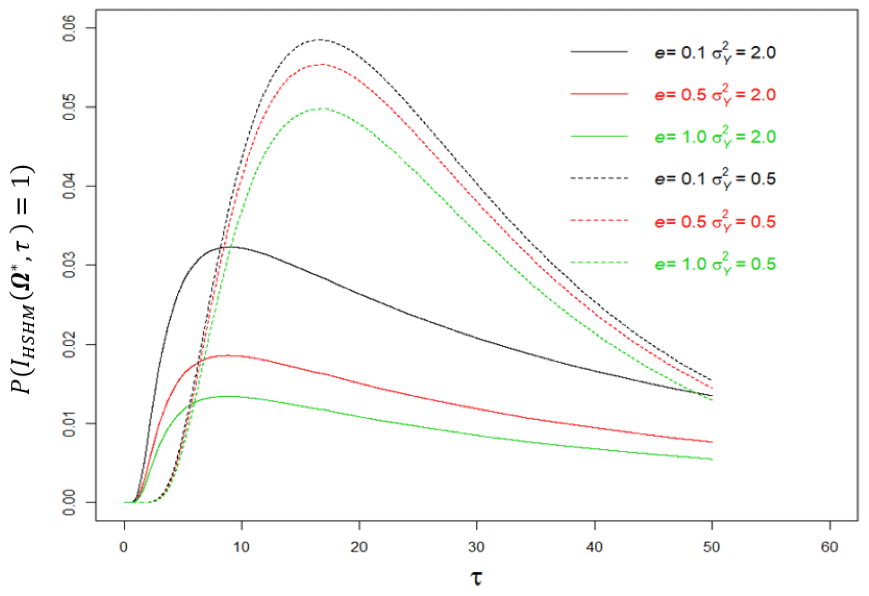
Figure 5 Dependence of $P\left(I_{\mathrm{HSHM}}\right({\mathrm{\Omega }}^{*},\mathit{\tau })=\mathrm{1})$ on (τ) and on anisotropy ratio e. Solid and dashed lines represent, respectively, the probabilities of large (${\mathit{\sigma }}_Y^{\mathrm{2}}=\mathrm{2.0}$) and small (${\mathit{\sigma }}_Y^{\mathrm{2}}=\mathrm{0.5}$) variance of the log-hydraulic conductivity.

Figure 5 compares $P\left(I_{\mathrm{HSHM}}\right({\mathbf{\Omega }}^{*},\mathit{\tau })=\mathrm{1})$ between formations defined by different anisotropy ratios and different ${\mathit{\sigma }}_Y^{\mathrm{2}}$. It shows that we have two factors to consider when explaining the differences in $P\left(I_{\mathrm{HSHM}}\right({\mathbf{\Omega }}^{*},\mathit{\tau })=\mathrm{1})$. The first factor, as discussed earlier, is the widening of the probability distribution (direct consequence of the widening of the travel time distribution) due to increase in ${\mathit{\sigma }}_Y^{\mathrm{2}}$. With larger variance, we observe higher probabilities of departure of the travel times away from the average. The anisotropy ratio e adds a compounding factor. To understand its effect, we should recall the analyses of lateral displacement variances of solute particles moving in heterogeneous formations (cf. Dagan, 1989, and Eqs. A4 to A6 here), showing that smaller e leads to smaller lateral (both vertical and horizontal) displacement variances, implying smaller probabilities of lateral departures from the mean flow trajectory. Smaller e limits lateral spreads and increases the probability of particles entering Ω^*, sooner or later, and triggering HSHMs. The effect could also be viewed as a channeling effect of sorts: smaller e implies Y blocks of small aspect ratio (i.e., long but thin elements), which provide fast tracks for particles when defined by high Y values while blocking lateral spreads when defined by low Y values.

Additional notes: first, Ω^* known in the present analysis is located downstream from the source, along with the mean trajectory of the solute displacement. We expect different results in situations where Ω^* is positioned at an offset with respect to the mean flow direction or when its position is unknown. In both cases we expect a reduction of the probability of triggering an HSHM. Relevant to our discussion is that the proposed probabilistic framework can address the case of an unknown position for Ω^* as well. Second, we note that the analytical models used to compute the displacement statistics are formally limited to small variance of the log conductivity (${\mathit{\sigma }}_Y^{\mathrm{2}}<\mathrm{1}$), although they are shown to provide good approximations for large variances (Bellin et al., 1992; Salandin and Fiorotto, 1998). Third, the stochastic formulation provides the theoretical and computational formalism for conditioning the probabilities on in situ measurements (Ezzedine and Rubin, 1996; Rubin and Dagan, 1992) as well as on information borrowed from similar sites (Li et al., 2018; Cucchi et al., 2019).

5 Discussion and summary

In this study, we developed a general stochastic framework for characterizing the spatiotemporal distribution of environmental hot spots and hot moments (HSHMs). The stochastic formulation is built around the following principles.

• The HSHMs are defined as random variables, and the goal is to derive their stochastic distribution in terms of the relevant processes and attributes.

• The processes and attributes are modeled as stochastic processes and random variables, respectively, based on the underlying physics.

• The static contributors are modeled stochastically using geostatistical space random functions.

• The dynamic contributors are modeled stochastically using probability distribution functions derived from the underlying mathematical–physical models.

• Several HSHM categories are defined, based on the contributing factors, as follows: HSHMs defined by dynamic contributors only, HSHMs defined by static contributors, and, most commonly, HSHMs requiring the coupling of static and dynamic contributors. The HSHM stochastic formulations are expressed in terms of the stochastic formulations of the relevant contributors.

We provided a detailed review of multiple HSHMs and showed how they relate to our definitions.

The framework we proposed in this study is advantageous in that it allows us to calculate the uncertainty associated with HSHMs based on the uncertainty associated with its contributors. Additionally, it provides a formalism, well established by Bayesian theory, for conditioning the HSHM probabilities on in situ measurements as well as on information borrowed from geologically and otherwise similar sites.

We demonstrated our proposed approach through applications in the area of subsurface transport and hydrogeology, focusing on the impacts of subsurface heterogeneity on HSHMs. We analyzed, quantitatively, how subsurface heterogeneity of the conductivity field controls the HSHM statistics, for example, the time expected for the probability of the HSHM to occur to reach a priori set thresholds or time to peak probability.

Lastly, as mentioned both here and in previous studies, statistical methods for quantifying the occurrences of HSHMs and the associated uncertainties are needed to advance our understanding of the mechanisms that cause HSHMs, as well as to enhance our ability to predict HSHMs and manage their consequences.

Appendix A: Equations and derivations

A1 Equations for the displacement pdf

Assuming steady uniformity in the average flow, with mild heterogeneity of the log-hydraulic conductivity field with Gaussian displacement, the pdf of the longitudinal (x₁, Fig. 3) displacement of a solute particle starting at time t₀=0 at ${\mathit{x}}_{\mathrm{0}}=(\mathrm{0},\mathrm{0},\mathrm{0})$ is given by the following equation (Dagan and Nguyen, 1989; Dagan and Rubin, 1992):

$$\begin{array}{}\text{(A1)}& f_{X_{\mathrm{1}}\left(t^{*}\right)}\left(x_{\mathrm{1}}\right)={\displaystyle \frac{\mathrm{1}}{\sqrt{\mathrm{2}\mathit{\pi }{X}_{\mathrm{11}}\left(t^{*}\right)}}}\exp \left[-{\displaystyle \frac{\mathrm{1}}{\mathrm{2}}}{\displaystyle \frac{{\left(x_{\mathrm{1}}-U{t}^{*}\right)}^{\mathrm{2}}}{X_{\mathrm{11}}\left(t^{*}\right)}}\right].\end{array}$$

Additionally, the displacement pdf in the transverse directions (x₂ and x₃) is given by

$$\begin{array}{}\text{(A2)}& f_{X_i\left(t^{*}\right)}\left(x_i\right)={\displaystyle \frac{\mathrm{1}}{\sqrt{\mathrm{2}\mathit{\pi }{X}_{ii}\left(t^{*}\right)}}}\exp \left[-{\displaystyle \frac{\mathrm{1}}{\mathrm{2}}}{\displaystyle \frac{x_i^{\mathrm{2}}}{X_{ii}\left(t^{*}\right)}}\right],i=\mathrm{2},\mathrm{3}.\end{array}$$

A2 Equations for displacement variances under anisotropic conditions

Dagan (1984) developed a solution of the displacement variances X_ii, i=1, 2, 3 for an exponential and axisymmetric log-conductivity covariance:

$$\begin{array}{}\text{(A3)}& {\displaystyle }\begin{array}{rl}{C}_Y\left(\mathit{r}\right)& =\langle \left(Y\right(\mathit{x})-\langle Y\rangle )\left(Y\right(\mathit{x}+\mathit{z})\langle Y\rangle )\rangle \\ & ={\mathit{\sigma }}_Y^{\mathrm{2}}\exp \left[-\sqrt{{\displaystyle \frac{r_{\mathrm{1}}^{\mathrm{2}}+r_{\mathrm{2}}^{\mathrm{2}}}{I_{Yh}^{\mathrm{2}}}}+{\displaystyle \frac{r_{\mathrm{3}}^{\mathrm{2}}}{I_{Yv}^{\mathrm{2}}}}}\right],\end{array}\text{(A4)}& {\displaystyle }\begin{array}{rl}{X}_{\mathrm{11}}& ={\mathit{\sigma }}_Y^{\mathrm{2}}{I}_Y^{\mathrm{2}}\mathrm{2}{t}^{*}+\mathrm{2}\left[\exp \left(-t^{*}\right)-\mathrm{1}\right]\\ & +\mathrm{8}e\underset{\mathrm{0}}{\overset{\mathrm{\infty }}{\int }}\left[\stackrel{\mathrm{‾}}{J_{\mathrm{0}}}\left(K{t}^{*}\right)-\mathrm{1}\right]\cdot \left[{\displaystyle \frac{\mathrm{1}}{{\left(\mathrm{1}+K^{\mathrm{2}}-e^{\mathrm{2}}{K}^{\mathrm{2}}\right)}^{\mathrm{2}}}}\right.\\ & -{\displaystyle \frac{eK}{{\left(\mathrm{1}+K^{\mathrm{2}}-e^{\mathrm{2}}{K}^{\mathrm{2}}\right)}^{\mathrm{2}}{\left(\mathrm{1}+K^{\mathrm{2}}\right)}^{\mathrm{0.5}}}}\\ & \left.-{\displaystyle \frac{eK}{\mathrm{2}\left(\mathrm{1}+K^{\mathrm{2}}-{\mathrm{e}}^{\mathrm{2}}{K}^{\mathrm{2}}\right){\left(\mathrm{1}+K^{\mathrm{2}}\right)}^{\mathrm{1.5}}}}\right]dK\\ & -\mathrm{2}e\underset{\mathrm{0}}{\overset{\mathrm{\infty }}{\int }}\left[\stackrel{\mathrm{‾}}{J_{\mathrm{0}}}\left(K{t}^{*}\right)-{\displaystyle \frac{\stackrel{\mathrm{‾}}{J_{\mathrm{1}}}\left(K{t}^{*}\right)}{K{t}^{*}}}-{\displaystyle \frac{\mathrm{1}}{\mathrm{2}}}\right]\\ & \cdot \left[{\displaystyle \frac{e^{\mathrm{3}}{K}^{\mathrm{3}}\left(e^{\mathrm{2}}{K}^{\mathrm{2}}-\mathrm{5}-\mathrm{5}{K}^{\mathrm{2}}\right)}{{\left(e^{\mathrm{2}}{K}^{\mathrm{2}}-\mathrm{1}-K^{\mathrm{2}}\right)}^{\mathrm{3}}{\left(\mathrm{1}+K^{\mathrm{2}}\right)}^{\mathrm{1.5}}}}\right.\\ & \left.+{\displaystyle \frac{\mathrm{1}+K^{\mathrm{2}}-\mathrm{5}{e}^{\mathrm{2}}{K}^{\mathrm{2}}}{{\left(\mathrm{1}+K^{\mathrm{2}}-e^{\mathrm{2}}{K}^{\mathrm{2}}\right)}^{\mathrm{3}}}}\right]dK,\end{array}\end{array}$$

$$\begin{array}{}\text{(A5)}& {\displaystyle }\begin{array}{rl}{X}_{\mathrm{22}}& =-\mathrm{2}e{\mathit{\sigma }}_Y^{\mathrm{2}}{I}_Y^{\mathrm{2}}\cdot \underset{\mathrm{0}}{\overset{\mathrm{\infty }}{\int }}\left[{\displaystyle \frac{\stackrel{\mathrm{‾}}{J_{\mathrm{1}}}\left(K{t}^{*}\right)}{t^{*}}}-{\displaystyle \frac{K}{\mathrm{2}}}\right]\\ & \left[{\displaystyle \frac{e^{\mathrm{3}}{K}^{\mathrm{2}}\left(e^{\mathrm{2}}{K}^{\mathrm{2}}-\mathrm{5}{K}^{\mathrm{2}}-\mathrm{5}\right)}{{\left(e^{\mathrm{2}}{K}^{\mathrm{2}}-\mathrm{1}-K^{\mathrm{2}}\right)}^{\mathrm{3}}{\left(\mathrm{1}+K^{\mathrm{2}}\right)}^{\mathrm{1.5}}}}\right.\\ & \left.+{\displaystyle \frac{\mathrm{1}+K^{\mathrm{2}}-\mathrm{5}{e}^{\mathrm{2}}{K}^{\mathrm{2}}}{K\left(\mathrm{1}+K^{\mathrm{2}}-e^{\mathrm{2}}{K}^{\mathrm{2}}\right)}}\right]dK,\end{array}\text{(A6)}& {\displaystyle }\begin{array}{rl}{X}_{\mathrm{33}}& =-\mathrm{4}e{\mathit{\sigma }}_Y^{\mathrm{2}}{I}_Y^{\mathrm{2}}\underset{\mathrm{0}}{\overset{\mathrm{\infty }}{\int }}\left[\stackrel{\mathrm{‾}}{J_{\mathrm{0}}}\left(K{t}^{*}\right)-\mathrm{1}\right]\\ & \cdot \left\{{\displaystyle \frac{\mathrm{1}}{{\left(e^{\mathrm{2}}{K}^{\mathrm{2}}-\mathrm{1}-K^{\mathrm{2}}\right)}^{\mathrm{2}}}}\left[{\displaystyle \frac{\mathrm{1}}{\mathrm{2}}}+{\displaystyle \frac{\mathrm{2}{e}^{\mathrm{2}}{K}^{\mathrm{2}}}{\mathrm{1}+K^{\mathrm{2}}-e^{\mathrm{2}}{K}^{\mathrm{2}}}}\right.\right.\\ & \left.\left.+{\displaystyle \frac{eK\left(e^{\mathrm{2}}{K}^{\mathrm{2}}+\mathrm{3}+\mathrm{3}{K}^{\mathrm{2}}\right)}{\mathrm{2}\left(e^{\mathrm{2}}{K}^{\mathrm{2}}-\mathrm{1}-K^{\mathrm{2}}\right){\left(\mathrm{1}+K^{\mathrm{2}}\right)}^{\mathrm{0.5}}}}\right]\right\}dK,\end{array}\end{array}$$

where r is the two-point separation distance and 〈Y〉 the ensemble mean of the log conductivity Y=ln K. $\stackrel{\mathrm{‾}}{J_{\mathrm{0}}}$ and $\stackrel{\mathrm{‾}}{J_{\mathrm{1}}}$ are, respectively, the zero and first orders of the first-kind Bessel functions.

A3 Equations for displacement variances under isotropic conditions

Dagan (1984) provided analytical solutions for longitudinal and transverse displacement variances. This is a special case for the anisotropic case with e=1. The solutions are as follows:

$$\begin{array}{}\text{(A7)}& {\displaystyle }\begin{array}{rl}{X}_{\mathrm{11}}=& {\mathit{\sigma }}_Y^{\mathrm{2}}{I}_Y^{\mathrm{2}}\left\{\mathrm{2}{t}^{*}-\mathrm{2}\cdot \left[{\displaystyle \frac{\mathrm{8}}{\mathrm{3}}}-{\displaystyle \frac{\mathrm{4}}{t^{*}}}+{\displaystyle \frac{\mathrm{8}}{t^{*\mathrm{3}}}}-{\displaystyle \frac{\mathrm{8}}{t^{*\mathrm{2}}}}\right.\right.\\ & \left.\left.\left(\mathrm{1}+{\displaystyle \frac{\mathrm{1}}{t^{*}}}\right)\exp \left(-t^{*}\right)\right]\right\},\end{array}\text{(A8)}& {\displaystyle }\begin{array}{rl}{X}_{\mathrm{22}}& =X_{\mathrm{33}}=\mathrm{2}{\mathit{\sigma }}_Y^{\mathrm{2}}{I}_Y^{\mathrm{2}}\left[{\displaystyle \frac{\mathrm{1}}{\mathrm{3}}}-{\displaystyle \frac{\mathrm{1}}{t^{*}}}+{\displaystyle \frac{\mathrm{4}}{t^{*\mathrm{3}}}}\right.\\ & \left.-\left({\displaystyle \frac{\mathrm{4}}{t^{*\mathrm{3}}}}+{\displaystyle \frac{\mathrm{4}}{t^{*\mathrm{2}}}}+{\displaystyle \frac{\mathrm{1}}{t^{*}}}\right)\exp \left(-t^{*}\right)\right].\end{array}\end{array}$$

A4 Indicator formulation for complex concentration thresholds

When considering local dispersion or in case of a reactive tracer, the condition that the particle is inside the volume Ω^* does not suffice to define the dynamic indicator, and a concentration threshold C_th should be introduced:

$$\begin{array}{}\text{(A9)}& I_{\mathrm{d}}\left({\mathbf{\Omega }}^{*},t^{*}\right)=\left\{\begin{array}{cl}\mathrm{1},& \mathrm{if}\mathbf{X}\left(t^{*};{\mathit{x}}_{\mathrm{0}},t_{\mathrm{0}}\right)\subseteq {\mathbf{\Omega }}^{*}\mathrm{and}C\left(\mathbf{X},t^{*}\right)>C_{\mathrm{th}}\\ \mathrm{0},& \mathrm{otherwise}\end{array}\right..\end{array}$$

In the absence of local dispersion and for a reactive solute decaying at a (spatially) constant rate k, the ensemble mean assumes the following expression (Cvetkovic and Shapiro, 1990):

$$\begin{array}{}\text{(A10)}& \begin{array}{rl}P& \left(I_{\mathrm{d}}\left({\mathbf{\Omega }}^{*},t^{*}\right)=\mathrm{1}\right)=<I_d\left({\mathbf{\Omega }}^{*},t^{*}\right)>\\ & =\left\{\mathrm{1}-H\left[t^{*}-{\displaystyle \frac{\mathrm{1}}{k}}\ln \left({\displaystyle \frac{C_{\mathrm{0}}}{C_{\mathrm{th}}}}\right)\right]\right\}\underset{\mathrm{\Omega }}{\overset{*}{\int }}{f}_X\left({\mathbf{t}}^{*}\right)\left(\mathit{a}\mathrm{|}{\mathit{x}}_{\mathrm{0}},t_{\mathrm{0}}\right)d\mathit{a},\end{array}\end{array}$$

where C₀ is the initial concentration and H[⋅] is the Heaviside step function. The ensemble mean (Eq. A10) is the product of the probability that the particle assumes a concentration larger than the threshold at t^* (given that reaction rate k is constant, this probability is either 0 or 1) and the probability that at the same time t^* the particle is within the hot spot Ω^*. In other words, Eq. (A10) expresses the fact that a particle inside Ω^* contributes to the hot moment only if its concentration is greater than the threshold, and this occurs for $t^{*}<\frac{\mathrm{1}}{k}\ln \left(\frac{C_{\mathrm{0}}}{C_{\mathrm{th}}}\right)$. Equation (A10) can be generalized to the cases of instantaneous injection into a source of volume V₀, as discussed before for the non-reactive case. For other complex situations, such as that in which k is spatially variable and complex reaction networks, the ensemble mean of the indicators can be addressed by Eq. (16) in a Monte Carlo framework.

A5 Indicator formulation for hot moment durations

As hot moments can persist over short time periods, estimating the corresponding probabilities for any given time interval becomes also very important. The probability that the hot moment persists over the interval [t₁, t₂] at Ω^* can be formally computed as follows:

$$\begin{array}{}\text{(A11)}& <I_{\mathrm{d}}\left({\mathbf{\Omega }}^{*},t_{\mathrm{1}},t_{\mathrm{2}}\right)\mathit{>=}P\left(t_{\mathrm{1}},{\mathbf{\Omega }}^{*}\right)P\left(t_{\mathrm{2}}\mathrm{|}{t}_{\mathrm{1}},{\mathbf{\Omega }}^{*}\right),\end{array}$$

where $P(t_{\mathrm{1}},{\mathbf{\Omega }}^{*})$ is the probability that the particle is inside Ω^* at time $t^{*}=t_{\mathrm{1}}$ and $P(t_{\mathrm{2}}\mathrm{|}{t}_{\mathrm{1}},{\mathbf{\Omega }}^{*})$ is the probability that the particle is still inside Ω^* at time $t^{*}=t_{\mathrm{2}}$, provided that at time t₁, it was also inside Ω^*. If the particle exits Ω^* during interval [t₁, t₂], this time interval will not be qualified as a hot moment, and thus the probability computation needs to ensure the particle stays within Ω^* during the entire time interval.

Under the first-order approximation (FOA) (see, e.g., Dagan, 1989; Gelhar, 1993; Rubin, 2003), the pdf of the particle displacement is normal with mean $<\mathbf{X}(t^{*};{\mathit{x}}_{\mathrm{0}},t_{\mathrm{0}})>$ and auto-covariance tensor of the residual displacements ${\mathbf{X}}^{\prime }\left(t^{*}\right)=\mathbf{X}\left(t^{*}\right)-\langle \mathbf{X}\left(t^{*}\right)\rangle$ defined by ${\mathbf{X}}_{ij}(t^{*};{\mathit{x}}_{\mathrm{0}},t_{\mathrm{0}})=\langle {\mathbf{X}}_i^{\prime }(t^{*};{\mathit{x}}_{\mathrm{0}},t_{\mathrm{0}}){\mathbf{X}}_j^{\prime }(t^{*};{\mathit{x}}_{\mathrm{0}},t_{\mathrm{0}})\rangle$, $i,j=\mathrm{1}$, 2, 3. For simplicity in the following, we assume x₀=0 and t₀=0. Under these assumptions,

$$\begin{array}{}\text{(A12)}& <I_{\mathrm{d}}\left({\mathbf{\Omega }}^{*},t_{\mathrm{1}},t_{\mathrm{2}}\right)\mathit{>=}\underset{{\mathbf{\Omega }}^{*}}{\int }\underset{{\mathbf{\Omega }}^{*}}{\int }{f}_{\mathbf{X}\left(t_{\mathrm{1}}\right)}\left(\mathit{a}\right)f_{\mathbf{X}\left(t_{\mathrm{2}}\right)}^{\mathrm{c}}\left(\mathit{b}\mathrm{|}\mathbf{X}\left(t_{\mathrm{1}}\right)=\mathit{a}\right)d\mathit{b}d\mathit{a},\end{array}$$

where the conditional pdf $f_{\mathbf{X}\left(t_{\mathrm{2}}\right)}^{\mathrm{c}}\left(\mathit{b}\mathrm{|}\mathbf{X}\right(t_{\mathrm{1}})=\mathit{a})$ is multi-normally distributed with conditional mean and variance tensor given by

$$\begin{array}{}\text{(A13)}& \begin{array}{rl}\langle \mathbf{X}\left(t_{\mathrm{2}}\right)\mathrm{|}\mathbf{X}\left(t_{\mathrm{1}}\right)& =\mathit{a}\rangle =<\mathbf{X}\left(t_{\mathrm{2}}\right)>+\mathrm{Cov}\left[{\mathbf{X}}^{\prime }\left(t_{\mathrm{2}}\right),{\mathbf{X}}^{\prime }\left(t_{\mathrm{1}}\right)\right]\\ & \cdot \mathrm{Var}{\left[{\mathbf{X}}^{\prime }\left(t_{\mathrm{1}}\right)\right]}^{-\mathrm{1}}\cdot \left(\mathit{a}-<\mathbf{X}\left(t_{\mathrm{1}}\right)>\right),\end{array}\end{array}$$

and

$$\begin{array}{}\text{(A14)}& \begin{array}{rl}\mathit{\sigma }\left(t_{\mathrm{1}},t_{\mathrm{2}}\right)& =\mathrm{Var}\left[{\mathbf{X}}^{\prime }\left(t_{\mathrm{2}}\right)\right]-\mathrm{Cov}\left[{\mathbf{X}}^{\prime }\left(t_{\mathrm{2}}\right),{\mathbf{X}}^{\prime }\left(t_{\mathrm{1}}\right)\right]\\ & \cdot \mathrm{Var}{\left[{\mathbf{X}}^{\prime }\left(t_{\mathrm{1}}\right)\right]}^{-\mathrm{1}}\cdot \mathrm{Cov}\left[{\mathbf{X}}^{\prime }\left(t_{\mathrm{1}}\right),{\mathbf{X}}^{\prime }\left(t_{\mathrm{2}}\right)\right],\end{array}\end{array}$$

respectively, which further yields the following:

$$\begin{array}{}\text{(A15)}& \begin{array}{rl}{f}_{\mathbf{X}\left(t_{\mathrm{2}}\right)}^{\mathrm{c}}& \left(\mathit{b}\mathrm{|}\mathbf{X}\left(t_{\mathrm{1}}\right)=\mathbf{a}\right)=\exp \left[-{\displaystyle \frac{\mathrm{1}}{\mathrm{2}}}\left[\mathit{b}-\langle \mathbf{X}\left(t_{\mathrm{2}}\right)\mathrm{|}\mathbf{X}\left(t_{\mathrm{1}}\right)\right.\right.\\ & \left.{\left.=\mathit{a}\rangle \right]}^T\cdot \mathit{\sigma }{\left(t_{\mathrm{1}},t_{\mathrm{2}}\right)}^{-\mathrm{1}}\cdot \left[\mathit{b}-\langle \mathbf{X}\left(t_{\mathrm{2}}\right)\mathrm{|}\mathbf{X}\left(t_{\mathrm{1}}\right)=\mathit{a}\rangle \right]\right]\\ & \cdot {\left\{\mathrm{8}{\mathit{\pi }}^{\mathrm{3}}\cdot \left|\mathit{\sigma }\left(t_{\mathrm{1}},t_{\mathrm{2}}\right)\right|\right\}}^{-\frac{\mathrm{1}}{\mathrm{2}}},\end{array}\end{array}$$

where $|\cdot |$ indicates the determinant, exp is the exponential function and the exponent T indicates the transpose of the vector.

In Eqs. (A13) and (A14), ${\mathbf{X}}^{\prime }\left(t^{*}\right)=\mathbf{X}=\left(t^{*}\right)-\langle \mathbf{X}\left(t^{*}\right)\rangle$ stands for the departure of the particle's displacement with respect to the ensemble mean trajectory, and Var[X]⁻¹ is the auto-covariance tensor of the residual displacement whose elements are defined above. Similarly, Cov[X^′(t₁), X^′(t₂)] is the covariance tensor of residual displacement whose elements are ${\mathbf{X}}_{ij}(t_{\mathrm{1}},t_{\mathrm{2}};{\mathit{x}}_{\mathbf{0}},t_{\mathrm{0}})=\langle X_i^{\prime }\left(t_{\mathrm{1}}\right)X_j^{\prime }\left(t_{\mathrm{2}}\right)\rangle$, $i,j=\mathrm{1}$, 2, 3. Note that in the general three-dimensional case 〈X(t₂)|X(t₁)=a〉 is a three-dimensional vector and σ(t₁,t₂) is a 3×3 second-order tensor.

For t₂→t₁, $f_{X\left(t_{\mathrm{2}}\right)}^{\mathrm{c}}\left[\mathit{b}\mathrm{|}\mathbf{X}\right(t_{\mathrm{1}})=\mathit{a}]\to \mathit{\delta }(\mathit{b}-\mathit{a})$, where δ(⋅) is the Dirac delta, such that $P(t_{\mathrm{2}}\mathrm{|}{t}_{\mathrm{1}},{\mathbf{\Omega }}^{*})\to \mathrm{1}$. On the other hand, for t₂≫t₁, Cov[X^′(t₁), ${\mathbf{X}}^{\prime }\left(t_{\mathrm{2}}\right)]\to \mathrm{0}$ and $P(t_{\mathrm{2}}\mathrm{|}{t}_{\mathrm{1}},{\mathbf{\Omega }}^{*})\to P(t_{\mathrm{2}},{\mathbf{\Omega }}^{*})$, the marginal probability that the particle is within Ω^* at time $t^{*}=t_{\mathrm{2}}$. Equations (A12) to (A15) are obtained under the FOA and assume that the particle can enter Ω^* only once. Such an assumption is needed to obtain analytical solutions and is reasonable for situations with small to mild subsurface heterogeneity (e.g., ${\mathit{\sigma }}_Y^{\mathrm{2}}\le \mathrm{1.6}$), such as the cases presented in Bellin et al. (1992, 1994) and Cvetkovic et al. (1992). In particular, FOA assumes small heterogeneity, and under this assumption the particle trajectory deviates slightly from its ensemble mean, which is directed along the regional hydraulic head gradient. For a regular volume Ω^*, this reduces the probability of the particle entering more than once the hot spot. This probability reduces further if in the horizontal and vertical transverse directions Ω^* is much larger than the respective integral scales, because the probability of observing negative longitudinal velocity components (i.e., along the mean flow field) is much smaller than in the transverse directions (Bellin et al., 1992) and vanishes as formation heterogeneity reduces.

If the hotspot Ω^* is the volume confined between two planes at $x_{\mathrm{1}}-\frac{l_{\mathrm{1}}}{\mathrm{2}}$ and $x_{\mathrm{1}}+\frac{l_{\mathrm{1}}}{\mathrm{2}}$, with the other two dimensions much larger than the transverse horizontal and vertical integral scales, l₂≫I_h, l₃≫I_v, Eq. (A13), simplify to

$$\begin{array}{}\text{(A16)}& \begin{array}{rl}<I_{\mathrm{d}}\left({\mathbf{\Omega }}^{*},t_{\mathrm{1}},t_{\mathrm{2}}\right)\mathit{>=}& \underset{x_{\mathrm{1}}-\frac{l_{\mathrm{1}}}{\mathrm{2}}}{\overset{x_{\mathrm{1}}+\frac{l_{\mathrm{1}}}{\mathrm{2}}}{\int }}\underset{x_{\mathrm{1}}-\frac{l_{\mathrm{1}}}{\mathrm{2}}}{\overset{x_{\mathrm{1}}+\frac{l_{\mathrm{1}}}{\mathrm{2}}}{\int }}{f}_{X_{\mathrm{1}}\left(t^{*}\right)}\left(a_{\mathrm{1}}\right)f_{X_{\mathbf{1}}\left(t^{*}\right)}^{\mathrm{c}}\\ & \left(b_{\mathrm{1}}\mathrm{|}{X}_{\mathrm{1}}\left(t_{\mathrm{1}}\right)=a_{\mathrm{1}}\right)d{b}_{\mathrm{1}}d{a}_{\mathrm{1}},\end{array}\end{array}$$

where X₁ is the longitudinal component of the particle's trajectory and $f_{X_{\mathrm{1}}\left(t^{*}\right)}^{\mathrm{c}}$ is its conditional pdf, which is normal with conditional mean and variance given by

$$\begin{array}{}\text{(A17)}& \begin{array}{rl}\mathit{\mu }\left[a_{\mathrm{1}}\right]& =\langle X_{\mathrm{1}}\left(t_{\mathrm{2}}\right)\mathrm{|}{X}_{\mathrm{1}}\left(t_{\mathrm{1}}\right)=a_{\mathrm{1}}\rangle =<X_{\mathrm{1}}\left(t_{\mathrm{2}}\right)>\\ & +{\displaystyle \frac{X_{\mathrm{11}}\left(t_{\mathrm{1}},t_{\mathrm{2}}\right)}{X_{\mathrm{11}}\left(t_{\mathrm{1}}\right)}}\left(a_{\mathrm{1}}-<X_{\mathrm{1}}\left(t_{\mathrm{1}}\right)>\right)\end{array}\end{array}$$

and

$$\begin{array}{}\text{(A18)}& {\mathit{\sigma }}^{\mathrm{2}}\left(t_{\mathrm{1}},t_{\mathrm{2}}\right)=X_{\mathrm{11}}\left(t_{\mathrm{2}}\right)-{\displaystyle \frac{X_{\mathrm{11}}{\left(t_{\mathrm{1}},t_{\mathrm{2}}\right)}^{\mathrm{2}}}{X_{\mathrm{11}}\left(t_{\mathrm{1}}\right)}},\end{array}$$

respectively. Consequently, $f_{X^{\mathrm{c}}\left(t^{*}\right)}$ in Eq. (A16) assumes the following form:

$$\begin{array}{}\text{(A19)}& \begin{array}{rl}{f}_{X_{\mathrm{1}}\left(t^{*}\right)}^{\mathrm{c}}& \left(b_{\mathrm{1}}\mathrm{|}{X}_{\mathrm{1}}\left(t_{\mathrm{1}}\right)=a_{\mathrm{1}}\right)={\displaystyle \frac{\mathrm{1}}{\sqrt{\mathrm{2}\mathit{\pi }\mathit{\sigma }\left(t_{\mathrm{1}},t_{\mathrm{2}}\right)}}}\\ & \exp \left[-{\displaystyle \frac{\mathrm{1}}{\mathrm{2}}}{\left(b_{\mathrm{1}}-\mathit{\mu }\left[a_{\mathrm{1}}\right]\right)}^{\mathrm{2}}\mathit{\sigma }{\left(t_{\mathrm{1}},t_{\mathrm{2}}\right)}^{-\mathrm{1}}\right].\end{array}\end{array}$$

Substituting Eq. (A16) into Eq. (A19) allows us to compute $<I_{\mathrm{d}}({\mathbf{\Omega }}^{*}$, t₁, $t_{\mathrm{2}})>.$ For situations where the FOA assumptions are not valid (e.g., large heterogeneity), a Monte Carlo simulation framework is still applicable as an alternative approach to construct the dynamics indicators (see Eq. 16).