Coupling saturated and unsaturated flow: comparing the iterative and the non-iterative approach

Fully integrated three-dimensional (3D) physically based hydrologic models usually require many computational resources. For many applications, simplified models can be a cost-effective alternative. The 3D models of subsurface flow are often simplified by coupling a 2D groundwater model with multiple 1D models for the unsaturated zone. The crucial part of such models is the coupling between the two model compartments. In this work we compare two approaches for the coupling. One is iterative where the 1D unsaturated zone models go down to the impervious bottom of the aquifer, and the other one is non-iterative and uses a moving lower boundary for the unsaturated zone. In this context we also propose a new way of treating the specific yield, which plays a crucial role in linking the unsaturated and the groundwater model. Both models are applied to three test cases with increasing complexity and analyzed in terms of accuracy and speed compared to fully integrated model runs. The non-iterative approach is faster but does not yield a good accuracy for the model parameters in all applied test cases, whereas the iterative one gives good results in all cases. Which strategy is applied depends on the requirements: computational speed vs. model accuracy.

1 Introduction

Three-dimensional (3D) hydrologic models for subsurface flow are an important tool to gain a better understanding of the processes in a hydrologic system and to estimate the impact of possible future changes to it. However, these models tend to be very computationally demanding especially when applied to settings on large length scales that require a fine grid resolution (Kollet et al., 2010). Therefore, a lot of approaches to reduce the complexity of such models have been developed. One very common approach is to divide the model domain into two components: the saturated (groundwater) part and the unsaturated part. This is often complemented by the assumption that flow in the unsaturated part occurs predominantly in the vertical direction. Thus, the unsaturated zone, which is usually the more complex one due to the strong nonlinearity of the Richards equation, can be represented by one or multiple one-dimensional soil columns that can be solved independently from each other. Groundwater flow is then either modeled as 3D or as 2D depth-integrated flow. The coupled model can then be seen as 2.5D or quasi 3D.

In this work we focus on phreatic aquifers where the crucial part is the coupling of the two model components. Usually, they are linked by the exchange of information on groundwater recharge and the position of the groundwater table. This can be done either in an iterative manner to account for the feedback between the two models (Refsgaard and Storm, 1995; Shen and Phanikumar, 2010; Zhu et al., 2011; Kuznetsov et al., 2012; Xie et al., 2012; Xu et al., 2012; Mao et al., 2019; Zeng et al., 2019) or in a non-iterative manner without feedback (Pikul et al., 1974; Yakirevich et al., 1998; Beegum et al., 2018; Erdal et al., 2019). Both methods have been applied successfully. While iterative coupling in general yields a higher accuracy, non-iterative coupling requires less computational resources (Zeng et al., 2019).

Differences among the coupling strategies exist also in terms of the spatial extent of the unsaturated zone model. Mostly, the unsaturated zone is modeled to span from the groundwater table to the land surface (Pikul et al., 1974; Refsgaard and Storm, 1995; Yakirevich et al., 1998; Zhu et al., 2011; Kuznetsov et al., 2012; Xie et al., 2012; Zhu et al., 2012; Renard and Tognelli, 2016; Erdal et al., 2019; Zeng et al., 2019). As the groundwater table is moving with time, a remesh is needed after each coupling time step. Others assign a small overlap of the two model compartments which allows for a better calculation of the recharge flux (Xu et al., 2012; Beegum et al., 2018; Mao et al., 2019). A third approach is to consider 1D soil columns that reach down to the bottom of the groundwater domain (Shen and Phanikumar, 2010). Thus, the two compartments overlap in the entire saturated zone. The drawback of this approach is that the size of the unsaturated model grid is increased. The advantage is that lateral fluxes in the groundwater can be passed directly to the unsaturated zone model and no remeshing is needed.

All these different coupling strategies have been tested successfully against real data or fully integrated 3D models. One has to keep in mind that there are limitations to the applicability that are not related to the coupling strategy but the general 2.5D or quasi 3D approach. Due to the 1D representation of the unsaturated zone, these models cannot be applied in the presence of large lateral fluxes in the unsaturated zone which might be the case in steep hillslopes. Furthermore, they neglect lateral water movement in the capillary fringe, which can play a significant role.

One shared problem of these coupled models is due to the fact that the exchange quantities, e.g., recharge and water table position, are usually assumed to be constant over one coupling time step. This might lead to non-consistent model states when using a coupling scheme without feedback. While the consistency of the two model compartments is not necessary when the compartments are spatially separated, it is fundamental when they overlap. The easiest way to prevent these inconsistencies is to choose a small enough coupling time step, but this might lead to unfeasible compute times. Beegum et al. (2018) overcame this problem by updating the pressure head profile in the unsaturated zone after each time step in such a way that the new groundwater table position and the current recharge flux are both matched. By this procedure, they prevent sudden inflow or outflow of the unsaturated zone due to a stepwise changing groundwater table position. However, this requires the application of an optimization routine which can be rather time consuming. With an iterative coupling scheme, consistency can be achieved. In the MIKE-SHE model (Refsgaard and Storm, 1995), the water table is adjusted step-wise during the iterations until the mass balance is met with a predefined accuracy. But there still remains an error due to neglection of the temporal changes in the exchange information. Zeng et al. (2019) use linear extrapolation of the groundwater table position to reduce this error. Zhu et al. (2012) solve the two models jointly linked via the pressure head values at the interface. However, this is only possible if the groundwater model is 3D and if the time steps in both compartments are equal. Often, the time step of the groundwater model is chosen to be larger than in the unsaturated model where smaller time steps are needed to achieve convergence for the nonlinear system of equations (Beegum et al., 2018).

Regarding the model consistency, another important factor is the quantification of the specific yield. It relates the amount of water being added or released to the fluctuations of the groundwater table, thus accounting for the neglected unsaturated zone. To get a consistent solution in both model parts in terms of water table position and mass conservation, it is obvious that a correct estimation of the specific yield in the groundwater model is needed.

However, the specific yield is not easy to quantify as it depends on soil properties, change of the groundwater table and the water content profile above the groundwater table (Pikul et al., 1974; Sophocleous, 1985; Crosbie et al., 2005; Hilberts et al., 2005). The common approach to define it as drainage porosity and assign a temporally and often even spatially constant value is a strong simplification in most applications. Beegum et al. (2018) performed a small sensitivity analysis on this parameter and detected a strong influence on the dynamics of the groundwater table position. Some research was dedicated to getting a better estimation of this value in the context of groundwater modeling (Hilberts et al., 2005) and coupled saturated–unsaturated zone modeling (Pikul et al., 1974; Xu et al., 2012; Zeng et al., 2019). Hilberts et al. (2005) presented an analytical expression for the specific yield depending on the groundwater table position and the soil hydraulic parameters, assuming hydrostatic equilibrium in the unsaturated zone. A similar approach was used by Crosbie et al. (2005), who propose a soil and depth-dependent formulation of the specific yield. Pikul et al. (1974) were the first to use a dynamic heterogeneous specific yield for linking the 1D unsaturated zone model with a 2D Boussinesq equation for the groundwater. They calculate it as the difference between saturated water content and the minimum water content at a specified depth. This approach was criticized by Vachaud and Vauclin (1975), who could confirm the dependency of the specific yield on space and time with physical experiments, but they did not agree with its ambiguous definition proposed in the work by Pikul et al. (1974). Xu et al. (2012) implemented three different methods to define the specific yield when coupling the SWAP model (Kroes and Van Dam, 2003) with MODFLOW-2000 (Harbaugh et al., 2000) but do not give a comparison of these methods or a suggestion. Zeng et al. (2019) distinguish between a small-scale and a large-scale specific yield. The small-scale specific yield is calculated from the unsaturated zone model as the change of water content up to a user-specified elevation above the groundwater table; the large-scale specific yield is the commonly used parameter of the groundwater model. The difference between those two is used to correct the recharge flux. So the quantification of the specific yield remains an issue which is not yet fairly solved.

In this work we compare two different coupling methods for linking 1D unsaturated flow with 2D depth-integrated groundwater flow. Both are quite simple, straightforward to implement and do not build on any additional software. One of them can keep the consistency of the two model compartments while still being fast and efficient, whereas the other one is essentially designed to be very fast. The latter approach builds on the setup developed by Erdal et al. (2019) and uses a non-iterative, fast (but also rather approximate) coupling scheme, in which the unsaturated columns vary individually in length over the simulation time. Hence, each column is resized every time step to fit the distance between groundwater table and surface. In the other method the unsaturated zone model covers the entire depth to the bottom of the groundwater domain and is coupled in an iterative manner to the groundwater model. Thus, the solution in both model compartments is guaranteed to be consistent. A new way of calculating the specific yield during the iteration is introduced and passed as coupling information between the model components. This prevents a prior calibration of this parameter and can account for its temporal and spatial variability.

We perform a sensitivity analysis with the iteratively coupled model to examine whether the calculated specific yield behaves reasonably and to identify those parameters which have a high impact on the groundwater dynamics in the coupled model. The number of parameters that need to be calibrated can thus be reduced, saving computation time. As the equations describing unsaturated flow are nonlinear, a global sensitivity analysis, where the sensitivity is measured over a larger (predefined) range of parameter values, is preferable. As global sensitivity metric, we choose activity scores based on active subspaces introduced by Constantine and Diaz (2017). This is a rather new method that has been given increasing attention since its publication (Palar and Shimoyama, 2017; Fritz et al., 2019; Leon et al., 2019) and has also been used with subsurface models (Erdal and Cirpka, 2019). The idea of the method is to find the most influential directions in parameter space, in which the directions are linear combinations of the individual parameters, so-called active variables.

The remainder of this paper is structured as follows: the coupled model with the two different coupling strategies as well as the activity scores used for the sensitivity analysis are described in detail in the following section. Afterwards, the used test cases are introduced. We then present and discuss the results of the coupling scheme comparison and the sensitivity analysis. In the final part we give a summary of our experiments and conclusions.

2 Methods

2.1 Governing equations

The coupled model consists of two components, namely, groundwater and unsaturated zone. Groundwater flow is modeled by the 2D Boussinesq equation for an unconfined aquifer:

$$\begin{array}{}\text{(1)}& S_{\mathrm{y}}{\displaystyle \frac{\partial h}{\partial t}}=\mathrm{\nabla }\cdot \left(\stackrel{\mathrm{‾}}{K_{\mathrm{s}}}\right(h-z_{\mathrm{0}}\left)\mathrm{\nabla }h\right)+R,\end{array}$$

where S_y [–] is specific yield, h [m] is hydraulic head, t [s] is time, $\stackrel{\mathrm{‾}}{K_{\mathrm{s}}}$ [ms⁻¹] is the depth-averaged saturated hydraulic conductivity, z₀ [m] is the bottom elevation of the aquifer and R [ms⁻¹] is groundwater recharge.

The mixed formulation of the 1D Richards equation is used to describe flow in the unsaturated zone columns:

$$\begin{array}{}\text{(2)}& S\left(h_{\mathrm{p}}\right)S_{\mathrm{s}}{\displaystyle \frac{\partial h_{\mathrm{p}}}{\partial t}}+{\displaystyle \frac{\partial \left(S\right(h_{\mathrm{p}}\left)\mathit{\varphi }\right)}{\partial t}}=\mathrm{\nabla }\cdot \left(K\right(h_{\mathrm{p}}\left)\mathrm{\nabla }\right(h_{\mathrm{p}}+z\left)\right)+Q,\end{array}$$

where S [–] is saturation, S_s [m⁻¹] is specific storage, h_p [m] is pressure head, ϕ [–] is porosity, K [ms⁻¹] is the unsaturated hydraulic conductivity, z [m] is the geodetic height above the bottom of the aquifer and Q [s⁻¹] is a source or sink term. The specific storage is here defined as $S_{\mathrm{s}}=\frac{\mathit{\varphi }}{V_{\mathrm{t}}}\frac{\partial V_{\mathrm{t}}}{\partial h_{\mathrm{p}}}$ with V_t [m³] being the total volume and assuming that $\frac{\partial \mathit{\varphi }}{\partial h_{\mathrm{p}}}$ is negligible. We use this formulation of the Richards equation as it is consistent with Parflow (Kollet and Maxwell, 2006), which we use as fully integrated reference model, even though there might be more common formulations and the first term describing compressibility of the whole medium is not relevant for our examples.

The relation between pressure head, saturation and unsaturated hydraulic conductivity is represented by the van Genuchten–Mualem model (Van Genuchten, 1980):

$$\begin{array}{}\text{(3)}& {\displaystyle }S\left(h_{\mathrm{p}}\right)=\left\{\begin{array}{ll}{S}_{\mathrm{r}}+\frac{S_{\mathrm{sat}}-S_{\mathrm{r}}}{{\left[\mathrm{1}+\left(\mathit{\alpha }\right|h_{\mathrm{p}}|{)}^n\right]}^m}& \text{if }{h}_{\mathrm{p}}<\mathrm{0},\\ S_{\mathrm{sat}}& \text{if}{h}_{\mathrm{p}}\ge \mathrm{0};\end{array}\right.\text{(4)}& {\displaystyle }K\left(h_{\mathrm{p}}\right)=\left\{\begin{array}{ll}{K}_{\mathrm{s}}{S}_e^{\mathrm{0.5}}{\left[\mathrm{1}-{\left(\mathrm{1}-S_e^{\mathrm{1}/m}\right)}^m\right]}^{\mathrm{2}}& \text{if }{h}_{\mathrm{p}}<\mathrm{0},\\ K_{\mathrm{s}}& \text{if}{h}_{\mathrm{p}}\ge \mathrm{0};\end{array}\right.\end{array}$$

where

$$\begin{array}{}\text{(5)}& S_e={\displaystyle \frac{S-S_{\mathrm{r}}}{S_{\mathrm{sat}}-S_{\mathrm{r}}}}\end{array}$$

[–] is the effective saturation, and the model parameter m [–] is usually given by $m=\mathrm{1}-\mathrm{1}/n$. The model parameters α [m⁻¹] and n [–] are related to the pore-size distribution, and S_sat and S_r [–] are the saturated and residual saturation, respectively.

2.2 Coupling

2.2.1 General approach

The coupled model is a simplified subsurface model that can model flow in the groundwater and in the vadose zone, but it has no overland flow. It consists of a 2D depth-averaged model for horizontal groundwater flow (Eq. 1) and multiple 1D models for vertical unsaturated flow (Eq. 2). Each 1D model is located at a cell of the groundwater model grid. To reduce the computational burden, not every groundwater grid cell has a 1D model. Instead, several grid cells of the groundwater model can be lumped into zones that are assigned one 1D soil column. A schematic example of the model grid is shown in Fig. 1. The atmospheric forcing of the unsaturated zone model as well as the recharge that is calculated from the unsaturated zone model and passed to the groundwater model are assumed to be constant within each zone. Therefore, the definition of the zones should be geared to land use, depth to groundwater table or other factors that affect the recharge flux as also done by Xu et al. (2012), Renard and Tognelli (2016) and Erdal et al. (2019) and investigated by Zhu et al. (2012) and Zeng et al. (2019).

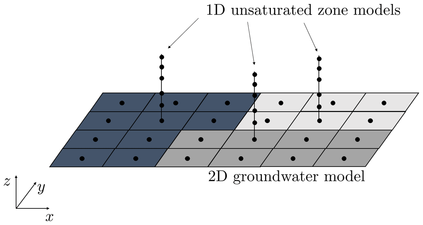
Figure 1 Example of the coupled model grid with three recharge zones (white, gray and black).

Both components are discretized using finite volumes and an implicit Euler time integration. The nonlinear systems of equations are solved using the Newton–Raphson scheme and line search. For the groundwater model, a rectangular grid with uniform grid spacing is used. The 1D grid for the unsaturated zone can be non-uniform.

The boundary conditions on the lateral sides of the groundwater model can be either Neumann or Dirichlet boundary conditions. The upper boundary condition of the unsaturated zone models is a Neumann boundary representing the flux across the land surface. In this work, the flux will be either precipitation or the net flux from precipitation and evapotranspiration depending on the test case. The feedback from the groundwater model to the unsaturated zone models as well as the lower boundary condition of the unsaturated zone models depends on the coupling method described in the following sections.

The time step size of the unsaturated zone model is smaller than that of the groundwater model to guarantee convergence in the former but also numerical efficiency for the full model. The coupling time step, which defines the interval when the two model components exchange their information, is equal to the time step size of the groundwater model. All exchanged information such as groundwater recharge is assumed to be constant during one coupling time step.

Both components as well as the coupling routine are implemented in MATLAB.

2.2.2 Non-iterative method

The first coupling method aims at providing a fast and iterative-free (but also rather approximate) solution to the numerical problem. A previous version of the model is published in Erdal et al. (2019). In this method, specific yield is a parameter of the groundwater model that the user needs to specify during model setup. Each unsaturated zone column is set up to range from the groundwater table to the land surface, with a Dirichlet boundary h=0 m at the bottom. A coupling time step is then performed as follows:

1. Run all unsaturated 1D column models for the coupling time step, collect the computed recharge (i.e., fluxes leaving over the bottom boundary for all 1D time steps during the coupling time step) and interpolate the 2D map of groundwater recharge.

2. Run the 2D groundwater model for the coupling time step with the computed recharge.

3. For each 1D column, resize all cells by a uniformed ratio computed such that the resized grid fits the new groundwater table to land surface distance at the column location. Thus, the cell sizes Δz are changed while all other properties of the model are kept as they are, including saturation and hydraulic head which means a gain or loss of water in the 1D models.

4. Compute the amount of water lost (or gained) in each unsaturated model by resizing the grid.

5. Add (or subtract) a ratio r of this water to the recharge computed in the next coupling time step.

6. Move to the next coupling time step and repeat from point 1.

The ratio r can in principle range from 0 to 1. At 1 the coupled model is locally mass conservative, as no water is lost or gained during the grid resizing. However, a local mass-conservation in a non-iterative coupling method may not be wanted. Reasons for this are, for example, (1) the water content in the unsaturated zone is also effected by lateral flows in the groundwater, (2) the added or subtracted water is only added in the next time step, (3) the dynamics around the rising or falling groundwater table is only captured in rough terms, and (4) the column resizing is distributed across the full column. This can cause numerical problems like oscillating groundwater tables. In this work we compute r as the ratio between the incoming water volume from the 1D column (RΔt_c [m]) and the volume of water added to (or subtracted from) the groundwater (ϕ⋅ΔH_GW [m]):

$$\begin{array}{}\text{(6)}& r_i=min\left\{\left|{\displaystyle \frac{R_i\mathrm{\Delta }{t}_{\mathrm{c}}}{{\mathit{\varphi }}_i\mathrm{\Delta }{H}_{\mathrm{GW},i}}}\right|,\mathrm{1}\right\},\end{array}$$

where i is the index of the column, Δt_c [s] is the coupling time step and r is limited to a maximum value of 1. The current formulation gives an indication to what extent the change of groundwater elevation can be attributed to the incoming groundwater recharge. If recharge is the main contribution, the water lost or gained in the resizing could be assumed to have entered or left the groundwater, while if the recharge is small but the change in groundwater table large, we find it more likely that the water may still be in the unsaturated zone. We note that this is an ad hoc solution and that it differs to the one presented in Erdal et al. (2019), where r was simply set to 0. However, numerical tests show good stability and the best overall performance for the applied test cases when r is computed as in this work even though a value of r=1 would be needed to keep strict mass conservation.

2.2.3 Iterative method

The second method couples the groundwater and the unsaturated model parts iteratively. Here, the 1D soil columns span the entire soil thickness from the impervious bottom of the aquifer up to the land surface. Thus, the 1D and the 2D model overlap in the saturated part. The bottom boundary condition of the 1D columns is then a no-flow boundary.

The groundwater recharge R [ms⁻¹], that is passed from the unsaturated zone models to the groundwater model, is defined – similar as in Crosbie et al. (2005) – as the amount of water being added to or subtracted from the groundwater over time and calculated from each unsaturated flow model as

$$\begin{array}{}\text{(7)}& R^{\mathit{\nu }}={\displaystyle \frac{\mathrm{\Delta }{H}_{\mathrm{UZ}}^{\mathrm{1}}\cdot S_{\mathrm{y}}^{\mathit{\nu }}}{\mathrm{\Delta }{t}_{\mathrm{c}}}},\end{array}$$

where H_UZ [m] is the position of the groundwater table in the unsaturated zone model, S_y [–] is the specific yield, Δt_c [s] is the coupling time step and the superscript (ν) is the iteration counter for the coupling time step loop.

The information passed from the groundwater model to the unsaturated zone models is the lateral fluxes Q_lat [ms⁻¹] into or out of the columns cells. These data are calculated at the locations where the unsaturated and groundwater models overlap as the amount of water being added to or subtracted from the groundwater over time minus recharge:

$$\begin{array}{}\text{(8)}& Q_{\mathrm{lat}}^{\mathit{\nu }}={\displaystyle \frac{\mathrm{\Delta }{H}_{\mathrm{GW}}^{\mathit{\nu }-\mathrm{1}}\cdot S_{\mathrm{y}}^{\mathit{\nu }-\mathrm{1}}}{\mathrm{\Delta }{t}_{\mathrm{c}}}}-R^{\mathit{\nu }-\mathrm{1}},\end{array}$$

with H_GW [m] being the position of the groundwater table in the groundwater model. This cumulative flux is spread over the saturated part of the corresponding 1D model by taking into account the variable cell sizes of the 1D grid:

$$\begin{array}{}\text{(9)}& q_{\mathrm{lat},i}^{\mathit{\nu }}=Q_{\mathrm{lat}}^{\mathit{\nu }}\cdot {\displaystyle \frac{\mathrm{\Delta }{z}_i}{{\sum }_j\mathrm{\Delta }{z}_j}}\text{with}{z}_i,z_j\le H_{\mathrm{UZ}}.\end{array}$$

The local flux q_lat,i [ms⁻¹] is given as a source or sink term to the ith cell of the 1D model. This procedure is shown exemplarily for one 1D model in Fig. 2.

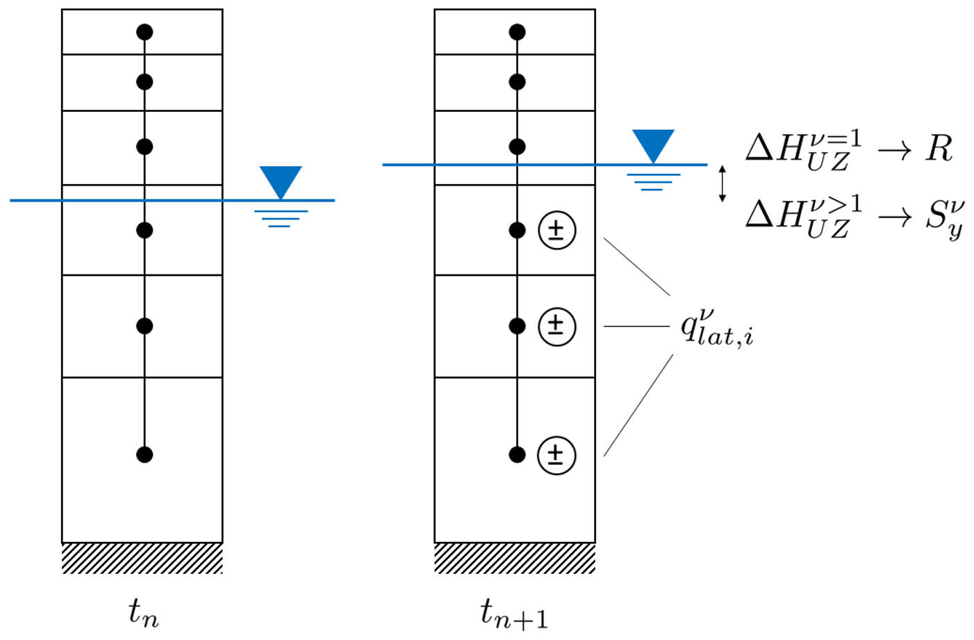
Figure 2 Illustrative example of the time step integration for one 1D model in the iteratively coupled model.

In this approach, the position of the groundwater table in both models is not used as exchange information but as closure criterion for the iteration. With the lateral fluxes from groundwater flow being accounted for in the unsaturated zone models, the calculated groundwater table position at the next time step should be equal in both models. However, this is only the case if the specific yield is chosen to correctly represent the behavior of the unsaturated zone in the groundwater model. As was already discussed in the introduction, the specific yield is dynamic. Therefore, it needs to be determined at every time step. In the literature, different approaches of how to define and calculate the specific yield can be found. Most of them lack the dependency on the fluctuations of the groundwater table ΔH. The method proposed by Zeng et al. (2019) takes this into account but requires the definition of a threshold elevation above the groundwater table. Here, we propose a method that calculates the specific yield depending on ΔH without the need for further user-defined parameters:

$$\begin{array}{}\text{(10)}& S_{\mathrm{y}}^{\mathit{\nu }}={\displaystyle \frac{Q_{\mathrm{lat}}^{\mathit{\nu }}\cdot \mathrm{\Delta }{t}_{\mathrm{c}}}{\mathrm{\Delta }{H}_{\mathrm{UZ}}^{\mathit{\nu }}-\mathrm{\Delta }{H}_{\mathrm{UZ}}^{\mathrm{1}}}}.\end{array}$$

It represents the ratio of the lateral fluxes and the corresponding change of the groundwater table position in the unsaturated zone model. In our case this is equivalent to relating all incoming fluxes ($Q_{\mathrm{lat}}^{\mathit{\nu }}+R^{\mathit{\nu }}$) to the total change of the groundwater table position ($\mathrm{\Delta }{H}_{\mathrm{UZ}}^{\mathit{\nu }}$). So the specific yield is no longer a fixed model parameter but the ratio of the calculated water gain or loss per calculated groundwater level change where the water level change is calculated using the 1D Richards equation, which does not have the specific yield as a parameter. We thereby to a certain extent impose the unsaturated zone model upon the groundwater model. As the altered specific yield may lead to different lateral fluxes and consequently to a different specific yield, several iteration steps are needed to achieve a consistent solution in both model compartments. The convergence of the specific yield is – as in any numerical scheme – bound to an adequate choice of the numerical grid and in this case additionally to a sufficient number of unsaturated zone models which can both be found by a convergence study. Note that if $\mathrm{\Delta }{H}_{\mathrm{UZ}}^{\mathit{\nu }}-\mathrm{\Delta }{H}_{\mathrm{UZ}}^{\mathrm{1}}=\mathrm{0}$m, then there are no lateral fluxes, which means that there is no iteration required and that the specific yield stays at its current value.

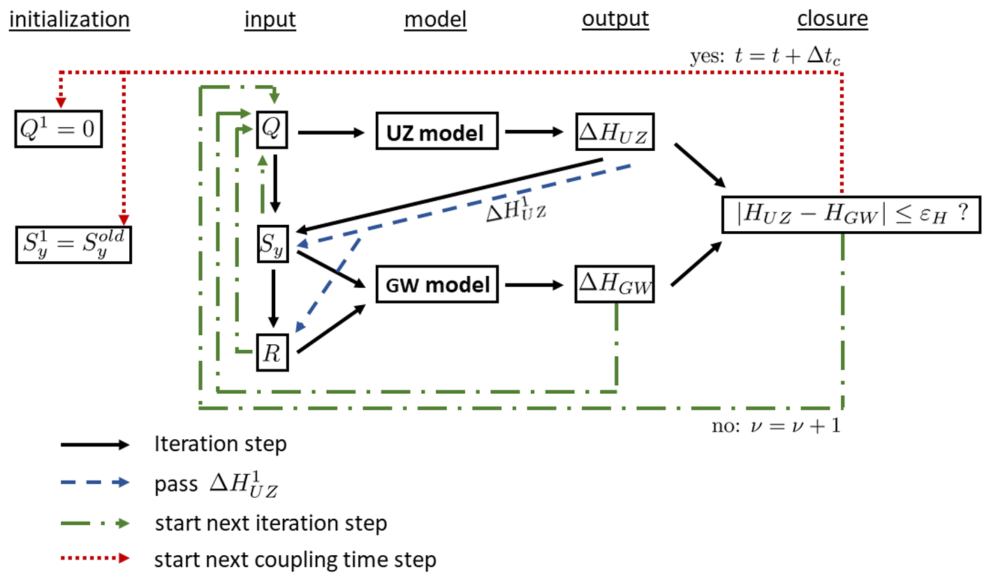
The integration of the coupled model to the next time step, which is illustrated in Fig. 3, can be thus summarized as follows:

1. Run all unsaturated 1D column models for the coupling time step with $q_{\mathrm{lat},i}=\mathrm{0}$ms⁻¹ ∀i, calculate the computed recharge according to Eq. (7) and interpolate the 2D map of groundwater recharge R¹.

2. Run the 2D groundwater model for the coupling time step with the computed recharge R¹.

3. Calculate the lateral flux source or sink terms $q_{\mathrm{lat},i}^{\mathit{\nu }}$ for the 1D models (Eq. 9).

4. Run all unsaturated 1D column models for the coupling time step with $q_{\mathrm{lat},i}^{\mathit{\nu }}$, calculate the computed recharge according to Eq. (7) and interpolate the 2D map of groundwater recharge R^ν.

5. Calculate and interpolate the 2D map of specific yield $S_{\mathrm{y}}^{\mathit{\nu }}$ using Eq. (10).

6. Run the 2D groundwater model for the coupling time step with the updated recharge R^ν and specific yield $S_{\mathrm{y}}^{\mathit{\nu }}$.

7. Repeat steps 3 to 6 until $|H_{\mathrm{UZ}}^{\mathit{\nu }}-H_{\mathrm{GW}}^{\mathit{\nu }}|\le {\mathit{\epsilon }}_H$.

8. Move to the next coupling time step and repeat from point 1.

Note that an assumption is made in this approach. The source or sink terms q_lat,i have an effect on the recharge ($R(Q_{\mathrm{lat}}=\mathrm{0})\ne R(Q_{\mathrm{lat}}\ne \mathrm{0})$), which due to the nonlinearity of the Richards equation cannot be quantified. This effect is assumed to be negligible, and the fluctuations due to recharge ($\mathrm{\Delta }{H}_{\mathrm{UZ}}^{\mathrm{1}}$) are kept constant during the iterations, whereas the remainder of the total fluctuations ($\mathrm{\Delta }{H}_{\mathrm{UZ}}^{\mathit{\nu }}-\mathrm{\Delta }{H}_{\mathrm{UZ}}^{\mathrm{1}}$) are assigned entirely to the lateral fluxes. Changes of the recharge R^ν during the iteration are then only caused by changes in the specific yield (see Eq. 7).

Besides, as groundwater recharge and specific yield are calculated from the unsaturated zone models, they are spatially uniform for all cells of the groundwater model that belong to the zone assigned to that unsaturated zone model. This leads to a simplified recharge and specific yield pattern but is necessary to keep the model computationally efficient.

Figure 3 Flow diagram for the iterative coupling.

2.3 Activity scores

We perform a global sensitivity analysis to identify the most influential parameters for the groundwater dynamics in the coupled model. As metric, we use activity scores (Constantine and Diaz, 2017). For this, we define the vector of m model parameters x normalized to a range of [0,1] with the probability density function ρ(x) of the parameters and the scalar model output f(x). In our case, the parameters are the soil hydraulic parameters and the upper boundary condition, defined in more detail in Sect. 3.4. The model output f is either the groundwater table position, its daily fluctuation or the calculated specific yield in the iterative model (see Sect. 4.4).

The active subspace of f is defined by the eigenvectors of the matrix

$$\begin{array}{}\text{(11)}& \mathbf{C}=\int \mathrm{\nabla }f\left(\mathit{x}\right)\mathrm{\nabla }f\left(\mathit{x}{)}^T\mathit{\rho }\right(\mathit{x})\mathrm{d}\mathit{x}=\mathbf{W}\mathrm{\Lambda }{\mathbf{W}}^T,\end{array}$$

where W is the matrix of eigenvectors, and Λ is the diagonal matrix of the corresponding eigenvalues λ_i in decreasing order. If there exists a λ_n that fulfills ${\mathit{\lambda }}_n\gg {\mathit{\lambda }}_{n+\mathrm{1}}$, Λ and W can be partitioned into

$$\begin{array}{}\text{(12)}& \mathrm{\Lambda }=\left[\begin{array}{cc}{\mathrm{\Lambda }}_{\mathrm{1}}& \\ & {\mathrm{\Lambda }}_{\mathrm{2}}\end{array}\right]\text{and}\mathbf{W}=\left[\begin{array}{cc}{\mathbf{W}}_{\mathrm{1}}& {\mathbf{W}}_{\mathrm{2}}\end{array}\right],\end{array}$$

with Λ₁ containing the first n eigenvalues on its diagonal and W₁ consisting of the first n columns of W. The column span of W₁ is the active subspace of dimension n of the function f. The product ${\mathbf{W}}_{\mathrm{1}}^T\mathit{x}$ gives the n first active variables which are linear combinations of the normalized input parameters. A variation of an active variable causes a stronger variation in f(x) than a variation of the inactive variables given by ${\mathbf{W}}_{\mathrm{2}}^T\mathit{x}$. Then, the individual sensitivity for the ith parameter can be calculated as

$$\begin{array}{}\text{(13)}& a_i=a_i\left(n\right)=\sum _{j=\mathrm{1}}^n{\mathit{\lambda }}_j{w}_{ij}^{\mathrm{2}},\end{array}$$

where λ_j is the jth eigenvalue, and w_ij is the value corresponding to the ith parameter in the jth eigenvector. This metric is called the activity score. For a transient problem, the activity score of a parameter can change with time, leading to a transient activity score a_i(t).

In this work, the activity score is computed independently for each time step to create a transient score and normalized such that the sum of all scores at one time step is equal to one:

$$\begin{array}{}\text{(14)}& {\mathrm{NAS}}_i\left(t\right)={\displaystyle \frac{a_i\left(t\right)}{{\sum }_{i=\mathrm{1}}^m{a}_i\left(t\right)}}.\end{array}$$

Often, the integration over the parameter space required in Eq. (11) is not feasible or not possible. Therefore, a Monte Carlo method, where M samples are drawn independently from ρ(x), is used to compute the matrix C as proposed in Constantine et al. (2015):

$$\begin{array}{}\text{(15)}& \mathbf{C}\approx {\displaystyle \frac{\mathrm{1}}{M}}\sum _{i=\mathrm{1}}^M\mathrm{\nabla }f\left({\mathit{x}}_i\right)\mathrm{\nabla }f({\mathit{x}}_i{)}^T.\end{array}$$

Another issue is related to the determination of ∇f. As this gradient is often unavailable, a common approach is to fit a polynomial model to relate the model output to the input parameters (Jefferson et al., 2015; Erdal and Cirpka, 2019). Following the suggestion by Erdal and Cirpka (2019), a second-order polynomial depending on the input parameters is fitted to the data f(x) using standard multiple regression, from which the gradient ∇f can be computed easily:

$$\begin{array}{}\text{(16)}& f\left(\mathit{x}\right)\approx b_{\mathrm{0}}+\sum _{i=\mathrm{1}}^m{b}_i{x}_i+\sum _{i=\mathrm{1}}^m\sum _{j=\mathrm{1}}^m{b}_{ij}{x}_i{x}_j.\end{array}$$

3 Test cases

We test and compare the above described coupling methods using three different test cases. The first two test cases are taken from Beegum et al. (2018) where the second one was originally set up by Morway et al. (2013). As these are rather artificial, we added a third test case which is more complex and more realistic. The first test case is a flow model in a bucket setup where all boundary sides are closed. It represents a 1D flow problem consisting of two homogeneous soil layers with dynamic precipitation evapotranspiration (P-ET) data. It is used to investigate the coupling in the absence of any lateral fluxes where fluctuations of the groundwater table are only due to groundwater recharge. The second test case is conceptualized with a 3D model domain. However, as all parameters are constant over the length of the domain, it is effectively a 2D flow problem. Here again the soil is homogeneous, but it contains lateral fluxes. The third test case is similar to the second but the dimensions and the precipitation are modified such that the groundwater table falls during a certain period and the soil is made heterogeneous. This test case is a true 3D flow problem. The main features of the test cases are summarized in Table 1. For the 1D bucket model, one 1D soil column that is not coupled to groundwater is solved for comparison. The results of the other two test cases are compared to those obtained from a fully integrated 3D model set up with Parflow (Kollet and Maxwell, 2006).

Table 1 Main features of the three test cases.

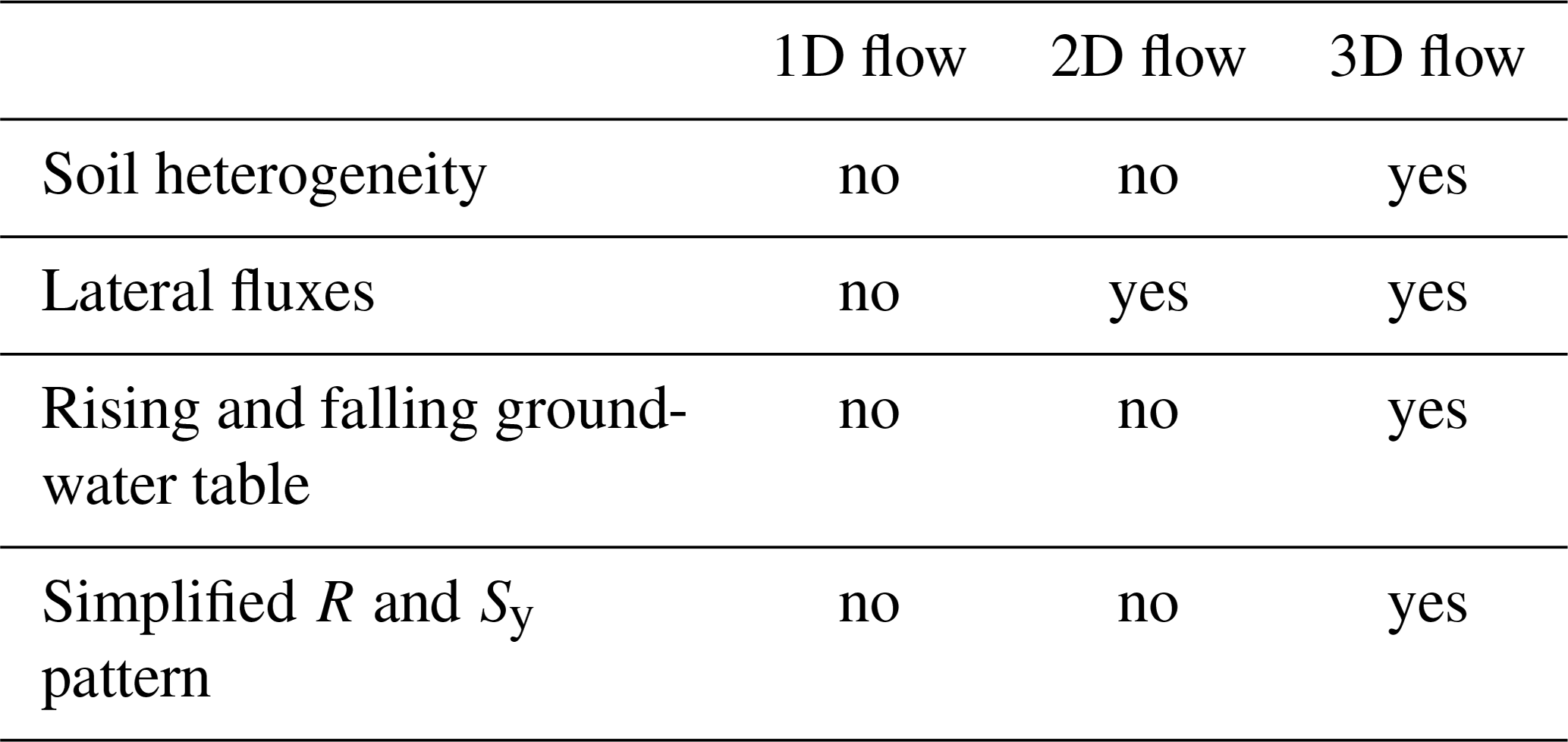
Table 2 Soil hydraulic parameters for the three test cases for Parflow and the coupled model.

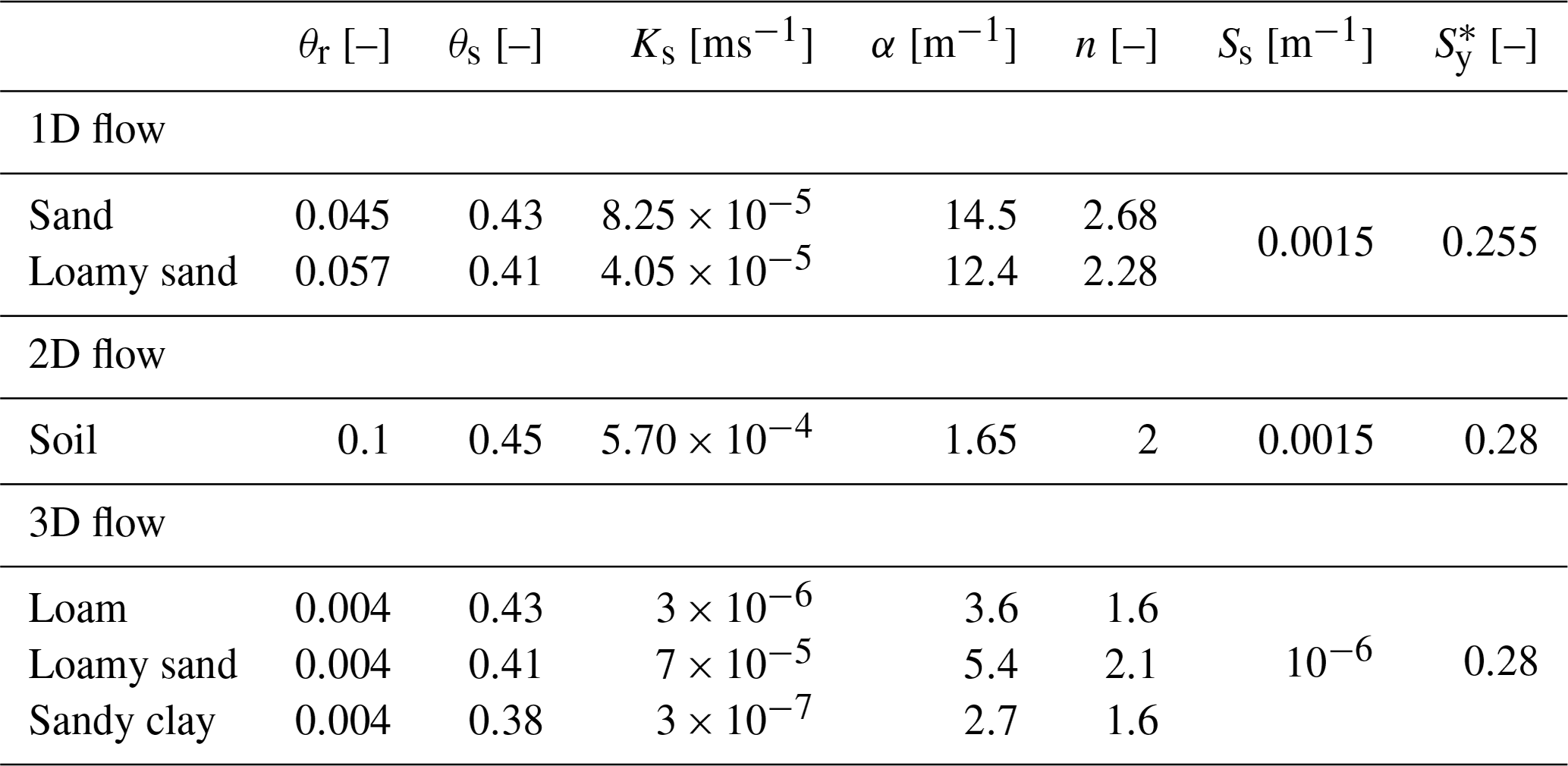
^* Only needed in the coupled model. Using the iterative coupling, this value is the initial value $S_{\mathrm{y}}^{\mathrm{0}}.$

For the global sensitivity analysis, a fourth test case is created which is mainly a combination of the second and the third test case. They are combined and modified in such a way that the groundwater table rises and falls, the simulation is long enough to finish the model spin-up and parameters are homogeneous within each model compartment.

We performed a convergence study on the spatial grid resolution (Δx=Δy and Δz) and coupling time step size (Δt_c) for the three applied test cases using the iteratively coupled model. As we want to compare our results to those of Beegum et al. (2018), we chose the grid sizes corresponding to the accuracy we obtained for the grid resolution used in their work (mean absolute error of the groundwater table over time of $\mathrm{MAE}\le \mathrm{5}\times {\mathrm{10}}^{-\mathrm{3}}$m) for our final calculations. To guarantee the comparability among the fully integrated and the coupled model, we always use the same grid for the reference and for the coupled model using the two coupling schemes although one has to keep in mind that the vertical grid resolution in the non-iteratively coupled model will change during the remeshing. The convergence study showed that in the vertical direction a much finer grid is needed with form factors up to 500. Besides, the third (heterogeneous) test case requires a finer horizontal grid to achieve the same accuracy as in the other two test cases. For all three test cases, the influence of the coupling time step Δt_c was negligible. Therefore, we decided to use the maximal possible value Δt_c=1 d (as we have daily changing forcing data in test case 1) for all test cases. The grid for the fourth test case used for the sensitivity analysis was not determined from a convergence study since its accuracy does not need to be comparable to the other test cases and since the convergence study might show different results for different parameter combinations. Instead, we chose a grid resolution between the second and the third test case, of which this test case is a mixture.

3.1 Test case 1: 1D flow

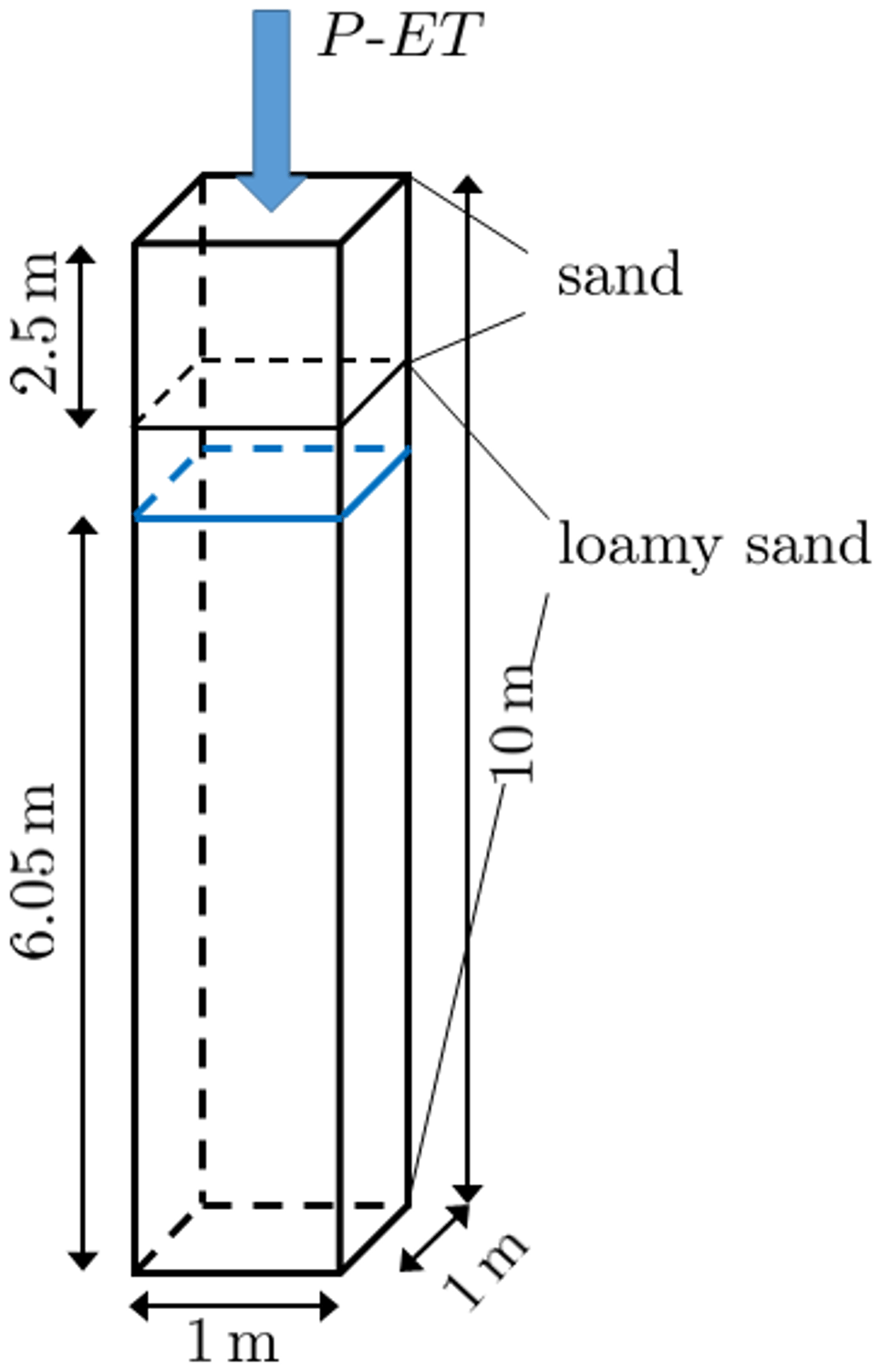
This model is taken from Beegum et al. (2018) and covers a domain of 1 m × 1 m  × 10 m. All lateral boundaries are no-flow boundaries. The net flux of daily varying precipitation and evapotranspiration (P-ET) shown in Fig. 4 is applied as a Neumann boundary at the soil surface. These data were collected at a weather station in Gdańsk, Poland, in 2011. The initial condition assumes a hydrostatic pressure profile in the lower 6.5 m of the soil corresponding to an initial position of the groundwater table at 3.95 m below the surface. In the upper 3.5 m of the soil, unit gradient flow is imposed by setting the pressure head to −0.283 m. The soil consists of two layers: a sandy soil in the top 2.5 m and a loamy sand soil underneath (see Fig. 5). The soil hydraulic parameters for the two layers are given in Table 2. Since the groundwater table stays below the interface to the sandy soil layer during the entire simulation, the groundwater model is assigned the loamy sand parameters.

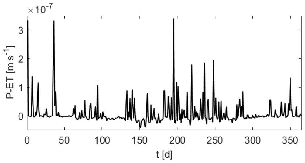
Figure 4 Net precipitation and evapotranspiration used for the 1D flow model. Positive values indicate inflow and negative values outflow.

Figure 5 Model domain and initial water table position for the 1D flow model.

The total simulation time is 1 year. The 1D model used for comparison (pure Richards model, not coupled to groundwater) uses an adaptive time stepping scheme with a minimum value of 1 s and a maximum value of 1 h. The grid is uniform with 1000 cells of 0.01 m height. The same spatial resolution is used for the 1D models in the coupled model. The groundwater domain is divided into a 2×2 grid. Each groundwater cell is assigned a 1D model. The coupling time step as well as the time step of the groundwater model is set to 1 d for both coupling methods. The time step for the 1D models is adaptive with a minimum value of 1 s and a maximum value of 1 d.

3.2 Test case 2: 2D flow

The dimensions of this model (Morway et al., 2013; Beegum et al., 2018) are 8000 m × 4000 m × 15 m. Since there is no variability along the 8000 m side, flow is effectively 2D in this test case. There is a constant slope of 0.1 % at the 4000 m side. Two no-flow boundaries are assigned along the shorter side walls. On the other two sides there are Dirichlet boundaries corresponding to a groundwater table elevation of H=7 m and H=0.9 m at the top and the bottom of the slope, respectively (Fig. 6). The initial groundwater table elevation is interpolated linearly between the two Dirichlet boundaries. The initial condition for the 1D models is generated by applying hydrostatic equilibrium and assigning a minimal initial pressure head of −1.25 m at locations where the pressure head is below this value. Monthly varying rainfall (Fig. 7) is used as Neumann boundary condition for the land surface. The forcing is repeated for five cycles summing up to a total simulation time of 5 years. The soil parameters are listed in Table 2.

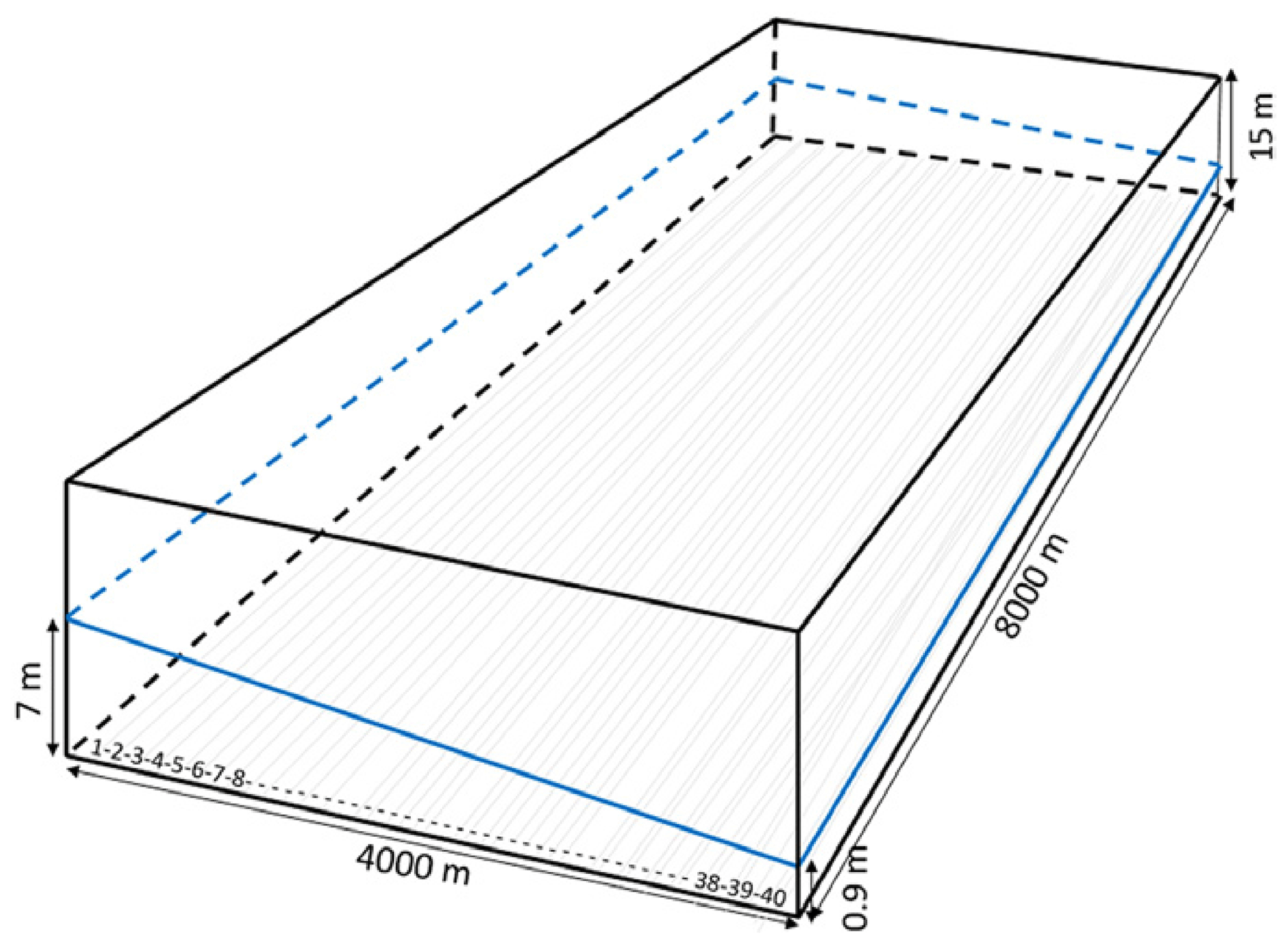
Figure 6 Model domain and initial water table position for the 2D flow model (Beegum et al., 2018).

Figure 7 Net inflow used for the 2D flow model.

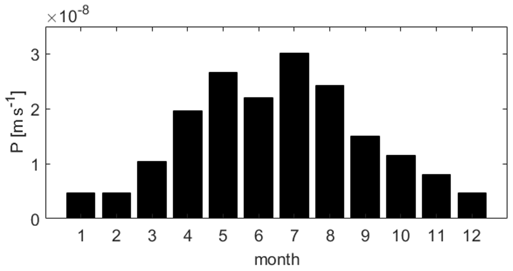
The 3D Parflow reference model uses a uniform grid with $\mathrm{80}\times \mathrm{40}\times \mathrm{75}$ cells with grid size $\mathrm{\Delta }x=\mathrm{\Delta }y=\mathrm{100}$m and Δz=0.2 m. The spatial resolution in the coupled model is the same with a 80×40 grid for the groundwater model and 75 cells for the unsaturated zone models. The groundwater domain is divided into 40 zones all consisting of slices along the 8000 m side as shown in Fig. 6. With the flow problem being 2D, this means that the entire domain is actually covered by 1D models. The coupling and groundwater time step is Δt_c=1 d, and the time step for the 1D models is again adaptive with a minimum value of 1 s and a maximum value of 1 d. Parflow uses an adaptive time scheme as well, with a maximum value of 1 h.

3.3 Test case 3: 3D flow

The first two test cases are rather simple. Therefore, a third test case is designed where the properties that are relevant for the coupling are closer to those of a model for a real hydrological system. The setup is similar to that of the second test case but with some modifications. The domain size is reduced to 800 m × 400 m × 15 m, and the slope is maintained. The lateral boundaries are the same: the flux boundary at the land surface now consists of three cycles of the precipitation shown in Fig. 7, followed by 2 no-flux years and then again 2 years using the original precipitation data. Thus, the total simulation time is 7 years. With these changes, the groundwater table is forced to eventually fall and then rise again. Apart from the more dynamic groundwater table, the influence of heterogeneities should be investigated with this test case. Therefore, instead of the homogeneous soil, three different soil types, representing loam, loamy sand and sandy clay, are distributed throughout the domain as depicted in Fig. 8. The distribution is synthetic and the corresponding parameter values are given in Table 2. In the coupled model, the parameters for the groundwater model are averaged arithmetically over the depth of the saturated zone in that grid cell. This averaging takes place at every time step adapting to the new position of the groundwater table. The initial condition is the same as in the 2D flow case.

Figure 8 Distribution of soil types along the 800 m side at x=195 m in the 3D flow model. gray: loam, white: loamy sand, black: sandy clay.

The horizontal spatial resolution is increased to $\mathrm{\Delta }x=\mathrm{\Delta }y=\mathrm{5}$m. The vertical grid consists of 200 cells and is non-uniform with grid sizes ranging between Δz_min=0.75 mm at the surface and Δz_max=0.3 m at the bottom. The same resolution is used for Parflow and for the coupled model. With the heterogeneous soil, each grid cell of the groundwater model would need a 1D model to cover the entire domain. As this is computationally not feasible, the groundwater domain is again divided into 40 zones but now spread evenly across the domain each covering an area of 20×16 grid cells. The 1D models are placed at the center of each zone and assigned the soil hydraulic parameters at this location. Thus, also the influence of a simplified recharge (and specific yield) pattern, which is constant within each zone and calculated from the corresponding 1D model, can be investigated. The time step sizes are the same as in the 2D flow model.

3.4 Test case 4: sensitivity analysis

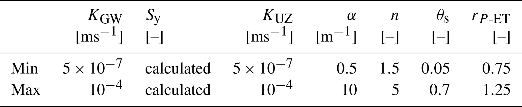
As already pointed out, for this test case the 2D and 3D flow test cases were combined. The domain size and the boundary conditions as well as the initial condition are the same as in the 3rd test case. This was done to maintain the rising and falling groundwater table. To get rid of spin-up effects, the simulation time was increased, running four times the precipitation data used for the 3D flow case, adding up to a total simulation time of 28 years. The soil structure was simplified to be homogeneous within each model compartment, i.e., the groundwater model and the unsaturated zone models. For a heterogeneous soil structure, a global sensitivity analysis would not be feasible nor very meaningful. The parameters included in the sensitivity analysis are listed in Table 3. Here, K_GW and K_UZ are the saturated hydraulic conductivity of the groundwater model and the unsaturated zone models, respectively, whereas the saturated part of the 1D models, that overlaps with the groundwater model, is also assigned the K_GW value. This means that the hydraulic conductivity of an unsaturated model cell is changed when the cell becomes saturated or unsaturated. Thus, inconsistencies between the two model compartments that may lead to numerical problems are avoided. The parameters are sampled from uniform distribution functions ρ to cover their entire physically plausible range. Table 3 shows the limits of these ranges. Additionally, the influence of the upper boundary condition is investigated by multiplying the precipitation data with a constant factor r_P-ET. The residual saturation $S_{\mathrm{r}}={\mathit{\theta }}_{\mathrm{r}}/{\mathit{\theta }}_{\mathrm{s}}$ and the specific storage S_s are excluded from the analysis and set to 0.01 and 0.0015, respectively, as a previous smaller sensitivity analysis had shown no impact of these parameters (not shown). The specific yield values are calculated by the model, so the range is defined by these calculated values. Even though this is not a predefined parameter, its influence on the model output, i.e., the groundwater table dynamics, is of great interest and should be comprehensible and consistent over the entire simulation time.

Table 3 Parameter ranges for the parameters included in the sensitivity analysis. For the saturated hydraulic conductivity, values for the groundwater (GW) and the unsaturated zone (UZ) model as well as the van Genuchten α the normal logarithm are sampled.

The horizontal spatial resolution is $\mathrm{\Delta }x=\mathrm{\Delta }y=\mathrm{10}$m, and the vertical resolution is Δz=0.1 m. As the sensitivity analysis requires a lot of model realizations, the number of unsaturated zone models and corresponding zones is decreased to eight to save computation time. Similar to the second test case, they are placed evenly along the 800 m side of the domain since the soil is homogeneous and flow thus 2D again. The time step sizes are the same as in the previously described test cases.

4 Results and discussion

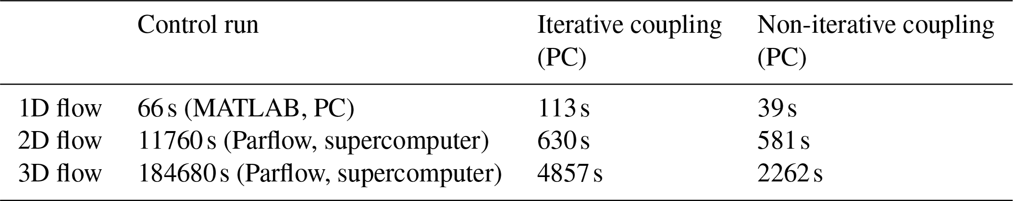
The coupling methods are compared in terms of accuracy and efficiency. The spatial and temporal distribution of the groundwater table is used for the evaluation of the accuracy. The wall clock time serves as indicator for speed and is given in Table 4. No information about run times are given in Beegum et al. (2018). Therefore, their results are not included in the speed comparison. All MATLAB calculations are done on a local desktop PC with an Intel Core i5 using two cores for the coupled model runs. The Parflow runs used for the other test cases are performed on the JUWELS supercomputer at the Research Centre Jülich which provides 2567 compute nodes with Dual Intel Xeon CPUs. Twelve cores were used for the simulations.

Table 4 Wall clock times for the different test cases and coupling schemes.

The iterative coupling uses a dynamic formulation of the specific yield. The resulting values are investigated in terms of plausibility. The groundwater table position, the groundwater table fluctuations and the specific yield calculated from the iterative coupling (all taken at the center of the domain) are used as observations f(x) for the global sensitivity analysis. The resulting transient activity scores (Eq. 14) of the parameters listed in Table 3 are analyzed to identify the most influential parameters and to see whether the calculated specific yield behaves reasonably.

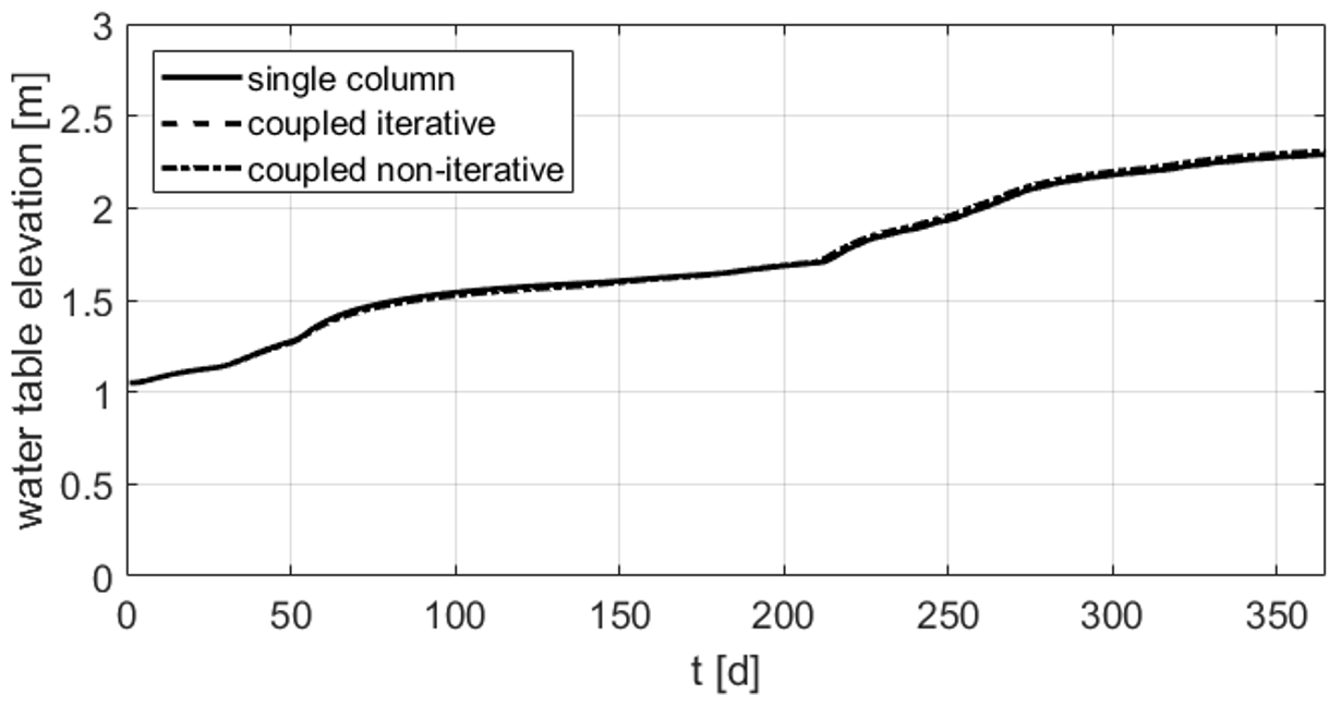
4.1 Results 1D flow

Figure 9 shows the water table elevation over time for the single column reference run and the two coupling schemes. The reference elevation z=0 m is located at 5 m below the surface. This is done to facilitate the comparison to the work by Beegum et al. (2018). Both the iterative and the non-iterative coupling scheme show a good match with the single column run. The accuracy of the iterative approach is slightly higher; no difference to the single column run can be seen in Fig. 9. A visual comparison indicates that the coupling applied by Beegum et al. (2018) yields a comparable accuracy.

The dynamic adaptation of the specific yield in the iterative coupling scheme is active only in the presence of lateral fluxes, because otherwise due to the formulation of the recharge in Eq. (7) the groundwater table fluctuations in the two model compartments are already forced to be the same in the first iteration step. Therefore, in this test case the value stays constant at its initial value, and further investigation is not possible.

Figure 9 Groundwater table elevation over time for the 1D flow problem.

For the 1D flow problem, the iterative coupling takes roughly three times as much wall clock time as the non-iterative coupling (see Table 4). This is due to the larger grid of the iterative model which also includes the saturated part.

4.2 Results 2D flow

The temporal evolution of the groundwater table position at the center of the domain is shown in the upper plot of Fig. 10. While both coupling approaches tend to overestimate the elevation of the groundwater table, increasing with time, the non-iterative coupling shows a rather large offset compared to the Parflow run. This difference is also evident in the spatial plot of the groundwater table in the lower part of Fig. 10. The overestimation of the iterative coupling scheme is also visible there but is clearly smaller. Besides, there is a shift in the shape of the groundwater table. The iterative coupling scheme shows the largest difference to the Parflow model close to the boundary at x=4000 m which will be discussed further in Sect. 4.5. The largest difference between the non-iterative coupling and the Parflow run occurs at around x=1000 m. The results by Beegum et al. (2018) have a similar accuracy and shape as the results of the iterative coupling approach.

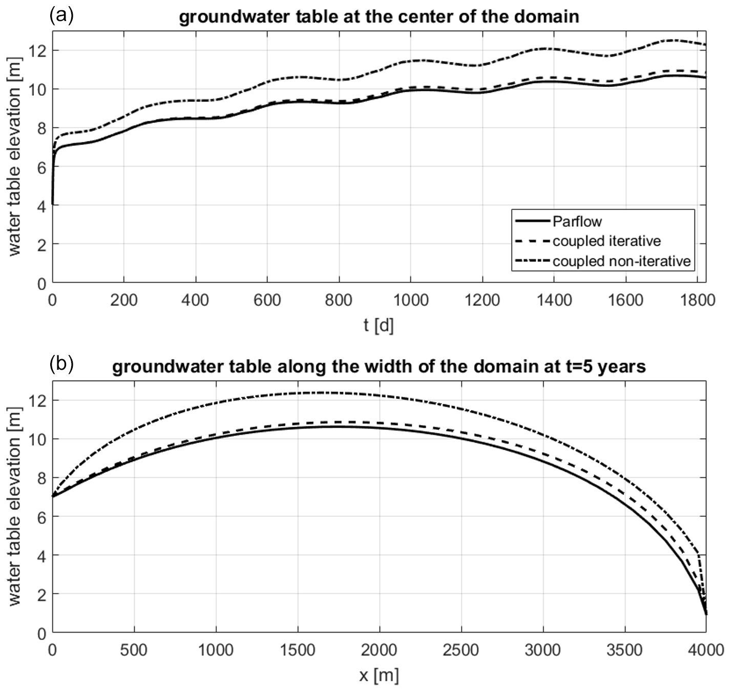
Figure 10 Results of the 2D flow problem. (a) Groundwater table elevation over time in the center of the domain. (b) Groundwater table along the width of the domain at the final time step.

When considering the non-iterative model, it is notable that initial time steps are an issue, as the model starts almost immediately with a too high groundwater table. However, the difference also grows slowly over time. Both of these issues occur as well when using smaller time step sizes and may be related to the reference model essentially acting as a bucket without any plausible steady-state solution (i.e., steady state for the groundwater model would have groundwater tables far above the top of the domain). As such, an initial error in the model can never be compensated and will also lead to feedback effects, such as an overestimation of the groundwater recharge due to too short unsaturated zone model columns. In this respect, the 2D flow test case is of limited use when evaluating simplified models for realistic setups.

The lateral fluxes in this setup cause a temporally and spatially changing value of the specific yield in the iterative model, which can be seen in the left plot of Fig. 11. However, the differences among the predefined zones (different lines) and also the temporal fluctuations are rather small. All values are smaller than the proposed value of 0.28, although the difference is less than 0.03. The temporal fluctuations of S_y suggest a dependence on the fluctuations of the groundwater table which also show a repeating pattern due to the cyclic forcing, whereas its spatial differences indicate the dependence on the water table position. The right plot of Fig. 11 shows the specific yield over the groundwater table position. The least squares regression line reveals a linear relationship between these two variables, where S_y is increasing with increasing H_GW. Nevertheless, the temporal and the spatial differences of S_y are small here, which might be due to the homogeneity of the soil.

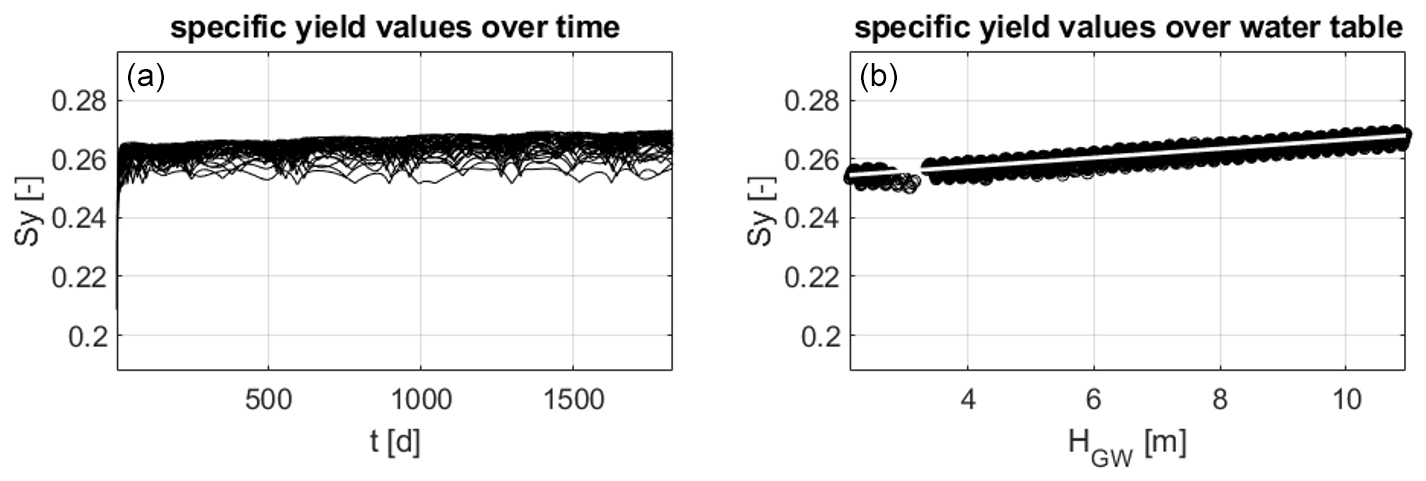
Figure 11 Specific yield values resulting from the iterative coupling for the 2D flow problem. (a) Specific yield over time. Each line corresponds to a 1D model and zone of equal recharge and specific yield in the groundwater model. (b) Specific yield over groundwater table position. The white line is the least squares regression line.

For this setup, again the non-iterative coupling is faster than the iterative coupling (see Table 4), but the difference is very small, especially compared to the high run time used for the full 3D Parflow model.

4.3 Results 3D flow

In Fig. 12 the position of the groundwater table at the center of the domain is plotted over time (upper part). Both coupling schemes show a good agreement with the fully integrated 3D model. Similar behavior is found at other positions in the domain. The non-iterative scheme has a slight delay when the groundwater table is rising more rapidly, e.g., around t=1000 d and t=2250 d. The groundwater table along the width of the domain (y=400 m) at the end of the simulation is plotted in the lower part of Fig. 12. Again, both coupling approaches match the Parflow result very well with small differences between x=300 m and x=370 m. The mismatch between the fully integrated and the coupled model is even smaller than in the less complex 2D flow case, which will be explained in the discussion part (Sect. 4.5).

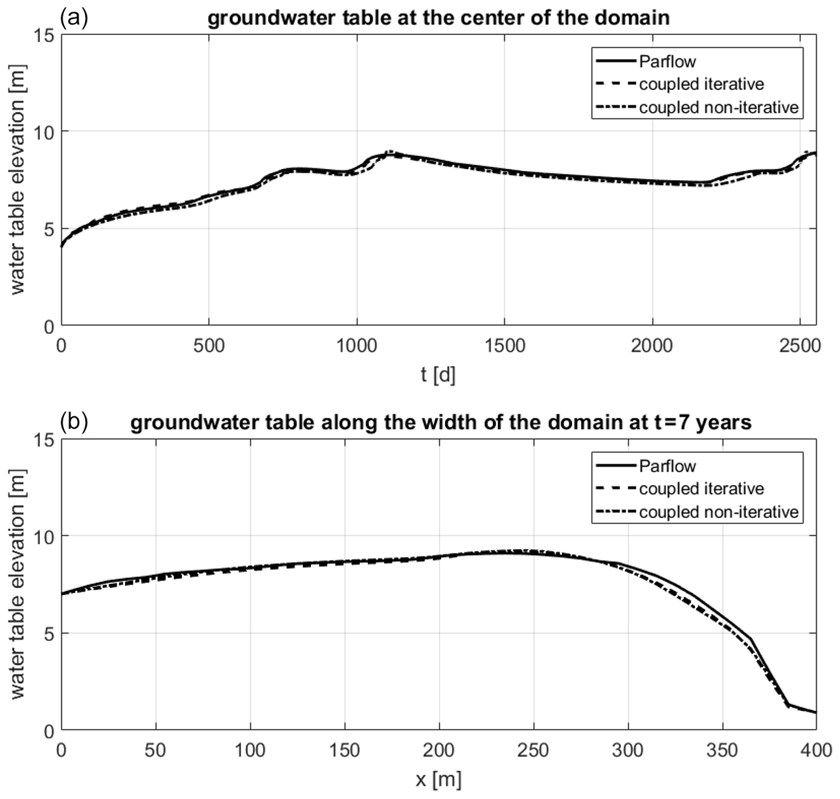
Figure 12 Results of the 3D flow problem. (a) Groundwater table elevation over time in the center of the domain. (b) Groundwater table along the width of the domain (y=400 m) at the final time step.

The heterogeneity of the soil causes more variability of the groundwater table throughout the domain. Figure 13 shows the difference between the groundwater table resulting from the coupled models and the full 3D model at the last time step in the entire domain. It can be seen that in the major part of the domain the differences are small with an average deviation of $\stackrel{\mathrm{‾}}{\mathrm{\Delta }{H}_{\mathrm{GW}}}=\mathrm{0.12}$m for the iterative model and an average deviation of $\stackrel{\mathrm{‾}}{\mathrm{\Delta }{H}_{\mathrm{GW}}}=\mathrm{0.16}$m for the non-iterative model. Areas with larger differences appear at similar locations for both coupling schemes showing the largest deviations close to the lower Dirichlet boundary (between x=300 m and x=400 m). Within these areas the differences between the iterative coupling and the Parflow model are smaller compared to the non-iterative coupling. The reason for these differences can be seen in Fig. 14. The left plot shows the standard deviation of H_GW at the last time step within each zone corresponding to one 1D model obtained with the fully integrated model. The right plot shows the difference to this standard deviation obtained from the iteratively coupled model. It is evident that the variation of H_GW within one zone is much larger between x=300 and x=400 m than in the other parts of the domain. The lumping into zones of equal recharge, specific yield, etc. reduces this variability in the coupled model, leading to larger differences compared to the fully integrated model in these areas. A higher accuracy could be achieved by using more 1D models, but this would also increase the run times.

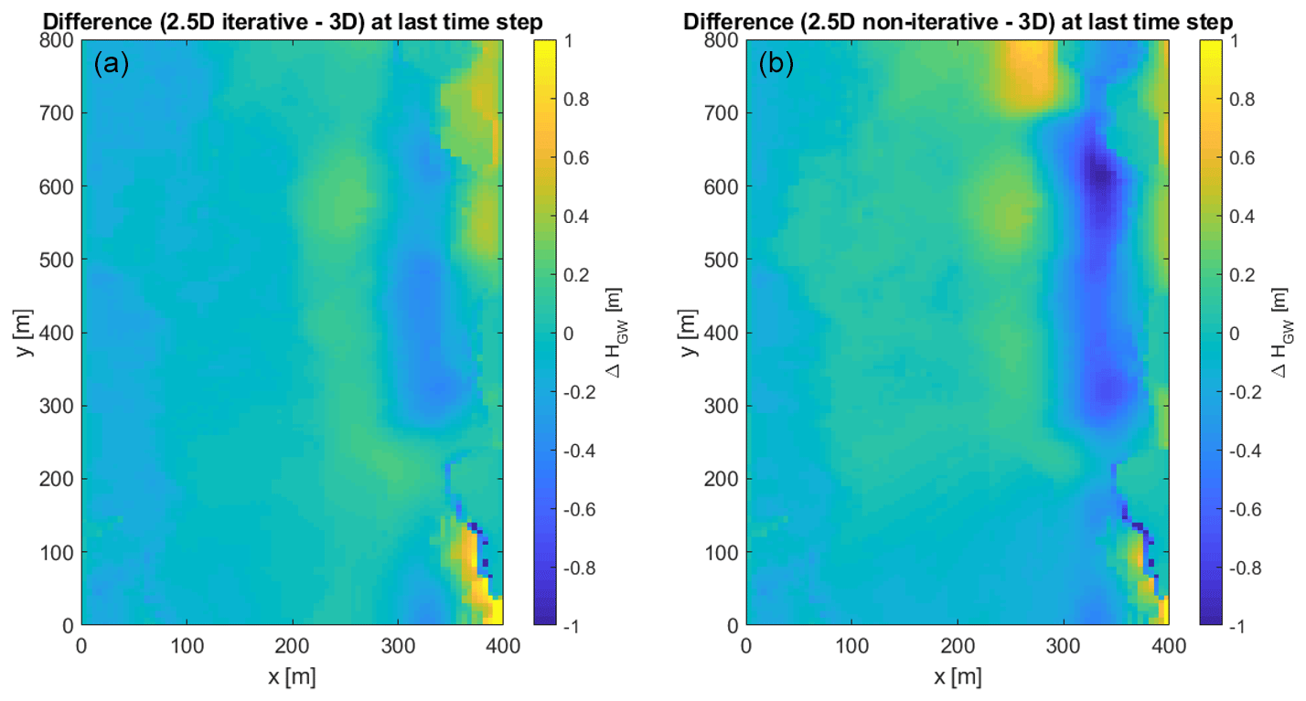
Figure 13 Difference of the groundwater table position compared to the full 3D run at the last time step. (a) Iterative coupling. (b) Non-iterative coupling.

Figure 14 (a) Standard deviation of the groundwater table at the last time step within each zone corresponding to one 1D model in Parflow. (b) Difference of this standard deviation compared to the iteratively coupled model.

The heterogeneity also leads to a larger variability of the specific yield in the iteratively coupled model as can be seen in the left plot of Fig. 15. There is a significant variation in space and time, with values ranging between approximately 0.01 and 0.33. A clear relationship between the groundwater table and the specific yield with an increasing S_y for increasing H_GW, as in the 2D flow case, cannot be seen here. Instead, the soil heterogeneities have a stronger impact on the S_y values. The right plot of Fig. 15 shows the normalized average specific yield and the normalized average saturated hydraulic conductivity at the water table position $K_i=\stackrel{\mathrm{‾}}{K_{\mathrm{s}}\left(H_{\mathrm{GW}}\right)}$. Both lines show a very similar temporal pattern and, except for the time span between t=1400 d and t=2500 d, their values are even close to each other.

Figure 15 (a) Specific yield values resulting from the iterative coupling for the 3D flow problem. The solid line is the spatial average; the dashed lines indicate ±1 standard deviation. (b) Normalized specific yield and saturated hydraulic conductivity at the water table position over time.

For this case, the iteratively coupled model needs roughly twice as much run time as the non-iteratively coupled model (see Table 4). Both coupled models are notably faster than the fully integrated 3D model.

4.4 Results global sensitivity analysis (GSA)

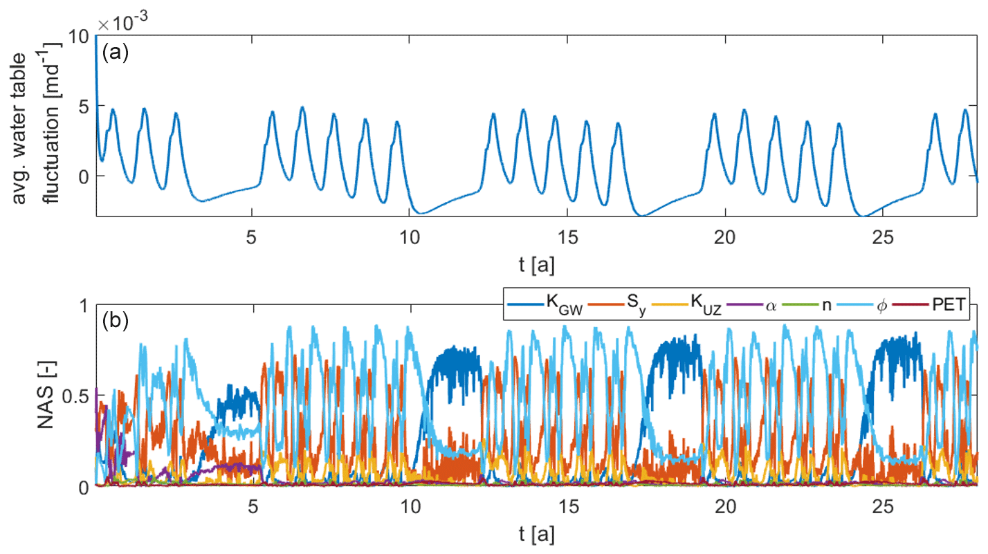
A global sensitivity analysis is performed to identify the most influential parameters of the coupled model regarding the groundwater dynamics, i.e., the groundwater table elevation H_GW and its daily fluctuation ΔH_GW, both taken at the center of the domain. The resulting normalized transient activity score (NAS) data are plotted in the lower plots of Figs. 16 and 17. The upper plots of Figs. 16 and 17 show the water table elevation and fluctuation of the coupled model averaged over all realizations, respectively. Low values of the saturated hydraulic conductivity of the groundwater model K_GW result in a higher curvature of the groundwater table which in some cases reaches the land surface at the center of the domain. All these realizations are removed from the analysis as the model is not able to represent overland flow properly. Therefore, 316 out of initially 500 realizations are used. The polynomial representation (Eq. 16) was cross-validated with 26 randomly chosen parameters and found to be appropriate (result not shown).

Figure 16 shows that the saturated hydraulic conductivity of the groundwater domain K_GW is by far the most influential parameter, except for in the beginning. There, the van Genuchten parameter α is dominant but its influence decreases with time. This is probably due to a spin-up effect. When the model reaches the dynamic steady state (last two cycles), the influence of α has basically vanished. Additionally, porosity ϕ and the specific yield S_y still have a small influence, especially when the water table starts to rise again after a draining period. Note again that the specific yield in the iteratively coupled model is calculated by the model during the simulation. All other parameters play a minor role.

Figure 16 (a) Averaged water table elevation. (b) Transient normalized activity scores.

The activity scores concerning the water table fluctuations look different as can be seen in Fig. 17. Here, the most influential parameters are porosity ϕ, the saturated hydraulic conductivity of the groundwater model K_GW and the specific yield S_y. The dominance of these parameters is alternating. The saturated hydraulic conductivity K_GW is the most important parameter during no-rain periods. The fluctuations are then mainly caused by lateral fluxes, which depend strongly on this parameter. In the iteratively coupled model, when a high or low peak in ΔH_GW is reached, the recharge is the main driving force which is then mostly influenced by porosity. When looking at Eqs. (1) and (7), one sees that S_y can be eliminated when lateral fluxes are negligible compared to the recharge fluxes, which explains why there is no influence of S_y under these conditions. These are the extreme conditions and in between the specific yield has the largest influence. At these times, there is also an increase in the influence of K_UZ. As will be shown later, this is because the calculated specific yield mainly depends on this parameter.

Figure 17 (a) Averaged water table fluctuation. (b) Transient normalized activity scores.

To analyze the sensitivity for different flow conditions, the observations (H_GW and ΔH_GW at the center of the domain) during the last 7-year cycle, when the spin-up is finished, are divided into three categories based on their average groundwater table position during that period: dry (3–7 m), medium (7–11 m) and wet (12–15 m). For each category, the normalized activity scores are calculated and averaged over time. These averaged scores are shown in Fig. 18. The scores shown in Figs. 16 and 17 correspond to the medium case. One can see that, for both the water table position and its daily fluctuation, the sensitivity towards the saturated hydraulic conductivity of the groundwater model is increasing with decreasing depth to groundwater table. Under drier conditions, the influence of porosity and the specific yield is stronger, especially regarding the water table fluctuation. Here, those two parameters become the most influential parameters, while for the water table position the dominance of K_GW remains. The influence of K_UZ on the water table fluctuations is also increasing with increasing depth to water table. Under drier conditions, the unsaturated zone parameters have a stronger impact on the recharge which explains this behavior. Interestingly, there is no increase of sensitivity towards the van Genuchten parameters α and n.

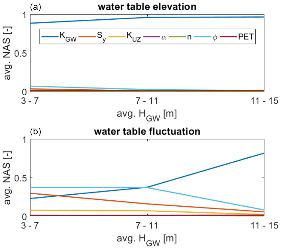
Figure 18 Averaged normalized activity scores of the last 7-year cycle over the average water table position during that period. (a) Normalized activity scores for the water table position H_GW. (b) Normalized activity scores for the water table fluctuation ΔH_GW.

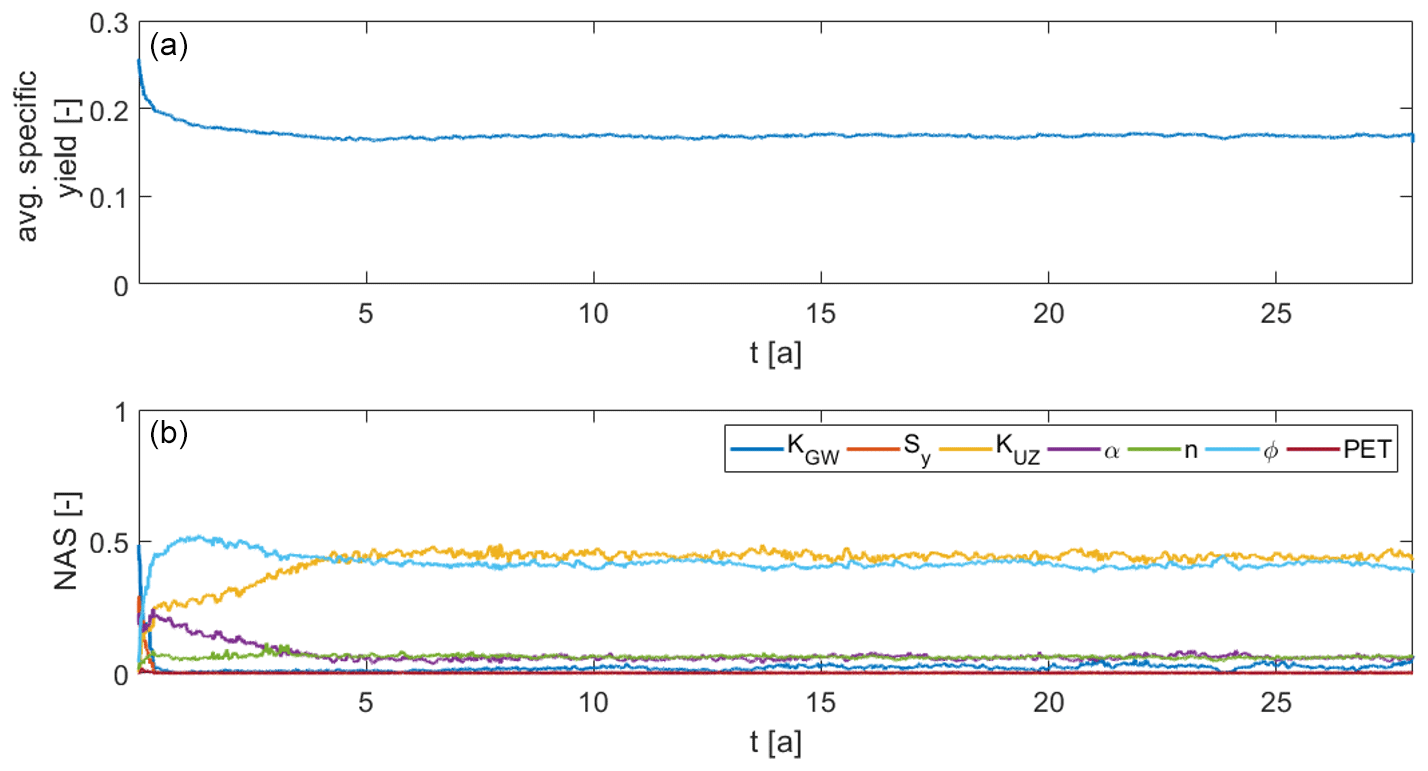
Overall, we see the importance of the specific yield for the groundwater table dynamics. With the iterative calculation of the specific yield, a prior calibration of one of the most influential parameters is not needed. To see whether this calculated parameter behaves reasonably, a sensitivity analysis towards the calculated S_y at the center of the domain was conducted. The results are shown in Fig. 19. Note that the S_y in the parameter list is now an initial value to which no sensitivity is expected. The average calculated S_y value shows some smaller fluctuations, but overall it converges to a value around S_y=0.17, which is a plausible value. The activity scores are also on the whole constant in time with the two most influential parameters being porosity ϕ and the saturated hydraulic conductivity of the unsaturated zone model K_UZ. The strong dependency on K_UZ is consistent with the results of the heterogeneous test case (see Fig. 15). These two parameters are followed by the van Genuchten parameters α and n, whose influence is already much smaller, though. Besides, there is a small influence of the saturated hydraulic conductivity of the groundwater model K_GW. This means that the specific yield is mainly depending on the unsaturated zone parameters. This is reasonable as its intention is to represent the missing unsaturated zone in the groundwater model.

Figure 19 (a) Averaged specific yield values. (b) Transient normalized activity scores.

4.5 Discussion

The above-described numerical experiments show that both coupling methods presented in this work are well suitable to substitute a full 3D model under certain conditions. They can correctly capture the dynamics of the groundwater table in the presence of lateral groundwater flow and soil heterogeneities. The iterative model outperforms the fast but rather approximate non-iterative model in terms of accuracy for all applied test cases, especially in the second one. Its accuracy is comparable to that of other coupling approaches (Beegum et al., 2018), but it is easy to implement and fast, and the model compartments are consistent.

One general problem of the coupled model can be seen in the second test case. Because of the low groundwater table and the large gradient at the lower Dirichlet boundary (x=400 m), water is also leaving the domain laterally via the unsaturated zone. This cannot be captured by the coupled model. The water thus has to first move vertically through the 1D model before it can leave the domain through the groundwater. This leads to a pileup of water and therefore an overestimation of the groundwater table along that boundary. This can also be seen in Beegum et al. (2018), which supports the assumption that it is a general issue. In the 3D flow case (the third test case) the gradient at this boundary is smaller, causing smaller lateral fluxes in the groundwater and thus also in the unsaturated part. Therefore, the results of the coupled model are on average more accurate even though this test case is more complex than the 2D flow case. Here, on the other hand, we see the influence of the simplified recharge and specific yield pattern, which is however unavoidable for the efficiency of the coupled model.

The global sensitivity analysis shows that the groundwater table position H_GW is mainly depending on the saturated hydraulic conductivity in the groundwater model K_GW. This was to be expected as it is the main parameter in the steady-state formulation of Eq. (1). The initially high and then decreasing influence of the van Genuchten parameter α indicates larger fluxes in the unsaturated zone at the beginning of the simulation. This is most likely due to the rather artificial initial condition in the unsaturated zone which enforces unit gradient flow down to 1.25 m above the groundwater table and no flow below. The temporal fluctuations of the groundwater table are influenced by more parameters, namely, the saturated hydraulic conductivity in the groundwater model K_GW, the specific yield S_y and porosity ϕ. Which parameter is dominating depends on the current flow conditions as described in Sect. 4.4.

The dynamic formulation of the specific yield in the iterative coupling approach allows the groundwater model and the unsaturated zone model to respond consistently to the given fluxes. So far this has been a challenge when using an overlapping coupling approach (Zeng et al., 2019). The specific yield values obtained in these experiments confirm the assumption that it is depending on the saturation profile, the fluctuations of the groundwater table and the soil properties. However, these values should be interpreted with some caution. In this model, the specific yield also needs to compensate the influence of the lateral fluxes on the recharge, which cannot be quantified properly. The sensitivity analysis for the parameters’ influence on the calculated specific yield shows that it behaves reasonably, though. It depends on the parameters of the unsaturated zone models, especially on porosity ϕ and the saturated hydraulic conductivity K_UZ. The aim of the specific yield is to represent the missing unsaturated zone in the groundwater model; therefore, a strong dependency on the unsaturated zone model’s parameters is plausible.

5 Conclusions

In this work, two different ways of coupling a 2D groundwater model with multiple 1D unsaturated zone models are presented and compared in terms of accuracy and efficiency. The first approach uses a moving boundary formulation and couples the two domains non-iteratively. In the second approach they are coupled iteratively, and the 1D models overlap with the groundwater model throughout the entire saturated part. A recalculation of the specific yield value during the iteration is applied to get to the same water table position in both model compartments.

The results and run times of the two coupling methods are compared to those of fully integrated model runs. While the iterative coupling shows a higher accuracy, the non-iterative approach is faster. Both coupled models are significantly faster than the fully integrated model. Besides that, the iterative model is more robust, having a decent accuracy for all applied test cases, which is not the case for the non-iterative model, and it can keep the consistency of the two model compartments.

A global sensitivity analysis revealed that the groundwater table position and its dynamics depend mainly on three parameters: the saturated hydraulic conductivity of the groundwater model, the specific yield and porosity. The specific yield is, however, hard to quantify, especially because it is usually not constant over time, and fluctuations can be large in the presence of soil heterogeneities. In the iteratively coupled model the specific yield is calculated by the model itself during the iterations, accounting for this variability. It depends mainly on one additional parameter which is the saturated hydraulic conductivity of the unsaturated zone model. This is an advantage of this method over other existing coupling strategies as this parameter is easier to be quantified and constant over time.

In general, both models qualify for substituting a fully integrated model when computational efficiency is more important than highly accurate results. The iterative approach is more robust and accurate and is recommended for most applications. When speed is essential, the usage of the non-iterative model is also an option. Erdal et al. (2019) used a version of the here-described non-iteratively coupled model successfully to reduce the compute time needed for model spin-up. Another application where such surrogate models can play an important role is data assimilation. Data assimilation often requires an ensemble of model realizations which comes with a strong computational burden. How well the here-presented 2.5D model can replace a fully integrated model in this context is part of ongoing research.