the Creative Commons Attribution 4.0 License.
the Creative Commons Attribution 4.0 License.
 | 06 Jul 2021
Robust historical evapotranspiration trends across climate regimes
Sanaa Hobeichi
Gab Abramowitz
Jason P. Evans
Evapotranspiration (ET) links the hydrological, energy and carbon cycles on the land surface. Quantifying ET and its spatio-temporal changes is also key to understanding climate extremes such as droughts, heatwaves and flooding. Regional ET estimates require reliable observation-based gridded ET datasets, and while many have been developed using physically based, empirically based and hybrid techniques, their efficacy, and particularly the efficacy of their uncertainty estimates, is difficult to verify. In this work, we extend the methodology used in Hobeichi et al. (2018) to derive two new versions of the Derived Optimal Linear Combination Evapotranspiration (DOLCE) product, with observationally constrained spatio-temporally varying uncertainty estimates, higher spatial resolution, more constituent products and extended temporal coverage (1980–2018). After demonstrating the efficacy of these uncertainty estimates with out-of-sample testing, we derive novel ET climatology clusters for the land surface, based on the magnitude and variability of ET at each location on land. The new clusters include three wet and three dry regimes and provide an approximation of Köppen–Geiger climate classes. The verified uncertainty estimates and extended time period then allow us to examine the robustness of historical trends spatially and in each of these six ET climatology clusters. We find that despite robust decreasing ET trends in some regions these do not correlate with behavioural ET clusters. Each cluster, and the majority of the Earth's surface, shows clear robust increases in ET over the recent historical period. The new datasets DOLCE V2.1 and DOLCE V3 can be used for benchmarking global ET estimates and for examining ET trends respectively.
- Article
(6787 KB) - Full-text XML
-
Supplement
(1423 KB) - BibTeX
- EndNote


Understanding the spatio-temporal variability of evapotranspiration (ET) is a critical part of understanding the processes that lead to high impact weather phenomena, such as droughts (Han et al., 2018; Quesada-Montano et al., 2019; Sheffield et al., 2012; Teuling et al., 2013), heatwaves (Teuling, 2018; Ukkola et al., 2018) and flooding (Dawdy et al., 1972; Sharma et al., 2018). Several global gridded ET datasets have been developed, using physical schemes with different scopes (e.g. addressing key questions in ecology, hydrology, or other disciplines) and complexity (see Fisher and Koven, 2020) and empirical techniques including machine learning algorithms, typically incorporating a range of remote sensing inputs (Alemohammad et al., 2017; Jung et al., 2010, 2019). Recently, ET datasets derived with a hybrid approach have been recognised for their potential to outperform single-source datasets in reducing bias against tower-based eddy covariance ET measurements (Ershadi et al., 2014; Feng et al., 2016; Hobeichi et al., 2018; Jiménez et al., 2018; McCabe et al., 2016).
While most observational products are global (or near global) in their spatial extent, and typically available with a monthly time step, different products are constrained by very different types of observations and vary significantly in their treatment of uncertainty. As detailed below when describing the datasets we use here, “physically based” approaches use equations that represent different physical, chemical, and biological processes and incorporate satellite-based atmospheric forcing and parameterisation of land surface characteristics, while “empirical” approaches integrate ground-based measurements of ET together with satellite data and ground-based measurements of vegetation characteristics and land surface parameters. These differences result in a diverse group of products and estimates, but it is their approach to deriving uncertainty estimates that is arguably more important.
Very few datasets provide uncertainty estimates associated with the ET flux; these include datasets described in Bodesheim et al. (2018) and Jung et al. (2019). In Bodesheim et al. (2018), monthly uncertainty estimates are computed from the standard deviation of the half-hourly ET values that were used to derive monthly ET averages. Jung et al. (2019) provide an ensemble of global ET estimates; deviations from the ensemble median are used to derive ET uncertainties. In both cases, uncertainties do not reflect the actual deviation from the measured ET at site locations. Without well-calibrated uncertainty estimates, we are unable to tell whether an identified property of any given dataset, such as a trend or a proportion of the surface energy or water budget, is robust rather than a result of bias or stochastic uncertainty.
ET trends computed from different approaches (i.e. physical and empirical) show general agreement at the global scale, and they indicate that ET has increased since the early 1980s (Miralles et al., 2014; Pan et al., 2020; Zhang et al., 2016). However, different ET products exhibit considerable disparities in regional and continental ET trends. For instance, Miralles et al. (2014) detected upward ET trends in GLEAM (Global Land Evaporation Amsterdam Model; Miralles et al., 2011a, b) in the northern latitudes caused by vegetation greening. In water-limited regions, they found that ET is characterised by a multidecadal variability that follows ENSO (El Niño–Southern Oscillation) dynamics, mainly in eastern and central Australia, southern Africa, and eastern South America. In comparison, ET trends estimated from the observation-driven Penman–Monteith–Leuning (PML; Zhang et al., 2016) model show increasing ET since 1980 in the northern latitudes, arid regions in northern Africa, and northern and eastern Amazon. On the other hand, PML exhibits negative trends in southern South America and western United States. More recently, Pan et al. (2020) found that ET trends exhibited during 1982–2011 by a range of empirical and physically based estimates disagree in the direction of trend in the Amazon basin and many arid and semi-arid regions. Without incorporating uncertainties in ET estimates in the analysis of trends, it becomes difficult to assess the reliability of the established trends.
The gridded ET product derivation technique implemented by Hobeichi et al. (2018) offers the potential for robust out-of-sample testing of its uncertainty estimates, as well as several other advantages over other techniques. Like other merging approaches, it offers the potential to minimise the eccentricities or biases of any one product, by averaging them (in this case using weights). However, unlike several other merging techniques (Mueller et al., 2013; Paca et al., 2019; Rodell et al., 2015; Stephens et al., 2012), it accounts for performance differences between parent estimates using in situ data as the observational constraint rather than assigning weights based on the ability to match another gridded dataset that is deemed more reliable or the ensemble mean of a selection of datasets (Munier et al., 2014; Sahoo et al., 2011; Wan et al., 2015; Zhang et al., 2018). The efficacy of using in situ measurements for constraining much larger-scale gridded estimates has also been shown explicitly (Hobeichi et al., 2018, 2020c). Next, most available merging techniques do not account for dependence between parent estimates, where redundant information in different parent products is likely to bias the hybrid estimate (Abramowitz et al., 2019; Herger et al., 2018). Finally, and perhaps most important for this work, the technique calculates global spatially and temporally varying uncertainty estimates that are based on observations, in that they are based on the discrepancy between the hybrid ET estimate and in situ data. Aside from being more defensible than simply taking the spread of the parent products around their mean (e.g. Pan et al., 2012; Zhang et al., 2018), this approach also allows for out-of-sample testing, by leaving some sites out of the derivation of the hybrid product and its uncertainty and then using them to test its accuracy.
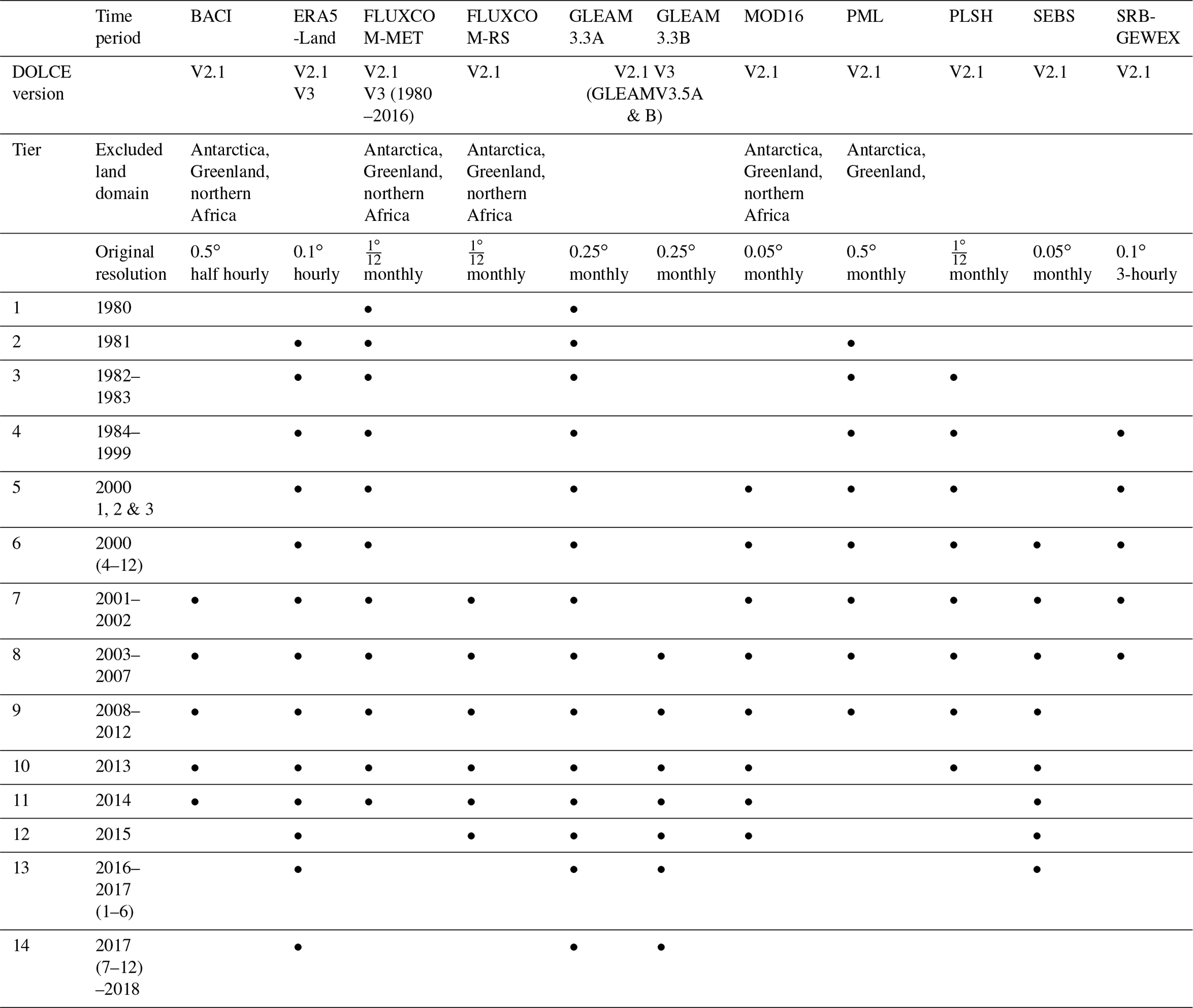
Despite these advantages, out-of-sample testing of uncertainty estimates was not explored by Hobeichi et al. (2018), and the short temporal availability of the DOLCE product (2000–2009) limited its application, particularly in examining historical trends. While different subsets of parent products were used over different regions to expand the spatial coverage of DOLCE, the possibility of different product subsets in different time periods to extend its temporal reach was not explored. Additionally, since the development of DOLCE, four of its six parent datasets (Jung et al., 2010; Martens et al., 2016; Miralles et al., 2011a, b; Mu et al., 2011; Zhang et al., 2016) have been improved, and several new global ET datasets have been developed (Balsamo et al., 2015; Bodesheim et al., 2018; Jung et al., 2019). Most of these are available at a higher spatial resolution than the original 0.5∘ in DOLCE and cover different subsets of the period 1980–2018, with at least two available every year during this period (Table 1).
Table 1Spatial and temporal coverage and original resolution of the global ET datasets (at the time of analysis) used to develop DOLCE V2.1 and DOLCE V3. DOLCE V2.1 was derived from 11 datasets and 14 temporal tiers. DOLCE V3 was derived from four datasets and four temporal tiers, i.e. (1) 1980, (2) 1981–2002, (3) 2003–2016, and (4) 2017–2018.
In this paper we amend these shortcomings and explore some of the insights that the new versions of DOLCE offer, in particular focusing on the temporal trends in ET in different regions and the assessment of robustness of trends that well-calibrated uncertainty estimates afford. Roughly in order, we detail below (1) how we update the DOLCE product with new parent datasets and extend its temporal coverage; (2) how the improved products compare to their previous version and other existing ET estimates from the literature; (3) the efficacy of uncertainty estimates, in particular whether or not they are overconfident; (4) an exploration of historical trends in ET using the extended temporal coverage and how the uncertainty estimates allow us to examine the robustness of these trends; and (5) behavioural ET clusters that describe ET-based climate regimes, as a means to understand the spatial distribution of trends we find.
To derive two new versions of DOLCE, one suitable for benchmarking the ET dataset and another for trends analysis, we combine the 11 and 4 available global gridded ET datasets respectively using the same merging technique as in DOLCE V1. This technique derives a linear combination of the participating ET datasets based on their ability to match in situ observations while also accounting for their error dependency. While we acknowledge the obvious spatial mismatch between gridded and in situ data, we refer readers to Hobeichi et al. (2018) where it was shown that in situ observations do contain useful information about grid-scale fluxes, using out-of-sample testing in a similar framework to the one we present here.
Our aim is to increase the time coverage and spatial resolution of DOLCE V1, as well as examine strategies to improve the effectiveness of the weighting strategy. Below we detail newly available global datasets that allow us to derive DOLCE V2 and DOLCE V3 at 0.25∘ spatial resolution and an improved collection of in situ constraining data. We then briefly revisit the weighting and uncertainty estimation approach before describing our tiering approach to extending the temporal reach of DOLCE V2 and DOLCE V3. Finally, we examine alternative clustering and bias-correction approaches to improve the out-of-sample performance of the weighting technique.
Throughout the paper, we use the two terms evapotranspiration (ET) and latent heat (LE) interchangeably, and the unit watts per square metre (W m−2) for heat fluxes and millimetres per year (mm yr−1) for the water flux equivalent. For reference, 1 W m−2 =12.86 mm yr−1. As above, we refer to the product from Hobeichi et al. (2018) as DOLCE V1 and the new products we are deriving as DOLCE V2 or DOLCE V2.1 and DOLCE V3.
2.1 Data
2.1.1 Global ET datasets
DOLCE V1 was derived from six global ET datasets: MPIBGC (Jung et al., 2010), GLEAM v2a, GLEAM v2b (Miralles et al., 2011a, b), GLEAM v3a (Martens et al., 2016, 2017), MOD16 (Mu et al., 2011) and PML (Zhang et al., 2016). In DOLCE V2, we keep both MOD16 and PML datasets, substitute the GLEAM products with their improved versions GLEAM3.3A and GLEAM3.3B (Martens et al., 2016, 2017), and replace MPIBGC with the newly developed empirical ET datasets from the Max Planck Institute for Biogeochemistry: BACI (Bodesheim et al., 2018) and two ET estimates from the FLUXCOM project (Jung et al., 2019). Additionally, we incorporate a recently published dataset (ERA5-Land; Muñoz Sabater, 2019) and three newly available ET datasets: PLSH (Zhang et al., 2015), SEBS (Chen et al., 2019; Su, 2002) and SRB-GEWEX (Vinukollu et al., 2011). In comparison, DOLCE V3 was derived from four global ET datasets. These are ERA5-Land, an ET dataset from the FLUXCOM project, and the two latest versions of the GLEAM products, GLEAM V3.5A and GLEAM V3.5B. We provide a brief description of these datasets below, with URLs and download dates shown in Table S2.
Biosphere Atmosphere Change Index (BACI; Bodesheim et al., 2018) is derived by upscaling diurnal cycles of ET and other land–atmosphere fluxes from a large set of FLUXNET sites based on a random forest regression framework. It uses seasonal vegetation variables, indices from Moderate Resolution Imaging Spectroradiometer (MODIS) satellites, and meteorological data either measured at the flux tower sites or retrieved from the ERA-Interim data.
ERA5-Land (Muñoz Sabater, 2019) is a global land surface reanalysis dataset that has been developed by rerunning the land component of the ECMWF ERA5 climate reanalysis with a series of improvements (mainly higher temporal frequency and spatial resolution) that makes it more reliable for land applications. ERA5-Land is produced under a single simulation that uses adjusted atmospheric inputs from ERA5 atmospheric variables without being coupled to the atmospheric module of ERA5.
FLUXCOM (Jung et al., 2019) is an empirical upscaling of observations from 224 flux tower sites using machine learning methods. The full FLUXCOM product includes 63 global ET datasets that have been produced using two different setups: a remote sensing (RS) setup and a remote sensing plus meteorological (MET) setup. The development of the global datasets incorporates nine machine learning techniques, four global meteorological datasets (used only with the MET setup), three correction methods for energy imbalance at the flux tower sites and MODIS remote sensing input. In DOLCE V2, we include one dataset from each setup, which we refer to as FLUXCOM-RS (from the RS setup) and FLUXCOM-MET (from the MET setup). To choose the two datasets, we analysed the pair-wise error correlations of all the products against in situ flux tower data and selected the two that had the lowest pair-wise error correlation (and so were deemed least dependent). In DOLCE V3, we include a dataset from the MET setup only.
Process-based Land Surface Evapotranspiration/Heat Fluxes algorithm (PLSH; Zhang et al., 2015) terrestrial ET is derived using an improved Normalized Difference Vegetation Index (NDVI)-based Penman–Monteith algorithm originally developed in Zhang et al. (2010). ET is regulated by a set of geophysical data from GIMMS and Vegetation Index and Phenology along with radiative data from Climate Research Programme/Global Energy and Water Exchanges (WCRP/GEWEX) Surface Radiation Budget (SRB) and CERES along with other meteorological observation data from the NCEP/DOE AMIP-II Reanalysis (NCEP2; Kanamitsu et al., 2002).
In the Surface Energy Balance System (SEBS; Chen et al., 2019; Su, 2002), the ET estimates are produced with the revised Surface Energy Balance System (SEBS) algorithm in Chen et al. (2013, 2019). It uses meteorological observations, ground heat flux, net radiation and canopy measurements collected from flux tower sites, as well as NDVI and emissivity data from MODIS.
In Surface Radiation Budget (SRB)-GEWEX (Vinukollu et al., 2011), ET is estimated based on the Penman–Monteith equation. Input datasets include remote sensing data from Advanced Very High Resolution Radiometer (AVHRR) and MODIS, meteorological data derived from the Variable Infiltration Capacity (VIC; Liang et al., 1994) land surface model forced by Princeton Global Forcing (PGF), and radiative data from the NASA Global Energy and Water Exchanges (GEWEX) Surface Radiation Budget Project (Stackhouse et al., 2011).
It is clear that different parent datasets share forcing, parameterisations, and physical and empirical assumptions. Therefore, they do not constitute entirely independent estimates. Furthermore, their error correlation (when compared with data from 254 sites – details on these below), which can be used as a measure of their dependence (Bishop and Abramowitz, 2013), is high (Fig. S2, correlation >0.5), reinforcing the potential for benefit using a weighting approach that can account for this redundancy.
Part of the high correlation is of course due to spatial heterogeneity and the scale mismatch between in situ and gridded datasets since individual site locations within a grid cell are likely biased with respect to the (unknown) true grid-cell-averaged flux. While it might appear that a weighting approach that accounts for error correlations between parent datasets might be in danger of overfitting to error correlation resulting from spatial heterogeneity, we have two mechanisms that ensure this is not a concern for our final product. First, weights for each product are constructed over very large spatio-temporal domains, i.e. more than 13 000 space-time records as described below, so the (assumed stochastic) biases of individual sites relative to grid cell values are unlikely to influence weights over a large sample. In fact, representativeness of point-scale measurement for the grid scale does exist across all the flux tower sites as a whole; this has been verified by Hobeichi et al. (2018). Second, and more categorical, all results here are presented with out-of-sample testing, so any overfitting will degrade rather than improve the results we present. More detail on this is presented below.
Given that most of the parent datasets provide ET information at a 0.25∘ or finer spatial resolution (Table 1), it is possible to enhance the resolution of DOLCE from 0.5 to 0.25∘. All the parent datasets are resampled from their original spatial resolution to a common 0.25∘ grid using the nearest-neighbour resampling method and aggregated to monthly temporal scale before implementing the weighting technique.
2.1.2 Flux tower data
We use flux tower observations from a range of networks including Ameriflux (https://ameriflux.lbl.gov/, last access: 1 October 2020), the Atmospheric Radiation Measurement (ARM; https://www.arm.gov/, last access: 1 October 2020), AsiaFlux (https://www.asiaflux.net/, last access: 1 October 2020), European Fluxes Database (http://www.europe-fluxdata.eu/, last access: 1 October 2020), Fluxnet 2015 (https://fluxnet.org/data/fluxnet2015-dataset/, last access: 1 October 2020), LaThuile Free Fair Use (https://fluxnet.fluxdata.org, last access: 1 October 2020), Oak Ridge data repository (https://daac.ornl.gov/, last access: 1 October 2020), OzFlux (http://www.ozflux.org.au/, last access: 1 October 2020) and data acquired through communication with individual site principal investigators (PI). Particular efforts were made to establish connections with PIs in regions where ET observations are scarce, including all areas outside North America, Europe and Australia, particularly the MENA (Middle East and North Africa ) region, Siberia, central Africa and the Amazon basin. Our efforts and communications with many PIs unfortunately failed to incorporate flux data from some of these regions (excepting those that are already available from the cited networks). Before the quality control process detailed below, we had obtained data from 366 flux tower sites.
The raw data consist of a composite of half-hourly, daily and monthly records. We compute daily averages from half-hourly records for days when at least 80 % of half-hourly LE records are available. Subsequently, we compute monthly averages from daily records for months when at least 80 % of daily LE records are available. In DOLCE V1 we applied a less strict quality control on the observational data in which up to 50 % of gap filling was allowed. The reason was that DOLCE V1 incorporated much fewer observational data – sourced from Fluxnet 2015 and LaThuile Free Fair use only. In order to retain enough observational data to constrain the weighting, it was necessary to make a trade-off between the quality and the quantity of the data.
We also apply energy balance corrections to the monthly LE at all sites where monthly averages of the other variables of the surface energy budget – net radiation (Rn), ground heat flux (G) and sensible heat flux (H) – are available with the same high quality (quality flag >80 %). Corrections are carried out independently for every monthly record. Where any of the other components of the energy budgets are absent, latent heat measurements are used without any corrections. The energy balance correction is applied as a Bowen ratio (BR)-based correction that distributes the energy budget residuals among H and LE in such a way that their ratio is conserved. This is done under pre-defined constraints that disallow large changes to be applied to LE. As a result of this, we accept the BR correction and use the corrected LE (LEcor) values if the original monthly LE and LEcor satisfy
In DOLCE V1, we did not set a threshold for LE adjustments, which resulted in LE being changed drastically in a few sites to offset errors in the other energy balance components. If the BR correction does not meet the above criterion, we reject the correction and try using a residual correction, which simply calculates LE as the residual term in the energy balance equation; i.e. . Similarly, we reject the residual correction if the relation between LE and LEcor above is not satisfied. In this case, we use the original monthly LE values without correction. A simplified flow chart of these steps is displayed in Fig. S3 in the Supplement. A study by Paca et al. (2019) examined the changes to flux tower LE by three means of correction and found that these on average differ by around 20 W m−2 from one another. On this basis, we expect that, typically, the correction of flux tower LE should not exceed 20 W m−2, unless errors in other components of the budgets are propagating in the corrected ET. The rule for correcting small fluxes and the condition in which each rule is applied (i.e. LE = 30 W m−2) are in part subjective and in another part based on a case-by-case assessment of changes induced on ET by the correction techniques, and they achieve a reasonable trade-off between data quality and availability.
In a further pre-processing step, if a site is located in close proximity to other sites such that they all sit on the same 0.25∘ grid cell, we use observational data from the site that is more representative of the underlying grid cell. Selecting the most representative site among these sites involves (1) identifying the biome cover at each site and (2) computing the fraction of the grid area covered by each biome; the most representative site is the one whose biome is more abundant in the underlying grid cell (i.e. scores the highest fraction of the total area). If all sites are equally representative of the underlying grid cell, we consider them as one site and we combine monthly LE from the sites by taking the average. We use the high-resolution 300 m land cover maps from the European Space Agency (ESA; http://www.esa.int/, last access: 1 October 2020) downloaded from https://cds.climate.copernicus.eu/ (last access: 1 October 2020) to determine the biome types of neighbouring sites and the corresponding grid cells. This step has ensured that we are not matching a grid cell with inappropriate observational data. All the excluded sites are in Europe and North America. This filtering along with the quality control measures described earlier reduced the number of employed sites in this study from 366 sites to 260 sites (Fig. S1). Furthermore, we exclude six sites from the weighting, which were located on flooded land area, wetlands or intensively irrigated land. As a result of this, the constraining observational dataset used to derive DOLCE V2 includes 254 sites with a total of 13 641 monthly records.
2.2 Methods
2.2.1 Weighting approach
The weighting technique is the same as that used in DOLCE V1 and was originally presented by Bishop and Abramowitz (2013) and implemented for merging observational estimates by Hobeichi et al. (2018, 2019, 2020a). It consists of building a linear combination, μ, of the parent datasets that minimises , where represents the monthly time–site records, yj is the observed ET at the jth time–site record. The linear combination is subject to the constraint that , where represents the parent datasets, and is the value of the kth bias-corrected parent dataset (i.e. after subtracting its mean bias relative to the all-site observational dataset) corresponding to the jth time–site record. The analytical solution to this problem accounts for both the performance differences between the parent datasets and their error covariance (Fig. S2), which is a proxy for dependence. Further details on the merging technique can be found in Abramowitz and Bishop (2015) and Bishop and Abramowitz (2013). The weighting approach is used to combine the global parent datasets separately on different spatio-temporal subsets of the entire period and globe, using a tiered approach detailed in Sect. 2.2.3.
2.2.2 Computing uncertainty in ET
The ensemble dependence transformation process developed by Bishop and Abramowitz (2013) is used to calculate the spatio-temporal uncertainty of DOLCE V2 and DOLCE V3. The process transforms the global parent datasets to a new ensemble so that the variance of the transformed ensemble about the derived hybrid ET estimate, μ, is constrained to be equal to the error variance of μ with respect to the flux tower data, averaged over time and space (i.e. across all J records). We use the spread of the transformed ensemble as the spatially and temporally varying estimate of uncertainty standard deviation, which we will refer to as “uncertainty”. We refer the reader to Bishop and Abramowitz (2013) for the derivation of this approach and Hobeichi et al. (2018) for its implementation in this context. The spread of the transformed ensemble accurately reflects the uncertainty of μ in those grid cells where flux tower observations are available. This process ensures that the computed uncertainty provides a better uncertainty estimate of the hybrid ET than simply using the spread of the parent datasets.
One additional advantage of defining uncertainty in this way is that it should give an accurate upper bound estimate of the likely discrepancy between the product and unseen ET measurements at a range of spatial scales. That is, since it is based on the discrepancy of the final hybrid product and point-based flux tower estimates, which are essentially at the extremes of spatial discrepancy, the discrepancy between DOLCE and actual ET at any spatial scale greater than that of a tower footprint and smaller than that of DOLCE should be less than this uncertainty estimate (noting, however, that this is the estimated standard deviation of uncertainty rather than a hard upper limit). In Sect. 2.2.5 below, we detail the out-of-sample testing of this uncertainty estimate at the point scale.
2.2.3 Tiering of dataset subsets in time and space to maximise coverage
To derive DOLCE V1 over the global land, we applied spatial tiering (using different subsets of parent products in different regions to maximise spatial coverage). We now expand this approach to include temporal tiering to improve the temporal reach of DOLCE. Collectively, the incorporated parent datasets have a temporal cover over 1980–2018 but only a short common overlap during 2003–2007 in DOLCE V2 and during 2003–2016 in DOLCE V3, and their spatial intersection does not cover the global land. Therefore, to achieve a global land coverage from 1980 through 2018 without excluding any of their parent products, it was necessary to build DOLCE V2 and DOLCE V3 from different subsets of parent datasets in time periods and land regions depending on the availability of the parent datasets as shown in Table 1. To this end, we consider 14 and 4 distinct temporal tiers in DOLCE V2 and DOLCE V3 respectively. For example, in DOLCE V2, tier 9 covers 2008–2012 and incorporates all datasets except SRB-GEWEX. Tier 1 incorporates the least parent datasets, for the year 1980 (i.e. FLUXCOM-MET and GLEAM3.3A), while tier 8 uses all the parent datasets and covers 2003–2007. Furthermore, within each temporal tier, we consider three spatial sub-tiers, with each spatial sub-tier covering a part of the land. These consist of (a) all land except Antarctica, Greenland and northern Africa; (b) only Antarctica and Greenland; and (c) only northern Africa. A similar spatial tiering approach was also applied in DOLCE V1. Other spatial tiers, each consisting of a small number of grid cells, were also considered where necessary to ensure that no grid cell in DOLCE V2 or DOLCE V3 is missing ET data if a single parent is missing ET data for that grid cell. As a result of the tiering approach, weighting is computed separately using a different subset of parent datasets and site data in each tier, resulting in distinct spatio-temporal subsets of the entire period. Collectively, the hybrid estimates developed throughout the temporal tiers and their spatial sub-tiers form DOLCE V2 and DOLCE V3 over the global land throughout 1980–2018. The reduced number of temporal tiers in DOLCE V3 is to ensure that no temporal discontinuities occur throughout the covered period, which otherwise would have reduced the suitability of DOLCE V3 for trend analysis. In comparison, the incorporation of a larger ensemble of parent products in DOLCE V2 is to derive an optimal ET product that minimises discrepancy with in situ observations.
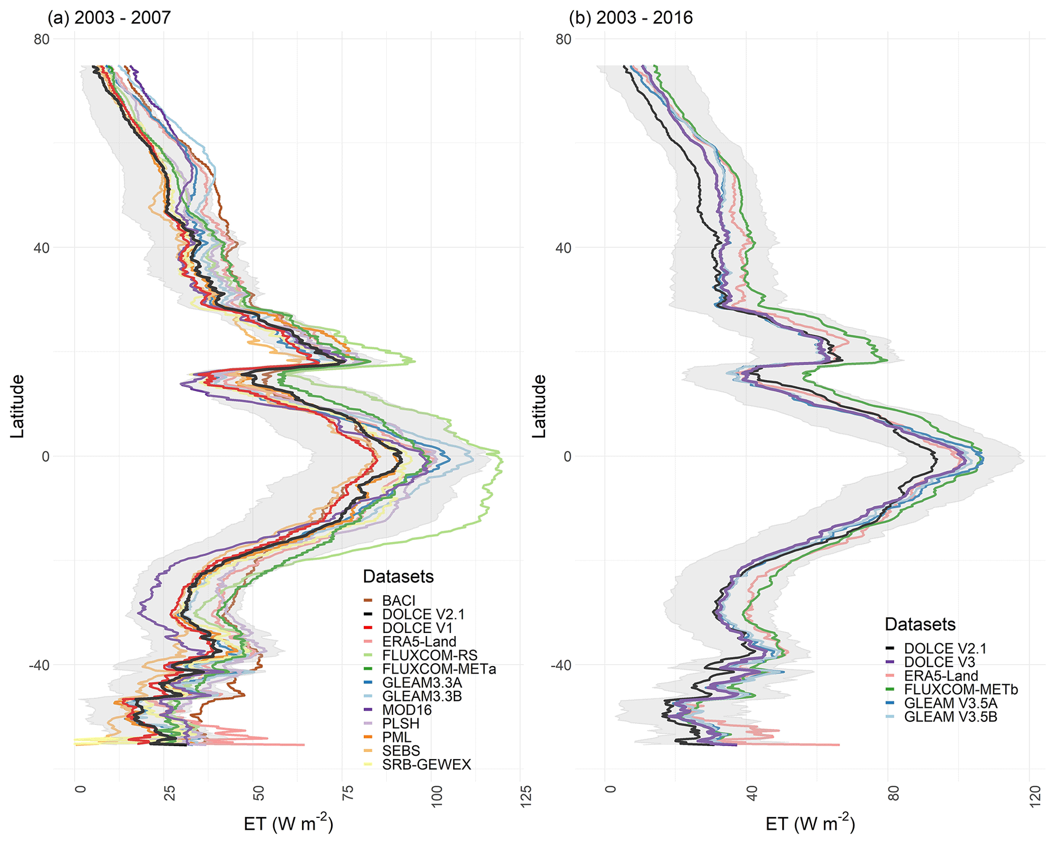
Figure 1(a) Latitudinal means of DOLCE V2 and its parent datasets computed over a common period 2003–2007 and a common spatial mask. (b) Latitudinal means of DOLCE V3 and its parent datasets computed over a common period 2003–2016 and common spatial mask. The grey ribbon represents the values of DOLCE ± uncertainty. DOLCE V1 and DOLCE V2 are included in (a) and (b) respectively for comparison. FLUXCOM-METa and FLUXCOM-METb are two different datasets from the FLUXCOM-MET setup.
2.2.4 Weighting groups
Previous studies have found that the performance of a global product can vary with different climatic circumstances, suggesting that separating the weighting into separate regions or other groupings might well improve the results of the weighting overall (Ershadi et al., 2014; Hobeichi et al., 2018; Michel et al., 2016). Grouped weighting simply involves dividing the time and/or space covered by a particular tier into different subsets or groups (e.g. with different climatic conditions) and then applying the weighting technique separately for each group (within a single tier). We expect that grouped weighting has the potential to improve weighting by accounting for the variation in performance of the parent datasets over different climate or land conditions and can hopefully improve biases detected in DOLCE V1. Hobeichi et al. (2018) tried to group flux tower sites based on their land cover type and computed weights for each land cover type. However, this approach did not improve the results, whether grouping by climate zone or aridity index, with the main reason being attributed to the small number of sites in many groups. Despite the availability of 100 additional sites to constrain the weighting here compared to Hobeichi et al. (2018), the ratio of the observational data to the number of parents has not improved across several climate or land cover types for DOLCE V2. We therefore investigate new approaches to grouped weighting that allow for sufficiently low group numbers to keep a reasonable sample size in each of them, including the following:
-
Grouping by latitudinal zone. This is a simplification of grouping by climate type in which climates are aggregated into three latitudinal zones: (i) high latitudes (±60∘ poleward), (ii) mid-latitudes (±60∘ towards the subtropics ±40∘), and (iii) tropics and subtropics (between −40 and 40∘). In each zone we apply a separate weighting using the corresponding group of sites.
-
Grouping by continents. Sites are naturally separated by continental boundaries, and we might suspect that a particular ET product performs differently across continents. For instance, precipitation is involved in the derivation of many of the parent datasets and has been found to have different fidelity over different continents (Hobeichi et al., 2020b).
-
Grouping by hemisphere. Pan et al. (2020) found that ET estimates agree more in the Northern Hemisphere than in the Southern Hemisphere. Therefore, performing separate weighting in each hemisphere could be better than weighting across all global land.
-
Grouping by seasons. Several studies have shown that the skill of ET datasets varies by seasons (Jiménez et al., 2018; Long et al., 2014; Mueller et al., 2011). To capture these differences, we implement grouping by seasons and grouping by months (detailed below). We consider two combined seasons i.e. summer–autumn and winter–spring. In the summer–autumn season, we constrain the weighting with (1) monthly observations from sites located in the Northern Hemisphere during the period June–November and (2) monthly observations from sites located in the Southern Hemisphere during the period December–May. The remaining observational data are used to constrain the weighting during the winter–spring combined season.
-
Grouping by months. This is similar to grouping by seasons, the only difference is that the two groups are June–November and December–May, without accounting for the different seasonal phase between hemispheres.
-
Grouping by ET regime and months. Land was classified into three distinct, broad ET regimes (Fig. S4) according to two aspects of ET: mean annual total ET and within-year relative variability throughout 1980–2018, derived from GLEAM V3.5A, and using K-means unsupervised classification (MacQueen, 1967). We explain the classification method further in Sect. 3.5.2. Different sets of weights were computed at each ET regime during June–November and December–May. Implementing weighting this way ensured that we account for performance differences across different physical aspects of the land and seasons. Despite the fact that observational data were divided into six distinct groups, the observational data available in each group were still appropriate to merge the four parent datasets of DOLCE V3. However, we found this grouped weighting strategy to be not appropriate for merging 11 parent datasets of DOLCE V2.
As an alternative to the grouping strategies, we also investigate if deriving a spatially varying bias correction within each tier could further improve the weighting. We describe the examined bias-correction approaches and their effectiveness in the Supplement.
2.2.5 Out-of-sample testing approach
To test the effectiveness of different weighting groups or bias-correction approaches, as well as assess which strategy offers the best performance, we use out-of-sample tests. To do this, we first divide the flux tower sites between the in-sample and out-of-sample groups by randomly selecting 25 % of the sites as out of sample. The remaining sites form the in-sample training set are used to compute bias-correction terms and weights for the parent datasets in each tier using the weighting technique without weighting groups (as adopted in DOLCE V1) and with each of the groups and bias-correction strategies detailed in Sects. 2.2.5 and S4 in the Supplement. In each case, these bias-correction terms and weights are then applied to the parent datasets and compared to the out-of-sample sites to test efficacy of the clustering or bias-correction approach employed. The process is repeated for each grouping or bias-correction strategy to derive several hybrid ET datasets for each sample group of sites.
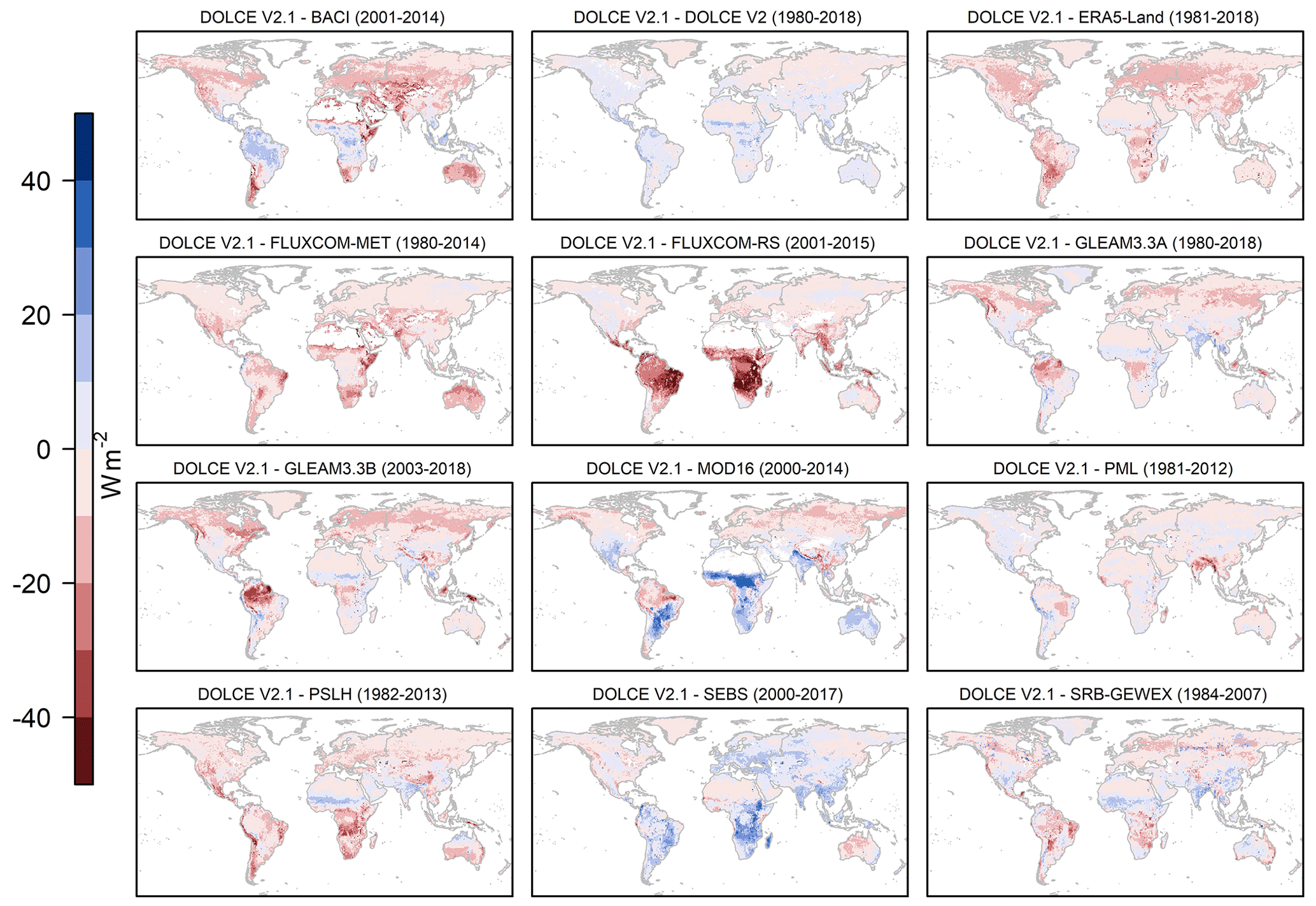
Figure 2Spatial distribution of differences in ET climatology between DOLCE V2 and each of its parent datasets and DOLCE V1. Different spatio-temporal masks are applied for each comparison based on the spatio-temporal coverage of DOLCE V2 and the other datasets.
For each strategy, the test was repeated 1000 times with a different random selection of sites being out of sample. The performance of each hybrid ET estimate was evaluated across five statistical metrics. These were root mean squared error (RMSE), absolute standard deviation difference (), correlation, mean absolute deviation (i.e. mean()) and median absolute deviation (i.e. median()). DOLCE V1 has not been included in this test as its coarser spatial resolution (i.e. 0.5∘) excludes many coastal sites and so significantly reduces the observational data we could use in this analysis. The out-of-sample test is carried out over the common period of availability of all the parent datasets, i.e. 2003–2007 and 2003–2016, to enable comparison of the out-of-sample performance of each approach with all of the 11 and 4 parent datasets of DOLCE V2 and DOLCE V3 respectively.
We perform another out-of-sample experiment to test if the uncertainty estimate derived by the successful grouping and/or bias-correction strategy performs well out of sample. In this test, we first select a site S, but instead of constraining the weighting using observed ET from this site, we compute the weights and bias-correction terms of the parent datasets by using all the sites except S (i.e. just one site is out of sample). We then calculate the mean squared error (MSE) of the derived hybrid ET against observations from all the sites except S. We denote this value by uncertaintyin-sample, since it represents the uncertainty estimate computed using the same observational dataset that we used to train the weighting. We also calculate the MSE of the hybrid ET against the out-of-sample observations from S, and we denote this as uncertaintyout-sample, since we perform the comparison against ET observations that have not been used to train the weighting. We repeat this test for all the sites, and each time we calculate the ratio . In an ideal case, this ratio should equal to unity.
3.1 Out-of-sample performance of DOLCE V2 and DOLCE V3
We derive DOLCE V2.1 (Hobeichi et al., 2020b) from 11 parent datasets by applying a grouped weighting by months. As detailed in the Supplement (Sect. S5), this approach achieves slightly better out-of-sample performance than the other grouped weighting approaches in estimating ET (Fig. S6) and in deriving more robust uncertainty estimates (Fig. S7). We recall that in grouped weighting by months, the observational and gridded ET data are split into two groups: one covering the period June–November and the other covering December–May. Weighting and bias correction is then implemented in each group separately for each tier to create the subsets from which the hybrid ET product is derived.
We derive DOLCE V3 (Hobeichi et al., 2021) from four parent datasets by applying a grouped weighting by ET regimes and months. Both DOLCE V3 and DOLCE V2.1 outperform their parent datasets in the out-of-sample tests across all performance metrics (Figs. S6 and S8). DOLCE V2.1 performs better than DOLCE V3 across all performance metrics except standard deviation difference as illustrated in Fig. S8. The overall better performance of DOLCE V2.1 is expected given that more ET estimates contribute to the weighting. On the other hand, DOLCE V2.1 has proven worse performance than DOLCE V3 in capturing variation in ET observations since variability in ET should have decreased when the variations in individual products are not temporally coincident.
3.2 Comparison of DOLCE V2 and DOLCE V3 with their parent datasets
Figure 1 displays the latitudinal means of each of DOLCE V2 and DOLCE V3 and their parent datasets computed over a common spatial mask and common periods of 2003–2007 and 2003–2016 in the case of DOLCE V2 and DOLCE V3 respectively. The grey ribbon represents the uncertainty of DOLCE V2 and DOLCE V3 in Fig. 1a and b respectively, defined by the ± uncertainty standard deviation interval. The uncertainty standard deviation of the two DOLCE products mostly contain the latitudinal variations of their parent datasets with the exception of FLUXCOM-RS, which exhibits larger ET over the tropics and subtropics of the Southern Hemisphere relative to DOLCE V2 (Fig. 1b). This containment should not be surprising since uncertainty estimates should be robust for point-scale estimates. Figure 1a shows that DOLCE V1 exhibits a slightly lower ET than DOLCE V2 in the tropics and subtropics. DOLCE V2 appears in the lower end of the range of the other datasets from 60∘ poleward. All the datasets exhibit considerable disparities over the mid-latitudes south of −50∘, where the contribution of the terrestrial ET comes mostly from the lower Andes. The difference between DOLCE V2 and DOLCE V3 is smallest over the mid-latitudes of the Northern Hemisphere where most of the flux tower sites are located and is largest over the tropics where very few observations are available. Also, both the number and the spread of parent datasets are larger in DOLCE V2, which explains its larger uncertainty compared to DOLCE V3. The parent datasets of DOLCE V3 are in general in the upper range of ET across all the different participating products, which also explains why DOLCE V3 exhibits larger ET than DOLCE V2 throughout the land and mostly over the tropics.
Figure 2 shows the spatial distribution of differences in the ET mean between DOLCE V2 and each of its parent datasets. We apply different spatio-temporal masks for each comparison based on parent dataset coverage (Table 1). We also compute the climatological difference of DOLCE V2 with its predecessor DOLCE V1 over 2000–2009. A similar plot showing the spatial distribution of differences in the ET mean between DOLCE V3 and each of its parent datasets is provided in Fig. S9. Figure S9 shows that DOLCE V3 exhibits higher ET than DOLCE V2.1 and DOLCE V1 over most of the land, particularly over the tropics and the high latitudes. On the other hand, the climatological difference between DOLCE V3 and its parent datasets show different spatial patterns, and the least climatological difference is between DOLCE V3 and GLEAM V3.5B.
Table 2Mean annual ET aggregates in millimetres per year (mm yr−1) across 20 river basins calculated for DOLCE V2, DOLCE V3 and CDR-ET (Table 4 of Zhang et al., 2018) over a common period 1984–2010. CDR-ET is derived by merging 10 available ET datasets into a hybrid ET which then receives corrections, so the surface water budget established by derived hybrid estimates of the other hydrological variables is closed.
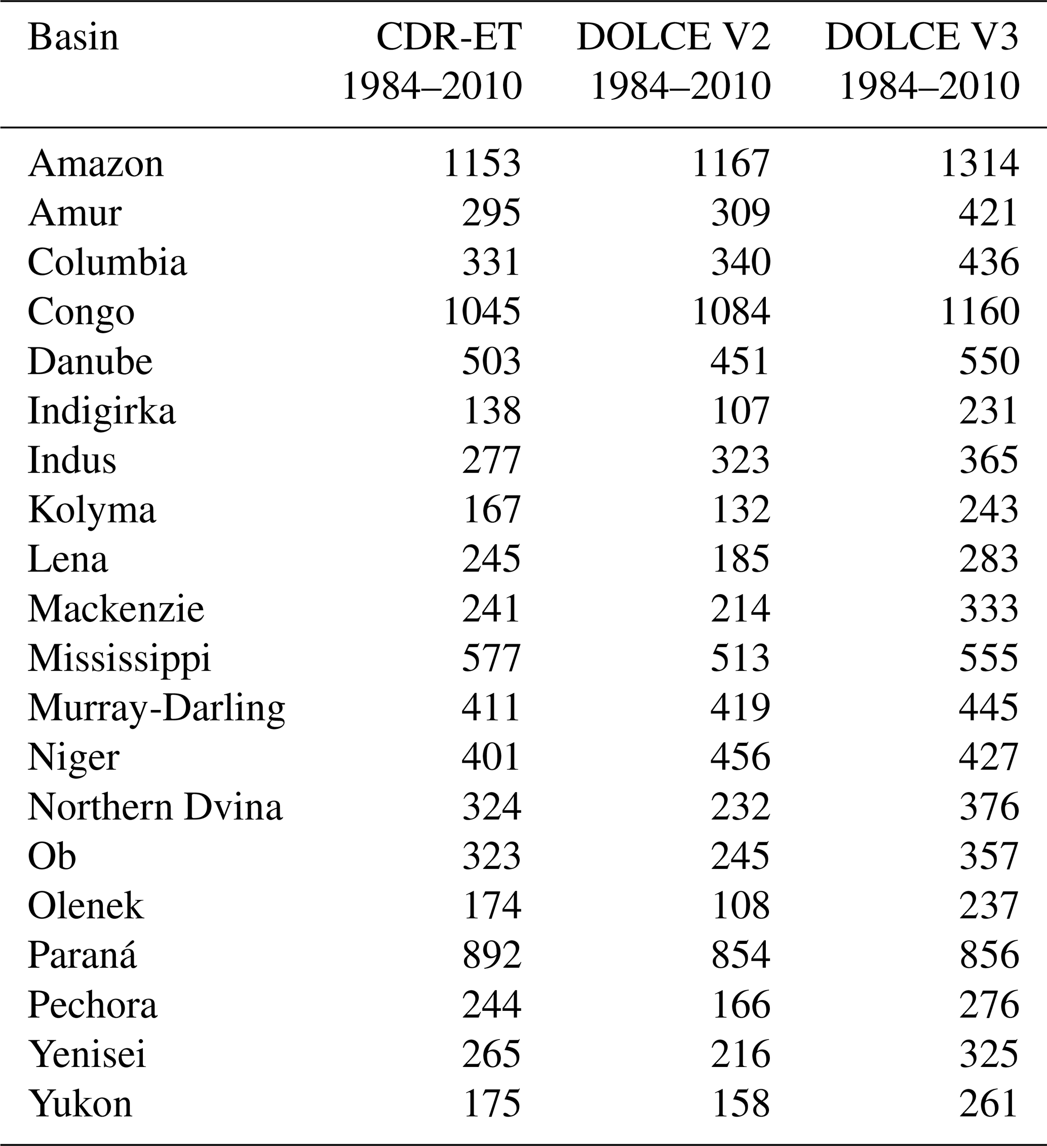
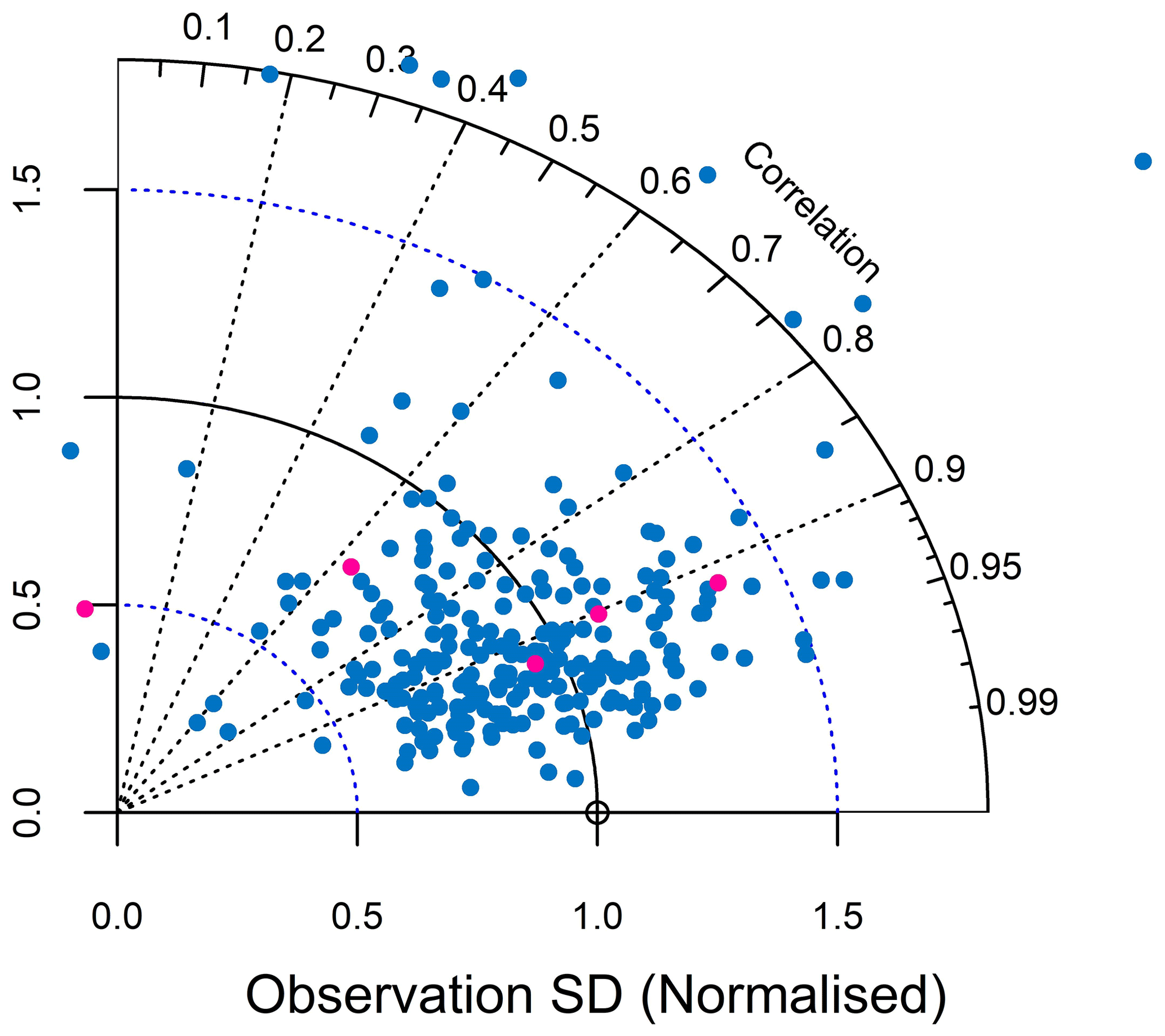
Figure 3Taylor diagram displaying two performance metrics, i.e. correlation and standard deviation of DOLCE V2 relative to normalised observational data presented by a hollow point (reference point) at one unit on the x axis. Pink points represent performance statistics scored at sites located on wetlands, flooded plain or intensively irrigated areas.
Table 3Annual continental averages of ET (W m−2) and its standard deviation uncertainty calculated for DOLCE V2, DOLCE V3 and that developed in L'Ecuyer et al. (2015) over a common period 2000–2009. In L'Ecuyer et al. (2015), ET is derived by merging three global datasets and then adjusted by enforcing the physical constraints of the surface and atmospheric water and energy budgets.
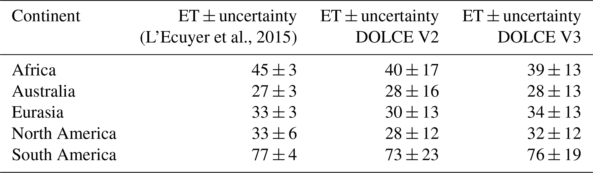
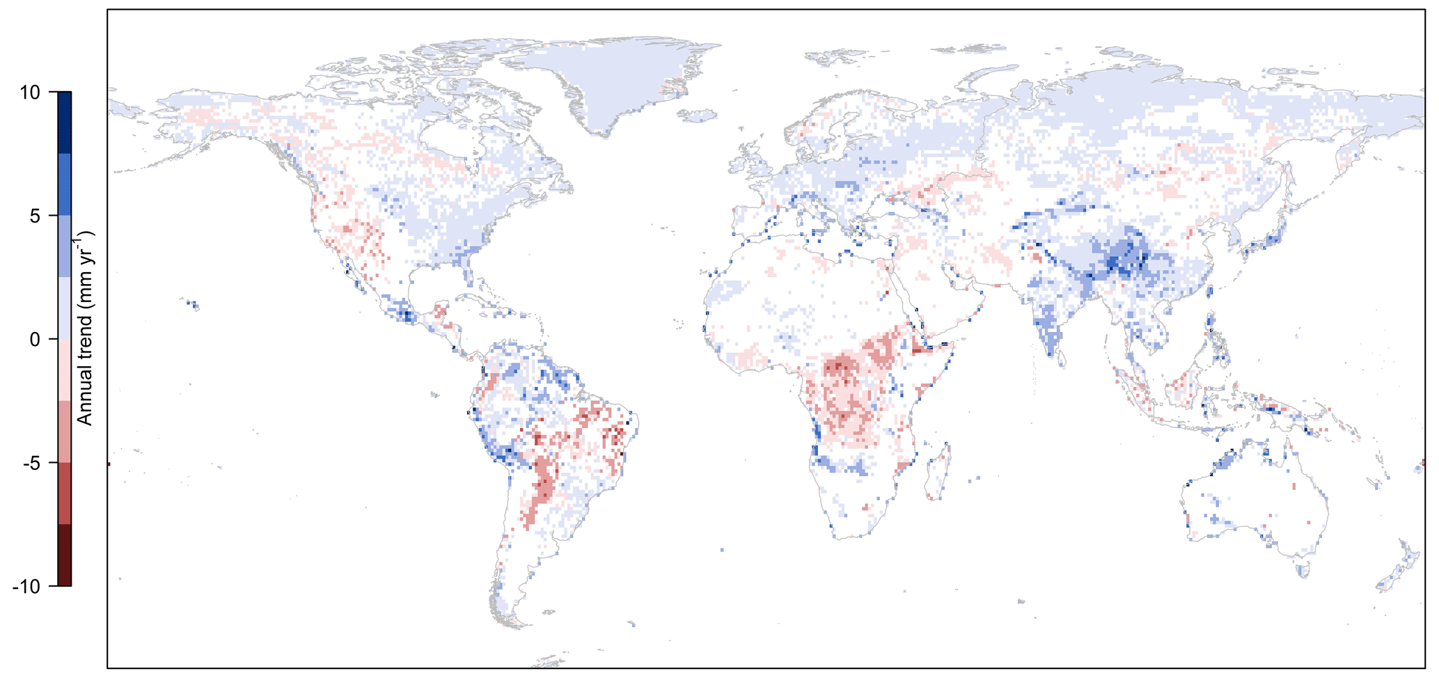
Figure 4Spatial pattern of ET climate trends in DOLCE V3 over 1980–2018 derived using Mann–Kendall and Sen's slope methods. Grid cells in white correspond to unreliable ET trends either because (i) the confidence interval of the slope encompasses a mix of negative and positive values or (ii) trend slopes computed for multiple, different random samples of ET within the interval ET ± uncertainty do not agree in sign.
Over the temperate regions of the Northern Hemisphere, DOLCE V2 exhibits lower mean ET than all its parents except SEBS. We have computed the mean bias of all these datasets relative to the observational data available from sites located in these temperate latitudes. DOLCE V2 has a negligible bias of 0.2 W m−2 relative to the observational data. This bias results from a positive bias of 0.4 W m−2 during June–November and a negative bias of −0.2 W m−2 during December–May. All the parent datasets except SEBS exhibit a positive bias that ranges between 2.7 and 11.4 W m−2, and SEBS has a negative mean bias of −3.4 W m−2 that varies between −0.2 W m−2 during December–May and −6.3 W m−2 during June–November. We note that the bias relative to the in situ observational datasets is only indicative of the performance of the gridded datasets at the sites and does not necessarily represent the actual mean bias over these regions. The discrepancy between DOLCE V2 and DOLCE V1 is relatively small across all land.
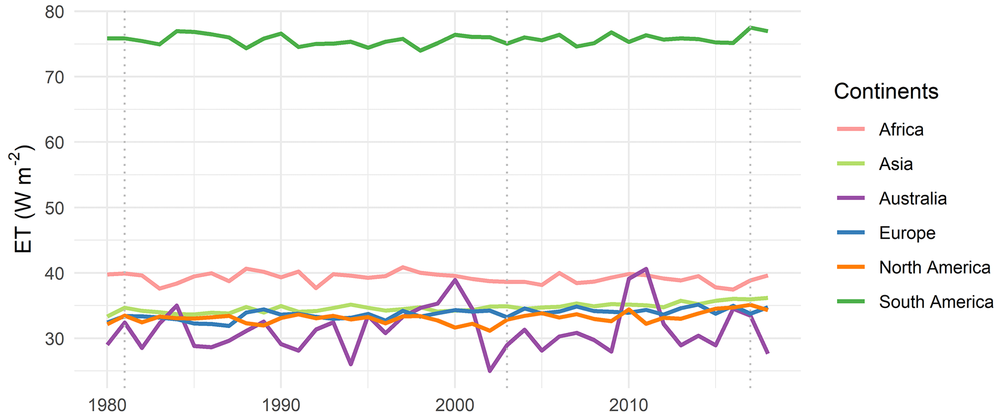
Figure 5Annual average line plots of the area-weighted mean of continental ET exhibited by DOLCE V3. The vertical dashed lines mark the beginning of a new tier in 1981, 2003 and 2017.
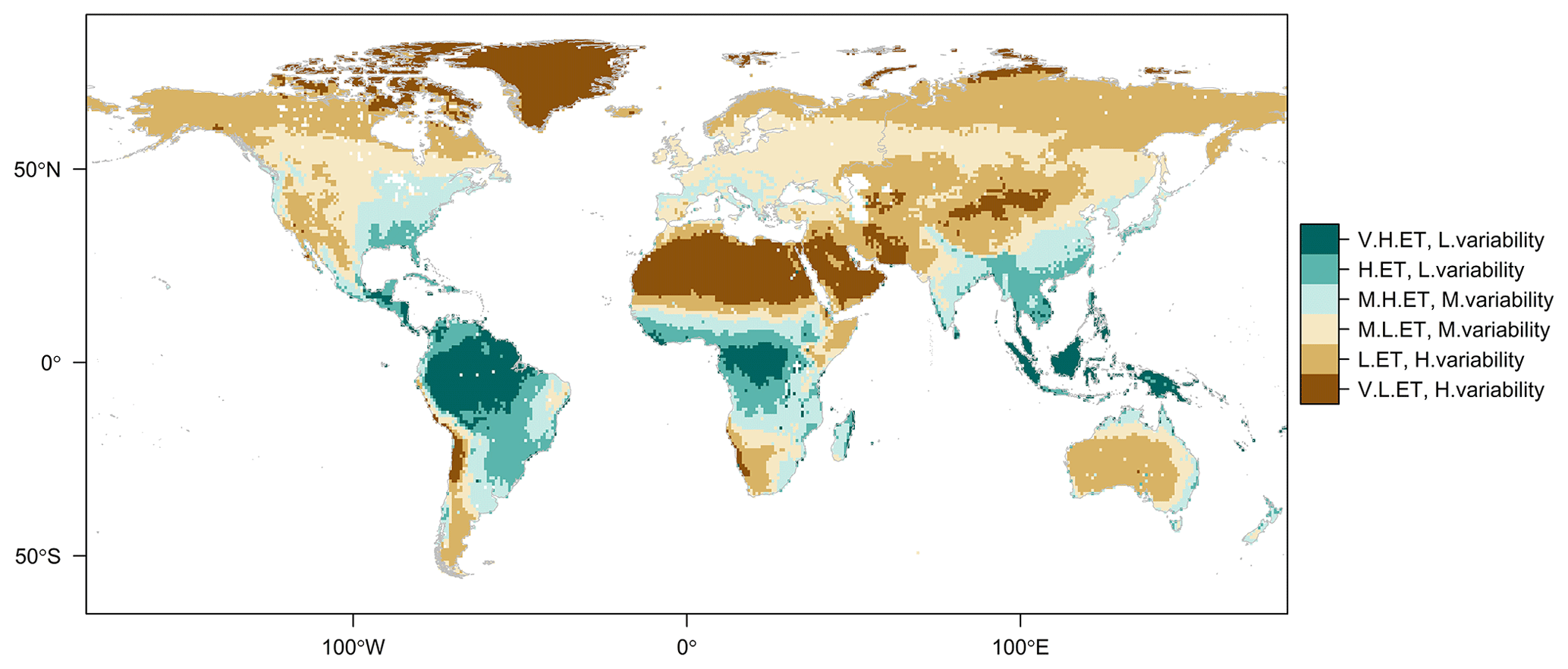
Figure 6Classification of the land into six distinct dry and wet ET regimes using K-means unsupervised classification based on DOLCE V3 annual ET mean and within-year relative variability both computed for 1980–2018. The six ET regimes are labelled from driest to wettest as very low ET with high variability (V.L.ET, H.variability), (ii) low ET with high variability (L.ET, H.variability), (iii) mild low ET with medium variability (M.L.ET, M.variability), (iv) mild high ET with medium variability (M.H.ET, M.variability), (v) high ET with low variability (H.ET, L.variability) and (vi) very high ET with low variability (V.H.ET, L.variability).
Large differences between DOLCE V2 and FLUXCOM-RS are seen over the Congo and the Amazon basins, southern Africa, and the Brazilian highlands. The mean climatological bias of FLUXCOM-RS relative to observational data from these regions is 30 W m−2. This large bias likely results from the lack of sufficient data available to train the machine learning algorithm over climatically distinct biomes, which made ET prediction less constrained. This bias did not appear in FLUXCOM-MET, possibly because ET prediction is based on a larger set of predictor variables. DOLCE V2 exhibits a relatively small bias ranging between 2.6 W m−2 during June–November and 6.4 W m−2 during December–May. In comparison, DOLCE V3 exhibits no significant bias during June–November and a bias of 12.2 W m−2 during December–May, which is similar to the bias in GLEAM V3.5B over these latitudes and seasons and is less than the bias in the remaining parent datasets (i.e. GLEAM V3.5A, FLUXCOM-MET and ERA5.
In general, there are apparent disparities in the patterns of climatological differences in the tropics across all the maps. This results from the fact that global ET datasets exhibit large differences over the tropics, which has been highlighted previously (Paca et al., 2019; Pan et al., 2020), particularly over the Amazon basin.
3.3 Comparison of basin and continental ET with existing literature
We now compare DOLCE V2 and DOLCE V3 with annual mean ET aggregates over a range of river basins documented in a recent study (Table 4 of Zhang et al., 2018). ET in that study – which we'll refer to as CDR-ET – is derived by merging 10 available ET datasets into a hybrid ET which then receives corrections, so the surface water budget – established by derived hybrid estimates of the other hydrological variables – is closed. Table 2 displays the mean annual ET aggregates in millimetres per year (mm yr−1) across 20 river basins calculated for DOLCE V2, DOLCE V3 and CDR-ET over the common period 1984–2010. Our results show that there is an overall agreement between DOLCE V2 and CDR-ET across all the non-Siberian rivers where the difference in ET estimates is mostly around 10 %. The agreement worsens over the Arctic basins Indigirka, Kolyma, Lena, Northern Dvina, Yenisei and particularly over Olenek and Pechora where the differences in ET estimates exceed 20 %. Previous studies have reported large uncertainties in the water fluxes over the Siberian basins (Lorenz et al., 2015), most likely due to the absence of a proper representation of snow and permafrost dynamics (Candogan Yossef et al., 2012). Interestingly, over the North American Arctic basins Mackenzie and Yukon, DOLCE V2 and CDR-ET exhibit much smaller relative differences than at their Siberian counterparts. DOLCE V3 exhibits higher ET than DOLCE V2 and CDR-ET across the majority of the river basins, particularly over the Arctic basins. DOLCE V3 is within the range of its recently developed parent datasets which exhibit higher ET than the older-generation products such as SRB-GEWEX and SEBS incorporated in DOLCE V2.
We also compare DOLCE V2 and DOLCE V3 with continental annual means of ET shown by L'Ecuyer et al. (2015). In their study, they derive a hybrid ET by merging three global datasets. Then, they adjust the hybrid ET and its associated uncertainty by enforcing the physical constraints of the surface and atmospheric water and energy budgets using a data assimilation technique (DAT). Our results show that DOLCE V2 has smaller ET with larger associated uncertainties compared to those derived in L'Ecuyer et al. (2015) (Table 3). The range of their ET estimate overlaps with the range of DOLCE V2 and DOLCE V3 throughout all continents. In L'Ecuyer et al. (2015), the uncertainty estimates are originally taken from the literature and are deemed constant across time and space and then these are reduced by the DAT. The uncertainty estimate of DOLCE, however, is firmly grounded in the discrepancy between the gridded DOLCE product and in situ tower data. The variance of this discrepancy is used to recalibrate the variance of the parent datasets, which are then used to estimate uncertainty, allowing for a spatio-temporally varying uncertainty estimate that is both consistent with the discrepancy between DOLCE and surface observations while at the same time being spatially and temporally complete. This process is detailed by Hobeichi et al. (2018).
Finally, we compare DOLCE V2 with the ET component of Conserving Land Atmosphere Synthesis Suite (CLASS; Hobeichi, 2019; Hobeichi et al., 2020a), which we denote as CLASS-ET. The CLASS dataset comprises coherent estimates of the surface water and energy budgets at the gridded monthly scale. CLASS-ET has been derived by adjusting DOLCE V1 by enforcing the simultaneous closure of the surface water and energy budgets using the same DAT as in L'Ecuyer et al. (2015) and can be therefore considered an improved version of DOLCE V1. Table S3 displays the continental area-weighted averages of DOLCE V2, DOLCE V1 and CLASS-ET and the mean differences DOLCE V2 minus DOLCE V1 and DOLCE V2 minus CLASS computed over a common time period 2003–2009 and using a common spatial mask. We find that, in general, DOLCE-V2 is closer to CLASS-ET (i.e. the improved version of DOLCE V1) than DOLCE V1.
3.4 Performance of DOLCE V2 at flux sites
We now compare DOLCE V2 with ET measured at the 260 sites used in this study (Table S1). We display two performance metrics – correlation and standard deviation – on a Taylor diagram (Fig. 3). All data have been normalised before computing the statistical metrics so that the observational data at each site have a mean of 0 and a standard deviation of 1. Each coloured point summarises the performance statistics of DOLCE V2 at a single site. The observational data are represented by a single “reference” point, i.e. the hollow point at 1 on the horizontal axis. The plot in Fig. 3 shows that most of the coloured points lie close to the reference point, indicating that DOLCE V2 is highly correlated with most of the observational data. Overall, Fig. 3 shows good agreement with the observational datasets. Poor performance is seen over a small number of sites. These are represented by points located outside the Taylor diagram area. Most of these sites have less than 1 year of monthly records with several gaps, perhaps raising questions about observational quality.
In a further analysis, we investigate whether the performance of DOLCE V2 is reduced over a particular land cover type. For this purpose, we repeat Fig. 3, but this time we colour-code the statistics points by the land cover type of the sites they represent as shown in Fig. S10. The new plot does not reveal clear links between the performance of DOLCE V2 and the biome types of the sites. Similarly, we could not find performance links with the degree of representativeness of the site to the underlying grid cell. This is shown in Fig. S11 where colours represent the degree of agreement between the land cover type at the footprint of the tower site and the dominant land cover of the grid cell containing the site. As shown in Fig. S11, we carry out this analysis on the basis of three levels of agreement. These include blue points, representing sites whose land types match the dominant land types of the underlying grid cells; green points, representing sites whose land types cover more than 25 % of the underlying grid cells without being the dominant land cover at these grid cells; and pink points, representing sites whose land types cover less than 25 % of the underlying grid cells.
3.5 Changes in ET since 1980
3.5.1 Annual ET trends over the global land
We use DOLCE V3 to produce a long-term (1980–2018) map of trends in annual ET totals (Fig. 4) as proposed by Mann–Kendall (Kendall, 1948; Mann, 1945) using Sen's slope method (Sen, 1968). We use the uncertainty estimates associated with the ET fields and the confidence interval of the slope as two confidence measures to filter out spurious trends. These confidence measures consider trend behaviours as reliable only if (i) the confidence interval of the slope does not encompasses a mix of negative and positive values and (ii) trend slopes computed for multiple different random samples of ET within the interval ET ± uncertainty standard deviation agree in sign at least 90 % of the time.
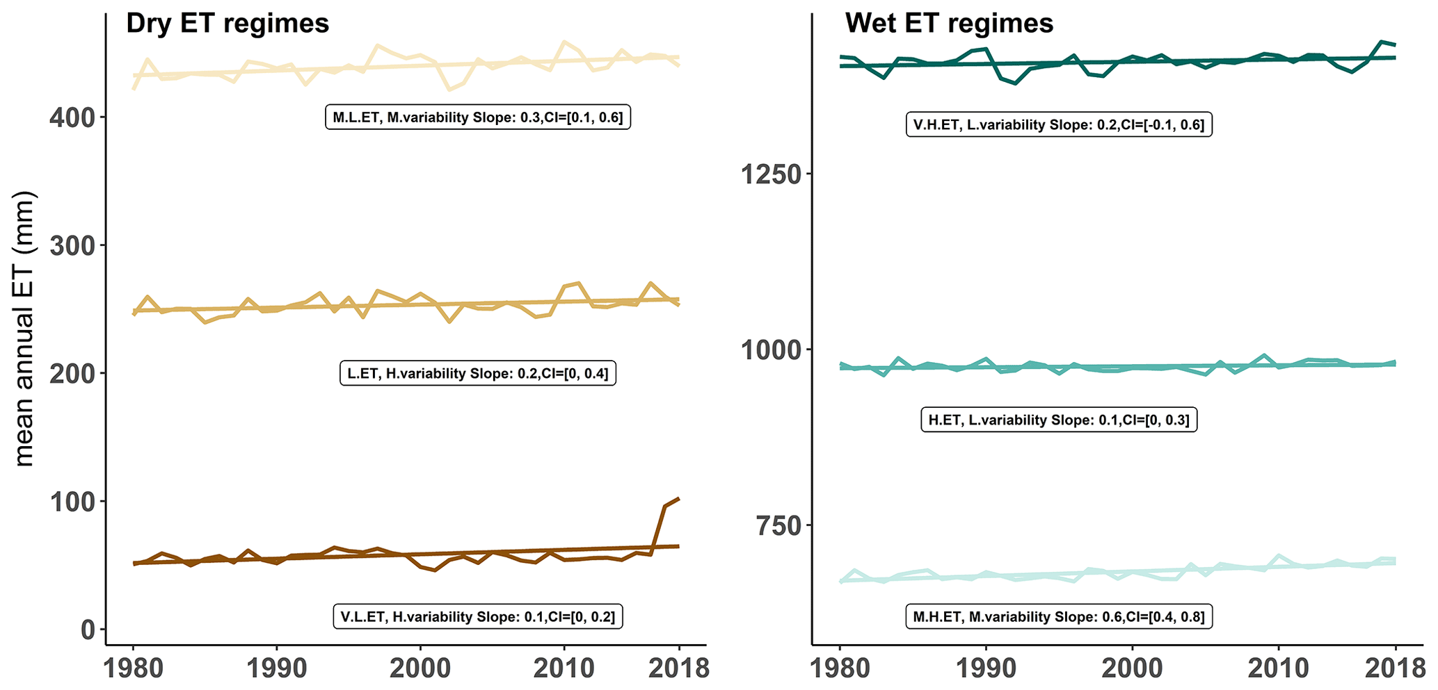
Figure 7Trends in mean annual ET total computed for the dry and wet ET regimes during 1980–2018. Slopes and confidence intervals are computed using Mann–Kendall and Sen's slope methods. The spatial distribution of the ET regimes is illustrated in Fig. 6.
Unreliable trends occur in regions where ET uncertainty is relatively high, such as in northern Africa and the Sahel, and in the high latitudes where ET observations are sparse or do not exist. Inconsistent trend behaviour (confidence interval (CI) includes positive and negative values) is found in regions that experienced long phases of droughts and non-droughts during 1980–2018, mainly in Australia, or a succession of drought and wet events, mainly in southern United States and the Amazon basin (Marengo et al., 2018). As a result of this, a general long trend in ET is not identified in these regions. Miralles et al. (2014) report that these changes in ET over these regions reflect an El-Niño–La-Niña cycle. Similarly, we have not detected clear long trends in southern South America and eastern and southern Africa. This partially agrees with the study of Pan et al. (2020) where their Fig. 8 shows no ET trend in eastern Africa, and no agreement on the sign of trend between the participating datasets has been found in southern South America. Figure 4 indicates that ET has increased over most of the northern latitudes which has been highlighted in many studies (e.g. Miralles et al., 2014; Pan et al., 2020; Zhang et al., 2016), and declined in western United States, central Africa and South America. Unfortunately, given the absence of adequate in situ observations that cover a long enough period to establish trends analysis, it is difficult to validate the identified trends directly.
In further analysis, we verify that the spatio-temporal tiering adopted in DOLCE V3 has not resulted in temporal discontinuities. Figure 5 illustrates the annual average line plot of the area-weighted mean of continental ET exhibited by DOLCE V3. The vertical dashed lines mark the beginning of a new tier, i.e. in 1981, 2003 and 2017. While the line plot does show some marked changes, these do not coincide with changes in tiers and rather coincide with extreme events and are specific to the continents where these events occurred. For instance, in Australia, ET shows high mean annual total in three very wet years (2000, 2010 and 2011) and low levels throughout 2001–2009 during the millennium drought. Additionally, the decline in ET since 2017 is caused by severe droughts that developed across most of Australia.
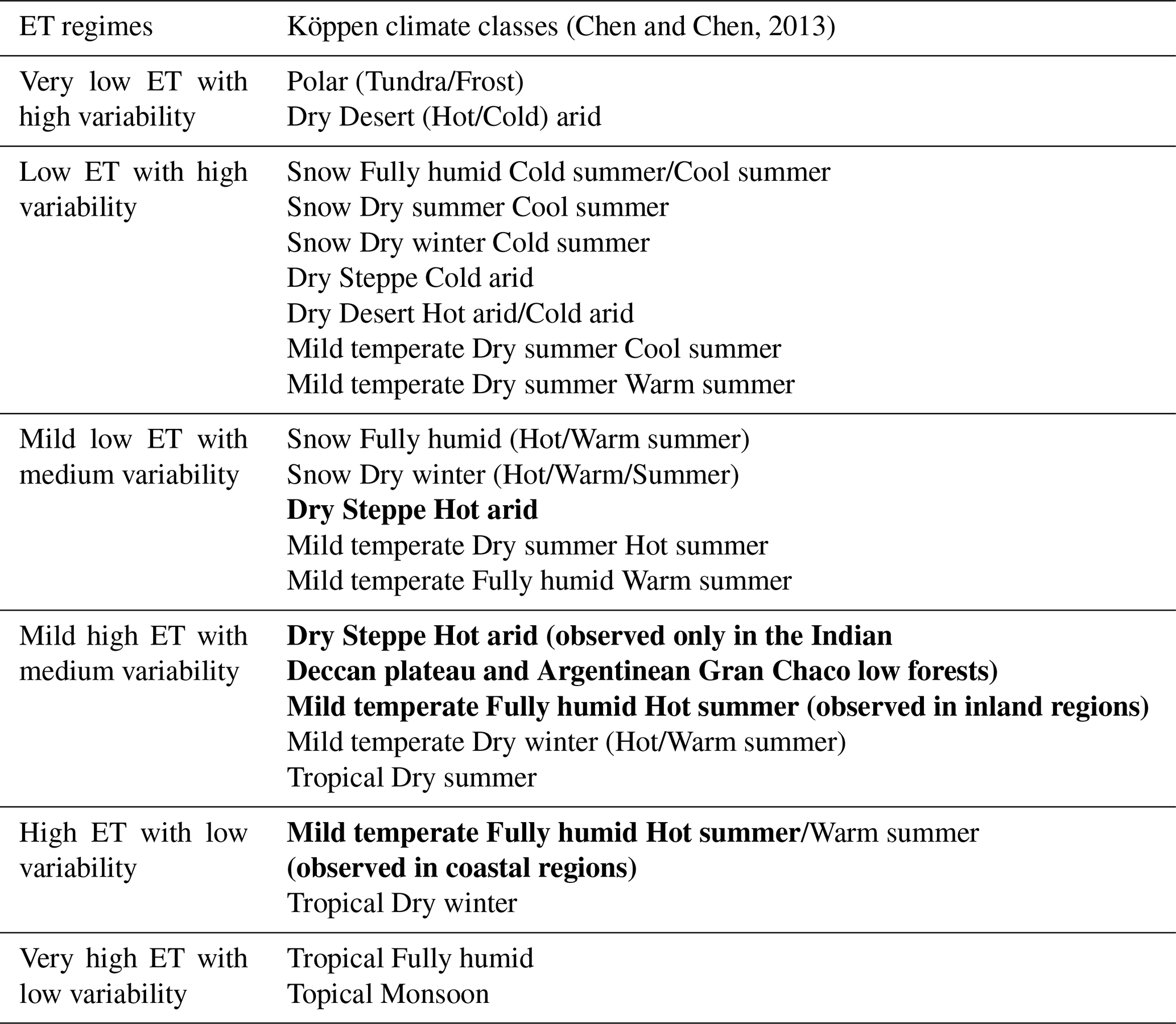
Table 4Correspondence between ET regimes derived here and Köppen climate classes derived in Chen and Chen (2013). Text in bold font indicates that the Köppen climate is associated with more than one ET regime.
3.5.2 ET regimes
To understand changes in ET across wet and dry regions, we classify land into six distinct dry and wet ET regimes according to two aspects of ET: annual averages and within-year relative variability derived from DOLCE V3. We apply K-means clustering (MacQueen, 1967) – an unsupervised machine learning algorithm known for its outstanding efficiency in clustering data – by implementing the K-Means function and the least squares quantisation method (Lloyd, 1982) using R software. K-Means identifies K centroids (i.e. imaginary values representing the centre of the clusters) and assigns each data point to the cluster of the nearest centroid using – in this paper – the least squares quantisation method. For each grid cell, we compute (1) the average of the annual total ET across 39 years (1980–2018) and (2) within-year relative variability climatology by temporally averaging the relative standard deviation of monthly ET calculated over a year and across all years. These have been used as input features for the unsupervised classification. After trial and error, we found that the global land can be adequately classified into six distinct regimes that include three dry and three wet regimes. According to centroids values (Table S4), we label the six regimes from driest to wettest, and we list the proportion of the land covered by each regime: (i) very low ET with high variability (16 %), (ii) low ET with high variability (34 %), (iii) mild low ET with medium variability (22 %), (iv) mild high ET with medium variability (13 %), (v) high ET with low variability (8 %) and (vi) very high ET with low variability (7 %). Figure 6 displays the spatial distribution of the six ET regimes.
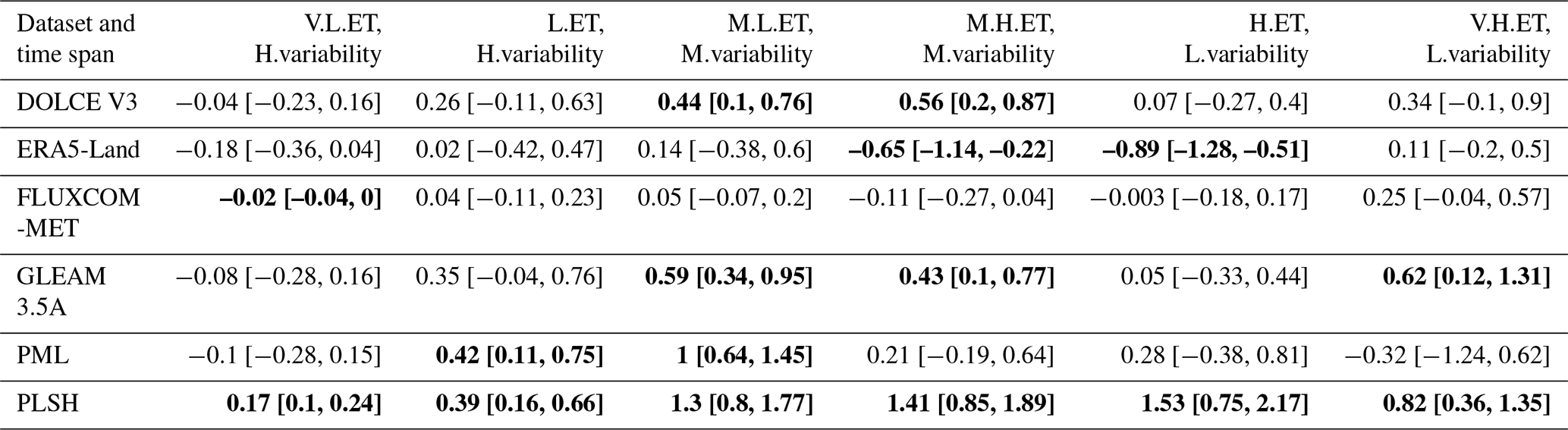
Table 5Trends in yearly ET total (mm yr−1) spatially averaged across each ET regime calculated for DOLCE V3 and five participating parent datasets available during 1982–2012. The text shows slopes of the trend line and their confidence intervals calculated at the 95 % confidence level; bold text indicates that the trend is reliable since the confidence interval is strictly positive or negative.
We compare the derived ET regimes map with the modified Köppen climate (KC) classification map by Chen and Chen (2013). We find that each KC class overlaps with only one ET regime with only two exceptions (Table 4): (i) land characterised by a “Dry Steppe Hot arid” (coded BSh in KC) climate belongs to the “Mild low ET with medium variability regime”, but in two regions, the Indian Deccan plateau and Argentinean Gran Chaco low forests, where the climate is BSh, the ET regime is “Mild high ET with medium variability”; (ii) Regions with a “Mild temperate Fully humid Hot summer” climate (coded Cfa in KC) overlap with the “Mild high ET with medium variability” regime in coastal regions and to the “Very high ET with low variability” regime in inland regions. These two KC classes (i.e. BSh and Cfa) are shown in bold in Table 4. Overall, ET regimes defined in this paper provide an efficient way to aggregate the KC classes into less varied classes. This is not surprising knowing that KC classes are developed based on the empirical relationship between climate and vegetation and that ET links the water, energy (climate) and carbon (vegetation) budgets.
3.5.3 Global annual trends across the ET regimes
We now explore annual trends in mean ET exhibited in each ET regime during 1980–2018. First, we calculate the annual ET total climatology and ET relative variability climatology spatially averaged across each regime separately; then we compute the trends in yearly ET as above (i.e. using Mann–Kendall and Sen's slope methods). Figure 7 illustrates trend results for the dry regimes (V.L.ET, H.variability, L.ET, H.variability and M.L.ET, M.Variability) and the wet regimes (M.H.ET, M.variability, H.ET, L.variability and V.H.ET, L.variability). Across all regimes except the wettest one, trends in yearly ET total are upward as indicated by the positive signs of both the slopes and their complete confidence intervals. The strongest trends occur in the “M.H.ET, M.variability” regime at a rate 0.6 mm yr−1, while the slowest trend occurs in the “V.L.ET H.variability” regime where ET is in general low. In the wettest ET regime “V.H. ET, L.variability”, while the slope of the trend is positive, its confidence interval contains mixed positive and negative values. This suggest that the tendency for increasing ET in the wettest ET regime is not robust. Our results indicate that decreasing ET trends observed in some regions oppose the consistent positive trends across the majority of ET clusters.
We repeat the same analysis for all the participating parent datasets that span at least 30 years. Sen's slope of the trends over the period 1982–2012 and their confidence interval (computed at the 95 % confidence level) are presented in Table 5. As noted earlier, trend behaviours are deemed inconclusive when the CI encompasses negative and positive values. These are presented with regular (as opposed to bold) typeface and are exhibited by FLUXCOM-MET in all regimes except the driest. In contrast, PLSH shows reliable upward trends in all regimes. ERA5-Land shows downward trends in the “M.H.ET, M.variability” and “H.ET, L.variability” regimes. Both GLEAM 3.5A and DOLCE V3 show reliable upward ET trends in the two middle regimes. Differences exist in the magnitude of trends across the majority of the products and the regimes. In DOLCE V3, the strongest trend occurs in the “M.H.ET, M.variability” regime at a rate of 0.56 mm yr−1. Finally, the slopes of DOLCE V3 trends are within the range of slopes of trends in available ET products.
There are of course some notable limitations to the approach we have taken here, some of which were previously discussed in Hobeichi et al. (2018). First, the weighting approach adopted here relies heavily on flux tower observations, which can suffer from a range of technical issues (Burba and Anderson, 2010; Fratini et al., 2019), as well as temporal gaps during particular weather conditions such as extremes (Van Der Horst et al., 2019), which can affect our results. Next, unresolved land surface processes in the parent datasets due, for example, to the absence of a proper representation of snow and permafrost dynamics or the heterogeneity of the land surface are likely to lead to uncertain ET estimation in DOLCE V2 and DOLCE V3, since each of these is only a combination of its parent datasets. This applies particularly in regions where observations are scarce or do not exist.
This work presents two new hybrid ET datasets DOLCE V2.1 and DOLCE V3. The new datasets are the result of several key improvements over their predecessor, incorporating more parent products in DOLCE V2.1, more in situ data, testing a range of alternative implementations of its weighting and bias-correction approach, increased spatial resolution, and covering a longer time period. The incorporation of a large ensemble of parent datasets in DOLCE V2.1 allowed us to derive a more optimal ET product that can be used to benchmark global ET estimates. In comparison, the reduced number of parent datasets in DOLCE V3 minimised temporal tiering and ensured that no temporal discontinuities occur throughout the covered period. This allowed us to examine historical trends in ET and their robustness to observational uncertainty. Despite the observationally constrained approach to defining uncertainty, we found robust ET trends across most areas of the land surface – enough to present a clear signal in most of the ET climate regimes we examined. These trends indicate a global increase in land-derived ET between 1980 and 2018. This contrasts with other gridded ET products that did not incorporate the same degree of observational constraint in either their mean field or uncertainty estimates, and demonstrates the usefulness of this long-term hybrid ET dataset.
The DOLCE V2.1 dataset (Hobeichi et al., 2020b) is publicly available in NetCDF-4 format and can be freely downloaded from the National Computational Infrastructure (NCI) data catalogue at https://doi.org/10.25914/5f1664837ef06.
The DOLCE V3 dataset (Hobeichi et al., 2021) is publicly available in NetCDF-4 format and can be freely downloaded from the NCI data catalogue at https://doi.org/10.25914/606e9120c5ebe.
The supplement related to this article is available online at: https://doi.org/10.5194/hess-25-3855-2021-supplement.
The ideas for this study originated in discussions with all authors. SH developed the new versions of the DOLCE dataset, performed the analyses, and mainly wrote the paper with input from GA. GA provided support with the collection of the in situ dataset. GA and JPE reviewed and edited the paper before submission.
The authors declare that they have no conflict of interest.
Publisher’s note: Copernicus Publications remains neutral with regard to jurisdictional claims in published maps and institutional affiliations.
The authors acknowledge the support of the Australian Research Council Centre of Excellence for Climate Extremes (CE170100023). This research was undertaken with the assistance of resources and services from the National Computational Infrastructure (NCI), which is supported by the Australian Government. We thank Franklin (Pete) Robertson (NASA Marshall Space Flight Center) for his valuable contribution to DOLCE V3. This work used eddy covariance data acquired and shared by the FLUXNET community, including these networks: AmeriFlux, AfriFlux, AsiaFlux, CarboAfrica, CarboEuropeIP, CarboItaly, CarboMont, ChinaFlux, Fluxnet-Canada, GreenGrass, ICOS, KoFlux, LBA, NECC, OzFlux-TERN, TCOS-Siberia and USCCC. The FLUXNET eddy covariance data processing and harmonisation were carried out by the ICOS Ecosystem Thematic Center, AmeriFlux Management Project and Fluxdata project of FLUXNET, with the support of Carbon Dioxide Information Analysis Center (CDIAC) and the OzFlux, ChinaFlux and AsiaFlux offices. Data were also obtained from the Atmospheric Radiation Measurement (ARM) Program sponsored by the U.S. Department of Energy, Office of Science, Office of Biological and Environmental Research, Climate and Environmental Sciences Division. This work used data sourced from the Terrestrial Ecosystem Research Network (TERN) infrastructure, which is an Australian Government National Collaborative Research Infrastructure Strategy (NCRIS)-enabled project; the Oak Ridge National Laboratory Distributed Active Archive Center (ORNL DAAC); and the Land Cover project of the ESA Climate Change Initiative. We would like to thank all the principal investigators that authorised us to download site data from the European Fluxes Database and all the research institutes that made publicly available and/or hosted the gridded ET datasets used in this study.
This research has been supported by the Australian Research Council Centre of Excellence for Climate Extremes (CE170100023).
This paper was edited by Ryan Teuling and reviewed by Jasper Denissen and one anonymous referee.
Abramowitz, G. and Bishop, C. H.: Climate model dependence and the ensemble dependence transformation of CMIP projections, J. Climate, 28, 2332–2348, https://doi.org/10.1175/JCLI-D-14-00364.1, 2015.
Abramowitz, G., Herger, N., Gutmann, E., Hammerling, D., Knutti, R., Leduc, M., Lorenz, R., Pincus, R., and Schmidt, G. A.: ESD Reviews: Model dependence in multi-model climate ensembles: weighting, sub-selection and out-of-sample testing, Earth Syst. Dynam., 10, 91–105, https://doi.org/10.5194/esd-10-91-2019, 2019.
Alemohammad, S. H., Fang, B., Konings, A. G., Aires, F., Green, J. K., Kolassa, J., Miralles, D., Prigent, C., and Gentine, P.: Water, Energy, and Carbon with Artificial Neural Networks (WECANN): a statistically based estimate of global surface turbulent fluxes and gross primary productivity using solar-induced fluorescence, Biogeosciences, 14, 4101–4124, https://doi.org/10.5194/bg-14-4101-2017, 2017.
Balsamo, G., Albergel, C., Beljaars, A., Boussetta, S., Brun, E., Cloke, H., Dee, D., Dutra, E., Muñoz-Sabater, J., Pappenberger, F., de Rosnay, P., Stockdale, T., and Vitart, F.: ERA-Interim/Land: a global land surface reanalysis data set, Hydrol. Earth Syst. Sci., 19, 389–407, https://doi.org/10.5194/hess-19-389-2015, 2015.
Bishop, C. H. and Abramowitz, G.: Climate model dependence and the replicate Earth paradigm, Clim. Dynam, 41, 885–900, https://doi.org/10.1007/s00382-012-1610-y, 2013.
Bodesheim, P., Jung, M., Gans, F., Mahecha, M. D., and Reichstein, M.: Upscaled diurnal cycles of land–atmosphere fluxes: a new global half-hourly data product, Earth Syst. Sci. Data, 10, 1327–1365, https://doi.org/10.5194/essd-10-1327-2018, 2018.
Burba, G. and Anderson, D. A.: brief practical guide to eddy covariance flux measurements: principles and workflow examples for scientific and industrial applications, Li-Cor Biosciences, Lincoln, Nebraska 68504, USA, 2010.
Candogan Yossef, N., van Beek, L. P. H., Kwadijk, J. C. J., and Bierkens, M. F. P.: Assessment of the potential forecasting skill of a global hydrological model in reproducing the occurrence of monthly flow extremes, Hydrol. Earth Syst. Sci., 16, 4233–4246, https://doi.org/10.5194/hess-16-4233-2012, 2012.
Chen, D. and Chen, H. W.: Using the Köppen classification to quantify climate variation and change: An example for 1901–2010, Environ. Dev., 6, 69–79, 2013.
Chen, X., Su, Z., Ma, Y., Yang, K., Wen, J., and Zhang, Y.: An improvement of roughness height parameterization of the Surface Energy Balance System (SEBS) over the Tibetan plateau, J. Appl. Meteorol. Climatol., 52, 607–622, https://doi.org/10.1175/JAMC-D-12-056.1, 2013.
Chen, X., Massman, W. J., and Su, Z.: A column canopy-air turbulent diffusion method for different canopy structures, J. Geophys. Res.-Atmos., 124, 488–506, 2019.
Dawdy, D. R., Lichty, R. W., and Bergmann, J. M.: A rainfall-runoff simulation model for estimation of flood peaks for small drainage basins, US Government Printing Office, Washington, USA, 1972.
Ershadi, A., McCabe, M. F., Evans, J. P., Chaney, N. W., and Wood, E. F.: Multi-site evaluation of terrestrial evaporation models using FLUXNET data, Agric. For. Meteorol., 187, 46–61, https://doi.org/10.1016/j.agrformet.2013.11.008, 2014.
Feng, F., Li, X., Yao, Y., Liang, S., Chen, J., Zhao, X., Jia, K., Pintér, K., and McCaughey, J. H.: An Empirical Orthogonal Function-Based Algorithm for Estimating Terrestrial Latent Heat Flux from Eddy Covariance, Meteorological and Satellite Observations, PLoS One, 11, e0160150, https://doi.org/10.1371/journal.pone.0160150, 2016.
Fisher, R. A. and Koven, C. D.: Perspectives on the future of Land Surface Models and the challenges of representing complex terrestrial systems, J. Adv. Model. Earth Syst., 12, 1–24, https://doi.org/10.1029/2018ms001453, 2020.
Fratini, G., Sabbatini, S., Ediger, K., Riensche, B., Burba, G., Nicolini, G., Vitale, D. and Papale, D.: Characterization of Eddy Covariance flux errors due to data synchronization issues during data acquisition, Geophys. Res. Abstr, 21, EGU General Assembly 2019, 2019.
Han, D., Wang, G., Liu, T., Xue, B.-L., Kuczera, G., and Xu, X.: Hydroclimatic response of evapotranspiration partitioning to prolonged droughts in semiarid grassland, J. Hydrol., 563, 766–777, 2018.
Herger, N., Abramowitz, G., Knutti, R., Angélil, O., Lehmann, K., and Sanderson, B. M.: Selecting a climate model subset to optimise key ensemble properties, Earth Syst. Dynam., 9, 135–151, https://doi.org/10.5194/esd-9-135-2018, 2018.
Hobeichi, S.: Conserving Land-Atmosphere Synthesis Suite (CLASS) v 1.1, https://doi.org/10.25914/5c872258dc183, 2019.
Hobeichi, S., Abramowitz, G., Evans, J., and Ukkola, A.: Derived Optimal Linear Combination Evapotranspiration (DOLCE): a global gridded synthesis ET estimate, Hydrol. Earth Syst. Sci., 22, 1317–1336, https://doi.org/10.5194/hess-22-1317-2018, 2018.
Hobeichi, S., Abramowitz, G., Evans, J., and Beck, H. E.: Linear Optimal Runoff Aggregate (LORA): a global gridded synthesis runoff product, Hydrol. Earth Syst. Sci., 23, 851–870, https://doi.org/10.5194/hess-23-851-2019, 2019.
Hobeichi, S., Abramowitz, G., and Evans, J. P.: Conserving Land – Atmosphere Synthesis Suite (CLASS ), J. Climate, 33, 1821–1844, https://doi.org/10.1175/JCLI-D-19-0036.1, 2020a.
Hobeichi, S., Abramowitz, G., and Evans, J. P.: Derived Optimal Linear Combination Evapotranspiration – DOLCE v2.1. NCI National Research Data Collection, https://doi.org/10.25914/5f1664837ef06, 2020b.
Hobeichi, S., Abramowitz, G., Contractor, S., and Evans, J.: Evaluating precipitation datasets using surface water and energy budget closure, J. Hydrometeorol., 21, 989–1009, https://doi.org/10.1175/jhm-d-19-0255.1, 2020c.
Hobeichi, S., Abramowitz, G., and Evans, J. P.: Derived Optimal Linear Combination Evapotranspiration – DOLCE v3.0. NCI National Research Data Collection, https://doi.org/10.25914/606e9120c5ebe, 2021.
Jiménez, C., Martens, B., Miralles, D. M., Fisher, J. B., Beck, H. E., and Fernández-Prieto, D.: Exploring the merging of the global land evaporation WACMOS-ET products based on local tower measurements, Hydrol. Earth Syst. Sci., 22, 4513–4533, https://doi.org/10.5194/hess-22-4513-2018, 2018.
Jung, M., Reichstein, M., Ciais, P., Seneviratne, S. I., Sheffield, J., Goulden, M. L., Bonan, G., Cescatti, A., Chen, J., De Jeu, R., Dolman, A. J., Eugster, W., Gerten, D., Gianelle, D., Gobron, N., Heinke, J., Kimball, J., Law, B. E., Montagnani, L., Mu, Q., Mueller, B., Oleson, K., Papale, D., Richardson, A. D., Roupsard, O., Running, S., Tomelleri, E., Viovy, N., Weber, U., Williams, C., Wood, E., Zaehle, S., and Zhang, K.: Recent decline in the global land evapotranspiration trend due to limited moisture supply, Nature, 467, 951–954, https://doi.org/10.1038/nature09396, 2010.
Jung, M., Koirala, S., Weber, U., Ichii, K., Gans, F., Gustau-Camps-Valls, Papale, D., Schwalm, C., Tramontana, G., and Reichstein, M.: The FLUXCOM ensemble of global land-atmosphere energy fluxes, Sci. Data, 6, 1–14, https://doi.org/10.1038/s41597-019-0076-8, 2019.
Kanamitsu, M., Ebisuzaki, W., Woollen, J., Yang, S.-K., Hnilo, J. J., Fiorino, M., and Potter, G. L.: NCEP-DOE AMIP-II Reanalysis (R-2), B. Am. Meteorol. Soc., 83, 1631–1644, https://doi.org/10.1175/BAMS-83-11-1631, 2002.
Kendall, M. G.: Rank correlation methods, Griffin, Oxford, England, 1948.
L'Ecuyer, T. S., Beaudoing, H. K., Rodell, M., Olson, W., Lin, B., Kato, S., Clayson, C. A., Wood, E., Sheffield, J., Adler, R., Huffman, G., Bosilovich, M., Gu, G., Robertson, F., Houser, P. R., Chambers, D., Famiglietti, J. S., Fetzer, E., Liu, W. T., Gao, X., Schlosser, C. A., Clark, E., Lettenmaier, D. P., and Hilburn, K.: The observed state of the energy budget in the early twenty-first century, J. Climate, 28, 8319–8346, https://doi.org/10.1175/JCLI-D-14-00556.1, 2015.
Liang, X., Lettenmaier, D. P., Wood, E. F., and Burges, S. J.: A simple hydrologically based model of land surface water and energy fluxes for general circulation models, J. Geophys. Res.-Atmos., 99, 14415–14428, https://doi.org/10.1029/94JD00483, 1994.
Lloyd, S.: Least squares quantization in PCM, IEEE Trans. Inf. theory, 28, 129–137, 1982.
Long, D., Longuevergne, L., and Scanlon, B. R.: Uncertainty in evapotranspiration fromland surfacemodeling, remote sensing, and GRACE satellites, Water Resour. Res., 50, 1131–1151, https://doi.org/10.1002/2013WR014581, 2014.
Lorenz, C., Tourian, M. J., Devaraju, B., Sneeuw, N., and Kunstmann, H.: Basin-scale runoff prediction: An Ensemble Kalman Filter framework based on global hydrometeorological data sets, Water Resour. Res., 51, 8450–8475, https://doi.org/10.1002/2014WR016794, 2015.
MacQueen, J.: Some methods for classification and analysis of multivariate observations, in: Proceedings of the fifth Berkeley symposium on mathematical statistics and probability, 1, 281–297, Oakland, CA, USA, 1967.
Mann, H. B.: Nonparametric tests against trend, Econom. J. Econom. Soc., 245–259, 1945.
Marengo, J. A., Souza, C. M., Thonicke, K., Burton, C., Halladay, K., Betts, R. A., Alves, L. M., and Soares, W. R.: Changes in Climate and Land Use Over the Amazon Region: Current and Future Variability and Trends, Front. Earth Sci., 6, 228, https://doi.org/10.3389/feart.2018.00228, 2018.
Martens, B., Miralles, D., Lievens, H., Van Der Schalie, R., De Jeu, R., Fernández-Prieto, D., and Verhoest, N.: GLEAM v3: updated land evaporation and root-zone soil moisture datasets, Geophys. Res. Abstr., EGU General Assembly 2016, 18, 2016–4253, 2016.
Martens, B., Miralles, D. G., Lievens, H., van der Schalie, R., de Jeu, R. A. M., Fernández-Prieto, D., Beck, H. E., Dorigo, W. A., and Verhoest, N. E. C.: GLEAM v3: satellite-based land evaporation and root-zone soil moisture, Geosci. Model Dev., 10, 1903–1925, https://doi.org/10.5194/gmd-10-1903-2017, 2017.
McCabe, M. F., Ershadi, A., Jimenez, C., Miralles, D. G., Michel, D., and Wood, E. F.: The GEWEX LandFlux project: evaluation of model evaporation using tower-based and globally gridded forcing data, Geosci. Model Dev., 9, 283–305, https://doi.org/10.5194/gmd-9-283-2016, 2016.
Michel, D., Jiménez, C., Miralles, D. G., Jung, M., Hirschi, M., Ershadi, A., Martens, B., McCabe, M. F., Fisher, J. B., Mu, Q., Seneviratne, S. I., Wood, E. F., and Fernández-Prieto, D.: The WACMOS-ET project – Part 1: Tower-scale evaluation of four remote-sensing-based evapotranspiration algorithms, Hydrol. Earth Syst. Sci., 20, 803–822, https://doi.org/10.5194/hess-20-803-2016, 2016.
Miralles, D. G., Holmes, T. R. H., De Jeu, R. A. M., Gash, J. H., Meesters, A. G. C. A., and Dolman, A. J.: Global land-surface evaporation estimated from satellite-based observations, Hydrol. Earth Syst. Sci., 15, 453–469, https://doi.org/10.5194/hess-15-453-2011, 2011a.
Miralles, D. G., De Jeu, R. A. M., Gash, J. H., Holmes, T. R. H., and Dolman, A. J.: Magnitude and variability of land evaporation and its components at the global scale, Hydrol. Earth Syst. Sci., 15, 967–981, https://doi.org/10.5194/hess-15-967-2011, 2011b.
Miralles, D. G., Van Den Berg, M. J., Gash, J. H., Parinussa, R. M., De Jeu, R. A. M., Beck, H. E., Holmes, T. R. H., Jiménez, C., Verhoest, N. E. C., Dorigo, W. A., Teuling, A. J., and Johannes Dolman, A.: El Niño-La Niña cycle and recent trends in continental evaporation, Nat. Clim. Change, 4, 122–126, https://doi.org/10.1038/nclimate2068, 2014.
Mu, Q., Zhao, M., and Running, S. W.: Improvements to a MODIS global terrestrial evapotranspiration algorithm, Remote Sens. Environ., 115, 1781–1800, https://doi.org/10.1016/j.rse.2011.02.019, 2011.
Mueller, B., Seneviratne, S. I., Jimenez, C., Corti, T., Hirschi, M., Balsamo, G., Ciais, P., Dirmeyer, P., Fisher, J. B., Guo, Z., Jung, M., Maignan, F., McCabe, M. F., Reichle, R., Reichstein, M., Rodell, M., Sheffield, J., Teuling, A. J., Wang, K., Wood, E. F., and Zhang, Y.: Evaluation of global observations-based evapotranspiration datasets and IPCC AR4 simulations, Geophys. Res. Lett., 38, 3–10, https://doi.org/10.1029/2010GL046230, 2011.
Mueller, B., Hirschi, M., Jimenez, C., Ciais, P., Dirmeyer, P. A., Dolman, A. J., Fisher, J. B., Jung, M., Ludwig, F., Maignan, F., Miralles, D. G., McCabe, M. F., Reichstein, M., Sheffield, J., Wang, K., Wood, E. F., Zhang, Y., and Seneviratne, S. I.: Benchmark products for land evapotranspiration: LandFlux-EVAL multi-data set synthesis, Hydrol. Earth Syst. Sci., 17, 3707–3720, https://doi.org/10.5194/hess-17-3707-2013, 2013.
Munier, S., Aires, F., Schlaffer, S., Prigent, C., Papa, F., Maisongrande, P., and Pan, M.: Combining datasets of satellite retrieved products for basin-scale water balance study. Part II: Evaluation on the Mississippi Basin and closure correction model, J. Geophys. Res.-Atmos., 119, 12100–12116, https://doi.org/10.1002/2014JD021953, 2014.
Muñoz Sabater, J.: ERA5-Land monthly averaged data from 1981 to end of 2018, Copernicus Climate Change Service (C3S) Climate Data Store (CDS), https://doi.org/10.24381/cds.68d2bb30, 2019.
Paca, V. H. d. M., Espinoza-Dávalos, G. E., Hessels, T. M., Moreira, D. M., Comair, G. F., and Bastiaanssen, W. G. M.: The spatial variability of actual evapotranspiration across the Amazon River Basin based on remote sensing products validated with flux towers, Ecol. Process., 8, 1–20, https://doi.org/10.1186/s13717-019-0158-8, 2019.
Pan, M., Sahoo, A. K., Troy, T. J., Vinukollu, R. K., Sheffield, J., and Wood, E. F.: Multisource estimation of long-term terrestrial water budget for major global river basins, J. Climate, 25, 3191–3206, https://doi.org/10.1175/JCLI-D-11-00300.1, 2012.
Pan, S., Pan, N., Tian, H., Friedlingstein, P., Sitch, S., Shi, H., Arora, V. K., Haverd, V., Jain, A. K., Kato, E., Lienert, S., Lombardozzi, D., Nabel, J. E. M. S., Ottlé, C., Poulter, B., Zaehle, S., and Running, S. W.: Evaluation of global terrestrial evapotranspiration using state-of-the-art approaches in remote sensing, machine learning and land surface modeling, Hydrol. Earth Syst. Sci., 24, 1485–1509, https://doi.org/10.5194/hess-24-1485-2020, 2020.
Quesada-Montano, B., Wetterhall, F., Westerberg, I. K., Hidalgo, H. G., and Halldin, S.: Characterising droughts in Central America with uncertain hydro-meteorological data, Theor. Appl. Climatol., 137, 2125–2138, https://doi.org/10.1007/s00704-018-2730-z, 2019.
Rodell, M., Beaudoing, H. K., L'Ecuyer, T. S., Olson, W. S., Famiglietti, J. S., Houser, P. R., Adler, R., Bosilovich, M. G., Clayson, C. A., Chambers, D., Clark, E., Fetzer, E. J., Gao, X., Gu, G., Hilburn, K., Huffman, G. J., Lettenmaier, D. P., Liu, W. T., Robertson, F. R., Schlosser, C. A., Sheffield, J., and Wood, E. F.: The observed state of the water cycle in the early twenty-first century, J. Climate, 28, 8289–8318, https://doi.org/10.1175/JCLI-D-14-00555.1, 2015.
Sahoo, A. K., Pan, M., Troy, T. J., Vinukollu, R. K., Sheffield, J., and Wood, E. F.: Reconciling the global terrestrial water budget using satellite remote sensing, Remote Sens. Environ., 115, 1850–1865, https://doi.org/10.1016/j.rse.2011.03.009, 2011.
Sen, P. K.: Estimates of the regression coefficient based on Kendall's tau, J. Am. Stat. Assoc., 63, 1379–1389, 1968.
Sharma, A., Wasko, C., and Lettenmaier, D. P.: If precipitation extremes are increasing, why aren't floods?, Water Resour. Res., 54, 8545–8551, 2018.
Sheffield, J., Wood, E. F., and Roderick, M. L.: Little change in global drought over the past 60 years, Nature, 491, 435–438, https://doi.org/10.1038/nature11575, 2012.
Stackhouse Jr., P. W., Gupta, S. K., Cox, S. J., Zhang, T., Mikovitz, J. C., and Hinkelman, L. M.: 24.5-Year surface radiation budget data set released, Glob. Energy Water Cycle Exp. News, 21, 1–20, 2011.
Stephens, G. L., Li, J., Wild, M., Clayson, C. A., Loeb, N., Kato, S., L'Ecuyer, T., Stackhouse, P. W., Lebsock, M., and Andrews, T.: An update on Earth's energy balance in light of the latest global observations, Nat. Geosci., 5, 691–696, https://doi.org/10.1038/ngeo1580, 2012.
Su, Z.: The Surface Energy Balance System (SEBS) for estimation of turbulent heat fluxes, Hydrol. Earth Syst. Sci., 6, 85–100, https://doi.org/10.5194/hess-6-85-2002, 2002.
Teuling, A. J.: A hot future for European droughts, Nat. Clim. Chang., 8, 364–365, 2018.
Teuling, A. J., Van Loon, A. F., Seneviratne, S. I., Lehner, I., Aubinet, M., Heinesch, B., Bernhofer, C., Grünwald, T., Prasse, H., and Spank, U.: Evapotranspiration amplifies European summer drought, Geophys. Res. Lett., 40, 2071–2075, 2013.
Ukkola, A. M., Pitman, A. J., Donat, M. G., De Kauwe, M. G., and Angélil, O.: Evaluating the Contribution of Land-Atmosphere Coupling to Heat Extremes in CMIP5 Models, Geophys. Res. Lett., 45, 9003–9012, https://doi.org/10.1029/2018GL079102, 2018.
van der Horst, S. V. J., Pitman, A. J., De Kauwe, M. G., Ukkola, A., Abramowitz, G., and Isaac, P.: How representative are FLUXNET measurements of surface fluxes during temperature extremes?, Biogeosciences, 16, 1829–1844, https://doi.org/10.5194/bg-16-1829-2019, 2019.
Vinukollu, R. K., Wood, E. F., Ferguson, C. R., and Fisher, J. B.: Global estimates of evapotranspiration for climate studies using multi-sensor remote sensing data: Evaluation of three process-based approaches, Remote Sens. Environ., 115, 801–823, https://doi.org/10.1016/j.rse.2010.11.006, 2011.
Wan, Z., Zhang, K., Xue, X., Hong, Z., Hong, Y., and Gourley, J.: Water balance-based actual evapotranspiration reconstruction fromground and satellite observations over the conterminous United States Zhanming, Water Resour. Res., 51, 6485–6499, https://doi.org/10.1002/2015WR017311, 2015.
Zhang, K., Kimball, J. S., Nemani, R. R., and Running, S. W.: A continuous satellite-derived global record of land surface evapotranspiration from 1983 to 2006, Water Resour. Res., 46, W09522, https://doi.org/10.1029/2009WR008800, 2010.
Zhang, K., Kimball, J. S., Nemani, R. R., Running, S. W., Hong, Y., Gourley, J. J., and Yu, Z.: Vegetation Greening and Climate Change Promote Multidecadal Rises of Global Land Evapotranspiration, Sci. Rep., 5, 1–9, https://doi.org/10.1038/srep15956, 2015.
Zhang, Y., Peña-Arancibia, J. L., McVicar, T. R., Chiew, F. H. S., Vaze, J., Liu, C., Lu, X., Zheng, H., Wang, Y., Liu, Y. Y., Miralles, D. G., and Pan, M.: Multi-decadal trends in global terrestrial evapotranspiration and its components, Sci. Rep., 6, 19124, https://doi.org/10.1038/srep19124, 2016.
Zhang, Y., Pan, M., Sheffield, J., Siemann, A. L., Fisher, C. K., Liang, M., Beck, H. E., Wanders, N., MacCracken, R. F., Houser, P. R., Zhou, T., Lettenmaier, D. P., Pinker, R. T., Bytheway, J., Kummerow, C. D., and Wood, E. F.: A Climate Data Record (CDR) for the global terrestrial water budget: 1984–2010, Hydrol. Earth Syst. Sci., 22, 241–263, https://doi.org/10.5194/hess-22-241-2018, 2018.