the Creative Commons Attribution 4.0 License.
the Creative Commons Attribution 4.0 License.
 | 02 Jul 2021
Conditional simulation of spatial rainfall fields using random mixing: a study that implements full control over the stochastic process
Jieru Yan
Fei Li
András Bárdossy
Tao Tao
The accuracy of spatial precipitation estimates with relatively high spatiotemporal resolution is of vital importance in various fields of research and practice. Yet the intricate variability and intermittent nature of precipitation make it very difficult to obtain accurate spatial precipitation estimates. Radars and rain gauges are two complementary sources of precipitation information: the former are inaccurate in general but are valid indicators of the spatial pattern of the rainfall field; the latter are relatively accurate but lack spatial coverage. Several radar–gauge merging techniques that can provide spatial precipitation estimates have been proposed in the scientific literature. Conditional simulation has great potential to be used in spatial precipitation estimation. Unlike commonly used interpolation methods, conditional simulation yields a range of possible estimates due to its Monte Carlo framework. However, one obstacle that hampers the application of conditional simulation in spatial precipitation estimation is the need to obtain the marginal distribution function of the rainfall field with sufficient accuracy. In this work, we propose a method to obtain the marginal distribution function from radar and rain gauge data. A conditional simulation method, random mixing (RM), is used to simulate rainfall fields. The radar and rain gauge data used in the application of the proposed method are derived from a stack of synthetic rainfall fields. Due to the full control over the stochastic process, the accuracy of the estimates is verified comprehensively. The results from the proposed approach are compared with those from three well-known radar–gauge merging techniques: ordinary Kriging, Kriging with external drift, and conditional merging, and the sensitivity of the approach to two factors – the number of rain gauges and the random error in the radar estimates – is analysed in the same experimental context.
- Article
(3152 KB) - Full-text XML
- BibTeX
- EndNote


Precipitation is one of the most important factors in hydrology and meteorology. The accuracy of spatial precipitation estimates with relatively high spatiotemporal resolution is of vital importance in various fields of research and practice, such as the promotion of meteorological and hydrological monitoring, forecasting performed to enhance our ability to cope with natural disasters, the study of climate trends and variability, and the management of water resources (Yilmaz et al., 2005; Michaelides et al., 2009; Jiang et al., 2012; Liu et al., 2017). Yet, unlike many other hydrometeorological variables such as temperature and humidity, precipitation occurs intermittently in space and time, i.e. nonrainy areas occur amidst rainy areas, and dry periods occur amidst wet periods (Kumar and Foufoula-Georgiou, 1994). The intricate spatiotemporal variability and intermittent nature of precipitation make it very difficult to obtain accurate spatial precipitation estimates (Emmanuel et al., 2012; Cristiano et al., 2017).
Rain gauges – the only devices that directly measure precipitation on the ground surface – are still considered the most reliable source of precipitation information in hydrology. However, rain gauges are only available at limited locations. The representativeness of gauge observations for the entire precipitation field is therefore limited. Significant research has shown that precipitation estimation based on gauge observations suffers from degraded levels of accuracy during storms with increased rainfall intensities, when convective processes are significant (Adams, 2016). Meteorological radar, on the other hand, is a superb tool for measuring spatial patterns of reflectivity at the altitude of the measurement. Yet radar-based precipitation estimation can be problematic due to various sources of errors, e.g. variations in the vertical profile reflectivity (VPR), static/dynamic clutter, signal attenuation, anomalous propagation of the beam, and uncertainty about the Z–R relationship (see Doviak and Zrnić, 1993; Collier, 1999; Fabry, 2015, for details). Despite these various potential error sources, radar-based precipitation estimation is still, however, considered a valid indicator of precipitation patterns (Méndez Antonio et al., 2009; Yan et al., 2020). In summary, radars and rain gauges are two complementary sources of precipitation information: the former are inaccurate in general but are valid indicators of the spatial pattern of the rainfall field; the latter are relatively accurate but lack spatial coverage.
Considering the pros and cons of the two sources of precipitation information, many radar–gauge merging techniques to obtain spatial precipitation estimates have been developed in recent years. Wang et al. (2013) grouped these techniques into two categories: bias reduction techniques and error variance minimization techniques. Bias reduction techniques attempt to correct the bias of radar rainfall estimates using rain gauge observations. This class of techniques has a long history; they range from the earliest mean field bias correction schemes where a single correction factor is applied to the entire radar field (e.g. Wilson, 1970) to later local bias correction schemes where spatially distributed correction factors are applied (e.g. Brandes, 1975; James et al., 1993; Michelson and Koistinen, 2000). Error variance minimization techniques attempt to eliminate the bias of radar rainfall estimates while minimizing the variance between radar and rain gauge measurements. Representatives of this class include the Bayesian data combination scheme (Todini, 2001), Kriging-based techniques such as conditional merging (Sinclair and Pegram, 2005), Kriging with external drift (Hengl et al., 2003; Haberlandt, 2007; Velasco-Forero et al., 2009), and co-Kriging (Schuurmans et al., 2007; Sideris et al., 2014).
In addition to the two categories mentioned above, there is a class of methods that simulate spatial random fields under the Monte Carlo framework. The logic behind the use of such methods is straightforward. When faced with uncertainty during the process of making a forecast or estimation, rather than replacing the uncertain variable with a single average number, simulation can provide a better solution by yielding a range of possible outcomes. In the context of merging radar and rain gauge data, simulation is often performed under constraints (such as equality constraints at rain gauge locations or the field pattern indicated by radar). There are several methods that simulate spatially random fields using certain covariance functions in Gaussian space, such as turning bands simulation, LU-decomposition-based methods, and sequential Gaussian simulation (Mantoglou and Wilson, 1982; Deutsch and Journel, 1998; Chilès and Delfiner, 2000; Lantuéjoul, 2002). Studies on conditional simulation of rainfall fields are, however, rare. One of the major obstacles that hampers the application of conditional simulation in spatial precipitation estimation is the need to obtain the marginal distribution function of the rainfall field with sufficient accuracy. This distribution function is needed to transform the simulated Gaussian fields to rainfall fields of interest, as the simulation is normally embedded in Gaussian space. Given this, in the present paper, we propose a method to obtain the distribution function from radar and rain gauge data.
Here, the method we employ to simulate rainfall fields is random mixing (RM), which was first proposed by Bárdossy and Hörning (2016) to solve inverse modelling problems encountered when modelling groundwater flow and transport. RM uses the concept employed in the gradual deformation (GD) approach described in Hu (2000): that a conditional field of interest can be obtained as a linear combination of unconditional random fields. However, unlike GD, RM is targeted and flexible enough to be able to incorporate different kinds of constraints (linear or nonlinear), and the utilization of spatial copulas in the description of the underlying dependence structure enables the dependence structure and marginal distribution to be treated separately.
The radar and rain gauge data used when applying the proposed approach in this study are derived from a stack of synthetic rainfall fields. Compared to commonly used verification methods (e.g. leave-n-out cross-validation, where the accuracy of the estimates is verified at limited locations), the accuracy of the estimates is verified more comprehensively in this study, as the synthetic data used allows full control over the stochastic process. The results from the proposed approach are compared with those from several well-known radar–gauge merging techniques: ordinary Kriging, Kriging with external drift, and conditional merging. Finally, the sensitivity of the proposed approach to two factors – the number of rain gauges and the random error in the radar estimates – is analysed.
This paper is divided into six parts. After this introductory section, the methodology of RM is elaborated in Sect. 2. Section 3 describes the data used in this study. Section 4 compares the results from the proposed approach with those obtained from other techniques and analyses the sensitivity of the approach. Section 5 describes the scope and assumptions of the approach and discusses the limitations of this study. Section 6 draws conclusions and presents the outlook for the proposed approach.
2.1 CDF of the rainfall field
As described in the “Introduction”, one of the major obstacles to the application of conditional simulation in spatial precipitation estimation is obtaining the cumulative distribution function of the rainfall field (rainfall CDF hereafter) with sufficient accuracy. The rainfall CDF is needed to transform the simulated Gaussian fields to rainfall fields of interest. In this subsection, an algorithm to compute the rainfall CDF from radar and rain gauge data is proposed. The algorithm is as follows:
-
Estimate the spatial intermittency of the rainfall field as the ratio of the number of dry pixels to the total number of pixels in the radar estimates Rr. We denote the estimated spatial intermittency by u0.
-
Transform the radar estimates Rr to nonexceedance probabilities (termed quantiles hereafter), which results in a quantile map. Due to the intermittent nature of precipitation, all the dry pixels in Rr are transformed to u0 (i.e. u0 is the smallest value in the quantile map).
-
Determine the gauge-respective quantiles in the radar quantile map, which are denoted by uk for k=1, …, K. The two datasets – the rain gauge observations rk and the gauge-respective quantiles uk – form K pairs (rk, uk). Perform the following quality control steps for these pairs:
-
Check the consistency at zeros and remove the pair whenever a zero is encountered, i.e. rk=0 or uk=u0. In the ideal case where the radar estimates perfectly represent the pattern of the rainfall field, zero gauge observations and the smallest quantile u0 should coexist. However, in practice, there are various factors that can reduce the representativeness of the radar-indicated field pattern. A zero gauge observation could be collocated with a quantile that is slightly larger than u0, and a dry pixel could be collocated with a gauge observation that is slightly larger than 0 mm. The consistency at zeros is an important indicator of the mismatch between the radar and rain gauge data, though none of the zeros in the two datasets are used in the computation of the rainfall CDF.
-
Maintain consistency in order. In the ideal case described in the previous item, the pairs (rk, uk) represent K points that are exactly on the rainfall CDF. However, due to the degraded representativeness of the radar estimates, the Spearman rank correlation of rk and uk can be less than 1. Namely, the two datasets have different orders; for example, the largest rain gauge observation does not correspond to the largest radar quantile. To maintain a consistent order, the values in rk and uk that remain after applying the first item are sorted in ascending order.
Note that both of these consistencies (consistency at zeros and consistency in order) are good indicators of the mismatch between radar and rain gauge data. A significant mismatch – e.g. the collocation of a dry pixel with a 5 mm rainfall record, or a low Spearman's rank correlation (say ρr<0.8) – can lead to unreliable estimates.
-
-
After performing the quality control steps, it is assumed that the set of points (rk, uk) are distributed without bias around the true CDF; see the empirical CDF obtained by linearly joining the points in Fig. 1. The rainfall CDF is obtained by fitting a theoretical CDF model under the condition that the fitted CDF becomes positive at the point (0, u0). The estimated rainfall CDF is denoted by G(⋅) hereafter.
In the above algorithm, the radar data provide a hint about the representativeness of the rain gauge data. For example, has the extreme of the rainfall field been properly sampled by the gauges? If not, to what extent has the extreme been underestimated by the samples (rain gauge observations)? One could answer this question by checking the maximum value among the gauge-respective radar quantiles. Similarly, one could also find the answers to questions such as whether the samples are uniformly distributed in terms of the quantile range or whether they just gather around the lower/higher range of the rainfall field. Without the additional information provided by radar, one would probably assign evenly distributed quantiles to the rain gauge observations, as usually done in the acquisition of the empirical CDF.

Figure 1Light grey: the empirical CDFs obtained by linearly joining (rk, uk) points after the two quality control steps, with one CDF highlighted by the black dashed line. Red: the true rainfall CDF. Note that the empirical CDFs shown here are computed from the synthetic data as described in Sect. 3.
2.2 Prepare the constraints
The simulation is embedded in Gaussian space; hence, the constraints should be transformed to the standard normal marginal (normalized Gaussian). Specifically, we consider the following three constraints:
-
The equality constraints at rain gauge locations, when defined in terms of the standard normal marginal, mean that the simulated values at the rain gauge locations should equal the values mapped from the rain gauge observations rk:
where Z is the simulated Gaussian field, xk denotes the rain gauge location, and G(⋅) and Φ(⋅) denote the rainfall CDF and the CDF of the standard normal distribution, respectively.
-
The simulated Gaussian field Z should preserve a given correlation function obtained from the transformed radar estimates, i.e.
The problem here is that one can only obtain a truncated Gaussian field from the radar estimates Rr, as all the dry pixels in Rr are converted to , where u0 is the spatial intermittency. The sill of the correlation function evaluated from is reduced due to the truncation. Figure 2 displays and compares empirical variograms evaluated from 1000 truncated Gaussian fields with the true variogram used to generate the corresponding continuous Gaussian fields. From the figure, it can be seen that the empirical and true variograms have very similar patterns. Practically speaking, the true correlation function can be approximated by scaling given a priori knowledge that the variance of the simulated field is 1. Besides, as random mixing is a geostatistical simulation method, the choice of the correlation function has a limited effect on the estimates, just as it does for Kriging (Verworn and Haberlandt, 2011). We denote the estimated correlation function by Γ hereafter.
Note that the terms correlation function and variogram are used interchangeably here, as it is common in geostatistics to work with the variogram, the estimation of which has been shown to be more stable than that of the correlation function (Calder and Cressie, 2009). Namely, one simulates by using the correlation function as the measure of spatial dependence, whereas the spatial dependence of the simulated field is normally examined via its variogram.
-
The pattern of the simulated field should resemble that of the radar estimates as closely as possible. This represents an optimization problem, and the goal is to maximize the Pearson correlation coefficient of the simulated field Z and the reference field , i.e.
where Z is the simulated Gaussian field, is obtained from the radar estimates as defined in Eq. (2), and ρ(⋅) is the Pearson correlation coefficient. The same problem arises: Z is continuous whereas is truncated. To evaluate the objective function, one could truncate Z at z0 or one could also use Z directly, as shown in Eq. (3). The difference between these approaches is minor, as a high correlation between and Z means a high correlation between and the truncated Z. To be as parsimonious as possible, we use Z directly in the evaluation of the objective function.

Figure 2The blue lines denote the empirical variograms evaluated from 1000 truncated Gaussian fields; the 95 % confidence interval is marked by the black dashed lines. The red line denotes the true variogram used to generate the continuous Gaussian fields. Note that the continuous Gaussian field is truncated at .
2.3 Random mixing
The task is to estimate the true rainfall field given a set of rain gauge observations and a set of radar estimates. In terms of conditional simulation, this means simulating a Gaussian field Z that fulfils all the constraints described in Sect. 2.2 and then converting Z to the rainfall field of interest, i.e. yielding an estimate of the true rainfall field.
We use random mixing (RM) to fulfil the task. RM utilizes the concept described in Hu (2000): that the conditional field of interest can be obtained as a linear combination of many unconditional random fields, i.e.
where Yi(s) are independent Gaussian random fields with identical statistical properties, i.e. the marginal distributions all follow the standard normal distribution with the same correlation function. If, in addition, the L2 norm of the weights αi fulfils
the resultant conditional field Z is statistically identical to Yi, as demonstrated by Bárdossy and Hörning (2016). There are several methods that can be used to obtain Gaussian random fields with a given correlation function. We have used an efficient method – the fast Fourier transform for regular grids (Wood and Chan, 1994; Wood, 1995; Ravalec et al., 2000).
It is necessary to differentiate Hu's method from the proposed one before specifying the algorithm. Hu's method (Hu, 2000; Hu et al., 2001) incorporates linear data using conditional Kriging, and the method is extended to combine dependent conditional fields in Hu (2002), whereas RM incorporates linear or nonlinear constraints under the unified concept of randomly mixing unconditional random fields. The algorithm for RM is as follows:
-
The prospective conditional Gaussian field Z that fulfils all the constraints is obtained as
Z consists of two parts:
- a.
The first part,
is made up of N statistically identical unconditional random fields Yi(s) with correlation function Γ, as estimated in Sect. 2.2. The role of this part is to fulfil the equality constraints at the rain gauge locations. Thus, K linear constraints are imposed as
See Eq. (1) for the definitions of xk, rk, G(⋅) and . In total, we have N unknowns: αi for i=1, …, N and K equations. If N>K, this forms an underdetermined equation system. Multiple techniques are available for solving such a system. Specifically, we found the set of weights with the lowest L2 norm; i.e. we minimized by using the singular value decomposition technique. In addition, the constraint is imposed to ensure that the second part has a positive weight, i.e. . The extra constraint is further satisfied by increasing N, i.e. increasing the number of degrees of freedom of the equation system.
- b.
The second part,
is made up of two independent, statistically identical conditional random fields H and H′, which are referred to as the H-field hereafter. The H-field is also obtained as a linear combination of unconditional random fields (statistically identical to Yi):
The H-field is special because of the zeros at the rain gauge locations, which mean that the addition of the second part to the first part does not change the values at the rain gauge locations. Hence, the equalities in Eq. (7) can be rewritten as
The remaining question is how to obtain such H-fields. Similarly, an underdetermined system is created as
with M unknowns, K equations, and M>K. To ensure that the H-field is statistically identical to Y′ (or Y), the following constraint is imposed additionally:
The set of weights (βi for i=1, …, M) can be determined by solving Eq. (9) first, and then scaling the weights with the factor () such that Eq. (10) is satisfied. Because of the “zeros”, scaling does not change the values at the rain gauge locations.
The Gaussian field Z obtained from Eq. (6) fulfils the equality constraints at the rain gauge locations and reproduces the correlation function Γ. The correlation function is reproduced because the L2 norm of the weights of all the fields underlying Z satisfies
It should be noted that one H-field is sufficient to do the same job. For example, one could obtain such a Z via
The aim of using two H-fields instead of one is to introduce more freedom, allowing the third constraint to be met too. The relative weights of the two parts () do matter. The second part should weigh more, as this facilitates the solution of the optimization problem defined in the next step. Thus, when solving the underdetermined system in (a), the set of weights is found.
- a.
-
Due to the freedom introduced by the extra H-field, the Gaussian field Z obtained from Eq. (6) is a function of θ. This is also true of the objective function evaluated from Z, which actually defines a 1D optimization problem w.r.t. θ:
where . See the definitions of and ρ(⋅) in Eqs. (2) and (3). The task is to find the θ that produces the maximum objective function value. There are various methods that can be applied to solve the 1D unconstrained optimization problem. In this work, we simply used the trial-and-error method, and a coarse search followed by a fine search was implemented to accelerate the solving process. The solution to the 1D optimization problem is denoted by θ*.
-
If Z(θ*) meets the stopping criterion of the optimization, continue with step 4. Otherwise, go back to step 2 after updating H and H′ as follows:
As always in optimization, there are multiple choices of stopping criteria, such as a particular number of iterations, a preset limit on the objective function, a specific rate of decrease of the objective function, and so forth. We adopted a specific number of continuous iterations without improvement as the stopping criterion.
-
Finally, an estimate of the true rainfall field is obtained as
An artificial experiment was carried out to test the capability of the proposed approach to estimate the true rainfall field. Due to a lack of knowledge of the true fields, we used synthetic ones: 1000 rainfall fields were generated independently and served as the “true” rainfall fields from which the radar and rain gauge data were derived.
This was done because it is difficult to verify the accuracy of the estimates comprehensively without knowing the real rainfall field. Some studies employ the leave-n-out cross-validation method, where one verifies the accuracy of the estimates at certain points, for verification. However, the accuracy of the estimates in terms of the overall statistics (e.g. the mean and maximum of the rainfall field) is more hydrologically interesting than the accuracy at particular points.
3.1 Generate the true rainfall fields
1000 rainfall fields, each with a grid size of 80×80, were generated. Each pixel was assumed to represent an area of 1×1 km2, and all 1000 fields were generated independently and had identical properties, i.e. they all had the same spatial intermittency, rainfall CDF, and correlation function. The generation procedure was as follows:
-
Generate 1000 Gaussian random fields ZT with a given correlation function. Figure 3a displays the exponential correlation function used in the generation of ZT. Note that a subscript T is used throughout this paper to denote the true Gaussian and rainfall fields or the true rainfall CDF. Similarly, we used the fast Fourier transform for regular grids to generate ZT.
-
Generate a rainfall CDF where the lognormal distribution is used as the model for the rainfall CDF, as this distribution has been shown to be effective at describing the marginal distribution of rainfall rates or the short-time rainfall (accumulation time: 10 or 15 min) over a specified area (Bell, 1987; Crane, 1990; Pegram and Clothier, 2001). Figure 3b shows the rainfall CDF used in the generation of the 1000 true rainfall fields, i.e. the true rainfall CDF: .
-
Convert the Gaussian random fields ZT to rainfall fields using the normal-score transformation method:
where RT is the true rainfall field and Φ(⋅) is the CDF of the standard normal distribution. Note that the quantile value u0, which is labelled in Fig. 3b, is used to maintain the spatial intermittency. Hence, all pixel values smaller than in ZT are converted to zero (precipitation) in RT.

Figure 3(a) The exponential correlation function used in the generation of the Gaussian random fields ZT. (b) The rainfall CDF used in the generation of the true rainfall fields, where the spatial intermittency u0 is labelled.
3.2 Generate the radar estimates
The radar estimates were derived from the true rainfall fields. Specifically, the Gaussian field ZT generated in Sect. 3.1 was used. Two types of errors are commonly seen in radar estimates: random and nonlinear errors. The following procedure was applied to mimic those errors:
-
Introduce a random error. The proposed approach assumes that the radar estimates measured aloft can represent the pattern of the rainfall field on the ground. However, there are some factors that can reduce the representativeness of radar estimates, such as evaporation, complex terrain effects, and anthropogenic effects. A random error is therefore introduced to mimic this kind of error. We also utilize the concept of random mixing, where the Gaussian field with the introduced random error is obtained by mixing two fields:
where ZT is the true Gaussian field and Ze is an independently generated Gaussian random field with the same statistical properties as ZT. The constraint is also imposed to ensure that the resultant Zr is statistically identical to ZT (or Ze). The ratio of the two weights () is used to measure the significance of the random error, by analogy with a commonly seen parameter, the signal-to-noise ratio (SNR). The proposed approach was tested at three levels of significance: SNR = 3, 5, and 10. Accordingly, the Gaussian fields with introduced random error were obtained as
-
Convert the Gaussian fields with random error to rainfall fields using the normal-score transformation:
The resultant Rr differs in pattern from the true rainfall field, while differences in statistical properties are small. See the statistical properties evaluated from the true rainfall field and the rainfall fields that contain random error only (i.e. the rainfall fields obtained via performing steps 1 and 2 in Fig. 4.
-
Apply a nonlinear transformation to mimic the error induced through the use of an erroneous Z–R relationship. In practice, the true Z–R relationship is difficult to identify. The omnipresent Z–R relationship Z=200R1.6 given by Marshall and Palmer (1948) is widely used in radar hydrology to convert radar reflectivity to rain rate. Long lists of vastly different Z–R relationships have been derived for different areas with different conditions in the scientific literature (Uijlenhoet, 2001; Fabry, 2015). However, the Z–R relationship varies over space and time. Generally, there is no means to identify the true Z–R relationship in real time. In other words, most of the time, an erroneous Z–R relationship is employed, which results in a nonlinear departure of the radar estimates from the true rainfall field: the larger the radar measurement, the more serious the departure. Given the above, we used the following power function to mimic this nonlinear departure (where the operator “←” denotes updating):
The values of the two parameters – the factor of 0.87 and the exponent of 0.83 – are selected arbitrarily, as these values do not influence the proposed approach where the transformed radar estimates (the radar quantiles) are utilized. The monotonic transformation above does not change the quantile map. We modelled a case where radar underestimates the precipitation, as this is a known tendency of radar data (Curry, 2012; Berne and Krajewski, 2013; Shehu and Haberlandt, 2020). Underestimated precipitation is useless and can have negative effects in many hydrological applications. On the other hand, the choice of values for the two parameters does matter for radar–gauge merging techniques, where the radar estimates are used directly. Thus, underestimated radar estimates lead to underestimated precipitation, for example.

Figure 4The coloured histograms were evaluated from the 1000 true rainfall fields. The unfilled histograms overlaid on the coloured ones were evaluated from the 1000 rainfall fields that contain random error only (SNR = 3).
3.3 Generate the rain gauge observations
The rain gauge observations were sampled from the true rainfall field RT at the rain gauge locations. Due to the local effect of the rain gauge observations (the closer an ungauged location is to its nearest rain gauge, the less uncertain the corresponding estimate is), it is favourable to have a denser rain gauge network. However, it is always an interesting question to ask how dense the rain gauge network must be to achieve sufficient accuracy. We try to answer this question in the experimental context of this study. As it would have been too complex to model real-world rain gauge networks, which are usually irregularly distributed and have various densities, we made things as simple as possible. The proposed approach was tested on three layouts: 5×5, 6×6, and 7×7 rain gauges that are uniformly distributed in the domain of interest (denoted G25, G36, and G49, respectively, hereafter). Presumably, this gives an approximate coverage of one rain gauge per 256, 178, and 131 km2, respectively.
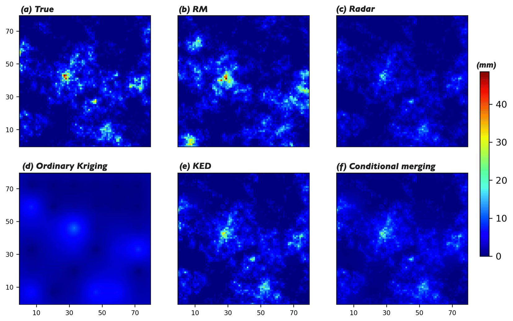
Figure 5(a) The true rainfall field; (b) a single realization from RM (scenario: G36, SNR = 3); (c) the radar estimates; (d–f) the estimates obtained from ordinary Kriging, Kriging with external drift (KED), and conditional merging, respectively.
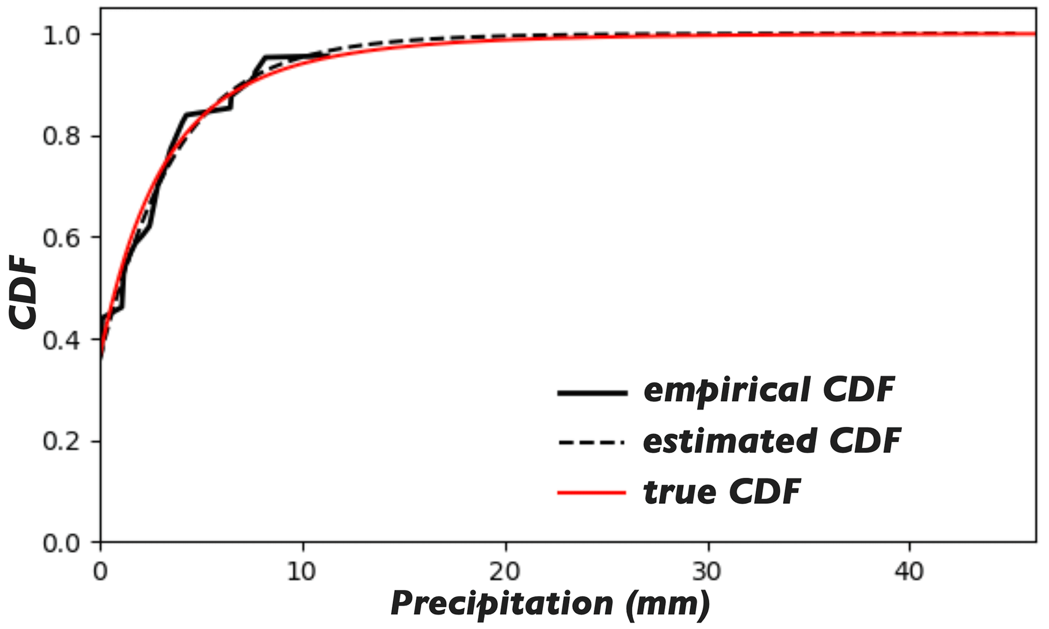
Figure 6The solid and dashed black lines show the empirical and estimated rainfall CDFs for the specific case shown in Fig. 5b. The red line shows the true rainfall CDF used in the generation of the true fields.

Figure 7(a) The true rainfall field; (b) the mean of 100 realizations obtained from RM (the small red dots denote the locations of the rain gauges, and the red triangles labelled with IDs denote the 9 px selected to develop the box and whisker plots shown in Fig. 8); (c) the standard deviation (std) of the 100 realizations.

4.1 Comparison of the results
The proposed approach (referred to simply as RM in this section, though RM is in fact only part of the approach) was used to estimate the 1000 true rainfall fields based on the corresponding radar estimates and rain gauge observations. The results from RM were compared with those from three well-known Kriging methods: ordinary Kriging, Kriging with external drift (KED), and conditional merging (Sinclair and Pegram, 2005). It is not possible to display all the results obtained in this paper; we focus on the results for one rainfall field randomly drawn from a total of 1000. A single realization obtained from RM is shown in Fig. 5b, which should be compared with the corresponding true rainfall field and the radar estimates presented in Fig. 5a and c, respectively. Meanwhile, the estimates obtained from ordinary Kriging, KED, and conditional merging are displayed in Fig. 5d–f, respectively. The results shown here are typical enough to be able to draw the following conclusions (conclusion 1 for ordinary Kriging, 2 for KED and conditional merging, and 3 for RM):
-
The rainfall field obtained from ordinary Kriging has neither the pattern nor the extremes of the true rainfall field, as the method only considers the rain gauge observations; the radar estimates do not contribute to the final estimates.
-
The estimates from KED and conditional merging capture the pattern but neither possess the extremes of the true field. KED outperforms conditional merging in this case because KED takes the radar estimates as the external drift and tries to capture the linear relationship between the gauge observations and the radar estimates at the gauge locations. Thus, the estimates from KED correct the extremes of the radar estimates a little bit but not perfectly, as radar underestimates the rainfall field nonlinearly in the scenario considered. In this specific case, the maximum values in the true and KED-estimated rainfall fields are 46.24 and 32.55 mm, respectively. Compared to KED, conditional merging is more dependent on the accuracy of the radar estimates, as the method assumes that the radar data provide an estimate of the actual Kriging error. As KED outperforms ordinary Kriging and conditional merging in this context, the results from RM are compared with those from KED in the following subsections.
-
The rainfall field obtained from RM captures the extremes of the true field. The maximum values in the true and RM-estimated rainfall fields are 46.24 and 47.57 mm, respectively. The pattern of the true field is captured with limited accuracy. After analysing the results from RM further, it is found that:
- 3.1.
The proposed approach is capable of capturing the extremes of the true field under the condition that the estimated rainfall CDF is relatively accurate; see the estimated and true CDFs for the specific case in Fig. 6.
- 3.2.
Unlike the estimates from ordinary Kriging, KED, or conditional merging, where one obtains a Kriged mean field, the proposed approach can yield an infinite number of realizations for the same true rainfall field due to the Monte Carlo framework. The mean of 100 realizations is displayed in Fig. 7b; this should be compared with the true rainfall field shown in Fig. 7a. From the figure, it can be seen that the mean realization is smooth and captures the pattern of the true field; in other words, the rain cells are more accurately located in the mean realization than in the individual realization. However, the statistics of the mean realization (variance and covariance) are clearly different from those of the true field. In summary, the individual realization gives relatively accurate statistics; an ensemble of such realizations is an accurate indicator of the locations of rainfall peaks. When feeding such an ensemble to applications such as a hydrological model, for example, one will also obtain an ensemble of estimates, meaning that the estimation uncertainty for the rainfall field will propagate.
- 3.3.
The various estimates from RM provide a reasonable representation of the estimation uncertainty. Figure 7c displays the standard deviation (std) of the 100 realizations. The black/zero-valued 6×6 pixels (which are uniformly distributed in the domain) reveal the locations of the rain gauges, as all the realizations present the same values at these locations. The exact locations of the rain gauges are marked by the small red dots in Fig. 7b. Compared to the Kriging variance, which reflects the relative positions of the unknowns and the data points only, the std map from RM is more physically meaningful. The estimation uncertainty of a pixel is affected by two factors: (a) the distance of the pixel from the data points (i.e. the uncertainty from the gauge side) and (b) the expected estimate at the pixel (i.e. the uncertainty from the radar side). There is a clear tendency: the closer the pixel to the neighbouring rain gauge and the smaller the expected estimate at the pixel, the lower the estimation uncertainty at the pixel.
To show the estimation uncertainty at different pixels, the box and whisker plots for nine selected pixels are displayed in Fig. 8. The locations and IDs of the nine pixels are given in Fig. 7b. It can be seen from the figure that the true values of the 9 px all fall in the central boxes, i.e. within the interquartile range (IQR). Among the 9 px, pixels 3, 4, and 8 are collocated with the rain gauges, and all the estimates at those 3 px equal the true values, which demonstrates the fulfilment of the equality constraints at the rain gauge locations directly. Pixels 1 and 2 are distant from their nearest rain gauges, but those two pixels are located in regions where less rainfall is expected. Thus, the estimates at the 2 px present relatively low variance. Pixels 5, 7, and 9 are also distant from their nearest rain gauges, but those 3 px are located in regions where more rainfall is expected. Thus, the corresponding estimates present higher variance. Though pixel 6 is close to its nearest rain gauge, it is located in a region where much rainfall is expected. Thus, the corresponding estimates show relatively high variance.
- 3.1.
4.2 Sensitivity analysis
The accuracy of the estimates is mainly affected by two factors: the number of rain gauge observations and the random error in the radar estimates. To analyse the influence of the two factors, the 1000 true rainfall fields were estimated under different scenarios: radar estimates with different levels of random error (SNR = 3, 5, and 10) and rain gauge networks with different layouts (5×5, 6×6, and 7×7 rain gauges that are uniformly distributed in the domain; these were denoted G25, G36, and G49, respectively). Specifically, we focus on two statistics when evaluating the estimation accuracy: the mean and maximum of the estimated rainfall field. The former is noteworthy when the estimated rainfall field is used in studies where the water balance of a region is important; the latter is of great importance when the extreme for the region is of interest (e.g. for stormwater management or flood risk assessment).

Figure 9Histograms of the errors w.r.t. the estimated field maxima for the 1000 true rainfall fields obtained by RM and KED. (a) The results for the scenarios with different rain gauge layouts, with the random error in the radar estimates fixed at SNR = 5. (b) The results for the scenarios with different levels of random error in the radar estimates, with the rain gauge layout fixed at G36.
4.2.1 Field maximum
The maximum of the rainfall field obtained from RM or KED is compared with the true maximum. Using RM, one could obtain an infinite number of realizations for each of the 1000 true rainfall fields, so we simulate an ensemble of 20 realizations for each true field and use the median of the 20 errors – the difference between the simulated and true maxima for each realization – as the representative. Figure 9 shows histograms of the errors w.r.t. the estimated field maxima for the 1000 fields obtained by RM and KED. Specifically, the upper panel shows the influence of the rain gauge layout and the lower panel shows the influence of the level of random error in the radar estimates. For the sake of clarity, we only display the scenarios with the most and least rain gauges (i.e. G25 and G49) in the upper panel, with the random error in the radar estimates fixed at SNR = 5. Similarly, in the lower panel, only the results of the scenarios with the largest and smallest levels of random error in the radar estimates (i.e. SNR = 3 and 10) are displayed, with the rain gauge layout fixed at G36. It can be seen from the figure that there are negative biases in all the results from KED, while the biases of the results from RM are not obvious. Further, it can be seen that increasing the number of rain gauges and reducing the level of random error in the radar estimates are both beneficial to the quality of the estimates, i.e. they reduce the size of the error and decrease the estimation variance (reduce the scatter in the histogram).
The histogram shown in Fig. 9 can be summarized by two statistics: the mean error (ME) and the interquartile range of the errors (IQR, the range between the quantiles 0.75 and 0.25). Table 1 shows the two statistics evaluated from the results for all the scenarios. It can be seen from the upper part of the table that the estimates from RM are slightly overestimated, and that the estimates from KED are significantly underestimated. For both methods, increasing the number of rain gauges and reducing the level of random error in the radar estimates help to reduce the ME and shrink the IQR. Yet for RM, more is not necessarily better. For example, the best performance in terms of ME and the best performance in terms of IQR both occur in scenario (SNR = 10, G36). Scenario (SNR = 10, G49) – which is assumed to perform the best – is only ranked second, possibly due to the overfitting problem in the estimation of the rainfall CDF. When the radar estimates are relatively accurate, the presence of a certain number of rain gauges is enough to sample sufficient information. Increasing the number of rain gauges further can lead to the overfitting problem, due to the surplus of information.

Figure 10Histograms of the errors w.r.t. the estimated field means for the 1000 true rainfall fields obtained by RM (a, b) and KED (c, d). The estimates were obtained under different scenarios; see the text in the subfigures for the specific scenarios.
Table 1The mean error (ME) and the interquartile range (IQR) of the errors w.r.t. the estimated field maxima for the 1000 true rainfall fields obtained by RM (the three columns on the left) and by KED (the three columns on the right). The column name denotes the SNR of the radar estimates whereas the row name denotes the rain gauge layout.
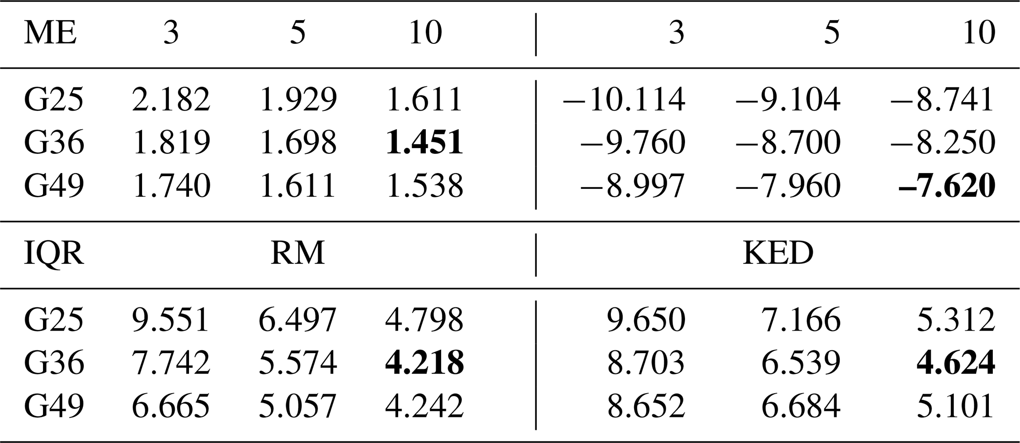
The best performances in terms of the ME and IQR for both methods are printed in bold.
4.2.2 Field mean
The estimated mean of the rainfall field by RM or KED is compared with the true mean to evaluate the accuracy in terms of the mean statistic. For each of the 1000 true fields, an ensemble of 20 realizations is produced by RM and the mean of the 20 errors – the difference between the simulated and the true means for each realization – is used as the representative. Figure 10 shows the histograms of the errors w.r.t. the estimated field means for the 1000 fields obtained from RM in Fig. 10a and b and from KED in Fig. 10c and d. It can be seen from the figure that, compared to RM, KED seems to be more sensitive to the two factors. Further, slight positive biases can be observed in the estimates from KED for all the displayed scenarios. Among the four subfigures, Fig. 10a and c show the influence of the rain gauge layout for RM and KED, respectively, while Fig. 10b and d show the influence of the level of random error in the radar estimates. For KED, the influences of the two factors are ambiguous. Increasing the number of rain gauges or reducing the level of random error in the radar estimates helps to reduce the estimation variance, but it is unclear whether it helps to reduce the size of the error. For RM, neither the influences of the two factors nor the biases in the estimates are obvious.
We still use the two statistics – ME and IQR – to generalize each histogram, and the results for all the scenarios are shown in Table 2. It can be seen from the upper part of the table that RM outperforms KED in terms of the ME, as the MEs from RM in all the scenarios are smaller than the best performance of KED. It is worth considering that, based on the previous analysis, KED is expected to underestimate the maximum of the rainfall field; however, the results shown here indicate that KED overestimates the mean of the field. KED is therefore likely to overestimate the lower quantiles of the rainfall field. Further, the table also demonstrates that RM is not very sensitive to the two factors in terms of the mean statistic, as one can see barely any trend.
Table 2The mean error (ME) and the interquartile range (IQR) of the errors w.r.t. the estimated field means for the 1000 true rainfall fields obtained by RM (the three columns on the left) and by KED (the three columns on the right). The column name refers to the SNR of the radar estimates, and the row name denotes the layout of the rain gauges.
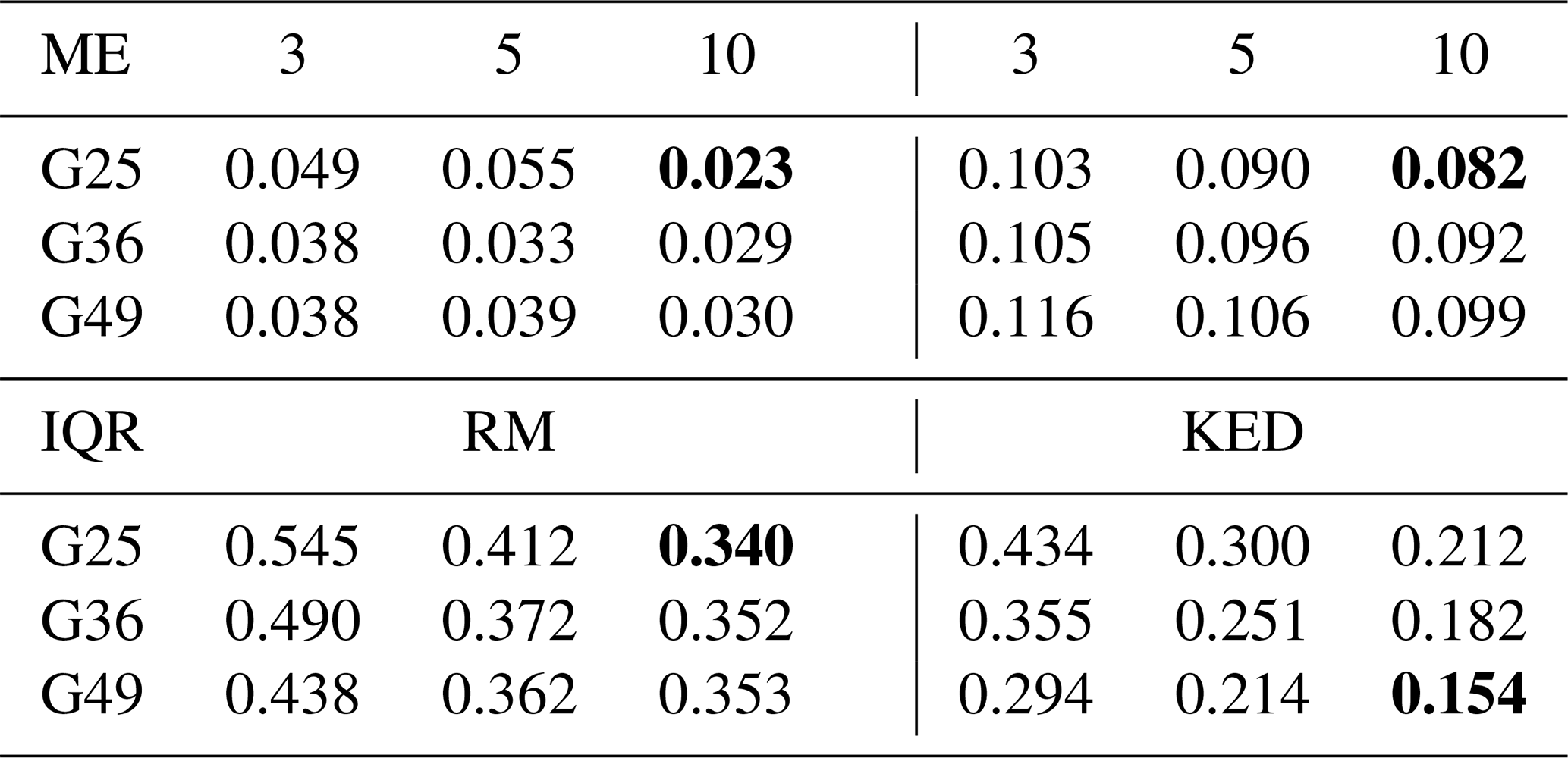
The best performance levels in terms of the ME and IQR for each method are printed in bold.
5.1 The two core components of the approach
In this paper, an approach allowing estimates of spatial rainfall fields to be obtained together with the associated uncertainty is proposed. This approach has two core components: the method used to compute the rainfall CDF (referred to as the CDF method hereafter) and the method of random mixing (RM), which is used to simulate random spatial fields under constraints.
The CDF method provides the foundation for the approach. A resultant rainfall CDF with sufficient accuracy is necessary for the successful application of the approach. The statistics of intermittent precipitation are not Gaussian, which restricts the usage of well-established stochastic models that assume Gaussianity (Pulkkinen et al., 2019). Specifically in this study, the rainfall CDF is important in two respects: (a) it is used in the data transformation, whereby the simulated Gaussian fields are transformed into rainfall fields of interest; (b) it is used to define the constraints in terms of the normalized Gaussian marginal.
RM, on the other hand, is an excellent tool that performs conditional simulation in Gaussian space, but it is not irreplaceable. Another conditional simulation method could have been used, such as phase annealing (Yan et al., 2020). RM was employed in this study due to (a) its relatively high efficiency, which makes the mass production of realizations possible, and (b) code availability (a Python package for the conditional simulation of random spatial fields using RM is available, with the authors giving practical demonstrations of the application of the method; Hörning and Haese (2021)).
5.2 The scope of the approach
The proposed approach is intended for the estimation of spatial rainfall fields following a short accumulation time: 15, 10, or even 5 min. The temporal aspects of QPE (quantitative precipitation estimates) are outside the scope of this study. Unlike the acquisition of QPF (quantitative precipitation forecasts) by e.g. a radar-based nowcast model when modelling the temporal evolution of the rainfall field is of interest, the spatial rainfall fields are obtained in a hindcast mode in this study. This approach has great potential to improve the quality of QPF. Shehu and Haberlandt (2020) showed that one of the major factors that causes the predictability loss of a nowcast model is the inability of radar to capture the true rainfall field. The proposed approach could therefore be used to improve the rainfall field fed into the model.
Furthermore, radar-based nowcasting has evolved from the use of a deterministic to the use of a probabilistic framework to estimate the predictive uncertainty (e.g. Pierce et al., 2012; Shehu and Haberlandt, 2020). A common approach is based on stochastic simulation, in which correlated noise fields are used to perturb a deterministic nowcast (e.g. Liguori and Rico-Ramirez, 2014; Foresti et al., 2016). The output of the proposed approach – an ensemble of estimates that considers both radar and rain gauge data – could be used to perturb a deterministic model, and this ensemble of estimates is more hydrologically meaningful than a random perturbation, which is used in many probabilistic nowcast models (e.g. Bowler et al., 2006; Berenguer et al., 2011; Pulkkinen et al., 2019). Besides, precipitation exhibits spatial variability; hence, it is challenging to estimate spatial rainfall fields in a deterministic manner, even in a hindcast mode. If the nowcasting community can embrace the change from a deterministic framework to a probabilistic one, a similar change could also happen in the hindcasting community.
5.3 Concerning the CDF method
5.3.1 Basic assumption
The rainfall CDF is computed from a set of rain gauge observations and the radar estimates. The basic assumption of the method is that the radar estimates can represent the pattern of the rainfall field to a reasonable extent. Random error, which can reduce the representativeness of the radar estimates, is accounted for, and the quality control steps in the algorithm are specifically designed to get rid of the negative effects of random error. However, the degradation of representativeness due to systematic effects in the radar estimates (e.g. range-dependent errors associated with the increasing height of the radar beam or increasing sampling volume as the distance from the radar antenna increases) is not accounted for. Thus, quality control to get rid of systematic effects in the radar estimates is necessary.
5.3.2 Impact of the distribution and number of rain gauge observations
The capability of the CDF method is affected by the distribution and number of rain gauge observations. A uniform distribution of rain gauge observations is not required, but the gauge observations should not be too clustered, as it is normally considered that one has a better chance of obtaining spatially representative samples from a relatively evenly distributed rain gauge network.
It is often the case that only small samples from irregularly distributed rain gauge stations are available for mesoscale hydrological studies. Sufficient gauge–radar pairs (samples) must be available if we are to obtain a rainfall CDF with adequate accuracy. There are two ways to increase the sample size:
-
Increase the sample size in space. For small domains with only a few rainfall stations (say 10), it can be assumed that rain parcels move uniformly. Under this assumption, one can displace the radar quantile map using a vector that decreases the radar–gauge mismatch (using the Spearman's rank correlation as the measure, for example) and then refind the gauge-respective quantiles in the displaced quantile map. The result is 10 new pairs (rk, ) for k=1, …, 10, where is the refound radar quantile. Normally, a stack of such vectors (N) can be found, which results in 10⋅N new samples. One should limit the domain size when applying the above practice. This technique has been applied by Yan and Bárdossy (2019) to find the empirical rainfall CDF for a domain of size 19×19 km2.
-
Increase the sample size in time. A fixed time window can be set by assuming a relatively stable distribution during the relevant time interval, and the gauge–radar pairs in the time window can be used in the calculation of the rainfall CDF.
A combination of both practices can enrich the sample size to a remarkable extent.
5.3.3 Impact of spatial intermittency
In this work, the performance of the CDF method was tested for the hydrologically interesting spatial intermittency u0=0.36. Practically speaking, the choice of u0 has only a minor influence on the performance. When u0>0.36 (i.e. a larger dry-area ratio), the point at which the rainfall CDF intersects the y axis moves up, and there are also more zero samples in both the radar and rain gauge data. When (i.e. a larger wet-area ratio), the point moves down and there are fewer zero samples. This method is problematic if u0=0, i.e. the entire domain is wet. In that case, there is no (0, u0) and the requirement (stated in step 4 in Sect. 2.1) that the CDF passes through the point (0, u0) does not apply.
5.3.4 Applicability in terms of the spatial scale
The CDF method is valid for a limited spatial scale. As the spatial scale increases, the domain eventually becomes too large for a single CDF to represent all processes. The limit on the spatial scale is related to factors such as rainfall regime, topography, and geography. However, because synthetic datasets were used instead of realistic datasets in this study, it was not possible to derive any useful information regarding the limit on the spatial scale. A further study based on realistic datasets is therefore required.
In this paper, an approach for simulating spatial rainfall fields conditioned on radar and rain gauge data was proposed. The approach has two core components: a method to compute the marginal distribution function of the rainfall field, and random mixing, which conducts a conditional simulation in Gaussian space. An artificial experiment was performed to test the efficiency of the proposed approach, and the results were compared with those from three commonly used Kriging methods: ordinary Kriging, Kriging with external drift (KED), and conditional merging. The proposed approach was found to outperform KED and conditional merging, especially in the estimation of extremes. The estimates yielded by the proposed approach differ from those provided by the other methods in two respects. First, unlike the Kriging methods, where a Kriged mean field is obtained by minimizing the estimation variance, the output of the approach is an ensemble of estimates (realizations) with identical statistics (mean, variance, correlation function, etc.) due to the Monte Carlo framework. Each individual realization strictly fulfils the equality constraints at rain gauge locations and presents a field pattern that is similar to the radar estimates, and an ensemble of such realizations provides a tendency towards the accurate locations of the rainfall peaks. Second, the various estimates from the proposed approach provide a reasonable representation of the estimation uncertainty. In addition to representing the relative positions of the unknowns and the data points (i.e. the information and the associated uncertainty from rain gauge data), which are also provided by the Kriging variance, the estimation uncertainty obtained with the proposed approach is more physically meaningful because the information and the associated uncertainty from radar data are also considered.
Further, the sensitivity of the proposed approach to the two factors – the number of rain gauges and the magnitude of the random error in the radar estimates – was analysed. We focused on the accuracy of the approach when estimating the maximum and the mean of the rainfall field, and the results were compared with those from KED. Concerning the estimation of the maximum, increasing the number of rain gauges and reducing the random error in the radar estimates help to improve the estimation quality. However, when the radar estimates are relatively accurate, a certain number of rain gauges are sufficient to sample adequate information on the rainfall field. Increasing the number of rain gauges further can lead to overfitting during the estimation of the rainfall CDF. Comparing the two methods, the proposed approach outperforms KED in terms of the mean error (ME) and the interquartile range (IQR) of the errors. Concerning the estimation of the mean, the proposed approach is not as sensitive as KED to the two factors. The proposed approach outperforms KED in terms of the ME, but the estimation variance is generally larger than that from KED.
In this paper, we presented a simulation study where synthetic rainfall fields were used as the true fields, and radar and rain gauge data used when applying the proposed approach were derived from those fields. Due to the full control over the stochastic process, it was possible to comprehensively examine the accuracy of the estimates based on the overall statistics and to analyse the sensitivity of the approach. However, there are several practical questions that cannot be answered without performing the relevant investigation based on realistic datasets. For example, explicit information on the largest spatial scale at which the CDF method can be reliably applied is required, and the effects of a small sample size and/or an irregular distribution of rain gauges on the performance of the approach remain interesting topics. Thus, further studies based on realistic datasets are necessary.
The datasets used when applying the proposed approach are available at https://doi.org/10.6084/m9.figshare.14864910.v1 (Yan, 2021). The generation procedures of the synthetic rainfall fields are explained in the Python script gen_gaugeData.py. The Python script gen_radar_gauge_data.py shows the generation procedures of the radar and rain gauge data. The Python script specsim_simple.py applies the method – fast Fourier transform for regular grids – to generate correlated Gaussian random fields.
The first author, JY, did the programming work and part of the manuscript writing. The first author, FL, did lots of computational work and part of the manuscript writing. They contributed equally to this work. The second author, AB, contributed to the research idea and supervised the research. The third author, TT, provided valuable suggestions for the revision of this article.
The authors declare that they have no conflict of interest.
Publisher’s note: Copernicus Publications remains neutral with regard to jurisdictional claims in published maps and institutional affiliations.
This research has been supported by the National Natural Science Foundation of China (grant nos. 04002340416, 51778452, and 51978493) and the China Postdoctoral Science Foundation (grant no. 0400229136).
This paper was edited by Nadav Peleg and reviewed by Scott Sinclair, Remko Uijlenhoet, and one anonymous referee.
Adams, T.: Chapter 10 – Flood Forecasting in the United States NOAA/National Weather Service, in: Flood Forecasting, edited by: Adams, T. E. and Pagano, T. C., Academic Press, Boston, 249–310, https://doi.org/10.1016/B978-0-12-801884-2.00010-4, 2016. a
Bárdossy, A. and Hörning, S.: Random Mixing: An Approach to Inverse Modeling for Groundwater Flow and Transport Problems, Trans. Porous Media, 114, 241–259, https://doi.org/10.1007/s11242-015-0608-4, 2016. a, b
Bell, T. L.: A space-time stochastic model of rainfall for satellite remote-sensing studies, J. Geophys. Res.-Atmos., 92, 9631–9643, https://doi.org/10.1029/JD092iD08p09631, 1987. a
Berenguer, M., Sempere-Torres, D., and Pegram, G.: SBMcast – An ensemble nowcasting technique to assess the uncertainty in rainfall forecasts by Lagrangian extrapolation, J. Hydrol., 404, 226–240, 2011. a
Berne, A. and Krajewski, W. F.: Radar for hydrology: Unfulfilled promise or unrecognized potential?, Adv. Water Resour., 51, 357–366, 2013. a
Bowler, N. E., Pierce, C. E., and Seed, A. W.: STEPS: A probabilistic precipitation forecasting scheme which merges an extrapolation nowcast with downscaled NWP, Q. J. Roy. Meteorol. Soc., 132, 2127–2155, https://doi.org/10.1256/qj.04.100, 2006. a
Brandes, E. A.: Optimizing Rainfall Estimates with the Aid of Radar, J. Appl. Meteorol., 14, 1339–1345, 1975. a
Calder, C. and Cressie, N.: Kriging and Variogram Models, in: International Encyclopedia of Human Geography, edited by: Kitchin, R. and Thrift, N., Elsevier, Oxford, 49–55, https://doi.org/10.1016/B978-008044910-4.00461-2, 2009. a
Chilès, J.-P. and Delfiner, P.: Geostatistics: Modeling Spatial Uncertainty, J. Am. Stat. Assoc., 95, 695, https://doi.org/10.1002/9781118136188, 2000. a
Collier, C.: The impact of wind drift on the utility of very high spatial resolution radar data over urban areas, Phys. Chem. Earth Pt. B, 24, 889–893, https://doi.org/10.1016/S1464-1909(99)00099-4, 1999. a
Crane, R. K.: Space-time structure of rain rate fields, J. Geophys. Res.-Atmos., 95, 2011–2020, 1990. a
Cristiano, E., ten Veldhuis, M.-C., and van de Giesen, N.: Spatial and temporal variability of rainfall and their effects on hydrological response in urban areas – a review, Hydrol. Earth Syst. Sci., 21, 3859–3878, https://doi.org/10.5194/hess-21-3859-2017, 2017. a
Curry, G. R.: Radar Essentials: A Concise Handbook for Radar Design and Performance Analysis, IET Digital Library, SciTech Publishing, https://doi.org/10.1049/SBRA029E, 2012. a
Deutsch, C. V. and Journel, A.: GSLIB – Geostatistical Software Library and User's Guide (Second edition), in: Applied Geostatistics Series, Oxford University Press, Oxford, https://doi.org/10.2307/1270548, 1998. a
Doviak, R. J. and Zrnić, D. S.: Doppler radar and weather observations, in: 2nd Edn., Academic Press, San Diego, 523–545, 1993. a
Emmanuel, I., Andrieu, H., Leblois, E., and Flahaut, B.: Temporal and spatial variability of rainfall at the urban hydrological scale, J. Hydrol., 430, 162–172, 2012. a
Fabry, F.: Radar meteorology: principles and practice, Cambridge University Press, Cambridge, 2015. a, b
Foresti, L., Reyniers, M., Seed, A., and Delobbe, L.: Development and verification of a real-time stochastic precipitation nowcasting system for urban hydrology in Belgium, Hydrol. Earth Syst. Sci., 20, 505–527, https://doi.org/10.5194/hess-20-505-2016, 2016. a
Haberlandt, U.: Geostatistical interpolation of hourly precipitation from rain gauges and radar for a large-scale extreme rainfall event, J. Hydrol., 332, 144–157, https://doi.org/10.1016/j.jhydrol.2006.06.028, 2007. a
Hengl, T., Heuvelink, G., and Stein, A.: Comparison of kriging with external drift and regression-kriging, Technical Note, ITC, available at: https://webapps.itc.utwente.nl/librarywww/papers_2003/misca/hengl_comparison.pdf (last access: June 2021), 2003. a
Hörning, S. and Haese, B.: RMWSPy (v 1.1): A Python code for spatial simulation and inversion for environmental applications, Environ. Model. Softw., 138, 104970, https://doi.org/10.1016/j.envsoft.2021.104970, 2021. a
Hu, L. Y.: Gradual deformation and iterative calibration of Gaussian-related stochastic models, Math. Geol., 32, 87–108, 2000. a, b, c
Hu, L. Y.: Combination of Dependent Realizations Within the Gradual Deformation Method, Math. Geol., 34, 953–963, https://doi.org/10.1023/A:1021316707087, 2002. a
Hu, L. Y., Blanc, G., and Noetinger, B.: Gradual Deformation and Iterative Calibration of Sequential Stochastic Simulations, Math. Geol., 33, 475–489, https://doi.org/10.1023/A:1011088913233, 2001. a
James, W. P., Robinson, C. G., and Bell, J. F.: Radar‐Assisted Real‐Time Flood Forecasting, J. Water Resour. Plan. Manage., 119, 32–44, 1993. a
Jiang, S., Ren, L., Hong, Y., Yong, B., Yang, X., Yuan, F., and Ma, M.: Comprehensive evaluation of multi-satellite precipitation products with a dense rain gauge network and optimally merging their simulated hydrological flows using the Bayesian model averaging method, J. Hydrol., 452–453, 213–225, https://doi.org/10.1016/j.jhydrol.2012.05.055, 2012. a
Kumar, P. and Foufoula-Georgiou, E.: Characterizing multiscale variability of zero intermittency in spatial rainfall, J. Appl. Meteorol., 33, 1516–1525, 1994. a
Lantuéjoul, C.: Geostatistical Simulation, J. Roy. Stat. Soc., 52, 699–700, 2002. a
Liguori, S. and Rico-Ramirez, M. A.: A review of current approaches to radar-based quantitative precipitation forecasts, Int. J. River Basin Manage., 12, 391–402, 2014. a
Liu, X., Yang, T., Hsu, K., Liu, C., and Sorooshian, S.: Evaluating the streamflow simulation capability of PERSIANN-CDR daily rainfall products in two river basins on the Tibetan Plateau, Hydrol. Earth Syst. Sci., 21, 169–181, https://doi.org/10.5194/hess-21-169-2017, 2017. a
Mantoglou, A. and Wilson, J. L.: The Turning Bands Method for simulation of random fields using line generation by a spectral method, Water Resour. Res., 18, 1379–1394, https://doi.org/10.1029/WR018i005p01379, 1982. a
Marshall, J. and Palmer, W.: The distribution of raindrops with size, J. Appl. Meteorol., 5, 165–166, https://doi.org/10.1175/1520-0469(1948)005<0165:TDORWS>2.0.CO;2, 1948. a
Méndez Antonio, B., Magaña, V., Caetano, E., da silveira, R., and Domínguez, R.: Analysis of daily precipitation based on weather radar information in México City, Atmosfera, 22, 299–313, 2009. a
Michaelides, S., Tymvios, F., and Michaelidou, T.: Spatial and temporal characteristics of the annual rainfall frequency distribution in Cyprus, Atmos. Res., 94, 606–615, https://doi.org/10.1016/j.atmosres.2009.04.008, 2009. a
Michelson, D. B. and Koistinen, J.: Gauge-radar network adjustment for the Baltic Sea Experiment, Phys. Chem. Earth Pt. B, 25, 915–920, 2000. a
Pegram, G. G. and Clothier, A. N.: High resolution space-time modelling of rainfall: the “String of Beads” model, J. Hydrol., 241, 26–41, https://doi.org/10.1016/S0022-1694(00)00373-5, 2001. a
Pierce, C., Seed, A., Ballard, S., Simonin, D., and Li, Z.: Nowcasting, in: Doppler Radar Observations – Weather Radar, Wind Profiler, Ionospheric Radar, and Other Advanced Applications, edited by: Bech, J. and Chau, J. L., InTech, 97–142, https://doi.org/10.5772/39054, 2012. a
Pulkkinen, S., Nerini, D., Pérez Hortal, A. A., Velasco-Forero, C., Seed, A., Germann, U., and Foresti, L.: Pysteps: an open-source Python library for probabilistic precipitation nowcasting (v1.0), Geosci. Model Dev., 12, 4185–4219, https://doi.org/10.5194/gmd-12-4185-2019, 2019. a, b
Ravalec, M. L., Noetinger, B., and Hu, L. Y.: The FFT Moving Average (FFT-MA) Generator: An Efficient Numerical Method for Generating and Conditioning Gaussian Simulations, Math. Geol., 32, 701–723, https://doi.org/10.1023/A:1007542406333, 2000. a
Schuurmans, J. M., Bierkens, M. F. P., Pebesma, E. J., and Uijlenhoet, R.: Automatic Prediction of High-Resolution Daily Rainfall Fields for Multiple Extents: The Potential of Operational Radar, J. Hydrometeorol., 8, 1204–1224, https://doi.org/10.1175/2007JHM792.1, 2007. a
Shehu, B. and Haberlandt, U.: Relevance Of Merging Radar And Rainfall Gauge Data For Rainfall Nowcasting In Urban Hydrology, J. Hydrol., 594, 125931, https://doi.org/10.1016/j.jhydrol.2020.125931, 2020. a, b, c
Sideris, I., Gabella, M., Erdin, R., and Germann, U.: Real-time radar–raingauge merging using spatio-temporal co-kriging with external drift in the Alpine terrain of Switzerland, Q. J. Roy. Meteorol. Soc., 140, 1097–1111, https://doi.org/10.1002/qj.2188, 2014. a
Sinclair, S. and Pegram, G.: Combining radar and rain gauge rainfall estimates using conditional merging, Atmos. Sci. Lett., 6, 19–22, https://doi.org/10.1002/asl.85, 2005. a, b
Todini, E.: A Bayesian technique for conditioning radar precipitation estimates to rain-gauge measurements, Hydrol. Earth Syst. Sci., 5, 187–199, https://doi.org/10.5194/hess-5-187-2001, 2001. a
Uijlenhoet, R.: Raindrop size distributions and radar reflectivity–rain rate relationships for radar hydrology, Hydrol. Earth Syst. Sci., 5, 615–628, https://doi.org/10.5194/hess-5-615-2001, 2001. a
Velasco-Forero, C. A., Sempere-Torres, D., Cassiraga, E. F., and Gómez-Hernández, J. J.: A non-parametric automatic blending methodology to estimate rainfall fields from rain gauge and radar data, Adv. Water Resour., 32, 986–1002, https://doi.org/10.1016/j.advwatres.2008.10.004, 2009. a
Verworn, A. and Haberlandt, U.: Spatial interpolation of hourly rainfall – effect of additional information, variogram inference and storm properties, Hydrol. Earth Syst. Sci., 15, 569–584, https://doi.org/10.5194/hess-15-569-2011, 2011. a
Wang, L. P., Ochoa-Rodriguez, S., Simões, N., Onof, C., and Maksimovic, Č.: Radar-raingauge data combination techniques: A revision and analysis of their suitability for urban hydrology, Water Sci. Technol., 68, 737–47, 2013. a
Wilson, J. W.: Integration of Radar and Raingage Data for Improved Rainfall Measurement, J. Appl. Meteorol., 9, 489–497, https://doi.org/10.1175/1520-0450(1970)009<0489:IORARD>2.0.CO;2, 1970. a
Wood, A. T.: When is a truncated covariance function on the line a covariance function on the circle?, Stat. Probab. Lett. 24, 157–164, https://doi.org/10.1016/0167-7152(94)00162-2, 1995. a
Wood, A. T. and Chan, G.: Simulation of stationary Gaussian processes in [0, 1] d, J. Comput. Graph. Stat., 3, 409–432, 1994. a
Yan, J.: Supplementary material for the paper “Conditional simulation of spatial rainfall fields using random mixing: a study that implements full control over the stochastic process”, Figshare, https://doi.org/10.6084/m9.figshare.14864910.v1, 2021. a
Yan, J. and Bárdossy, A.: Short time precipitation estimation using weather radar and surface observations: With rainfall displacement information integrated in a stochastic manner, J. Hydrol., 574, 672–682, https://doi.org/10.1016/j.jhydrol.2019.04.061, 2019. a
Yan, J., Bárdossy, A., Hörning, S., and Tao, T.: Conditional simulation of surface rainfall fields using modified phase annealing, Hydrol. Earth Syst. Sci., 24, 2287–2301, https://doi.org/10.5194/hess-24-2287-2020, 2020. a, b
Yilmaz, K. K., Hogue, T. S., Hsu, K.-L., Sorooshian, S., Gupta, H. V., and Wagener, T.: Intercomparison of Rain Gauge, Radar, and Satellite-Based Precipitation Estimates with Emphasis on Hydrologic Forecasting, J. Hydrometeorol., 6, 497–517, https://doi.org/10.1175/JHM431.1, 2005. a