the Creative Commons Attribution 4.0 License.
the Creative Commons Attribution 4.0 License.
 | 30 Jun 2021
Time lags of nitrate, chloride, and tritium in streams assessed by dynamic groundwater flow tracking in a lowland landscape
Vince P. Kaandorp
Hans Peter Broers
Ype van der Velde
Joachim Rozemeijer
Perry G. B. de Louw
Surface waters are under pressure from diffuse pollution from agricultural activities, and groundwater is known to be a connection between the agricultural fields and streams. This paper is one of the first to calculate long-term in-stream concentrations of tritium, chloride, and nitrate using dynamic groundwater travel time distributions (TTDs) derived from a distributed, transient, 3D groundwater flow model using forward particle tracking. We tested our approach in the Springendalse Beek catchment, a lowland stream in the east of the Netherlands, for which we collected a long time series of chloride and nitrate concentrations (1969–2018). The Netherlands experienced a sharp decrease in concentrations of solutes leaching to groundwater in the 1980s due to legislations on the application of nitrogen to agricultural fields. Stream measurements of chloride and nitrate showed that the corresponding trend reversal in the groundwater-fed stream occurred after a time lag of 5–10 years. By combining calculated TTDs with the known history of nitrogen and chloride inputs, we found that the variable contribution of different groundwater flow paths to stream water quality reasonably explained the majority of long-term and seasonal variation in the measured stream nitrate concentrations. However, combining only TTDs and inputs underestimated the time lag between the peak in nitrogen input and the following trend reversal of nitrate in the stream. This feature was further investigated through an exploration of the model behaviour under different scenarios. A time lag of several years, and up to decades, can occur due to (1) a thick unsaturated zone adding a certain travel time, (2) persistent organic matter with a slow release of N in the unsaturated zone, (3) a long mean travel time (MTT) compared to the rate of the reduction in nitrogen application, (4) areas with a high application of nitrogen (agricultural fields) being located further away from the stream or drainage network, or (5) a higher presence of nitrate attenuating processes close to the stream or drainage network compared to the rest of the catchment. By making the connection between dynamic groundwater travel time distributions and in-stream concentration measurements, we provide a method for validating the travel time approach and make the step towards application in water quality modelling and management.
- Article
(5529 KB) - Full-text XML
- BibTeX
- EndNote


Diffuse pollution with nutrients is one of the main pressures on Europe's surface- and groundwaters (EEA, 2018). Intensive agricultural land use and the accompanying use of manure and fertilizers have significantly increased the amount of nitrate in the hydrological system in the period after 1950 (Aquilina et al., 2012; Broers and van der Grift, 2004; Hansen et al., 2011; Worrall et al., 2015). From 1985, nitrate concentrations leaching towards the groundwater decreased as a result of national and European legislations (Dutch Manure Law, 1986; EU Nitrates Directive, 1991) that contain rules for the reduction of N applications in farming. The following trend reversal in the concentrations of surface waters has been reported in few countries, including the Netherlands (e.g. van den Brink et al., 2008; Visser et al., 2007; Zhang et al., 2013; Rozemeijer et al., 2014) and Denmark (Hansen et al., 2011).
Land use determines the timing and quantity of nitrate input and its spatial distribution (Boumans et al., 2008). For example, the input of nutrients is higher on fertilized agricultural fields than in forested areas. Nitrate leaches to the groundwater (Boumans et al., 2008; Wang et al., 2012) on locations with different land uses and distances to the stream, from where it is transported towards the streams through fast and slow groundwater flow paths. These flow paths reach certain depths and cross different geological formations, taking a certain travel time from infiltration to exfiltration (Broers and van Geer, 2005; Howden et al., 2011b; van der Velde et al., 2010). Groundwater flow paths spatially connect infiltration areas and in-stream seepage zones (e.g. Ali et al., 2014; Birkel et al., 2015; McGuire and McDonnell, 2010). Groundwater flow paths also temporally connect changes in solute leaching, for example, due to land use changes with a response in stream water concentrations that may occur many years later (e.g. Van Meter and Basu, 2017). Both flow paths and travel times also influence hydrochemical processes, as they determine which media are passed and the time that is available for (biogeo)chemical reactions. Nitrate concentrations may, for instance, decrease by denitrification when passing organic or pyrite-rich layers (e.g. Zhang et al., 2013). Consequently, all water particles may carry different nitrate concentrations depending on their place and time of infiltration, their flow paths, and their travel times along their flow paths. Because groundwater flow path contributions to stream discharge are dynamic throughout the year, with activation or deactivation and changes in outflow locations, the delivery of nitrate from groundwater to surface waters also varies in time (Rozemeijer and Broers, 2007). Groundwater flow paths and travel times are thus an important control on the mean and variance of nitrate concentrations in groundwater and streams both in time and space (e.g. Musolff et al., 2017). Although much research on flow paths and travel times has been done, the reasons for observed time lags between a decrease in solute input and the following trend reversal in stream concentrations are not yet fully known.
To understand the source of observed and predicted future stream water quality trends, a model of groundwater flow paths is essential. Such models can be implicit (e.g. Benettin et al., 2017; Harman, 2015; Hrachowitz et al., 2009; van der Velde et al., 2010), using the inherent averaging properties of stream discharge as the sum of all flow paths within a catchment to justify simplifying a catchment into a single reservoir, or several reservoirs, with average inputs and reactions. Many of the spatially implicit approaches for catchment-scale transport of solutes rely on travel time. Despite that stream travel times cannot (yet) be measured directly, travel times are strongly constrained by the catchment water balance. Several studies have found strong correlations between the distribution of travel times in a stream and the solute concentrations in that stream (Hrachowitz et al., 2009; van der Velde et al., 2010). The disadvantage of using implicit, travel-time-based approaches is that spatial features, such as organic or pyrite-rich layers (e.g. Lutz et al., 2020; Zhang et al., 2013) that cause denitrification, or local sources of high inputs, which can strongly affect stream nitrate concentration and dynamics, often remain unnoticed in the implicit modelling results. Contrary to the implicit models, explicit models do consider these features. Explicit models describe all water flows from infiltration to exfiltration (e.g. Kaandorp et al., 2018a; Yang et al., 2018) and take into account location-specific source inputs, subsurface hydraulic properties, and subsurface reactivity.
In a recent paper, Kaandorp et al. (2018a) presented an explicit modelling approach for lowland catchments in the Netherlands. Using a groundwater model and particle tracking, they calculated dynamic travel time distributions (TTDs) and showed how groundwater flow path contributions in these catchments vary in time. From this, they discussed differences in mixing processes between young and old groundwater in the streams with time. In this follow-up paper, we used these previously calculated dynamic travel time distributions and the accompanying spatially explicit groundwater flow paths to explore the potential reasons for time lags in agricultural contaminants delivery towards a stream. For this purpose, we added the transport of tritium, chloride, and nitrate towards the stream and compared simulated with observed concentrations in the Dutch Springendalse Beek stream from 1969 until the present. We chose tritium because it is part of the actual water molecule and thus a good tracer of water itself, chloride because it is considered to be a conservative tracer of manure and fertilizers when it passes through the aquifer, and nitrate because it is a problem solute that causes eutrophication of downstream waters. In our study, tritium, chloride, and nitrate were measured. This work extends on recent advances in research on the groundwater contribution to streams (e.g. Engdahl et al., 2016; McDonnell et al., 2010; Morgenstern et al., 2010; Solomon et al., 2015; van der Velde et al., 2012) and is one of the first to couple measurement data of water quality and isotopes to dynamic TTDs and flow path dynamics calculated with a forward particle tracking model. Even though many recent papers suggest that this method holds a lot of potential (e.g. Hrachowitz et al., 2016), the papers which have attempted to do so are still scarce due to a lack of long-term solute input in the range of 5–50 years and discharge concentration data. Subsequently, we exploit the strong physical basis of particle-based flow paths to explore the controls on time lags in the breakthrough of agricultural nitrate, such as biogeochemical legacy effects, denitrification in soils and groundwater, management options, and differences in the spatial input patterns.
Our aims of this study are twofold. First, we aim to corroborate the simulated flow paths with measured tritium and chloride concentrations and, second, to explore the effect of different processes and parameter values and spatial input patterns on the simulated breakthrough patterns, trend reversals, and time lags between input and stream discharge for both chloride and nitrate. With this approach, we sketch a way forward in (a) modelling of groundwater-fed catchments and (b) management of (ground)watersheds.
2.1 Study area
A lowland stream in the east of the Netherlands, the Springendalse Beek (Fig. 1), was selected for this study because of its high nitrate concentrations and differences in land use and discharge characteristics between upstream and downstream parts of the catchment (Kaandorp et al., 2018b). The catchment has a temperate marine climate with a mean temperature of 9.6 ∘C and mean annual precipitation and evaporation of around 850 and 560 mm respectively. The size of the catchment is 4 km2, and the average discharge downstream is 0.043 m3 s−1, with a baseflow index of 0.8 (Gustard et al., 1992).
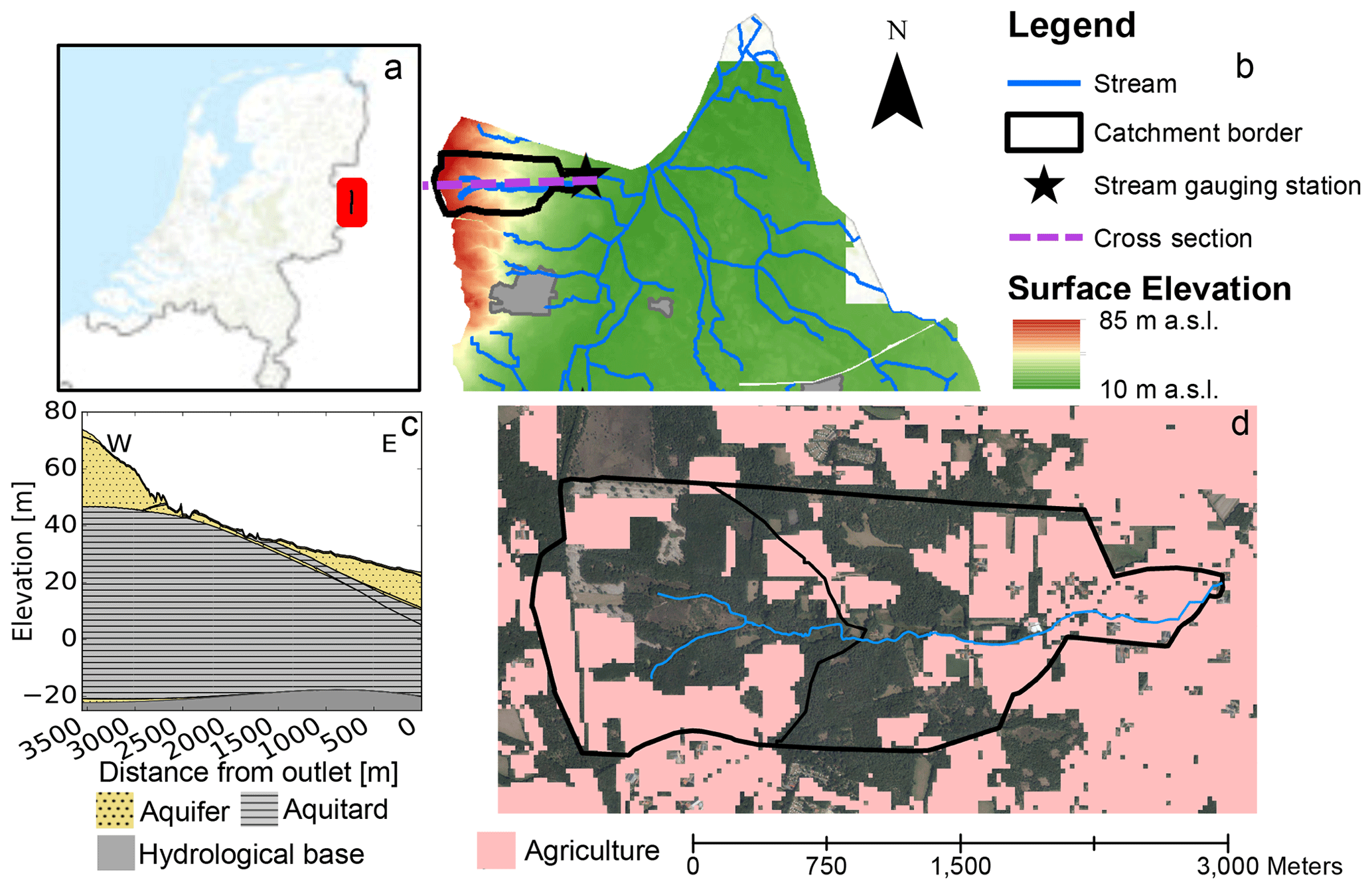
Figure 1Location of the study area (a, b), model conceptualization (c), and the location of agricultural fields in the year 2007 (d). Background maps and digital elevation model (DEM) are from PDOK (Public Services on the Map; https://www.pdok.nl/datasets, last access: 21 March 2019).
The catchment is located on the flank of an ice-pushed ridge that was formed during the Saalian glaciation and has a maximum elevation of 75 m a.s.l. (above sea level). Recent hydrogeological inventories suggest a complex ice-pushed structure composed of a series of tilted slabs of Tertiary clays (Breda Formation and older) intercalated with Pleistocene moderately coarse, organic-poor sands, and some gravel that was deposited by a braided river (Appelscha Formation). These slabs roughly have a N–S strike direction, perpendicular to the receiving Springendalse Beek stream (Ronald Harting and Marcel Bakker, TNO Geological Survey of the Netherlands, personal communication, 2019) and can hardly be passed by groundwater flow, leading to relatively high groundwater tables compared to more sandy ice-pushed ridges in the Netherlands. In general, the average depth of the water table is around 0.5 m below the surface in the downstream part of the catchment and up to about 3 m below the surface in the highest parts of the upstream catchment, presumably concentrated at outcrops of the Pleistocene sands.
The upstream part (2 km2) of the Springendalse Beek catchment has several spring areas and is mostly forested with some agricultural fields, while farmland is more abundant in the downstream part (2 km2) of the catchment. Many of these farmlands are artificially drained by a system of tile drains and ditches, especially in the downstream part of the catchment, due to the flatter topography and more shallow groundwater tables compared to the upstream part of the catchment. Available data indicate that the drainage density is around 20 %–30 % lower in the upstream part of the catchment than in the downstream part. Due to its constant flow and permanent springs, the stream is known to have a high ecological value (e.g. Nijboer et al., 2003; Verdonschot et al., 2002).
2.2 Collecting water quality measurements of surface water
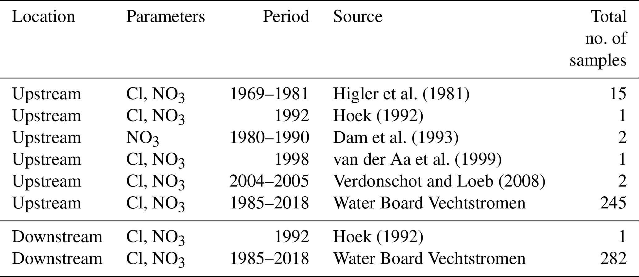
Surface water quality measurements were collected from various sources (Table 1), with a focus on the availability of data on chloride and nitrate. First, historical data, from 1969 onwards, of chloride and nitrate concentrations was obtained from earlier studies (Dam et al., 1993; Higler et al., 1981; Hoek, 1992; van der Aa et al., 1999; Verdonschot and Loeb, 2008). This data set was complemented with a 1985–present time series of chloride and nitrate that was collected by the monitoring programme of the local Water Board Vechtstromen. In addition, we started sampling for 3H in 2016 because we anticipated that tritium could give an independent validation of our transient TTD model. In total, 10 samples were taken over the period 2016 to 2018. These were stored in 1 L plastic containers and measured at the Bremen mass spectrometric facility by degassing followed by analysis of 3He with a sector field mass spectrometer (MAP 215-50; Sültenfuß et al., 2009).
Table 1Overview of the collected chloride and nitrate measurements.
2.3 Groundwater model and TTDs
Backward travel time distributions (TTDs) describe the distribution of ages of the water that contributes to discharge in a catchment. Dynamic TTDs do this in a time-variable way and show, for instance, seasonality in the contribution of older and younger water. Dynamic TTDs for the Springendalse Beek catchment were calculated using forward particle tracking on a high-resolution spatially distributed groundwater flow model following the method described by Kaandorp et al. (2018a). Groundwater flow was calculated using an existing finite difference groundwater flow model (MODFLOW; Harbaugh, 2005) created and calibrated on groundwater heads and validated with both groundwater heads and river discharge in earlier studies (Hendriks et al., 2014; Kuijper et al., 2012). Groundwater flow was simulated with a monthly time step on a regional scale (total modelled area 58 km by 45 km) with cells of 25×25 m. The top of the model followed the surface elevation, and the model consisted of seven layers of variable thickness, based on the Dutch Geohydrological Information System (REGIS II, 2005). Figure 1 gives a 2D cross section through the model's hydrogeological schematization of the subsurface, which is a gross simplification typical in regional groundwater flow models. Mean aquifer thickness in the model was approximately 18 m but varied between 0.5 and 30 m. Transmissivity in the aquifers was approximately 40 m2 d−1, porosity was assumed to be 0.3 m3 m−3, and some anisotropy was added in the ice-pushed ridges (Kuijper et al., 2012). The entire drainage system in the catchment was modelled using the Drain (DRN) and River (RIV) MODFLOW packages (Harbaugh, 2005). Flow through the unsaturated zone was modelled using the MetaSWAP model for a seasonal representation of the groundwater recharge (De Lange et al., 2014; van Walsum and Groenendijk, 2008; van Walsum and Veldhuizen, 2011). This unsaturated-zone model consists of soil column models and uses soil physical relationships to calculate water content profiles and water balances. It includes the calculation of actual evaporation and transpiration based on land use and vegetation type and considers evapo(transpi)ration from groundwater. The groundwater and particle tracking model was run for the period of 1700–2017 to allow for the calculation of long groundwater flow paths, repeating climate data from the period 1965–2017 (see Kaandorp et al., 2018a).
Groundwater travel times (TTs), representing the age of the water that contributes to streamflow (Benettin et al., 2015; Harman, 2015; van der Velde et al., 2012), were calculated using a combination of forward particle tracking and volume book keeping (Kaandorp et al., 2018a). Using the flow velocities calculated by the groundwater flow model, particle tracking software MODPATH version 3 (Pollock, 1994) was used to calculate transient flow paths and TTs. Particles were released monthly at the water table at the centre of each model cell and represented the volume equal to the total groundwater recharge of that month. Particles were released for the total model period spanning 317 years, yielding a total of 3804 particle tracking runs with around 14 000 particles each. Particles were stopped at sinks, such as wells, rivers, or drains (Visser et al., 2009), when the fraction of discharge to the sink was larger than 50 % of the total inflow to the cell (see also Kaandorp et al., 2018a). To construct monthly TTDs, particles were collected on a monthly timescale at their end points in an area of interest (whole catchment or part of catchment).
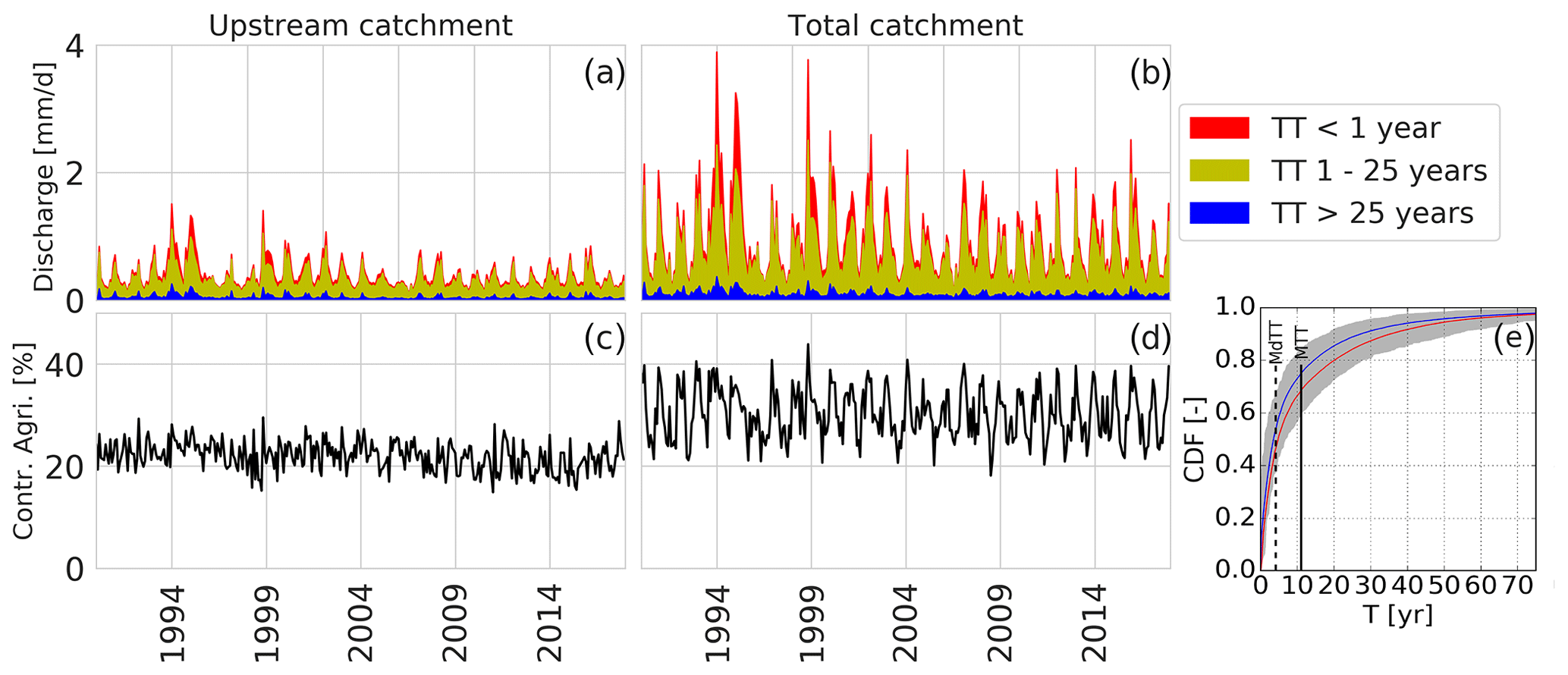
Figure 2The three age classes of the travel time distributions of the discharge in the Springendalse Beek for the upstream part of the catchment (a) and the total catchment (b). The lower panels show the percentage of discharge originating from agricultural fields for the upstream part of the catchment (c) and the total catchment (d). Panel (e) shows the time-weighted averaged cumulative distribution function (CDF) of the travel time distributions of the total catchment in summer (red) and winter (blue) and the overall median and mean TTs.
Using this model approach, Kaandorp et al. (2018a) showed travel time distributions, with an exponential-like shape, with a mean travel time of approximately 11 years and a median travel time of around 4 years. About 20 % of discharge in the Springendalse Beek is water with a travel time of less than 1 year, while about 15 % of discharge has a travel time of more than 25 years (Fig. 2a and b). The discharge in the Springendalse Beek thus consists mainly of medium-aged water (1–25 years). Based on the land use map (Fig. 1) and the particle tracking, between 15 % and 25 % of discharge infiltrated under agricultural fields in the upstream part of the catchment (Fig. 2c). For the total catchment, this is slightly higher, at about 25 % to 35 % (Fig. 2d), because a slightly larger part of the stream's capture zone in the downstream part of the catchment is used for agriculture. In the modelling results, the discharge contribution from agricultural fields shows a seasonal pattern especially for the total catchment (Fig. 2d), with a higher contribution to discharge of water that was infiltrated under agricultural fields during the wet winter. Interestingly, the mean travel time from agricultural fields is approximately 13 years in the upstream catchment compared to 11 years for the total catchment (median TT 8 years vs. 4 years).
The modelling assumptions and simplifications that were made have some drawbacks. As we started the particles at the water table, we effectively neglected the travel time through the unsaturated zone (e.g. Green et al., 2018; Sprenger et al., 2016; Wang et al., 2012), but this layer was generally thin in the study area (mostly <1 m) and is partly bypassed by preferential flow. Because particles were released monthly at the centre of each model cell, short travel times (<1 month) were not included at all, and particles had to travel at least 12.5 m before reaching a next cell, causing further uncertainty to short travel times. Several processes were not included in the modelling approach, such as overland flow and re-infiltration of seeped water. Overland flow is not an important flow route in the catchment on a yearly basis, and nitrate concentrations in overland flow are low due to little interaction with the soil. This paper thus focusses on longer groundwater TTs and timescales (>1 month). Chemical processes in the unsaturated zone concerning nitrate were included in constructing the solute input time series.
2.4 Tritium input time series
In principal, a series of tritium measurements in streams can be used to derive (ground)water age distributions (Broers and van Vliet, 2018a; Cartwright and Morgenstern, 2015; Duvert et al., 2016; Gusyev et al., 2014; Morgenstern et al., 2010; Solomon et al., 2015; Stewart et al., 2017). Here, we intend to use 3H in an opposite approach by validating our dynamic groundwater model TTDs using a short series of 3H measurements in the gaining stream (as e.g. Rodriguez et al., 2020). For the 3H input into our model, we combined the monthly measurements of tritium in precipitation of the closest measurement stations at Groningen (1970–2010) and Emmerich (1978–2016; the distance from the catchment to these stations is 80 to 90 km) taken from the Global Network of Isotopes in Precipitation (GNIP) database of tritium activity in precipitation (IAEA/WMO, 2018). For months that both stations had measurements, we used the average concentration, as our study area is located approximately halfway between these two measurement stations. For months that measurements from both stations were not available, we adjusted the available data using a factor based on the average difference between the stations, following an approach similar to Meinardi (1994). Because the relation between the values measured at the two stations changes in time, we use two factors. Before 1997, we used Emmerich equal to Groningen × 1.49. From 1997 onwards, we used Emmerich equal to Groningen × 1.03. For the period before 1970, we used adjusted measurements from Vienna and Ottawa, roughly following Meinardi (1994).
2.5 Land use and input time series for N and Cl
We distinguished two types of land use, namely farmlands and natural vegetation, which include forests and heather (Fig. 1). Concentrations of solutes reaching the water table below natural areas were assumed to be constant in time, i.e. 15 mg L−1 for chloride and 5 mg L−1 for nitrate, which are conservative estimates based on Kros et al. (2004) and Van Beek et al. (1994). Although these concentrations of solutes have not been constant during the last decades (e.g. Boumans et al., 2013), we feel that this assumption is acceptable as the concentration changes due to atmospheric deposition are much smaller than those due to agricultural inputs. For agricultural fields, a solute input time series was constructed on an annual basis. For the period 2000 to 2017, we used the data from the Dutch sandy areas of the Dutch Minerals Policy Monitoring Programme (LMM), which includes monitored concentrations in the uppermost first metre below the water table at agricultural fields since 1991 (see e.g. Boumans et al., 2005; Fraters et al., 2015). For the period 1950 to 2000, we used the nitrogen (N) and chloride surplus that was derived from historical bookkeeping records of minerals applied to farmlands and corrected for crop uptake (Broers and van der Grift, 2004; van den Brink et al., 2008; Visser et al., 2007). We combined this data with the 2000–2017 LMM data by fitting the overlap between 1991–2000 by adjusting the older data to correspond to a groundwater recharge of 0.35 m yr−1, and to represent (part of) the nitrate transformation processes in the unsaturated zone, we used a nitrate transformation factor of 0.85. This factor represents an average nitrate denitrification in the unsaturated zone and the value used here corresponds with Dutch data for soils with average water tables around 1 m depth (Steenvoorden et al., 1997; van den Brink et al., 2008). Land use change was considered for an agricultural field of approximately 7.5 ha (∼2 %) that was converted to natural vegetation in 1998. What was not considered is that small parts of the catchment changed from nature to agriculture and vice versa. This does not have a large effect on the downstream surface water concentrations.
2.6 Water quality modelling
The calculated dynamic TTDs were combined with the input time series of solutes to create a water quality model. Thus, tritium, chloride, and nitrate inputs were assigned to the particles based on their starting time and location (natural or agricultural). Figure 1 shows the areas where the constructed agricultural input time series was used as input for the model, and the other parts of the catchments were given the constant concentration of natural vegetation (see Sect. 2.5). In a similar way as in the construction of the TTDs (Kaandorp et al., 2018a), particles that contributed to stream discharge were combined for each month, and their concentrations were weighted based on their volumes to simulate the concentrations in the stream. The input concentrations of chloride and nitrate were assumed constant over a specific year, whereas monthly 3H measurements were directly assigned to the particles in the starting month. The model keeps track of particles that are lost through evapo(transpi)ration, thus effectively removing water and 3H in periods of a precipitation deficit. For chloride and nitrate, the solute input is constant over the year, and based on concentrations in the uppermost groundwater, thus there is no need to further account for evapo(transpi)ration for these solutes.
In the initial water quality model run, no chemical processes, such as denitrification, were implemented. Thus, in this model run the calculated stream solute concentrations are only based on the input time series and groundwater travel time. We did not intend to add further local details to improve the model performance; instead, we aimed at understanding the hydrological and hydrochemical processes relevant for time lags between the application of solutes and discharge in the stream, which is also useful outside our study catchment. Thus, we explored the model behaviour under different scenarios of chemical and hydrological processes.
2.7 Exploration of the model behaviour under different scenarios
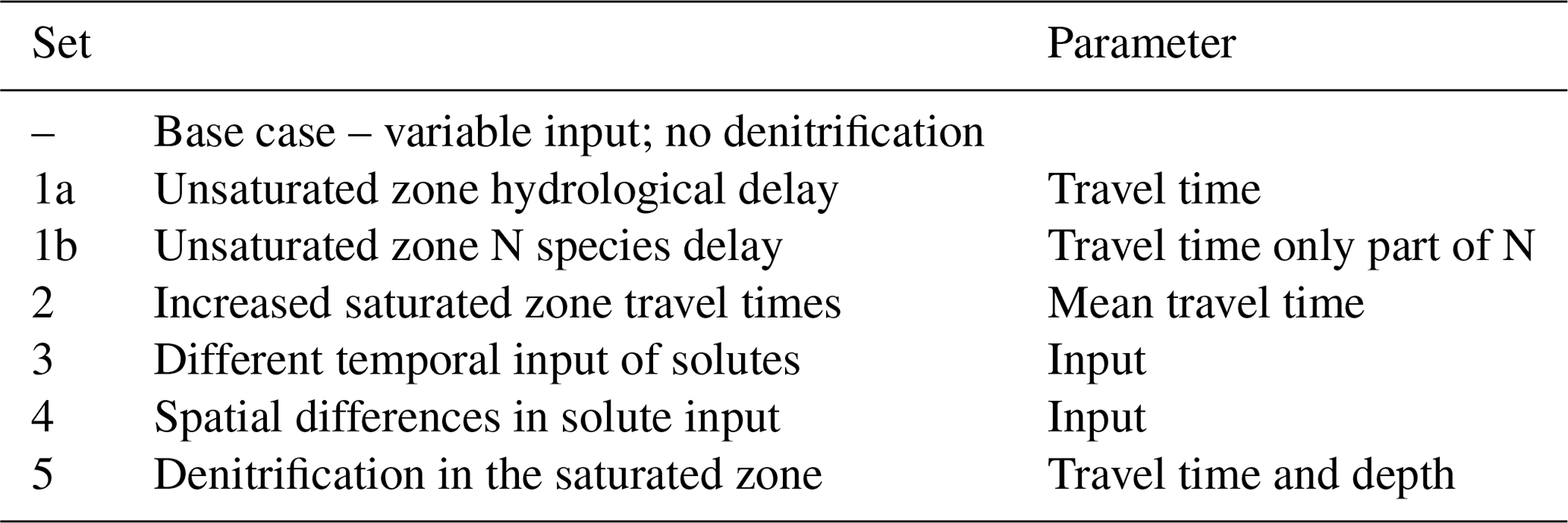
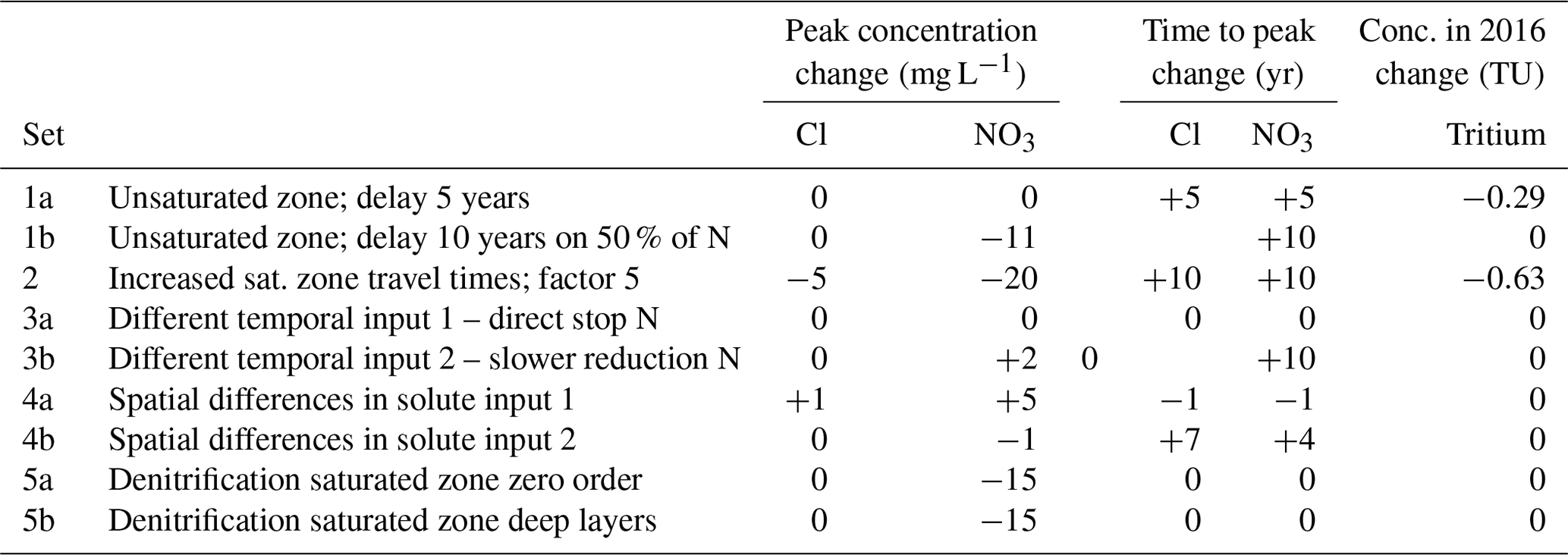
The initial run of the water quality model was only based on the constructed solute input time series and the dynamic TTDs derived from the calibrated groundwater flow model. In this model run, the spatial distribution of solute input (agricultural fields and natural areas) was based on the land use map of the year 2007 (Fig. 1). It was not further calibrated for solute transport, but instead, we explored the model behaviour through comparing the effect of some relatively simple changes in model parameters, input pre-processing, or output post-processing. These model scenarios enabled us to compare the effect of the following processes on the breakthrough of solutes in the upstream part of the catchment: (1a) unsaturated zone hydrological delay, (1b) unsaturated zone N species delay, (2) increased saturated zone travel times, (3) different temporal input of solutes, (4) spatial differences in solute input, and (5) denitrification in the saturated zone (Table 2).
Table 2Exploration of the model behaviour under different scenarios.
2.7.1 Set 1a – unsaturated zone hydrological delay
The unsaturated zone was considered in a simplified way in the model by (1) coupling the groundwater model with an unsaturated zone model (MetaSWAP; see also Kaandorp et al., 2018a) to provide a realistic groundwater recharge and by (2) including part of the unsaturated zone processes in the solute input time series by using a nitrate transformation factor of 0.85 on the data before 2000 and using the concentrations of shallow groundwater from 2000 onwards. Although many unsaturated zone processes were accounted for in this way, it did not include a potential delaying effect on the breakthrough of solutes. The hydrological transport time in the unsaturated zone may create a time delay of the order of months to multiple years (Green et al., 2018; Sprenger et al., 2016) and even decades (Wang et al., 2012), depending on the depth of the water table and soil characteristics. In our model exploration, we applied a rather simple modification of a time delay of 5 years for all particles in our model, assuming that piston flow occurs through an unsaturated zone with an equal thickness everywhere in the catchment area. In reality, flow through the unsaturated zone is much more complicated due to, for example, macropores, but this was outside of the scope of the current study. Note that the value of 5 years is not chosen to represent unsaturated zone travel times in this catchment as realistically as possible, but this rather high value only serves to clearly show the effect of such a process on the time lag between input and stream concentration.
2.7.2 Set 1b – unsaturated zone N species delay
N applied on agricultural fields comes partly in the form of directly available N and partly in the form of persistent organic N. While the directly available N is rapidly leached towards the groundwater, persistent N is only slowly transformed into nitrate and leaches towards the groundwater over a timescale of decades (e.g. Ehrhardt et al., 2019). We explore the effect of this distinction by creating a time delay of 10 years in 50 % of the nitrate that is added to the TTD model.
2.7.3 Set 2 – increased saturated zone travel times
Increasing the ages of groundwater implies an increase in mean travel time (MTT), which could result from a larger aquifer thickness or porosity, a smaller amount of groundwater recharge, or a change in drainage density (Broers, 2004; Duffy and Lee, 1992; Raats, 1978; van Ommen, 1986). In scenario 2, we explored the effect of the saturated zone travel time in a rather simple way by applying a multiplication factor of 5 on all the calculated travel times of all flow paths. Thus, the calculated travel times at the moment of discharge to the stream of all individual particles was multiplied by this factor during postprocessing.
2.7.4 Set 3 – different temporal input of solutes
The solute input time series for chloride and nitrate was created on a regional scale and has been successfully used at a local scale in earlier studies (van den Brink et al., 2008; Visser et al., 2007). We explored the effect of a more delayed decrease in the solute input time series after 1985 (scenario 3a), which could, for instance, be caused by different local farming practices compared to the regional input time series. Thus, we added a linear decrease in time from the peak in 1985. In addition, we explored the effect of a sharp decrease in the input by removing all agricultural application of N after the year 1985 (scenario 3b). In both scenarios, the peak of the agricultural input time series for chloride and nitrate was kept at 1985 as this timing of the peak has been found all over the Netherlands (e.g. van den Brink et al., 2008; Visser et al., 2007; Zhang et al., 2013). This input trend reversal results from the European Union (EU) milk quota legislations in 1984 and EU and Dutch manure laws (Dutch Manure Law, 1986; EU Nitrates Directive, 1991).
2.7.5 Set 4 – spatial differences in solute input
We explored the effect of different land use configurations by moving the agricultural fields either towards the stream (shorter travel times; scenario 4a) or away from the stream (towards longer travel times; scenario 4b). A buffer zone of 200 m around the stream was used, and two scenarios were tested. First, the buffer zone was turned into an agricultural area, while all fields outside the buffer zone were turned into natural areas. Second, the reverse was done, where the buffer zone was turned into natural areas with agricultural fields outside of the buffer zone. A ratio of 50 % agriculture and 50 % natural vegetation was used for the agricultural areas in these scenarios to prevent excessive nitrate concentrations and to keep the total input in the system approximately equal, based on the present land use maps.
2.7.6 Set 5 – denitrification in the saturated zone
Denitrification is known to remove nitrate from the groundwater, partly by the oxidation of organic C (Eq. 1) or pyrite (Eq. 2) as follows:
When applied as zero or first order, denitrification does not change the timing of the peak as the denitrification takes place equally along all flow paths. When this is not the case, denitrification does affect the shape and timing of the breakthrough of nitrate, for instance when denitrification takes place only at certain depths. Zhang et al. (2013), and more recently Kolbe et al. (2019), showed that varying denitrification with depth has a major influence on nitrate delivered to streams via groundwater.
To see the possible effects of different conceptualizations, denitrification was modelled in two ways. First, it was simulated as a kinetic zero-order reaction following (scenario 5a). We used 10 mg NO3 L−1 yr−1 as the rate of denitrification, which is in the range of values reported by Van Beek et al. (1994) for the Netherlands. Second, denitrification was based on the occurrence of a pyrite layer at a certain depth (scenario 5b), similar to the model of Zhang et al. (2013). Oxidation of pyrite has been found to be the main nitrate reducing process in several studies in the Netherlands (e.g. Broers and van der Grift, 2004; Postma et al., 1991; Prommer and Stuyfzand, 2005; Visser et al., 2007; Zhang et al., 2009) and in some other regions, as reported by Tesoriero et al. (2000). In this model scenario, all nitrate passing through the denitrifying pyrite layers was instantaneously removed.
3.1 Input time series of chloride, nitrate, and tritium
Tritium in precipitation increased in the 1950s and 1960s following hydrogen bomb testing and has been returning to natural values since the 1980s (Fig. 3). The monthly 3H concentration in precipitation was fed directly into the modelled groundwater recharge, as tritium is part of the actual water molecule. The application of chloride and nitrate increased from the 1950s until around 1985 due to intensification of agriculture (Fig. 3). From 1985, concentrations leaching from agricultural fields decreased as a result of national and European legislations (Dutch Manure Law, 1986; EU Nitrates Directive, 1991) that contain rules for the reduction of N applications in farming.
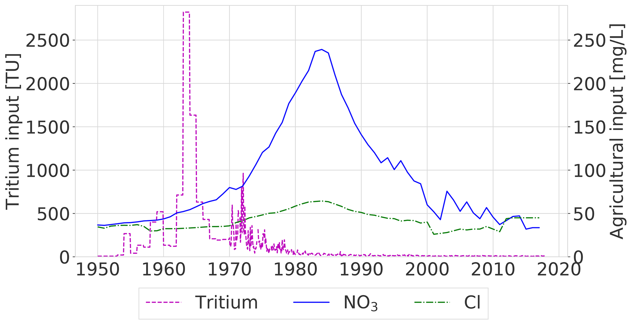
Figure 3Input time series for tritium (left axis) and the estimated concentrations of nitrate and chloride under farmland (right axis). The tritium input time series is based on precipitation measurements at stations in Vienna and Ottawa (before 1970) and Groningen and Emmerich (from 1970). The 1985 peak in chloride and nitrate coincides with the start of the legislations from the Dutch Manure Law that placed restrictions on the applications of N in agriculture.
3.2 Water quality measurements of surface water
Tritium concentrations measured in the upstream catchment in 2016 and 2017 were between 4.8 and 6.0 TU, with no clear seasonality (Fig. 4a). For chloride and nitrate, the measurements show some seasonality, with higher concentrations in winter than in summer. This variability seems larger for the total catchment than for the upstream part of the catchment (Fig. 4).
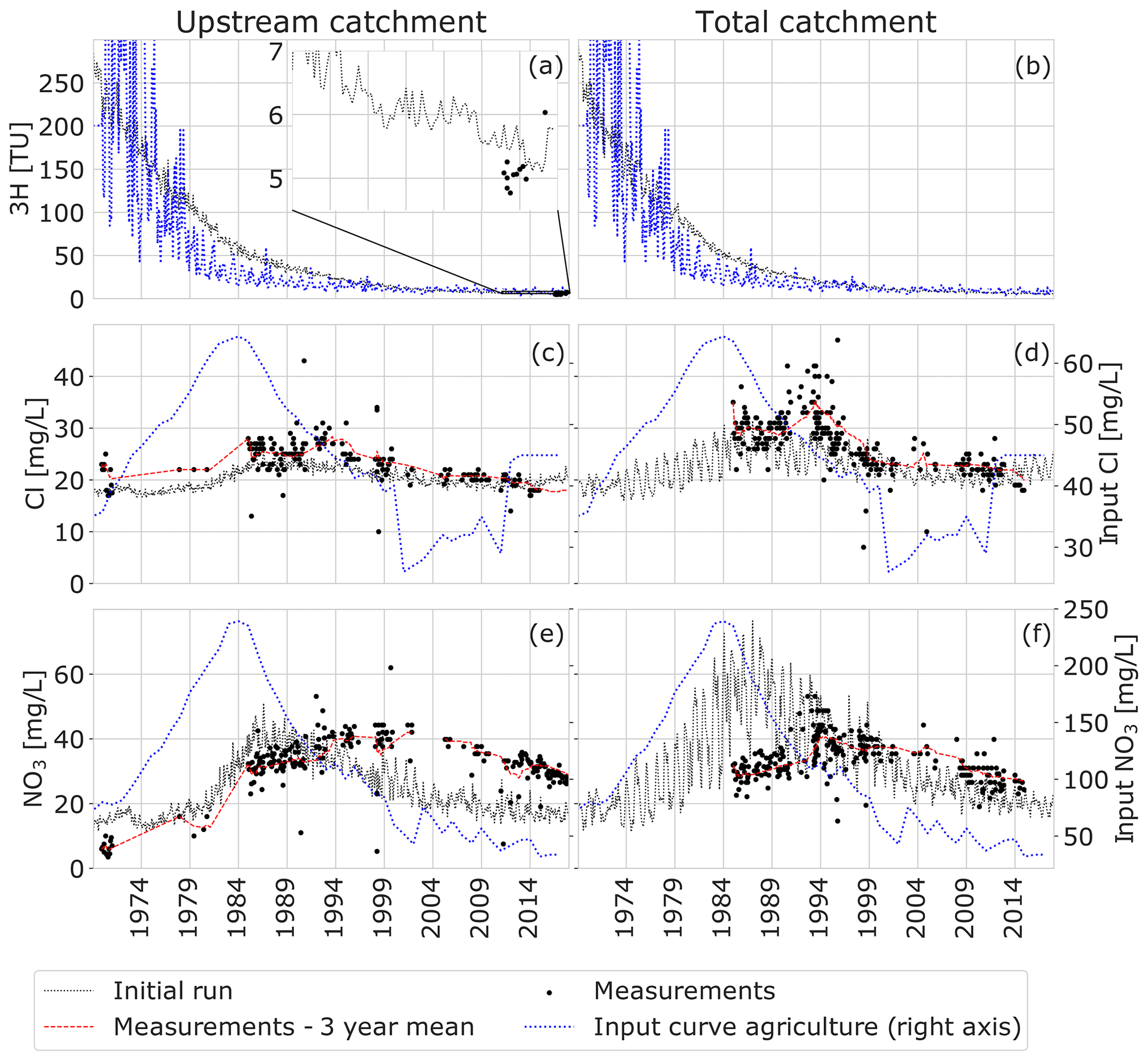
Figure 4Measurements, agricultural input time series, and initial model results based on the TTDs from Kaandorp et al. (2018a) and the solute input time series in Fig. 3. On the left, tritium (a), chloride (c), and nitrate (e) are shown for the upstream part of the catchment; on the right, tritium (b), chloride (d), and nitrate (f) are shown for the total catchment (downstream). Note that tritium samples were only available for the upstream part of the catchment (a).
The long-term chloride concentrations varied between 20 and 40 mg L−1, with slightly lower values in the upstream than in the downstream catchment. Nitrate concentrations varied between approximately 25 and 50 mg L−1 during the last few decades. Both the chloride and nitrate measurements show a clear trend reversal (Fig. 4c–f) that resembles the trend reversal in the solute input time series (Fig. 3) due to legislations. Chloride concentrations in the upstream part of the catchment increase from about 20 mg L−1 in the 1970s to up to 30 mg L−1 between 1990 and 1994 (Fig. 4c), which is a time lag of about 5 to 10 years after the peak in the input around 1985 (Fig. 3). Chloride concentrations measured at the outlet of the total catchment peak at the same moment at a concentration of about 42 mg L−1 (Fig. 4d). After 1994, the chloride concentrations decrease both up- and downstream and have been approximately stable between 20 and 25 mg L−1 since the year 2000, which is similar to the trend in the chloride concentrations in the uppermost groundwater (solute input time series). The measured timing of the trend reversal of nitrate at the outlet of the catchment (Fig. 4f) is similar to chloride (Fig. 4d), with an increase up to 1994 when the maximum of 50 mg L−1 is reached. After that, nitrate concentrations have decreased but at a slower rate than chloride. What is especially noticeable is that, for the upstream part of the catchment, the timing of the chloride and nitrate peaks in the measurements do not coincide. While chloride peaks between 1990 and 1994 and quickly drops after that, nitrate concentrations only start decreasing after approximately 1997. Thus, for the upstream catchment there seems to be a time lag between the peak input and the following trend reversal that is several years longer than observed in the downstream catchment.
3.3 Water quality modelling
The initial combination of the TTD results and solute input time series was based on the land use and input time series described in Sect. 2.5 and included no further processes or changes to the original flow model. The initial model run showed higher chloride and nitrate concentrations in winter than in summer, and this seasonal variation was larger for the total catchment than the upstream catchment. Such a difference between the up- and downstream part of the catchment was also found by Kaandorp et al. (2018a), who reported that discharge and the contribution of different flow paths are more dynamic in the downstream part of the catchment.
The modelled chloride concentrations confirmed the observed long-term trends (Fig. 4c and d), although the modelled concentrations were too low for the period between 1990 and 1995 (underestimation of 5–15 mg L−1), and the chloride peak was simulated around 1985 instead of 1990. For tritium, the model overestimates the measured concentrations by approximately 0.5 TU (Fig. 4a), which could indicate either an underestimation of the mean age of water in the catchment (allowing for more decay) or an underestimation of the amount of younger or pre-1950s water (contributing water with low tritium concentrations). While the measurements showed the nitrate peak around 1994 and 1997 for the total catchment and upstream respectively, the initial model run showed the nitrate peak around 1987 for both the total and upstream catchment. In this model calculation, the modelled trend reversal for nitrate thus occurs approximately 3 years after the trend reversal in the input, which is the same time lag as was modelled for chloride.
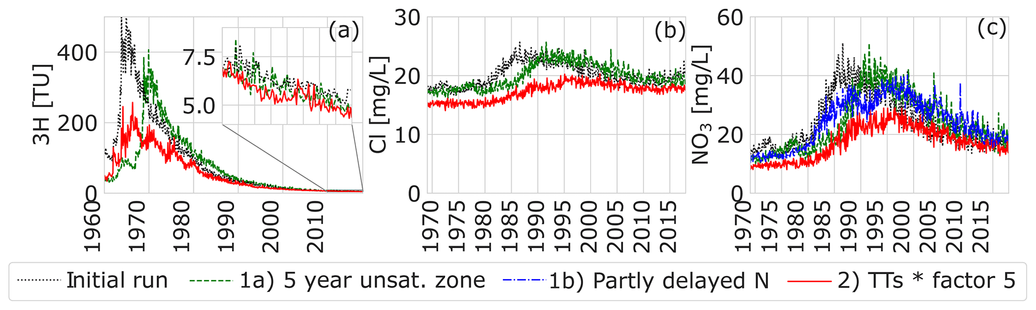
Figure 5The effect on tritium (a), chloride (b), and nitrate (c) in the upstream part of the catchment of a scenario with a 5-year delay due to an unsaturated zone, a scenario in which part of the input of N was delayed and a scenario in which all travel times were increased by a factor of 5.
Table 3Summarized results of the exploration of the model behaviour.
3.4 Exploration of model behaviour – effects on the breakthrough of tritium, chloride, and nitrate
Overall, the simulated tritium, chloride, and nitrate concentrations in the stream did not completely match the measurements either in concentration or in the arrival in time of the agricultural peak (Fig. 4). Instead of attempting to further adapt and calibrate the groundwater flow model, we explored the model behaviour under different scenarios, exploring the parameters that might determine the apparent mismatch with the measured concentrations, thereby increasing our understanding of the flow and transport system in catchments in general.
3.4.1 Set 1a – unsaturated zone hydrological delay
An unsaturated zone was added to the upstream catchment model, with a travel time of 5 years, as a separate piston flow component superimposed on the groundwater system that was modelled. This delay shifted the tritium peak in time and led to a decrease in the tritium concentrations because decay takes place while travelling through the unsaturated zone (Fig. 5a). This scenario lowered the modelled stream tritium concentrations closer to the observed tritium concentrations. Because chloride and nitrate were not reactive, this unsaturated zone scenario merely added a certain amount of time to the whole travel time distribution, simply shifting the chloride and nitrate output by 5 years (Table 3).
3.4.2 Set 1b – unsaturated zone N species delay
The time lag created in the unsaturated zone by the slower release of persistent N was simulated by putting a delay of 10 years on 50 % of the nitrate input. Because the input of nitrate is spread out over a longer period, this resulted in a peak value that was 11 mg L−1 lower but extended the duration of high nitrate levels (Table 3; Fig. 5c).
3.4.3 Set 2 – increased saturated zone travel times
The multiplication of the calculated mean travel times by a factor 5 decreased the overall tritium concentrations due to the extra time for decay (Fig. 5a). The input of solutes towards the stream was distributed more in time, which lowered the chloride and nitrate peak and increased the length and size of the tail of the peak (Fig. 5b and c). This scenario thus has a similar effect on the shape of the breakthrough of nitrate as scenario 1b (Fig. 5c). When all travel times were increased fivefold, the chloride and nitrate peaks shifted by approximately 10 years (Table 3).

Figure 6Panels (a) and (b) show the effect of two scenarios with changes in the nitrate input for the upstream of the catchment. Note the difference in the scale of the y axis between the left and right panels. Panels (c) and (d) show the effect of spatial changes in land use on both chloride (c) and nitrate (d), i.e. only agriculture inside of a 200 m strip around the stream (4a) and only agriculture outside of the same buffer strip (4b). In both scenarios, agricultural parts have 50 % agriculture and 50 % nature, so that the total fraction of fields is approximately equal to that in the real catchment.
3.4.4 Set 3 – different temporal input of solutes
We modelled two alternative solute input time series of agricultural fields. First, we removed all agricultural input after the 1985 nitrate peak (Fig. 6a; green line). This instantly lowered the stream nitrate concentrations from 1986 onwards, as the stream consists of a large amount of young water and, after the removal of agriculture, is only affected by nitrate from older flow paths that started before 1986 (Fig. 6b; green line). In scenario 3b, we used a solute input time series in which the rate of the decrease of nitrate after the 1985 peak is lowered (Fig. 6a; red line). This slower decrease in the agricultural input resulted in an increase of nitrate during a longer period, remarkably extending also into the period when the input is already decreasing and creating a time lag of 10 years to the trend reversal (Table 3), followed by a slower decrease after that (Fig. 6b; red line).
3.4.5 Set 4 – spatial differences in solute input
The effect of spatial changes of the input was modelled in two scenarios, i.e. one scenario where only the zone of 200 m around the stream was used for agriculture (4a), and one scenario where agricultural input only took place outside of the same 200 m zone (4b). With the agricultural fields directly around the stream (scenario 4a), the nitrate peak shifted back in time to 1985 (Fig. 6c), which is the year of maximum input (Fig. 3). With the agricultural fields in the more upstream parts of the catchment (scenario 4b), representing, for example, a natural buffer strip, the nitrate peak was delayed by 4 years and became flatter with a much slower decrease over time (Fig. 6d). This results from the fact that the fields further away are connected with the stream by longer flow paths with longer travel times. For the 200 m zone around the stream, the mean TT towards the stream is approximately 3 years, and for the area outside this zone, the mean TT is approximately 15 years (median TT 1 year vs. 12 years). When fields are further away, the agricultural input to the stream is distributed more over time, resulting in a lower peak but a longer tail with higher concentrations.
3.4.6 Set 5 – denitrification in the saturated zone
A total of two denitrification scenarios were modelled, using different conceptualizations. A zero-order denitrification, with a rate of 10 mg L−1 yr−1, resulted in continuously lower nitrate concentrations without a shift in time (Fig. 7). In scenario 5b, denitrification was modelled based on the depth that the particles flowed through for which nitrate was removed from all particles travelling through deeper layers (> model layer 2; >0.5–15 m below surface). This resulted in a rather steady decrease in nitrate concentrations in time, preserving the shape of the 1980s increase and subsequent decrease (Fig. 7).
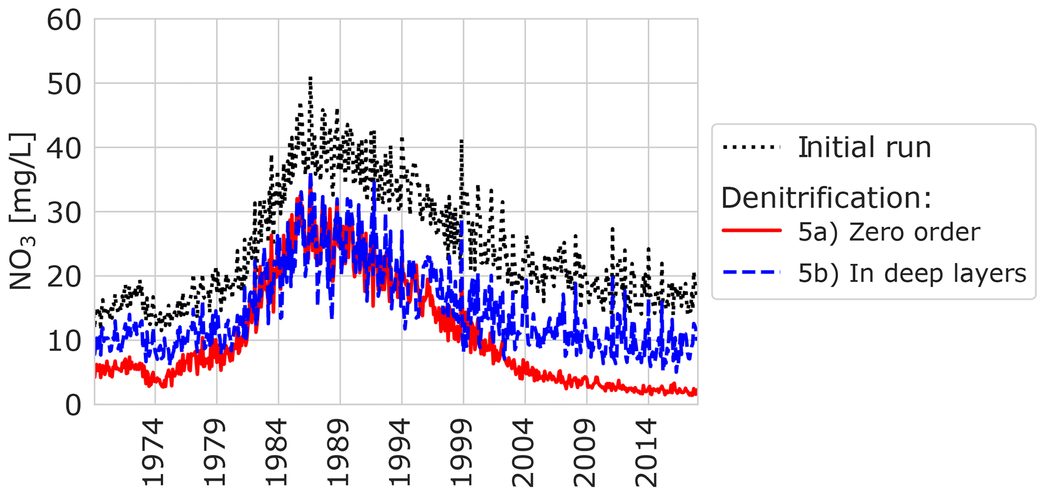
Figure 7Effect of denitrification for the upstream part of the catchment using different conceptualizations, i.e. zero-order denitrification (5a) and denitrification in deep layers (5b).
The aim of this study was to test whether the use of TTDs, as derived from a groundwater flow model, helps us to understand the observed breakthrough pattern of solutes in a lowland stream. We collected a long time series of chloride and nitrate, which showed a clear trend reversal in 1990, following national and European legislations restricting the use of manure and fertilizers. By combining the TTDs with input time series for solutes, we were able to calculate stream concentrations which we could compare with the long time series of chloride and nitrate. This base model, which did not include time delays due to the unsaturated zone or chemical processes, was able to reasonably capture the long-term trends of chloride and nitrate. However, this initial model run underestimated the time lag between the peak in nitrogen input and the following trend reversal of nitrate in the stream. In addition to the trend reversal in the 1990s, both the measurements and model indicated seasonality in the in-stream concentrations, with higher concentrations in winter and lower concentrations in summer (Sect. 3.2).
In the discussion, we will first focus on the effect of different processes on the breakthrough of solutes, based on the exploration of the model behaviour under different scenarios. We will evaluate how unsaturated zone processes, advective saturated flow, the spatial source zones and temporal patterns of solute inputs, and transformation processes such as denitrification will influence time lags in the receiving water body. Using our dynamic TTD model, we will then introduce contributing areas to discuss the spatial and temporal effects of land use and groundwater flow paths. We will subsequently discuss the measurements and model results of the study area and take another look at the observed breakthroughs and time lags of the different solutes. Lastly, we will discuss the implications of our findings for catchment management.
4.1 Changes in breakthrough patterns of tritium, chloride, and nitrate
The model exploration showed that unsaturated zones lead to a shift in time of the solute breakthrough, as it takes time for water to percolate from the surface towards the groundwater (Fig. 5; Table 3). This is purely a hydrological effect (scenario 1a). Biochemical processes in the unsaturated zone can also create time lags in the breakthrough of nitrate (scenario 1b). This not only lowers the height of the nitrate peak but also leads to a time lag and elevated nitrate levels over a longer period of time. The scenario in which the TTD of all flow paths was multiplied by a factor 5 lowered the peak of nitrate observed in the stream. The reason is that the mean age of the discharging groundwater was increased and resulted in a larger contribution of pre-1950 water, which has been less influenced by agricultural activities. In addition, the solutes applied by agriculture in the 1980s are distributed over a larger amount of time. In addition to lowering the peak, this resulted in a shift in the arrival of the trend reversal and a slower decrease in concentrations afterwards (Fig. 5; Table 3). The multiplication of the MTT has a clear effect on the breakthrough, but the factor 5 is a very extreme case. It would represent a system with an aquifer that is 5 times as thick (or with an unrealistic porosity 5 times higher) given the same groundwater recharge rate (van Ommen, 1986; Vogel, 1967).
Obviously, the solute input time series and its uncertainty have a large effect on the stream concentrations (Howden et al., 2011a). Changing the solute input time series led to a change in stream concentrations similar to that applied to the input. In scenario 3a, in which all agriculture was removed from the year 1986 onwards, nitrate concentrations in the stream instantly decreased. This follows from the relatively large amount of young water discharges by our catchment and is in line with the quick response observed for other catchments in the Netherlands (e.g. Rozemeijer et al., 2014). Van Ommen (1986) used a conceptual case to illustrate the same fast reaction; in catchments with an exponential TTD (or, in our case, close to exponential TTD; Kaandorp et al., 2018a), a change in the input directly affects stream concentrations for all MTTs. This is caused by the fact that the maximum of an exponential distribution is always at the beginning. In scenario 3b, the decrease of input concentrations after the trend reversal in the 1980s was more gradual. In this scenario, we did not shift the moment of the peak in the input because we have strong indications that the peak in Dutch agriculture occurred during the same year in all of the Netherlands due to the strict measures taken around 1985 (van den Brink et al., 2008; Visser et al., 2007). Surprisingly, a time lag occurred between peak input and the trend reversal, suggesting that a direct response to changes in the input is not always the case.
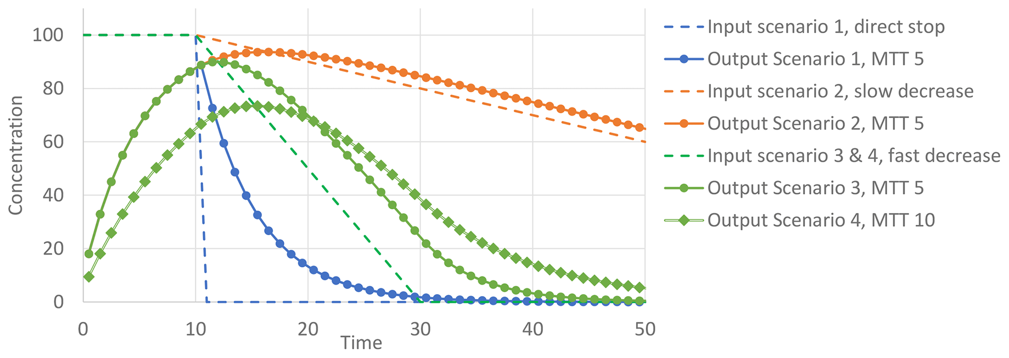
Figure 8Output concentrations for a hypothetical catchment with an exponential TTD and a MTT of 5 or 10, following three input scenarios, i.e. a direct stop of the input, a slow decrease in the input (decrease of 1 % in the maximum per time step), and a fast decrease in the input (decrease of 5 % in the maximum per time step).
To further study this observation, we did a conceptual exercise in which we combined exponential TTDs with varying MTTs with different conceptual input scenarios. Figure 8 illustrates three input scenarios for a conceptual catchment, with an exponential TTD, with a MTT of 5 or 10. The three input scenarios are a direct stop, a slow decrease of the input (decrease of 1 % of the maximum per time step), and a fast decrease of the input (decrease of 5 % of the maximum per time step), all following a block input of 100 between time equal to 0 and time equal to 10. A direct stop leads to a direct decrease in output concentrations, showing an inverse exponential distribution, which represents the new unpolluted front travelling through the groundwater system. The other three scenarios, on the contrary, do not show a direct decrease; the scenario with the fast decrease of the input and a MTT of 5 shows a concentration increase for 1 extra time step before decreasing, and this decrease is much slower than the scenario with the direct input stop. When the same input scenario is used with an MTT of 10, the time lag before the trend reversal is increased. The scenario with a slowly decreasing input shows the same, i.e. an increase in output concentration until t=16, even while the input decreases in that period. The time lag thus increases with increasing MTTs and with slower decreasing input. This behaviour is only the result of the hydrology of the groundwater system and is related to the net result of mass loading through groundwater recharge and mass removal at the outflow point. Concentrations at the outflow only start decreasing once the net input is smaller than the net output (Broers and van Geer, 2005). In other words, the output will only decrease when the nitrate input by recharge reaches a lower concentration than the convoluted output into the stream, as shown by the intersect of the input and output lines in Fig. 8. The time lag thus depends on the difference between the input and output concentrations. A longer MTT typically results in lower peak concentrations (see also scenario 2) and input concentrations will exceed those output concentrations for a longer time given the same reduction rate; it effectively takes longer for the input to decrease to the level of the output for a system with a longer MTT. This analysis shows that, in the general case of a catchment with an exponential groundwater TTD, the effect of measures on the solute input towards groundwater can only be expected to show directly when the decreased solute input is lower than the current concentration of the discharging water.
We saw that zero-order denitrification removes (part of) the nitrate and thus lowers concentrations and does not change the timing of the peak (Table 3), which was expected as the denitrification takes place equally along all flow paths. Moreover, denitrification at larger depths (scenario 5b) did not shift the peak in the receiving stream either (Fig. 7; Table 3). Older flow paths contribute a relatively steady amount of water and nitrate to the stream and removal of this contribution in this scenario led to a rather steady decrease in nitrate concentrations for all moments in time. Our scenarios were relatively simple, with equal denitrification rates and depths throughout the catchment. It is, however, known that there is a large variability in the reactivity of for instance organic matters (e.g. Hartog et al., 2004; Middelburg, 1989; Postma et al., 1991), which could lead to spatial or temporal differences in denitrification and, therefore, a change in the nitrate breakthrough. If denitrification, for instance, occurs predominantly in the stream valley close to the stream, where conditions are wet and organic matter is abundant, denitrification removes nitrate mostly from younger flow paths, thus shifting the nitrate peak due to the delivery of nitrate mostly by older flow paths, which generally originate from a larger distance from the stream (e.g. Modica et al., 1998). Such a spatial effect was also shown by the model scenario in which a buffer without agriculture was introduced around surface waters (Fig. 6c and d) and is a result of the difference in travel time of the flow paths from the fields close to the stream and the fields more upstream (e.g. Musolff et al., 2017).
The location of agricultural fields in relation to the catchments' drainage network and, more precisely, the location of high loading is, thus, another important factor that largely governs the travel times of the agricultural solutes. Both seasonal and long-term concentration–discharge relationships strongly depend on spatial source patterns (e.g. Musolff et al., 2017), and spatial differences in reactivity (e.g. Kolbe et al., 2019) can further cause spatial variability between solute concentrations of water in different flow paths. It can, therefore, be argued that, in modelling, not only the location of fields must be known but also more information about leaching towards the groundwater at every field, as there can be a significant difference in the use of manure and fertilizers due to, for instance, differences in crops. However, for our catchment, national and EU regulations put strong constraints on the application of nitrogen, thus levelling differences in inputs to farmlands (e.g. Oenema et al., 1998; Schroder et al., 2007). Effectively, soil properties and groundwater levels determine the areas with the strongest leaching towards the groundwater, as those factors determine the potential for unsaturated zone denitrification.
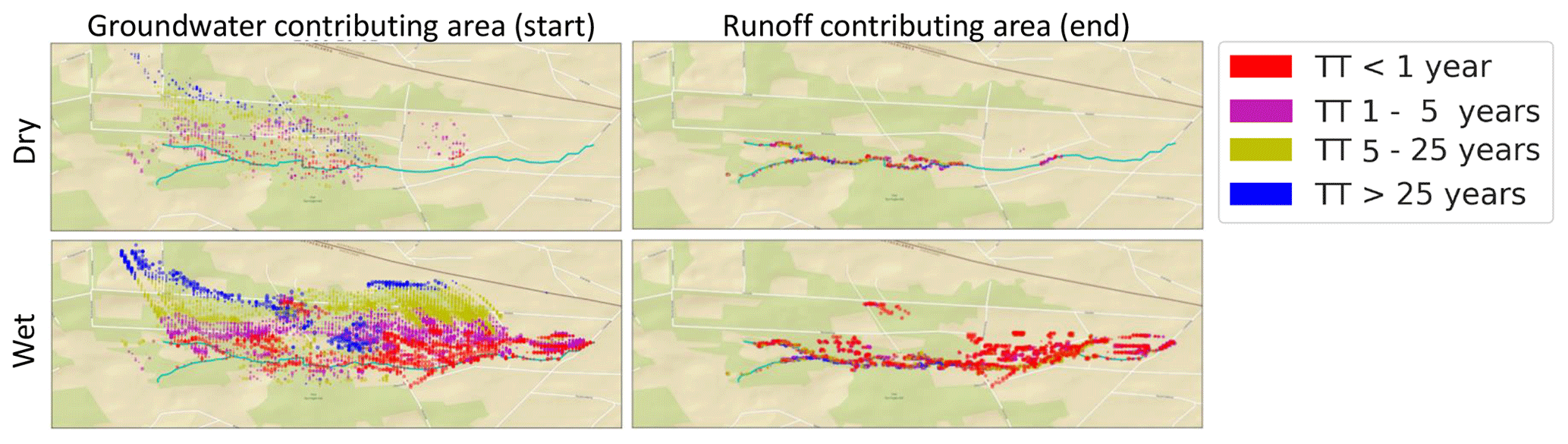
Figure 9Contributing area in the model for a dry (top; summer 2006) and a wet (bottom; winter 2006–2007) period. Colours represent the travel time towards the stream with blue TT > 25 year and red TT < 1 year (similar to Fig. 2). Notice the large increase in the runoff contributing area in the downstream part of the catchment during wet periods which results from the extensive agricultural drainage system. Background map source: ESRI_StreetMap_World_2D, available at: http://services.arcgisonline.com/ArcGIS/rest/services/ESRI_StreetMap_World_2D/MapServer (last access: 28 June 2020).
4.2 Contributing area of streams
In the previous paragraph, we have seen that the spatial distribution of inputs and processes is an important factor in the breakthrough of agricultural solutes. In our model, particles have a starting point and ending point for which we introduce the terms groundwater contributing area (GCA) and runoff contributing area (RCA; Fig. 9). The GCA is defined as the area in which the water that is actively contributing to streamflow at a certain moment in time through active flow paths entered the coupled groundwater–surface water system as precipitation. This is, thus, not the same as the catchment of a stream, which is the area in which all discharging water finally ends up in the stream, and does not include a time-variable component. The RCA is defined as the area in which, at a certain moment in time, water is leaving the subsurface domain (catchment storage) to become discharge and, thus, is the area where runoff is generated (Fig. 10). Within this catchment, areas that are neither groundwater nor runoff contributing areas do not actively contribute to streamflow at that specific moment in time. The concept of contributing areas can thus be used as a different way of describing the catchment and spatial processes and their effect on stream chemistry.
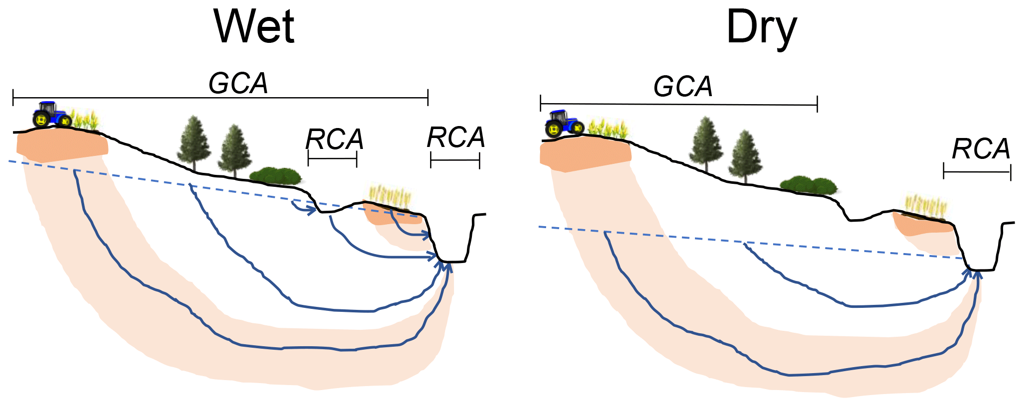
Figure 10Contributing areas fluctuate with wetness conditions due to changing flow paths. GCA is the groundwater contributing area, which is where discharge was infiltrated, and RCA is the runoff contributing area, which is where discharge is generated. Areas between the two different contributing areas are inactive and do not actively influence stream discharge.
Because flow paths change based on wetness conditions (e.g. Kaandorp et al., 2018a; Rozemeijer and Broers, 2007; Yang et al., 2018) the groundwater contributing area also shifts through the seasons. This includes the inactivation of flow through shallow flow paths towards, for example, drainage pipes and ditches in dry periods, which leads to a non-linear reaction of the dynamic TTD to discharge. When wetness conditions decrease, groundwater levels decrease and drainage units fall dry. Consequently, the water that was flowing towards these drainage units suddenly stays in the aquifer and/or flows towards another drainage unit. When wetness conditions increase again, groundwater levels first have to rise to the point that they can activate these flow paths again. This also (at least partly) explains why concentration–discharge relationships vary with the wetness of catchments. In our results, the discharge originating from agricultural fields changes in time as a result of this variation in the GCA (Figs. 2 and 9), and this seasonal variation in flow paths leads to fluctuations in the concentrations of nitrate in the stream (e.g. Fig. 4). Figure 10 illustrates how the groundwater contributing area may shift based on wetness conditions; in the wet period, all flow paths are active, while during the dry period only the older flow paths are active and flow through shallow short flow paths has ceased. Therefore, in this example, the groundwater contribution of the field close to the stream stops in the dry period, and removing this field, thus, only affects stream nitrate concentrations during the wet period. This concept extends on the ideas presented by Rozemeijer and Broers (2007) by adding the spatial dimension and groundwater contributing area to their concept of variation in the contribution of flow paths with depth. Information about the GCA is important for solute transport, as time lags occur if there is a difference between the forward TTD of the nitrate-contributing areas and the forward TTD of the entire catchment.
4.3 Understanding nitrate in the Springendalse Beek catchment
The previous paragraphs discussed the important processes that affect the breakthrough of agricultural solutes more generally, which we will use in this paragraph to discuss the observations from both the measurements and TTD model in the study area. Overall, the model was able to describe the trend reversal that was observed in the measurements of the Springendalse Beek catchment, but the time lag between the peak in nitrogen input and the following trend reversal of nitrate in the stream was underestimated. The time series of discharge and solutes showed that the upstream area has less seasonal variation in the amount of discharge than the downstream catchment and less variation in the contribution from agricultural fields and in the stream concentrations of chloride and nitrate (Figs. 3 and 4). Our groundwater-based model was able to simulate this difference between up- and downstream, which indicates that this variation can largely be explained by variations in the contribution of different groundwater flow paths originating from different locations in the catchment, as was also concluded by, for example, Martin et al. (2004), Musolff et al. (2016), Rozemeijer and Broers (2007), and van der Velde et al. (2010). High chloride and nitrate concentrations from agricultural activities are mostly present in the shallower layers (0–5 m below surface; e.g. Bohlke and Denver, 1995; Broers and van der Grift, 2004; Rozemeijer and Broers, 2007; van der Velde et al., 2009; Zhang et al., 2013) and especially in the downstream part of the catchment. The downstream catchment has a dense drainage network, with agricultural tile drains and ditches, which promotes a larger contribution of young water in shallow flow paths in the wet period with high groundwater tables relative to the dry period (Kaandorp et al., 2018a). This increase in relative old water contribution during dry periods has been found in several studies and is called the inverse storage effect (e.g. Benettin et al., 2017; Harman, 2015). Similar to our model, van der Velde et al. (2010) and Wriedt et al. (2007) were able to model seasonality of in-stream nitrate concentrations using only groundwater dynamics and concluded it to be an important process that is further superposed by denitrification and variability in loading. We conclude that the upstream part of the Springendalse Beek catchment, with its stable year-round discharge, provides a base level for nitrate concentrations, whereas the drained downstream part of the catchment causes the greater part of the seasonal variation in the stream concentrations.
The fact that most of the discharge has travel times larger than 1 year might explain that no seasonality was observed in the tritium measurements. The model overestimated all observed tritium concentrations in the initial model run by approximately 0.5 TU on average (Fig. 4a). This could indicate the uncertainty in the measured concentrations, but based on experience in other catchments (Broers and van Vliet, 2018a; Morgenstern et al., 2010; Stolp et al., 2010), this might be caused by the model underestimating the mean age of water in our catchment, for instance, due to an underestimation of the aquifer volume caused by the complex geology in the area. On the other hand, an overestimation of the mean water age by the model could also cause higher modelled tritium concentrations, if this means that the contribution of 1960s water is overestimated (Fig. 3). Unfortunately, no earlier measurements of tritium are available for the Springendalse Beek to draw further conclusions using tritium.
Denitrification does not seem to occur substantially in the upstream part of the study area, as the modelled nitrate concentrations are generally already lower than the measurements. This is confirmed by the oxic nature of the sandy sediments that the groundwater discharges from (Kaandorp et al., 2019), the presence of oxygen, and lack of iron in the discharge water (data not shown). Although the upstream part of the catchment contains less agriculture than the downstream part (Fig. 2), the nitrate concentrations in the stream are comparable. This may be an indication of denitrification in the downstream part of the catchment where water levels are close to the root zone, promoting shallow denitrification, which could be a reason for the overestimation of nitrate and the fact that the model overestimates the seasonal variation in the downstream catchment (Fig. 4f). Another important aspect is the uptake of nitrate and denitrification within the surface water system. This is currently not accounted for, and probably limited in winter (high flow velocities and low temperatures), but may be causing lower nitrate concentrations in summer.
Measurements of chloride and nitrate showed a time lag between the trend reversal in the solute input and in the discharge. In the lowland groundwater-driven study catchment, unsaturated zones are relatively thin in the downstream part of the catchment (a maximum of a few metres but mostly <1 m) and slightly thicker in the upstream part (up to 3 m), and thus, only a maximum time lag of a few years would be realistic. Due to the complex hydrogeology of the ice-pushed ridge, especially in the upstream part of the catchment, there is some uncertainty regarding the exact depths and volumes of the aquifers that are present within the ice-pushed ridge. In the regional groundwater flow model, this complex geology was highly simplified, based on the version of the hydrogeological model of the Netherlands, REGIS (REGIS II, 2005), that was available when building the flow model. The complex geological structure of the ice-pushed ridge makes it difficult to exactly pinpoint the position of the tilted Pleistocene sand layers that probably form the main pathways to the stream, as the tilted slabs of Tertiary clays form hydraulic barriers for groundwater flow (Ronald Harting, TNO Geological Survey of the Netherlands, personal communication, 2019). Given the approximate N–S strike direction of the sandy intercalations, this may have an influence on the distinct farmlands that contribute to the nitrate concentrations in the stream that may be positioned further away than the modelled schematization might allow in the regional groundwater flow model. It might also affect the mean travel times in the groundwater system, as a larger aquifer volume would result in overall longer travel times (Vogel, 1967; van Ommen, 1986). The observation that the time lag is larger for nitrate than for chloride, especially in the downstream catchment, can be explained by processes that only affect nitrate and not the more conservative chloride, such as a difference in residence time of different N species or spatial differences in denitrification. The difference could also indicate that the ratio between chloride and nitrate has changed in the fertilizers used.
Although a time lag was observed, the measurements showed that legislation in the 1980s and thereafter were effective at lowering the concentrations of agricultural solutes in the stream. The model was reasonably able to simulate the long-term trends but could be improved by adding more detail based on the lessons learnt from the model exploration. However, these lessons on the breakthrough of solutes are already applicable in other catchments and will be further discussed in the next paragraph.
4.4 Management implications
According to scenarios modelled by Tufford et al. (1998) the management of stream water quality is most effectively done at riparian and adjacent lands. Our results show that the location of agricultural fields indeed has a large effect on stream concentrations. Not only does the location of the fields affect the time lag and shape of the breakthrough of stream concentrations, longer flow paths from the fields further away from the stream also have more time for processes such as denitrification. Scenario 4b, with the 200 m agricultural-free zone around the stream, can be compared with a (natural) riparian zone on which much research has been done (e.g. Anderson et al., 2014; Feld et al., 2018; Hefting and Klein, 1998; Hill, 1996; Ranalli and Macalady, 2010). These studies show that riparian zones positively affect stream water quality because of their high rate of denitrification. Johnes and Heathwaite (1997) even suggested moving agricultural fields to the locations with the highest potential for nutrient retention. The importance of the spatial setting of land use in the landscape means that a map of forward TTDs combined with the locations of high solute input can be used for a vulnerability assessment of a catchment.
Our results further show that, in addition to the denitrification potential of a riparian buffer zone, the longer length of the groundwater flow paths lags the arrival of and dampens the nitrate peak. In fact, as denitrification rates are highly variable (e.g. Tesoriero and Puckett, 2011; Van Beek et al., 1994) and riparian zones can be by-passed by deeper groundwater flows (Bohlke and Denver, 1995; Flewelling et al., 2012; Hill, 1996; O'Toole et al., 2018; Ranalli and Macalady, 2010), the longer distance and, thus, the distribution of solutes in time may be the more important effect of riparian buffer zones. Therefore, creating a (significant) riparian buffer zone lags and dampens the effect of agricultural pollution on surface water quality and riparian buffers have a positive effect, even when it is bypassed or when denitrification is low. Although overall positively affecting water quality of the stream by decreasing concentrations, the longer travel times of agricultural solutes will also lead to a longer tail and, thus, invoke a longer-lasting effect of agricultural solutes on streams but at lower concentration levels.
The modelling approach, using travel time distributions, is a valuable approach for water quality management. While (ground)water models often focus on representing groundwater heads and discharges, a better representation of travel times and flow paths is essential to correctly simulate non-point source solute transport. Using TTDs therefore delivers more realistic scenarios for predicting future concentration trends and/or the effects of mitigation options.
This study is among the first to couple decades-long time series of water quality to dynamic travel time distributions based on a high-resolution spatially distributed groundwater flow model. We collected a unique data set of solute measurements for the period 1969–2018 for the Springendalse Beek, a Dutch lowland stream. We then combined calculated groundwater TTDs with input time series for tritium, chloride, and nitrate spanning the period 1950 to 2018. In this way, we calculated solute concentrations in the Springendalse Beek between 1969 and 2018. By making this connection between dynamic groundwater travel time distributions and long-term in-stream concentration measurements, we were able to show that the seasonal and long-term fluctuations of in-stream solute concentrations were mainly caused by the dynamic contribution of different groundwater flow paths.
Both the measurements and model showed a trend reversal in concentrations which followed the legislation to reduce the leaching of nitrate to groundwater in the 1980s. Because we observed a time lag of 5–10 years between the time of the peak in nitrate inputs to groundwater and the peak in nitrate concentrations in the stream, we ran an exploration of the model behaviour under different scenarios to explore the effect of different processes and parameters on the breakthrough patterns and time lags of groundwater-derived solutes. We found that a time lag towards the trend reversal of nitrate in the stream is caused by (1) longer travel times in the unsaturated zone, due to slow percolation, and retardation, due to (bio)chemical processes such as the slow mineralization of organic N, (2) the combination of a slow decrease in the nitrate input with a relatively long MTT, causing a prolonged period in which nitrate input concentrations still exceed the convoluted nitrate output discharging in the stream, and (3) spatial configurations of solutes input, locations of (bio)chemical processes, and drainage that promote older groundwater with higher nitrate loadings to dominate the outflow to the stream. This spatial effect may result from a higher input on older flow paths further from the drainage network (e.g. agricultural fields upstream) in combination with near-stream (bio)chemical attenuating processes in shorter flow paths (e.g. shallow denitrification in the riparian zone). To better describe the spatial effect of processes and land use on the breakthrough of solutes, we introduced the term groundwater contributing area, which is the catchment area where the discharging water infiltrated. This groundwater contributing area increases and shrinks based on wetness conditions, which leads to varying solute concentrations in the stream with wetness. Furthermore, we show that creating riparian buffer zones is a good management option, due to the importance of the spatial distribution and distance of agricultural fields and the reactivity of the subsurface on the breakthrough patterns of diffuse pollutants.
A limited amount of stream tritium measurements proved to be a valuable indication of the performance of the model. The method presented in this paper can be used to validate calculated TTDs and provides an opportunity to validate groundwater models not only on celerities but also on water velocities. Further research could be aimed at the application of the same method in other catchments and focus on gathering further knowledge on time lags and dynamic contributing areas in other hydrogeochemical and topographical settings.
Water quality model code and underlying and presented data can be found at https://doi.org/10.5281/zenodo.5039434 (Kaandorp, 2021).
The research was designed by VK, HPB, YvdV, and PdL. Field measurements and data collection were done by VK. Modelling was done by VK, HPB, and YvdV. All the authors participated in the analysis and discussion and helped prepare the article.
The authors declare that they have no conflict of interest.
We are grateful to the people of Water Board Vechtstromen and Rob van Dongen, from Staatsbosbeheer, for granting us access to water chemistry data, access to the field area, and the helpful discussions. We thank Bas van der Grift, for help with the agricultural input data.
This work is part of the MARS (Managing Aquatic ecosystems and water Resources under multiple Stress) project funded under the European Union's Seventh Framework Programme, Theme 6, Environment (including climate change; grant no. 603378; http://www.mars-project.eu, last access: 18 April 2021) and was partly funded through GeoERA HOVER under the “Establishing the European Geological Surveys Research Area to deliver a Geological Service for Europe (GeoERA)” project funded as part of the European Union's Horizon 2020 research and innovation programme (grant no. 731166).
This paper was edited by Markus Hrachowitz and reviewed by three anonymous referees.
Ali, G., Birkel, C., Tetzlaff, D., Soulsby, C., McDonnell, J. J., and Tarolli, P.: A comparison of wetness indices for the prediction of observed connected saturated areas under contrasting conditions, Earth Surf. Proc. Land., 39, 399–413, https://doi.org/10.1002/esp.3506, 2014.
Anderson, T. R., Groffman, P. M., Kaushal, S. S., and Walter, M. T.: Shallow Groundwater Denitrification in Riparian Zones of a Headwater Agricultural Landscape, J. Environ. Qual., 43, 732–744, https://doi.org/10.2134/jeq2013.07.0303, 2014.
Aquilina, L., Vergnaud-Ayraud, V., Labasque, T., Bour, O., Molénat, J., Ruiz, L., de Montety, V., De Ridder, J., Roques, C., and Longuevergne, L.: Nitrate dynamics in agricultural catchments deduced from groundwater dating and long-term nitrate monitoring in surface- and groundwaters, Sci. Total Environ., 435–436, 167–178, https://doi.org/10.1016/j.scitotenv.2012.06.028, 2012.
Benettin, P., Rinaldo, A., and Botter, G.: Tracking residence times in hydrological systems: Forward and backward formulations, Hydrol. Process., 29, 5203–5213, https://doi.org/10.1002/hyp.10513, 2015.
Benettin, P., Soulsby, C., Birkel, C., Tetzlaff, D., Botter, G., and Rinaldo, A.: Using SAS functions and high-resolution isotope data to unravel travel time distributions in headwater catchments, Water Resour. Res., 53, 1864–1878, https://doi.org/10.1002/2016WR020117, 2017.
Birkel, C., Soulsby, C., and Tetzlaff, D.: Conceptual modelling to assess how the interplay of hydrological connectivity, catchment storage and tracer dynamics controls nonstationary water age estimates, Hydrol. Process., 29, 2956–2969, https://doi.org/10.1002/hyp.10414, 2015.
Bohlke, J. K. and Denver, J. M.: Combined use of ground- water dating, chemical, and isotopic analyses to resolve the history and fate of nitrate contamination in two agricultural watersheds, atlantic coastal Plain, Maryland, Water Resour. Res., 31, 2319–2339, https://doi.org/10.1029/95WR01584, 1995.
Boumans, L. J. M., Fraters, D., and Van Drecht, G.: Nitrate leaching in agriculture to upper groundwater in the sandy regions of the Netherlands during the 1992–1995 period, Environ. Monit. Assess., 102, 225–241, https://doi.org/10.1007/s10661-005-6023-5, 2005.
Boumans, L. J. M., Fraters, D., and Drecht, G.: Mapping nitrate leaching to upper groundwater in the sandy regions of The Netherlands, using conceptual knowledge, Environ. Monit. Assess., 137, 243–249, https://doi.org/10.1007/s10661-007-9756-5, 2008.
Boumans, L. J. M., Wattel-Koekkoek, E. J. W., and van der Swaluw, E.: Veranderingen in regen- en grondwaterkwaliteit als gevolg van atmosferische emissiereducties, RIVM Rapport 680720005/2012, Rijksinstituut voor Volksgezondheid en Milieu, Bilthoven, 2013.
Broers, H. P.: The spatial distribution of groundwater age for different geohydrological situations in the Netherlands: implications for groundwater quality monitoring at the regional scale, J. Hydrol., 299, 84–106, https://doi.org/10.1016/j.jhydrol.2004.04.023, 2004.
Broers, H. P. and van der Grift, B.: Regional monitoring of temporal changes in groundwater quality, J. Hydrol., 296, 192–220, https://doi.org/10.1016/j.jhydrol.2004.03.022, 2004.
Broers, H. P. and van Geer, F. C.: Monitoring strategies at phreatic wellfields: a 3D travel time approach., Ground Water, 43, 850–862, https://doi.org/10.1111/j.1745-6584.2005.00043.x, 2005.
Broers, H. P. and van Vliet, M. E.: Age-dating springs and spring-streams in South-Limburg (Dateringsonderzoek bronnen en bronbeken Zuid-Limburg), TNO-rapport TNO 2018 R10421, TNO, Utrecht, p. 21, 2018.
Cartwright, I. and Morgenstern, U.: Transit times from rainfall to baseflow in headwater catchments estimated using tritium: The Ovens River, Australia, Hydrol. Earth Syst. Sci., 19, 3771–3785, https://doi.org/10.5194/hess-19-3771-2015, 2015.
De Lange, W. J., Prinsen, G. F., Hoogewoud, J. C., Veldhuizen, A. A., Verkaik, J., Oude Essink, G. H. P., van Walsum, P. E. V., Delsman, J. R., Hunink, J. C., Massop, H. T. L. L., and Kroon, T.: An operational, multi-scale, multi-model system for consensus-based, integrated water management and policy analysis: The Netherlands Hydrological Instrument, Environ. Model. Softw., 59, 98–108, https://doi.org/10.1016/j.envsoft.2014.05.009, 2014.
Duffy, C. J. and Lee, D.-H.: Base Flow Response From Nonpoint Source Contamination' Simulated Spatial Variability in Source, Structure, and Initial Condition, Water Resour. Res., 28, 905–914, 1992.
Duvert, C., Stewart, M. K., Cendón, D. I., and Raiber, M.: Time series of tritium, stable isotopes and chloride reveal short-term variations in groundwater contribution to a stream, Hydrol. Earth Syst. Sci., 20, 257–277, https://doi.org/10.5194/hess-20-257-2016, 2016.
EEA: European waters – Assessment of status and pressures 2018, Publications Office of the European Union, Luxembourg, ISBN 978-92-9213-947-6, ISSN 1977-8449, https://doi.org/10.2800/303664, 2018.
Ehrhardt, S., Kumar, R., Fleckenstein, J. H., Attinger, S., and Musolff, A.: Trajectories of nitrate input and output in three nested catchments along a land use gradient, Hydrol. Earth Syst. Sci., 23, 3503–3524, https://doi.org/10.5194/hess-23-3503-2019, 2019.
Engdahl, N. B., McCallum, J. L., and Massoudieh, A.: Transient age distributions in subsurface hydrologic systems, J. Hydrol., 542, 88–100, https://doi.org/10.1016/j.jhydrol.2016.04.066, 2016.
EU Nitrates Directive: EC, Directive of the Council of 12 December 1991, concerning the protection of waters against pollution caused by nitrates form agricultural sources, 91/676/ EEC, European Community, Brussels, 1991.
Feld, C. K., Fernandes, M. R., Ferreira, M. T., Hering, D., Ormerod, S. J., Venohr, M., and Gutiérrez-Cánovas, C.: Evaluating riparian solutions to multiple stressor problems in river ecosystems – A conceptual study, Water Res., 139, 381–394, https://doi.org/10.1016/j.watres.2018.04.014, 2018.
Flewelling, S. A., Herman, J. S., Hornberger, G. M., and Mills, A. L.: Travel time controls the magnitude of nitrate discharge in groundwater bypassing the riparian zone to a stream on Virginia's coastal plain, Hydrol. Process., 26, 1242–1253, https://doi.org/10.1002/hyp.8219, 2012.
Fraters, D., van Leeuwen, T., Boumans, L. J. M., and Reijs, J.: Use of long-term monitoring data to derive a relationship between nitrogen surplus and nitrate leaching for grassland and arable land on well-drained sandy soils in the Netherlands, Acta Agric. Scand. B, 65, 144–154, https://doi.org/10.1080/09064710.2014.956789, 2015.
Green, C. T., Liao, L., Nolan, B. T., Juckem, P. F., Shope, C. L., Tesoriero, A. J., and Jurgens, B. C.: Regional Variability of Nitrate Fluxes in the Unsaturated Zone and Groundwater, Wisconsin, USA, Water Resour. Res., 54, 301–322, https://doi.org/10.1002/2017WR022012, 2018.
Gustard, A., Bullock, A., and Dixon, J. M.: Low flow estimation in the United Kingdom, available at: http://nora.nerc.ac.uk/id/eprint/6050/ (last access: 17 May 2017), 1992.
Gusyev, M. A., Abrams, D., Toews, M. W., Morgenstern, U., and Stewart, M. K.: A comparison of particle-tracking and solute transport methods for simulation of tritium concentrations and groundwater transit times in river water, Hydrol. Earth Syst. Sci., 18, 3109–3119, https://doi.org/10.5194/hess-18-3109-2014, 2014.
Hansen, B., Thorling, L., Dalgaard, T., and Erlandsen, M.: Trend reversal of nitrate in Danish groundwater – A reflection of agricultural practices and nitrogen surpluses since 1950, Environ. Sci. Technol., 45, 228–234, https://doi.org/10.1021/es102334u, 2011.
Harbaugh, A. W.: MODFLOW-2005, The U.S. Geological Survey Modular Ground-Water Model — the Ground-Water Flow Process, US Geol. Surv. Tech. Methods 253, US Geological Survey Techniques and Methods 6-A16, US Geological Survey, Reston, Virginia, 2005.
Harman, C. J.: Time-variable transit time distributions and transport: Theory and application to storage-dependent transport of chloride in a watershed, Water Resour. Res., 51, 1–30, https://doi.org/10.1002/2014WR015707, 2015.
Hartog, N., van Bergen, P. F., de Leeuw, J. W., and Griffioen, J.: Reactivity of organic matter in aquifer sediments: Geological and geochemical controls, Geochim. Cosmochim. Ac., 68, 1281–1292, https://doi.org/10.1016/j.gca.2003.09.004, 2004.
Hefting, M. M. and de Klein, J. J. M.: Nitrogen removal in buffer strips along a lowlandstream in the Netherlands: a pilot study, Environ. Pollut., 102, 521–526, https://doi.org/10.1016/s0269-7491(98)80078-x, 1998.
Hendriks, D. M. D., Kuijper, M. J. M., and van Ek, R.: Groundwater impact on environmental flow needs of streams in sandy catchments in the Netherlands, Hydrolog. Sci. J., 59, 1–16, https://doi.org/10.1080/02626667.2014.892601, 2014.
Higler, L. W., Repko, F. F., and Sinkeldam, J. A.: Hydrobiologische waarnemingen in het Springendal, RIN-rapport 81/16, Rijksinstituut voor Natuurbeheerd, Leersum, 1981.
Hill, A. R.: Nitrate Removal in Stream Riparian Zones, J. Environ. Qual., 25, 743–755, 1996.
Hoek, D.: Nutriëntenbelasting in de bovenloop van de Springendalse beek: een onderzoek naar de waterkwaliteit van een Twentse bronbeek in bestuurskundig alsmede civieltechnisch perpectief, Universiteit Twente, Twente, avaiable at: http://library.wur.nl/WebQuery/hydrotheek/2196989 (last access: 15 October 2019), 1992.
Howden, N. J. K., Burt, T. P., Mathias, S. A., Worrall, F., and Whelan, M. J.: Modelling long-term diffuse nitrate pollution at the catchment-scale: Data, parameter and epistemic uncertainty, J. Hydrol., 403, 337–351, https://doi.org/10.1016/j.jhydrol.2011.04.012, 2011a.
Howden, N. J. K., Burt, T. P., Worrall, F., Mathias, S., and Whelan, M. J.: Nitrate pollution in intensively farmed regions: What are the prospects for sustaining high-quality groundwater?, Water Resour. Res., 47, W00L02, https://doi.org/10.1029/2011WR010843, 2011b.
Hrachowitz, M., Soulsby, C., Tetzlaff, D., Dawson, J. J. C., Dunn, S. M., and Malcolm, I. A.: Using long-term data sets to understand transit times in contrasting headwater catchments, J. Hydrol., 367, 237–248, 2009.
Hrachowitz, M., Benettin, P., Breukelen, B. M., Fovet, O., Howden, N. J. K., Ruiz, L., van der Velde, Y., and Wade, A. J.: Transit times – the link between hydrology and water quality at the catchment scale, WIREs Water, 3, 629–657, https://doi.org/10.1002/wat2.1155, 2016.
IAEA/WMO: Global Network of Isotopes in Precipitation, The GNIP Database, available at: http://www.iaea.org/water, last access: November 2018.
Johnes, P. J. and Heathwaite, A. L.: Modelling the Impact of Land Use Change on Water Quality in Agricultural Catchments, Hydrol. Process., 11, 269–286, 1997.
Kaandorp, V. P.: Data and scripts belonging to “Time lags of nitrate, chloride, and tritium in streams assessed by dynamic groundwater flow tracking in a lowland landscape”, Zenodo, https://doi.org/10.5281/zenodo.5039434, 2021.
Kaandorp, V. P., de Louw, P. G. B., van der Velde, Y., and Broers, H. P.: Transient Groundwater Travel Time Distributions and Age-Ranked Storage–Discharge Relationships of Three Lowland Catchments, Water Resour. Res., 54, 4519–4536, https://doi.org/10.1029/2017WR022461, 2018a.
Kaandorp, V. P., Molina-Navarro, E., Andersen, H. E., Bloomfield, J. P., Kuijper, M. J. M., and de Louw, P. G. B.: A conceptual model for the analysis of multi-stressors in linked groundwater–surface water systems, Sci. Total Environ., 627, 880–895, https://doi.org/10.1016/j.scitotenv.2018.01.259, 2018b.
Kaandorp, V. P., Doornenbal, P. J., Kooi, H., Broers, H. P., and de Louw, P. G. B.: Temperature buffering by groundwater in ecologically valuable lowland streams under current and future climate conditions, J. Hydrol., 3, 100031, https://doi.org/10.1016/j.hydroa.2019.100031, 2019.
Kolbe, T., De Dreuzy, J., Abbott, B. W., Aquilina, L., and Babey, T.: Stratification of reactivity determines nitrate removal in groundwater, P. Natl. Acad. Sci. USA, 116, 2494–2499, https://doi.org/10.1073/pnas.1816892116, 2019.
Kros, J., Tietema, A., Mol-Dijkstra, J. P., and de Vries, W.: Quantification of nitrate leaching from forest soils on a national scale in The Netherlands, Hydrol. Earth Syst. Sci., 8, 813–822, https://doi.org/10.5194/hess-8-813-2004, 2004.
Kuijper, M. J. M., Goorden, N., and Vermeulen, P. T. M.: Update Grondwatermodel Waterschap Regge en Dinkel, Deltares Report 1202490-000, Deltares, Utrecht, 2012.
Lutz, S. R., Trauth, N., Musolff, A., Van Breukelen, B. M., Knöller, K., and Fleckenstein, J. H.: How important is denitrification in riparian zones? Combining end-member mixing and isotope modeling to quantify nitrate removal from riparian groundwater, Water Resour. Res., 56, e2019WR025528, https://doi.org/10.1029/2019WR025528, 2020.
Martin, C., Aquilina, L., Gascuel-Odoux, C., Molénat, J., Faucheux, M., and Ruiz, L.: Seasonal and interannual variations of nitrate and chloride in stream waters related to spatial and temporal patterns of groundwater concentrations in agricultural catchments, Hydrol. Process., 18, 1237–1254, https://doi.org/10.1002/hyp.1395, 2004.
McDonnell, J. J., McGuire, K. J., Aggarwal, P., Beven, K. J., Biondi, D., Destouni, G., Dunn, S. M., James, a., Kirchner, J. W., Kraft, P., Lyon, S., Maloszewski, P., Newman, B., Pfister, L., Rinaldo, A., Rodhe, A., Sayama, T., Seibert, J., Solomon, D. K., Soulsby, C., Stewart, M. K., Tetzlaff, D., Tobin, C., Troch, P., Weiler, M., Western, A., Wörman, A., and Wrede, S.: How old is streamwater? Open questions in catchment transit time conceptualization, modelling and analysis, Hydrol. Process., 24, 1745–1754, https://doi.org/10.1002/hyp.7796, 2010.
McGuire, K. J. and McDonnell, J. J.: Hydrological connectivity of hillslopes and streams: Characteristic time scales and nonlinearities, Water Resour. Res., 46, W10543, https://doi.org/10.1029/2010WR009341, 2010.
Meinardi, C. R.: Groundwater recharge and travel times in the sandy regions of the Netherlands, Vrije Universiteit Amsterdam, available at: http://dare.ubvu.vu.nl//handle/1871/12739 (last access: 3 February 2019), 1994.
Middelburg, J. J.: A simple rate model for organic matter decomposition in marine sediments, Geochim. Cosmochim. Ac., 53, 1577–1581, 1989.
Modica, E., Buxton, H. T., and Plummer, L. N.: Evaluating the source and residence times of groundwater seepage to streams, New Jersey Coastal Plain, Water Resour. Res., 34, 2797–2810, 1998.
Morgenstern, U., Stewart, M. K., and Stenger, R.: Dating of streamwater using tritium in a post nuclear bomb pulse world: continuous variation of mean transit time with streamflow, Hydrol. Earth Syst. Sci., 14, 2289–2301, https://doi.org/10.5194/hess-14-2289-2010, 2010.
Musolff, A., Schmidt, C., Rode, M., Lischeid, G., Weise, S. M., and Fleckenstein, J. H.: Groundwater head controls nitrate export from an agricultural lowland catchment, Adv. Water Resour., 96, 95–107, https://doi.org/10.1016/j.advwatres.2016.07.003, 2016.
Musolff, A., Fleckenstein, J. H., Rao, P. S. C., and Jawitz, J. W.: Emergent archetype patterns of coupled hydrologic and biogeochemical responses in catchments, Geophys. Res. Lett., 44, 4143–4151, https://doi.org/10.1002/2017GL072630, 2017.
Nijboer, R. C., Wiggers, R., van den Hoek, T. H., and van Rhenen-Kersten, C. H.: Herstel van een brongebied in natuurreservaat het Springendal, Wageningen, Alterra, Wageningen, 2003.
Oenema, O., Boers, P. C. M., van Eerdt, M. M., Fraters, B., van der Meer, H. G., Roest, C. W. J., Schroder, J. J., and Willems, W. J.: Leaching of nitrate from agriculture to groundwater: the effect of policies and measures in the Netherlands, Environ. Pollut., 102, 471–478, 1998.
O'Toole, P., Chambers, J. M., and Bell, R. W.: Understanding the characteristics of riparian zones in low relief, sandy catchments that affect their nutrient removal potential, Agric. Ecosyst. Environ., 258, 182–196, https://doi.org/10.1016/j.agee.2018.02.020, 2018.
Pollock, D. W.: User's guide for MODPATH: A particle tracking post-processing package for MODFLOW, US Geological Survey, Reston, Virginia, https://doi.org/10.3133/ofr94464, 1994.
Postma, D., Boesen, C., Kristiansen, H., and Larsen, F.: Nitrate Reduction in an Unconfined Sandy Aquifer: Water Chemistry, Reduction Processes, and Geochemical Modeling, Water Resour. Res., 27, 2027–2045, 1991.
Prommer, H. and Stuyfzand, P. J.: Identification of temperature-dependent water quality changes during a deep well injection experiment in a pyritic aquifer, Environ. Sci. Technol., 39, 2200–2209, https://doi.org/10.1021/es0486768, 2005.
Raats, P. A. C.: Convective Transport of Solutes by Steady State Flows I. General Theory, Agr. Water Manage., 1, 201–218, 1978.
Ranalli, A. J. and Macalady, D. L.: The importance of the riparian zone and in-stream processes in nitrate attenuation in undisturbed and agricultural watersheds – A review of the scientific literature, J. Hydrol., 389, 406–415, https://doi.org/10.1016/j.jhydrol.2010.05.045, 2010.
REGIS II, Hydrogeological model of The Netherlands, Report: Vernes, R .W., Van Doorn, Th. H. M. From Guide layer to Hydrogeological Unit, Explanation of the construction of the data set, TNO report NITG 05–038-B, available at: https://www.dinoloket.nl/ (last access: 8 February 2019), 2005.
Rodriguez, N. B., Benettin, P., and Klaus, J.: Multimodal water age distributions and the challenge of complex hydrological landscapes, Hydrol. Process., 34, 2707–2724, https://doi.org/10.1002/hyp.13770, 2020.
Rozemeijer, J. C. and Broers, H. P.: The groundwater contribution to surface water contamination in a region with intensive agricultural land use (Noord-Brabant, The Netherlands), Environ. Pollut., 148, 695–706, https://doi.org/10.1016/j.envpol.2007.01.028, 2007.
Rozemeijer, J. C., Klein, J., Broers, H. P., van Tol-Leenders, T. P., and van der Grift, B.: Water quality status and trends in agriculture-dominated headwaters; a national monitoring network for assessing the effectiveness of national and European manure legislation in The Netherlands, Environ. Monit. Assess., 186, 8981–8995, https://doi.org/10.1007/s10661-014-4059-0, 2014.
Schroder, J. J., Aarts, H. F. M., Van Middelkoop, J. C., Schils, R. L. M., Velthof, G. L., Fraters, B., and Willems, W. J.: Permissible manure and fertilizer use in dairy farming systems on sandy soils in The Netherlands to comply with the Nitrates Directive target, Eur. J. Agron., 27, 102–114, https://doi.org/10.1016/j.eja.2007.02.008, 2007.
Solomon, D. K., Gilmore, T. E., Solder, J. E., Kimball, B., and Genereux, D. P.: Evaluating an unconfined aquifer by analysis of age-dating tracers in streamwater, Water Resour. Res., 51, 8883–8899, https://doi.org/10.1002/2014WR016259, 2015.
Sprenger, M., Seeger, S., Blume, T., and Weiler, M.: Travel times in the vadose zone: Variability in space and time, Water Resour. Res., 52, 1–20, https://doi.org/10.1002/2014WR015716, 2016.
Steenvoorden, J. H. A. M., Roest, C. W. J., and Boers, P. C. M.: Simulation of nutrient losses to groundwaters and surface waters in The Netherlands, in: Freshwater Contamination (Proceedings of Rabat Symposium S4, April–May 1997), No. 243, IAHS Publ., Wallingford, Oxfordshire, UK, 392 pp., 1997.
Stewart, M. K., Morgenstern, U., Gusyev, M. A., and Małoszewski, P.: Aggregation effects on tritium-based mean transit times and young water fractions in spatially heterogeneous catchments and groundwater systems, Hydrol. Earth Syst. Sci., 21, 4615–4627, https://doi.org/10.5194/hess-21-4615-2017, 2017.
Stolp, B. J., Solomon, D. K., Suckow, A., Vitvar, T., Rank, D., Aggarwal, P., and Han, L. F.: Age dating base flow at springs and gaining streams using helium-3 and tritium: Fischa–Dagnitz system, southern Vienna Basin, Austria, Water Resour. Res., 46, 1–13, https://doi.org/10.1029/2009WR008006, 2010.
Sültenfuß, J., Roether, W., and Rhein, M.: The Bremen mass spectrometric facility for the measurement of helium isotopes, neon, and tritium in water of helium isotopes, Isotop. Environ. Health Stud., 45, 83–95, https://doi.org/10.1080/10256010902871929, 2009.
Tesoriero, A. J. and Puckett, L. J.: O2 reduction and denitrification rates in shallow aquifers, Water Resour. Res., 47, 1–17, https://doi.org/10.1029/2011WR010471, 2011.
Tesoriero, A. J., Liebscher, H., and Cox, S. E.: Mechanism and rate of denitrification in an agricultural watershed: Electron and mass balance along groundwater flow paths, Water Resour. Res., 36, 1545–1559, 2000.
Tufford, D. L., McKellar, H. N., and Hussey, J. R.: In-Stream Nonpoint Source Nutrient Prediction with Land-Use Proximity and Seasonality, J. Environ. Qual., 27, 100–111, https://doi.org/10.2134/jeq1998.00472425002700010015x, 1998.
Van Beek, C. G. E. M., Laeven, M. P., and Vogelaar, A. J.: Modellering denitrificatie in grondwater onder invloed van organisch materiaal, H2O, 27, 180–184, 1994.
Van Dam, H., Mertens, A., and Janmaat, L. M.: De invloed van atmosferische depositie op diatomeeën en chemische samenstelling van het water in sprengen, beken en bronnen, Wageningen, 1993.
van den Brink, C., Jan, W., van der Grift, B., de Ruiter, P. C., and Griffioen, J.: Using a groundwater quality negotiation support system to change land-use management near a drinking-water abstraction in the Netherlands, J. Hydrol., 350, 339–356, https://doi.org/10.1016/j.jhydrol.2007.10.046, 2008.
van der Aa, N. G. F. M., Goes, B. J. M., de Louw, P. G. B., den Otter, C., Reckman, J. W. T. M., and Stuurman, R. J.: Ecohydrologische Systeemanalyse Springendalse Beek, Delft, TNO-rapport 99-168-B, NITG TNO, Delft, 1999.
van der Velde, Y., de Rooij, G. H., and Torfs, P. J. J. F.: Catchment-scale non-linear groundwater–surface water interactions in densely drained lowland catchments, Hydrol. Earth Syst. Sci., 13, 1867–1885, https://doi.org/10.5194/hess-13-1867-2009, 2009.
van der Velde, Y., de Rooij, G. H., Rozemeijer, J. C., van Geer, F. C., and Broers, H. P.: Nitrate response of a lowland catchment: On the relation between stream concentration and travel time distribution dynamics, Water Resour. Res., 46, W11534, https://doi.org/10.1029/2010WR009105, 2010.
van der Velde, Y., Torfs, P. J. J. F., van der Zee, S. E. A. T. M., and Uijlenhoet, R.: Quantifying catchment-scale mixing and its effect on time-varying travel time distributions, Water Resour. Res., 48, W06536, https://doi.org/10.1029/2011WR011310, 2012.
Van Meter, K. J. and Basu N. B.: Time lags in watershed-scale nutrient transport: An exploration of dominant controls, Environ. Res. Lett., 12, 084017, https://doi.org/10.1088/1748-9326/aa7bf4, 2017.
van Ommen, H. C.: Influence of diffuse sources of contamination on the quality of outflowing groundwater including non-equilibrium adsorption and decomposition, J. Hydrol., 88, 79–95, https://doi.org/10.1016/0022-1694(86)90198-8, 1986.
van Walsum, P. E. V. and Groenendijk, P.: Quasi Steady-State Simulation of the Unsaturated Zone in Groundwater Modeling of Lowland Regions, Vadose Zone J., 7, 769–781, https://doi.org/10.2136/vzj2007.0146, 2008.
van Walsum, P. E. V. and Veldhuizen, A. A.: Integration of models using shared state variables: Implementation in the regional hydrologic modelling system SIMGRO, J. Hydrol., 409, 363–370, https://doi.org/10.1016/j.jhydrol.2011.08.036, 2011.
Verdonschot, P. F. M. and Loeb, R.: Effecten van grondwatertoevoer op oppervlaktewaterkwaliteit: Een casestudie in twee natuurgebieden, Wageningen, Alterra-rapport 1752, Alterra, Wageningen, 2008.
Verdonschot, P. F. M., van den Hoek, T. H., and van den Hoorn, M. W.: De effecten van bodemverhoging op het beekecosysteem van de Springendalse beek, Wageningen, Alterra-rapport 1075, Alterra, Wageningen, 2002.
Visser, A., Broers, H. P., van der Grift, B., and Bierkens, M. F. P.: Demonstrating trend reversal of groundwater quality in relation to time of recharge determined by 3H/3He., Environ. Pollut., 148, 797–807, https://doi.org/10.1016/j.envpol.2007.01.027, 2007.
Visser, A., Heerdink, R., Broers, H. P., and Bierkens, M. F. P.: Travel time distributions derived from particle tracking in groundwater models containing weak sinks, Groundwater, 47, 237–245, 2009.
Vogel, J. C.: Investigation of groundwater flow with radiocarbon, IAEA – International Atomic Energy Agency, Vienna, 1967.
Wang, L., Stuart, M. E., Bloomfield, J. P., Butcher, A. S., Gooddy, D. C., Mckenzie, A. A., Lewis, M. A., and Williams, A. T.: Prediction of the arrival of peak nitrate concentrations at the water table at the regional scale in Great Britain, Hydrol. Process., 26, 226–239, https://doi.org/10.1002/hyp.8164, 2012.
Worrall, F., Howden, N. J. K., and Burt, T. P.: Time series analysis of the world's longest fluvial nitrate record: Evidence for changing states of catchment saturation, Hydrol. Process., 29, 434–444, https://doi.org/10.1002/hyp.10164, 2015.
Wriedt, G., Spindler, J., Neef, T., Meißner, R., and Rode, M.: Groundwater dynamics and channel activity as major controls of in-stream nitrate concentrations in a lowland catchment system?, J. Hydrol., 343, 154–168, https://doi.org/10.1016/j.jhydrol.2007.06.010, 2007.
Yang, J., Heidbüchel, I., Musolff, A., Reinstorf, F., and Fleckenstein, J. H.: Exploring the Dynamics of Transit Times and Subsurface Mixing in a Small Agricultural Catchment, Water Resour. Res., 54, 2317–2335, https://doi.org/10.1002/2017WR021896, 2018.
Zhang, Y. C., Slomp, C. P., Broers, H. P., Passier, H. F., and Cappellen, P. Van: Denitrification coupled to pyrite oxidation and changes in groundwater quality in a shallow sandy aquifer, Geochim. Cosmochim. Ac., 73, 6716–6726, https://doi.org/10.1016/j.gca.2009.08.026, 2009.
Zhang, Y. C., Prommer, H., Broers, H. P., Slomp, C. P., Greskowiak, J., van der Grift, B., and Van Cappellen, P.: Model-based integration and analysis of biogeochemical and isotopic dynamics in a nitrate-polluted pyritic aquifer, Environ. Sci. Technol., 47, 10415–10422, https://doi.org/10.1021/es4023909, 2013.