the Creative Commons Attribution 4.0 License.
the Creative Commons Attribution 4.0 License.
 | 30 Jun 2021
The value of water isotope data on improving process understanding in a glacierized catchment on the Tibetan Plateau
Lide Tian
Zhihua He
Lili Shao
This study integrated a water isotope module into the hydrological model THREW (Tsinghua Representative Elementary Watershed) which has been successfully used in high and cold regions. Signatures of oxygen stable isotope (18O) of different water inputs and stores were simulated coupling with the simulations of runoff generation. Isotope measurements of precipitation water samples and assumed constant isotope signature of ice meltwater were used to force the isotope module. Isotope signatures of water stores such as snowpack and subsurface water were updated by an assumed completely mixing procedure. Fractionation effects of snowmelt and evapotranspiration were modeled in a Rayleigh fractionation approach. The isotope-aided model was subsequently applied for the quantification of runoff components and estimations of mean water travel time (MTT) and mean residence time (MRT) in the glacierized watershed of Karuxung river on the Tibetan Plateau. Model parameters were calibrated by three variants with different combinations of streamflow, snow cover area and isotopic composition of stream water. Modeled MTT and MRT were validated by estimates of a tracer-based sine-wave method. Results indicate that (1) the proposed model performs well on simultaneously reproducing the observations of streamflow, snow cover area and isotopic composition of stream water, despite the fact that only precipitation water samples were available for tracer input; (2) isotope data facilitate more robust estimations on contributions of runoff components (CRCs) to streamflow in the melting season, as well as on MTT and MRT; (3) involving isotope data for the model calibration obviously reduces uncertainties in the quantification of CRCs and estimations of MTT and MRT, through better constraining the competitions among different runoff processes induced by meltwater and rainfall. Our results inform scientists on the high value of water isotope data for improving process understanding in a glacierized basin on the Tibetan Plateau.
- Article
(4830 KB) - Full-text XML
- BibTeX
- EndNote


Glacierized catchments in mountainous regions are generally headwater catchments, which are of great interest because of their complex runoff-generation processes and important role on supplying water sources for downstream regions (Immerzeel et al., 2010). Stable isotopes in water (δ2H and δ18O) are powerful tools for investigating the water cycle and hydrological processes (Gat, 1996; Bowen et al., 2019). Isotopic composition of water changes with multiple ecological and hydrological processes and is affected by several environmental factors (Zhao et al., 2012; Wang et al., 2013); thus, it is frequently used to track the storage and transportation of water. Isotopic compositions generally distinguish between different water bodies and phases (Xi, 2014) and thus is widely used to determine the relative dominance of water sources, especially in the glacierized catchments (Kong et al., 2019; He et al., 2020). Water isotope data consequently have the potential for improving the understanding of hydrological processes in glacierized catchments.
The Tibetan Plateau, as a high mountainous cryosphere, is the source of many major rivers in Asia including Yarlung Tsangpo-Brahmaputra river, Ganges, Indus river, and so on (Li et al., 2019). Scientific understanding of hydrological processes in this region is critical in predicting the responses of water resources and water hazards to climate changes (Lutz et al., 2014; Immerzeel et al., 2010; Miller et al., 2012). River runoff in these basins is prominently fed by multiple water sources including snowmelt, glacier melt and rainfall (Li et al., 2019). Coupling with the strong spatiotemporal variabilities of meteorological inputs, the complicated runoff-generation processes imply big challenges in understanding the hydrological behaviors in glacierized basins on the Tibetan Plateau.
It is, therefore, of critical importance to quantify contributions of runoff components (CRCs) to streamflow in glacierized regions. Estimating CRCs by hydrological models is one of the commonly adopted methods (Weiler et al., 2018), which is particularly subject to the following challenges. First, modeled CRCs rely heavily on the model conceptualizations of the mixing and propagations of different water sources in the basin. Model configurations and corresponding parameters representing the storage capacities of soil layers and groundwater aquifers obviously affect the relative proportions of surface and subsurface flow to streamflow (Nepal et al., 2014). CRCs modeled by different hydrological models are thus rarely comparable (Tian et al., 2020). For example, Nepal et al. (2015) and Siderius et al. (2013) compared CRCs estimated by different glacio-hydrological models in glacierized basins in the Himalayan region and demonstrated considerable variations in the modeled CRCs. They attributed the difference to the variations in the model conceptualizations. Second, strong compensatory effects of the simulated runoff induced by precipitation and ice meltwater which were typically not well constrained in the model resulted in large variations in the modeled CRCs. For instance, modeling results from Duethmann et al. (2015) and Finger et al. (2015) indicated that overestimated precipitation-triggered runoff in the model can be easily compensated by an underestimated ice melt runoff and vice versa, especially in high-altitude glacierized basins where precipitation input has large uncertainty.
Tracer data of water stable isotope have been widely used to label runoff components in the popular end-member mixing approach (e.g., Kong and Pang, 2012; He et al., 2020). Its value for improving modeled CRCs, however, has not been sufficiently investigated. Previous applications of tracer-aided hydrological models which integrated the simulation of water isotopic compositions of different runoff components into the rainfall/melting-runoff processes in snow-dominated basins have demonstrated high values of water isotope data on diagnostically improving model structure and recognizing the dominance of runoff processes on streamflow (Capell et al., 2012; Delavau et al., 2017; Son and Sivapalan, 2007; Birkel et al., 2011; Stadnyk and Holmes, 2020). An early test of the isotope-aided hydrological model in a glacierized basin in Tianshan, Central Asia, by He et al. (2019) indicated that additional use of isotope data helped to constrain the internal apportionments of runoff components in the model and improved the estimation of CRCs at an event scale. However, exploring the values of water isotope data for hydrological modeling in glacierized basins is still limited to the low availability of water tracer data from field water sampling due to the harsh environment, especially for glacierized basins on the Tibetan Plateau. As far as we know, a glacio-hydrological model coupled with the simulations of isotope signatures has not been developed and tested in the Tibetan Plateau yet.
Quantifying the time from entrance of water to its exits is fundamental to understanding flow pathways and the storage and mixing processes (McGuire and McDonnell, 2006). Characterizing water travel time distribution (TTD) and mean travel time (MTT) in addition to the traditional focus on streamflow response allows us to be closer to getting the right answers for the right reasons (Hrachowitz et al., 2013). Despite the fact that TTD and MTT serve as good tools to diagnose unsuitable model structures and parameterizations (McMillan et al., 2012), it has been rarely quantified in glacierized basins. Plenty of convenient tools have been developed based on lumped parameter models, but their practical applications in glacierized basins are restricted by the time invariant assumption and the weakness on considering the strong spatiotemporal variability of runoff processes (van Huijgevoort et al., 2016) as well as the seasonal water inputs from snowmelt and glacier melt. Fully physically based water particle tracking approaches coupling with hydrological processes are only limited to small basins due to the heavy computation cost (Remondi et al., 2018). Conceptual models that used additional tracer storage compartments along with the flow and transport processes have provided crucial information on the dynamics of flow pathways and storage, but they rely heavily on the prior definitions of function shape (e.g., travel time distribution (TTD) in van der Velde et al., 2015; StorAge Selection function (SAS) in Benettin and Bertuzzo, 2018; age-ranked storage–discharge relation in Harman, 2019). In contrast, tracer-aided hydrological models that integrated the storage and transportation of conservative water tracers into the runoff-generation processes have been demonstrated as successful in estimating TTD and water ages as well as their time variances within snowmelt influenced basins (e.g., Soulsby et al., 2015; Ala-aho et al., 2017). However, such hydrological models have not been applied in glacierized basins for estimations of TTD and MTT yet.
For process understanding in glacierized basins, glacio-hydrological models that additionally represented the snow processes and glacier evolution have been widely used (e.g, Immerzee et al., 2013; Lutz et al., 2014, 2016; Luo et al., 2018). The more complex integration of water sources from different flow pathways and units resulted in expanded parameter space of these hydrological models, which introduced large uncertainty in the model calibration (Finger et al., 2015). Equifinality is serious in these regions when calibrating hydrological model by streamflow solely, indicating that different parameters and runoff component proportions could perform similarly in discharge simulations (Beven and Freer, 2001; Chen et al., 2017), despite the general good performance for streamflow simulation. Therefore, multiple datasets including glacier observation and remotely sensed snow products have been frequently used in addition to streamflow measurements in vast glacio-hydrological simulations (e.g., Parajka and Blöschl, 2008; Konz and Seibert, 2010; Schaefli and Huss, 2011; Duethmann et al., 2014; Finger et al., 2015; He et al., 2018). However, both discharge and snow/glacier measurements provide insufficient constraints on distributions of flow pathways and the parameterizations of subsurface water storages (He et al., 2019). Although application in a glacierized basin in Central Asia by He et al. (2019) indicated high utility of isotope data on constraining the complex interactions of multiple runoff processes for the quantifications of CRCs, the values of water tracers such as stable isotopes on reducing uncertainties in the estimations of TTD and MTT in glacierized basins on the Tibetan Plateau have not been investigated.
In light of those backgrounds, this study integrated the simulation of oxygen isotope signatures into a hydrological model that has been proved effective to simulate the runoff processes on the Tibetan Plateau. The developed tracer-aided hydrological model was applied to the Karuxung river catchment (286 km2, 4550 to 7206 m a.s.l.) on the Tibetan Plateau. The objectives of this study are (1) to test the capability of the proposed tracer-aided model on simultaneously reproducing streamflow and isotope signatures of stream water in the study basin where only precipitation water samples are available for isotope input, (2) to evaluate the values of tracer-aided method on improving the estimation of CRCs and TTD/MTT in the study basin, and (3) to assess and interpret the differences between modeled TTD/MTT and estimates by a lumped parameter method.
2.1 Study area and data
This study focuses on the Karuxung catchment, which is located in the upper region of the Yarlung Tsangpo river basin, on the northern slope of the Himalayan mountains (Fig. 1). Digital elevation model (DEM) data in the study catchment with a spatial resolution of 30 m were downloaded from the Geospatial Data Cloud (http://www.gscloud.cn, Last access: 1 January 2019). The Karuxung river originates from the Lejin Jangsan Peak of the Karola Mountain at 7206 m above sea level (a.s.l.) and flows into Yamdrok Lake at 4550 m a.s.l. (Zhang et al., 2006). The catchment covers an area of 286 km2. The river discharge is significantly influenced by the headwater glaciers which cover an area of around 58 km2 (Mi et al., 2001). This catchment is dominated by a semiarid climate. The mean annual temperature and precipitation at Langkazi weather station were 3.4∘ and 379 mm, respectively. Due to the effect of the South Asian monsoon, more than 90 % of the annual precipitation falls between June and September. Precipitation occurs mostly in the form of snow from October to the following March at high elevations (Zhang et al., 2015).
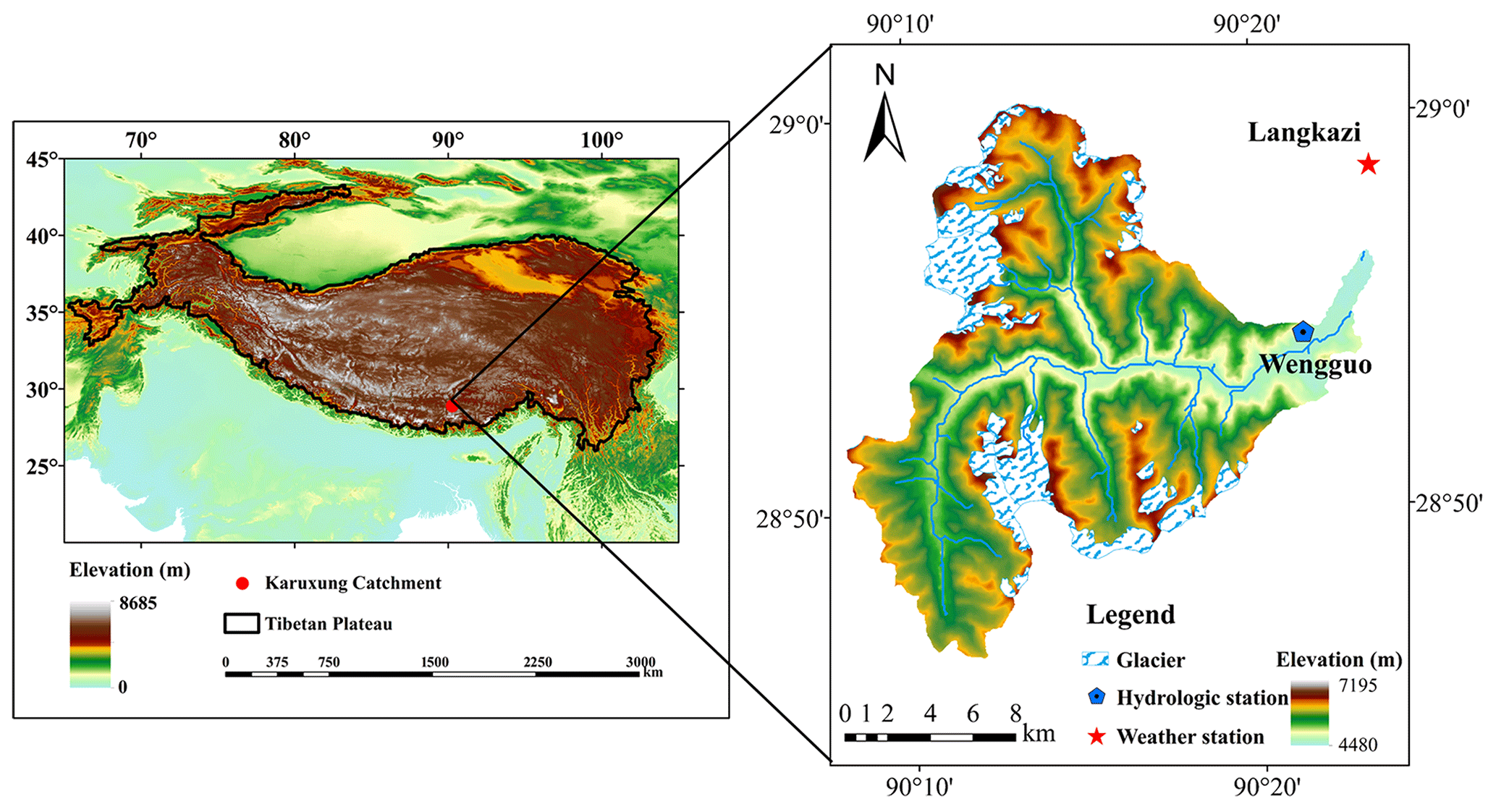
Figure 1Location and topography of the study area.
Daily temperature and precipitation data from 1 January 2006 to 30 September 2012 were collected at the Langkazi weather station (4432 m a.s.l.). Altitudinal distributions of temperature and precipitation across the catchment were estimated by the lapse rates reported in Zhang et al. (2015). Runoff data were measured daily from 1 April 2006 to 31 December 2012 at the Wengguo hydrological station at the catchment outlet. The coverages of glaciers were extracted from the Second Glacier Inventory Dataset of China (Liu, 2012). The 8 d snow cover extent data from MODIS product of MOD10A2 (500 m × 500 m; Hall and Riggs, 2016) were used to denote the fluctuations of the snow cover area (SCA). The 8 d leaf area index (LAI) and the monthly normalized difference vegetation index (NDVI) data were downloaded from MODIS product of MOD15A2H (500 m × 500 m; Myneni et al., 2015) and MOD13A3 (1 km × 1 km; Didan, 2015). Soil hydraulic parameters were estimated based on the soil properties extracted from the 1 km × 1 km Harmonized World Soil Database (HWSD, http://www.fao.org/geonetwork/, last access: 1 January 2019).
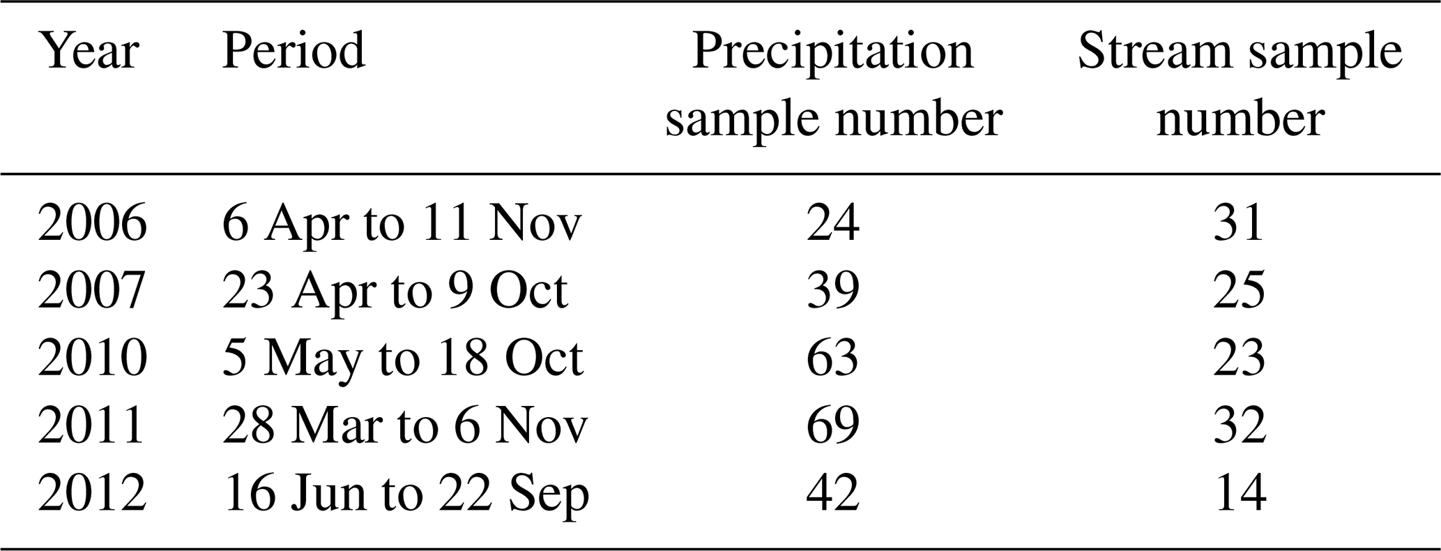
Grab samples of precipitation and stream water were collected at the Wengguo station in 2006–2007 and 2010–2012, for analysis of δ18O and δ2H, and the characteristics of samples are summarized in Table 1. In the dry seasons when precipitation water was not sampled due to small event amounts, precipitation isotope data from monthly Regionalized Cluster-based Water Isotope Prediction (RCWIP with a pixel size of 10′ × 10′; Terzer et al., 2013) were used as proxy for model input. The effect of elevation on the isotopic composition of precipitation was estimated using a lapse rate of −0.34 ‰ per 100 m based on Liu et al. (2007). The stream water samples were collected weekly every Monday from the river channel near the Wengguo station. Isotopic composition of glacier meltwater was assumed to be constant during the entire study period, and the value reported in Gao et al. (2009) was adopted.
2.2 Tracer-aided hydrological model
The THREW (Tsinghua Representative Elementary Watershed) model was originally developed by Tian et al. (2006), and it has been successfully applied to a wide range of catchments (e.g., Tian et al., 2012; Yang et al., 2014), including glacierized basins in the Alps, Tianshan, and the Tibetan Plateau (He et al., 2014, 2015; Xu et al., 2019). The THREW model uses the representative elementary watershed (REW) method for the spatial discretization of catchment, in which the study catchment is divided into REWs based on the catchment DEM, and then each of the REWs is divided into subzones as the basic units for hydrological simulation. More details of the model set up are given in Tian et al. (2006). In this study, the Karuxung catchment was divided into 41 REWs.
The snowmelt and glacier melt are differentiated according to the glacier coverage data. The meltwater in non-glacier areas is defined as snowmelt, and the meltwater in glacier-covered areas is defined as glacier melt, which includes the meltwater of both ice and snow. The two water sources are assumed to be melt at different rates, as represented by different degree-day factors. Meltwater from snow and glacier are simulated using a temperature-index method as given in Eqs. (1) and (2):
where the subscripts S and G represent snow and glacier, respectively. M is the melt amount, T is temperature and T0 refers to temperature threshold above which snow/ice starts to melt. DDF is the degree-day factor, representing the melt rate. Glacier meltwater (MG) in this study includes both ice melt and snowmelt on the glacierized area.
The fraction of snowfall (Ps) of the total precipitation P is determined by a temperature threshold Ts in Eq. (3). Snow water equivalent (SWE) of each REW is thus updated by Eq. (4). The snow cover area (SCA) of the corresponding REW is determined by a SWE threshold value (SWE0): when the calculated SWE is higher than SWE0, the SCA of this REW is recorded as 1; otherwise, the SCA is assumed to be 0 (similarly to Parajka and Blöschl, 2008; Zhang et al., 2015; He et al., 2014). The SCA of the whole study catchment is calculated as the ratio of the sum of the areas of snow-covered REWs to the total catchment area. Values of TN and SWE0 are set based on prior knowledge from Dou et al. (2011), Marques et al. (2011) and He et al. (2014): Ts=2 ∘C and SWE0= 20 mm.
Meltwater of ice and snow, as well as rainfall over the glacier area, are assumed to flow directly into the channel near the glacier tongue in the form of surface runoff, based on the low permeability of the glacier surface. Snowmelt in the non-glacier area is assumed to generate runoff in a similar way to rainfall (Schaefli et al., 2005). For model simplicity, the evolution of the glacier area is not simulated in the model for the short simulation period of 7 years.
Simulation of δ18O of multiple water sources was integrated into the runoff-generation processes in the THREW model (hereafter abbreviated as a THREW-t model). The δ18O of water sources in each of the subzones was assumed to be conservative, meaning that no chemical reactions occurred during the mixing of water sources. We assumed that the isotopic compositions of precipitation and glacier meltwater are linearly dependent on elevation, and we used linear gradients reported in Liu et al. (2007) to estimate the initial isotopic compositions of precipitation and glacier meltwater in individual REWs (similarly to He et al., 2019). The isotopic compositions of the snowpack and subsurface water storages were initialized by a “spin-up” running time for three hydrological years, assuming the isotopic compositions of water storages would reach steady levels after running for 3 years. Isotope composition of event snowfall on the snowpack was assumed to be the same as that of precipitation occurring in the corresponding REW.
The fractionation effects of evaporation on isotope composition of water were estimated by a Rayleigh fractionation method in Eqs. (5) to (7) (Hindshaw et al., 2011; Wolfe et al., 2007; He et al., 2019):
where is the isotope composition of the evaporated water, δ18Ox is the isotope composition of water before evaporation, α is the Rayleigh fractionation factor, T(K) is air temperature in the corresponding catchment unit, CF is a correction factor and f is the ratio of remaining water volume to the original water volume before evaporation.
A complete mixing assumption was used for the tracer signatures in each water storage. Consequently, δ18O of soil water and groundwater were updated according to the following equation:
where wo and δ18Oo are the water quantity and isotopic composition of the subsurface storages at the prior step, respectively. wi refers to the infiltration into the soil storage from water source i. For groundwater storage, wi refers to the seepage from upper soil water. δ18Oi stands for the isotopic composition of input water source i. The isotope signature of snowpack was simulated similarly as subsurface water storages according to Eq. (8).
Stream water in each of the REWs was considered a mixture of three components including inflow from the upstream REWs, runoff generated in the current REW and the water storage in the river channel. Consequently, the isotopic composition of stream water in each REW (δ18Or) was estimated based on the following conservative mixing equation:
where δ18Or0 is the isotopic composition of stream water, and wr is the water storage in the river channel at the time step before the mixing of runoff components. is the isotopic composition of stream water coming from the upstream REW k, and Ik is the inflow from the corresponding upstream REW. Subscripts of sur and gw refer to the surface runoff and subsurface flow from groundwater outflow generated in the current REW, respectively.
2.3 Model calibration
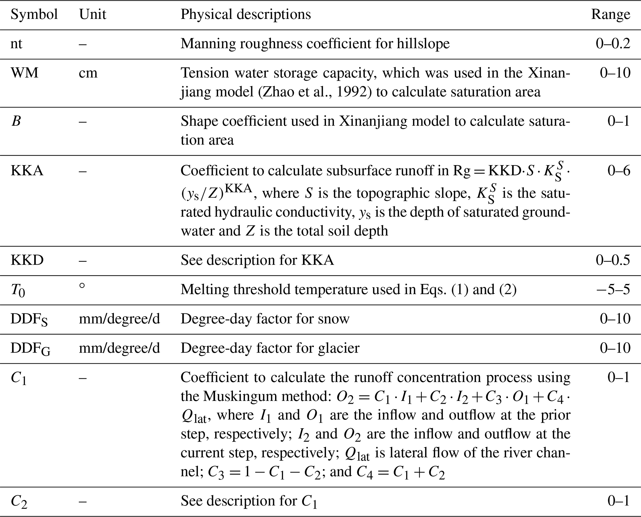
The physical meaning and value ranges of the calibrated parameters in the THREW-t model are described in Table 2. Parameter values were optimized using three calibration variants: (1) single-objective calibration using only the observed discharge at the catchment outlet, (2) dual-objective calibration using both observed discharge and MODIS SCA estimates, and (3) triple-objective calibration using observed discharge, MODIS SCA estimates, and δ18O measurements of stream water. Considering the data availability, we chose 1 April 2006 to 31 December 2010 as the calibration period and 1 January 2011 to 30 September 2012 as the validation period. For SCA, we used only the MODIS SCA estimates during the ablation period (1 May to 30 July) of each year for the model calibration, because simulations of runoff processes are mostly sensitive to the dynamics of snow cover extent in the melting period (Duethmann et al., 2014). Only the δ18O measurements of stream water in the rainy season (from the first rainfall event to the last rainfall event of each year, as shown in Table 1) were used to optimize the model parameters, because the measured isotope data for precipitation were only available in this season. We chose the objective functions of Nash–Sutcliffe efficiency coefficient (NSE) (Nash and Sutcliffe, 1970) and mean absolute error (MAE) to optimize the simulations of discharge, SCA and isotope, respectively (Eqs. 12–14).
where n is the total number of observations. Subscripts of o and s refer to observed and simulated variables, respectively. is the average value of observed streamflow during the assessing period.
An automatic procedure based on the pySOT optimization algorithm developed by Eriksson et al. (2017) was implemented for all the three calibration variants to identify the behavioral parameters. The pySOT algorithm used surrogate model to guide the search for improved solutions, with the advantage of requiring few function evaluations to find a good solution. An event-driven framework POAP (Plumbing for Optimization with Asynchronous Parallelism) was used for building and combining asynchronous optimization strategies. The optimization was stopped if a maximum number of allowed function evaluations was reached, which was set as 3000 in this study. For the single-, dual- and triple-objective calibration variants, NSEdis, NSEdis − MAESCA and NSEdis − MAESCA − MAEiso were chosen as combined optimization objectives, respectively. The pySOT algorithm was repeated 150 times for each calibration variant. The 150 final results were further filtered according to the metric of NSEdis; i.e., only the parameters producing NSEdis higher than a threshold were regarded as behavioral parameter sets. For single- and dual-objective calibration, the threshold was selected as 0.75. Considering the trade-off between discharge and isotope simulation, the threshold was chosen as 0.70 for triple-objective calibration. For each calibration variant, the parameter producing highest combined optimization objective was regarded as the best parameter set.
2.4 Quantifications of the contributions of runoff components to streamflow
The contributions of individual runoff components to streamflow were quantified based on two definitions of the runoff components. In the first definition, we quantified the contributions of individual water sources including rainfall, snow meltwater and glacier meltwater to the total water input, which were commonly reported in previous quantifications of runoff components on the Tibetan Plateau (Chen et al., 2017; Zhang et al., 2013). To be noted is that the sum of the three water sources should be larger than the simulated volume of runoff because of the evaporation loss. Thus, contributions quantified in this definition only refer to the fractions of the water sources in the total water input forcing runoff processes rather than the actual contributions of water sources to streamflow at the basin outlet. In the second definition, runoff components were quantified based on the runoff-generation processes including surface runoff and subsurface flow. Surface runoff consists of runoff triggered by rainfall and meltwater that feed streamflow through surface paths, as well as the precipitation occurring in river channel, and contributes to runoff directly. Subsurface flow is the interflow from groundwater outflow.
2.5 Estimation of the water travel time and residence time
In this study, the water travel time is estimated by the three methods, a lumped analytical method and two distributed model-based methods. A simplified lumped method, sine-wave method (SW) was used to provide a reference value of mean travel time (MTT) and mean residence time (MRT) in the catchment. The adopted model-based methods were developed by van Huijgevoort et al. (2016) and Remondi et al. (2018), which were referred to as mass-mixing method (MM) and flux-tracking method (FT), respectively. The SW method is based on the isotope data of precipitation and stream water. The MM and FT methods were conducted by the tracer-aided hydrological model using behavior parameter values identified by the calibration scenarios.
SW method has a stationarity assumption that a constant flow field gives constant travel time distributions (TTDs) (van der Velde et al., 2015). It assumes the form of TTD and derives the MTT directly from the series isotopic data (McGuire and McDonnell, 2006). Although the assumption is rather stringent, SW is widely used in the studies when an approximate estimation of MTT is required (e.g., Kirchner, 2016; Garvelmann et al., 2017). Here we assumed the form of TTD as the exponential function, and the MTT can be estimated according to Eqs. (13)–(14) (McGuire and McDonnell, 2006; Garvelmann et al., 2017):
where δt is the calculated δ18O of stream water or precipitation on day t of the year. is the mean δ18O of stream water or precipitation measured in different seasons. A and φ are parameters controlling the amplitude and phase lag, respectively, and are estimated based on the fitness between the sine-wave curve and the δ18O measurements. Subscripts of r and p in Eq. (14) represent river and precipitation, respectively.
The MM method was used to estimate the water age of outflow and water storage in the catchment. For the outflow (e.g., stream water, evaporation), the concept of water age is consistent with the concept of “travel time conditional on exit time” by Botter et al. (2011), “flux age” by Hrachowitz et al. (2013) and “backward travel time” by Harman and Kim (2014). For the water storage (e.g., soil water, groundwater, snowpack), the concept of water age is consistent with the concept of “residence time” by Botter at al. (2011) and “residence age” by Hrachowitz et al. (2013). The MM method regarded the water age as a kind of tracer and simulated the concentration of this tracer of the water bodies including snowpack, soil water and stream water (van Huijgevoort et al., 2016; Ala-aho et al., 2017). The “mass” and “concentration” of the water age were simulated similarly in Eqs. (8)–(9) by replacing δ18O with water age of the multiple terms. Event precipitation entering the catchment was treated as new water with a youngest age equal to the simulation step of the model. The glacier meltwater was regarded as very old water, and a constant age of 1000 d was adapted in this study. Meanwhile, the ages of water stored in snowpack, soil and river channel were assumed to increase with the ongoing simulation time: water age increased by 1 d after each model running at a daily step.
The FT method ran the model multiple times in parallel to track the fate of each precipitation event separately (Remondi et al., 2018). All days with precipitation were individually labeled and tracked over the simulation period by adding an artificial tracer to the water amounts which was assumed to not otherwise exist anywhere. The snow meltwater was tracked from the time when the snow entered the catchment as solid precipitation (i.e., snowfall) rather than the time when the snowpack melted. Glacier meltwater was not tracked, because the evolution of glacier was not simulated in the model, and the travel time of glacier melt as surface runoff was negligible. Similar to the MM method, the MTT of glacier melt runoff was assumed as a constant value as 1000 d. The mixing and transport processes of the tracer were also simulated similarly in Eqs. (8)–(9) by replacing δ18O with the concentration of the artificial tracer. By summarizing the mass of labeled precipitation in the water storage and stream water, the TTD conditional on exit time (backward TTD), TTD conditional on injection time (forward TTD) and residence time distribution (RTD) can be derived.
In summary, this study estimated the water travel time and residence time using a lumped method (SW) and two model-based methods (MM and FT), and the results of the three methods were compared to test the robustness of travel time estimation in this glacierized basin. Specifically, SW method estimated the MTT of total discharge and the MRT of water storage directly based on the isotopic data in stream water and precipitation. The MM method estimated the water age of stream water and groundwater storage, representing the daily backward MTT and MRT, respectively, and all 19 behavioral parameter sets of triple-objective calibration were used to illustrate the uncertainty of MTT. The FT method estimated the time-varying precipitation-triggered TTD and RTD, only using the parameter set producing best metric. To make the result of the FT method comparable to the MM method, the glacier melt runoff was also assumed to have MTT (water age) of 1000 d to calculate the MTT of the total runoff generation as the weighted average value of the MTT of precipitation runoff (including rainfall and snowmelt) and glacier melt runoff according to the contribution of water sources. The glacier melt was assumed to only contribute to surface runoff directly and exit the catchment rapidly and thus had no influence on the MRT estimation.
3.1 Model performance on the simulations of discharge and isotopic composition
For the calibration period, the single-objective calibration produced good performance for the simulation of discharge but had an extremely poor performance for the simulations of SCA and δ18O (Table 3). Involving SCA in the calibration objective, the dual-objective calibration significantly improved the simulation of SCA and kept a good behavior on discharge simulation but brought no benefit to the isotope simulation. The triple-objective variant led to a good performance for all the three metrics. The NSEdis produced by triple-objective calibration was slightly lower than that of the other two variants because of the lower threshold for behavior parameter sets. The simulation of isotopic composition of stream water was significantly improved by triple-objective calibration compared to the other two variants. For the validation period, the NSEdis of triple-objective calibration was significantly improved, even better than the single-objective, indicating the improved process representation of the behavior parameters by the triple-objective calibration. Through 150 runs of calibration program, the triple-objective calibration got the smallest behavior parameter sets, indicating that involving additional calibration objectives increases the identifiability of model parameters and reduces the equifinality.
Table 3Comparisons of the model performance produced by three calibration variants.
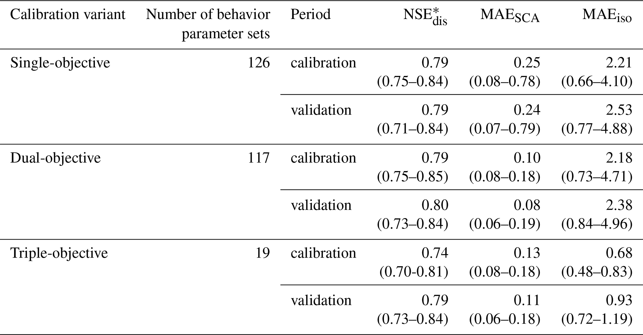
* Bracketed values represent the minimal and maximal values produced by the behavioral parameter sets.
Figure 2 shows the uncertainty ranges of the simulations for the behavioral parameters obtained by the three calibration variants. The three variants generally produced similar hydrographs in terms of the magnitudes and timing of peak flows with averaged behavioral parameter sets, but the triple-objective calibration had a narrower uncertainty range, especially for the baseflow-dominated periods (Fig. 2a–c). The single-objective variant resulted in rather large uncertainty ranges for the simulations of SCA and isotopic composition (Fig. 2d and g). The good fitness between the simulated and observed streamflow in summer is likely due to the largely overestimated rainfall-triggered surface runoff because of the underestimated reduction of SCA in spring. The dual-objective calibration significantly reduced the uncertainty range of the SCA simulation and captured the declining SCA in summer very well (Fig. 2e). Including SCA in the model calibration, however, only provided small benefits for the simulation of δ18O in stream water (Fig. 2h). Simulations of the triple-objective variant properly reproduced the temporal variation in SCA in the melt season, despite the slightly reduced performance compared to that of the dual-objective variant (behaving as higher MAESCA of triple-objective calibration in Table 3). Meanwhile, the seasonal variations of δ18O of stream water were reproduced well by the triple-objective calibration (Fig. 2i).
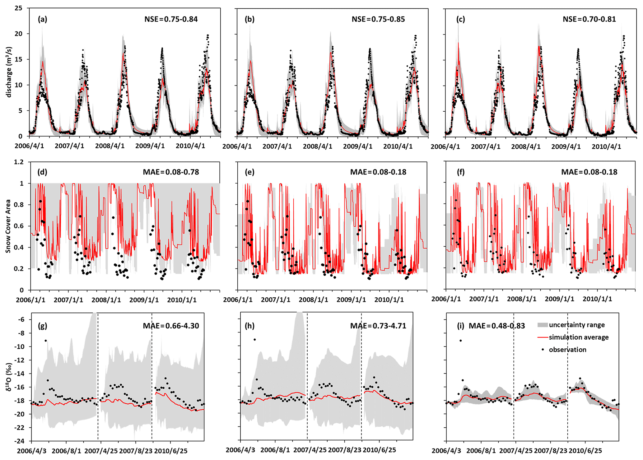
Figure 2Uncertainty ranges of simulations in the calibration period produced by the behavioral parameter sets of the single-objective (a, d, g), dual-objective (b, e, h) and triple-objective (c, f, i) calibration variants.
Figure 3a shows median value of the simulated daily inputs of water sources (rainfall, snowmelt and glacier melt) for the calibration period obtained by the behavioral parameter sets of the triple-objective variant. All the three water sources started to contribute to stream water around April. The volume of snowmelt peaked around June and then decreased rapidly in July as the catchment SCA decreased significantly. The volumes of rainfall and glacier melt peaked in mid-summer, which was the wettest and warmest period in the year. The fluctuations of the simulated δ18O of stream water in Fig. 3b are generally consistent with the varying contributions of these water sources to runoff. At the beginning of the wet season, δ18O of stream water increased rapidly in response to the dominance of the isotope-enriched precipitation. The δ18O of stream water began to decease in the late wet season, likely because of the reduced δ18O of precipitation reported as “temperature effect” (Dansgaard, 1964), which is mainly due to the effect of southwest monsoon (Yin et al., 2006), as well as the increased contributions of isotopic depleted glacier melt.
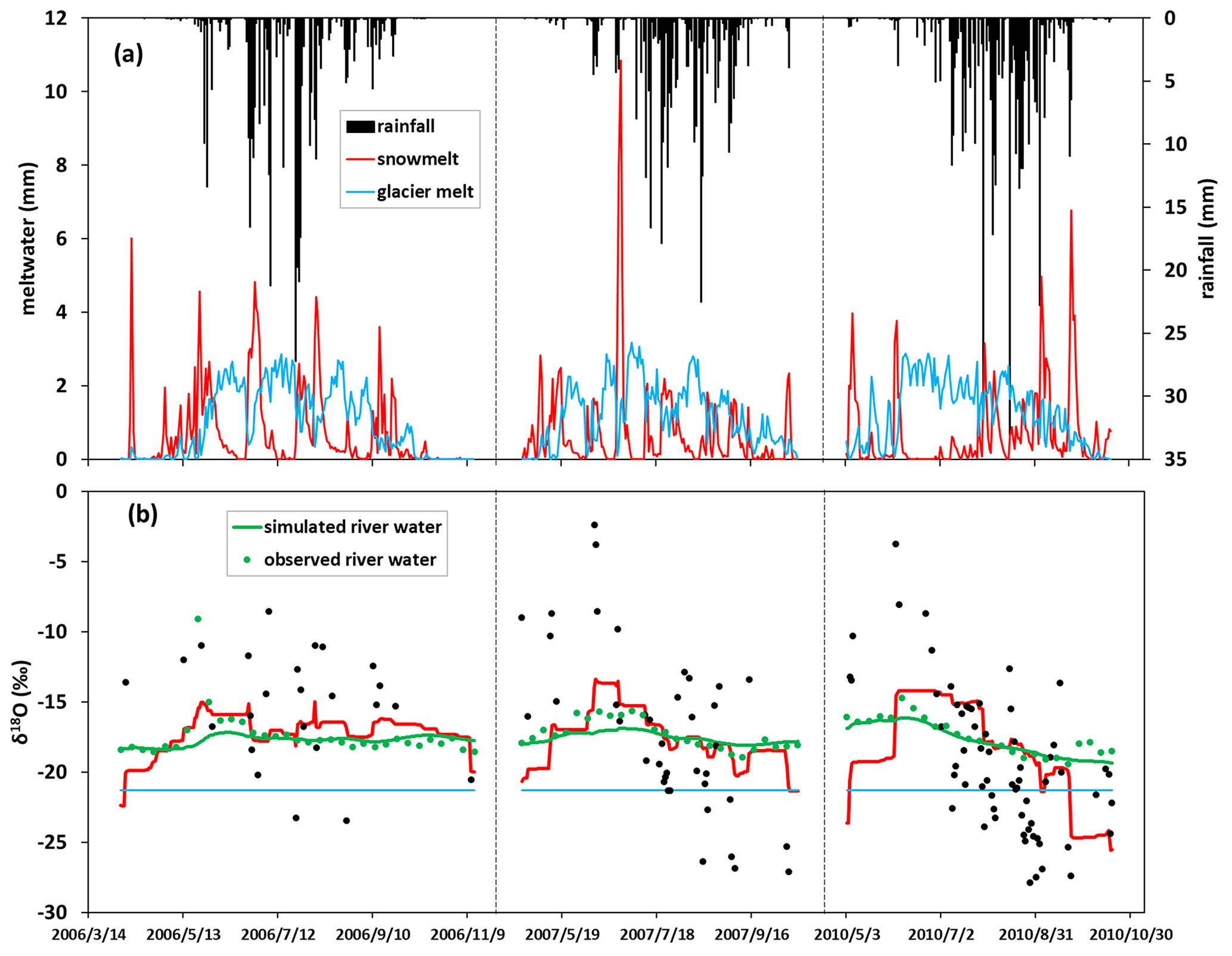
Figure 3Daily simulations of (a) each water source and (b) the corresponding isotopic compositions. The black points and red and blue lines in panel (b) mean the isotope composition of the water sources as represented by the corresponding color in panel (a).
3.2 Contributions of runoff components
The results of runoff component quantification reported in this section were based on the behavioral parameter sets of the three calibration variants. Table 4 and Fig. 4 show the proportions of water sources in the mean annual water input during 1 January 2007 to 31 December 2011. In all the three calibration variants rainfall provided most of the water quantity for runoff generation (44.2 % to 48.0 %) because of the high partition of rainfall (around 347 mm) in the annual precipitation (around 587 mm). The single-objective variant estimated the lowest proportion of snowmelt (19.7 %), because the simulation of SCA was not constrained in the calibration, leading to largely overestimated SCA in comparison to the MODIS SCA estimates due to less melting (Fig. 2d). The dual-objective variant estimated the highest proportion of glacier melt (33.8 %), resulting in a lower proportion of rainfall (44.2 %). Involving the calibration objective of isotope, the triple-objective variant estimated the lowest proportion of glacier melt (29.2 %) by rejecting the parameter sets that produced high contribution of glacier melt (as shown in Fig. 4), which will be discussed more in detailed in the discussion section. To be noted, despite above differences, is that the results of the three calibration variant were quite similar, with the maximum difference lower than 5 %. However, the uncertainties in the simulated water proportions decreased substantially with the increase of data that was involved in the calibration, showing as a decreasing uncertainty (12.4 % to 6.2 %, Table 4) and fewer outliers (Fig. 4), demonstrating considerable values of additional datasets for constraining the simulations of corresponding runoff-generation processes.
Table 4Average percentages of water sources in the annual water input for runoff generation.
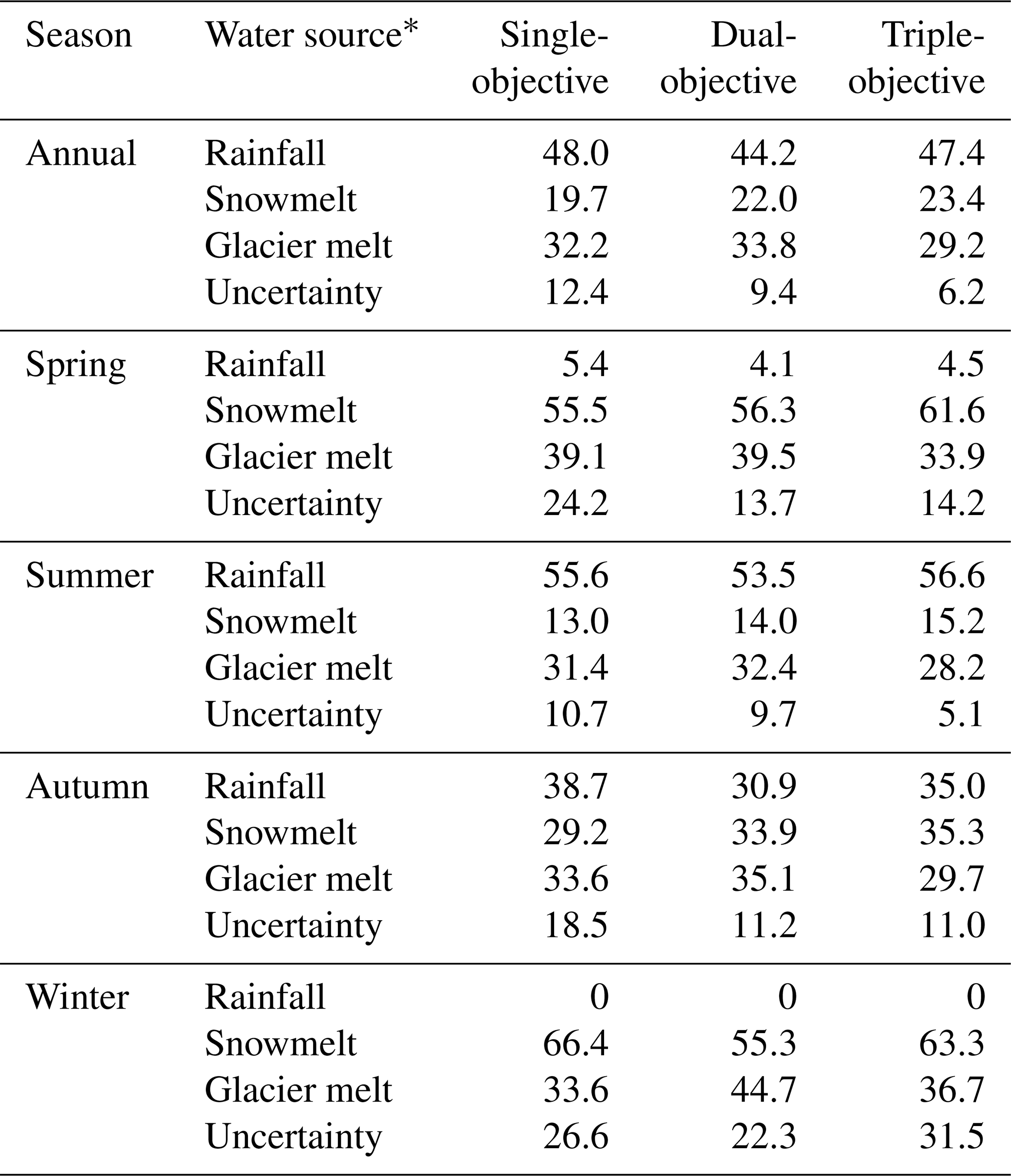
* The uncertainty of the contribution is defined as , where ER, EN and EG represent the standard deviations of the contributions of the water sources produced by the corresponding behavioral parameter sets. Subscripts R, S and G represent rainfall, snow meltwater and glacier meltwater, respectively.
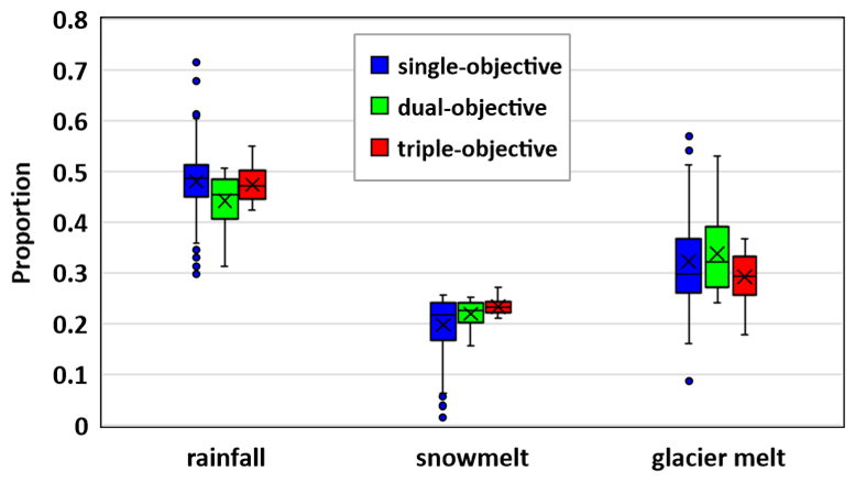
Figure 4Average proportion of different sources in the annual water input for runoff generation.
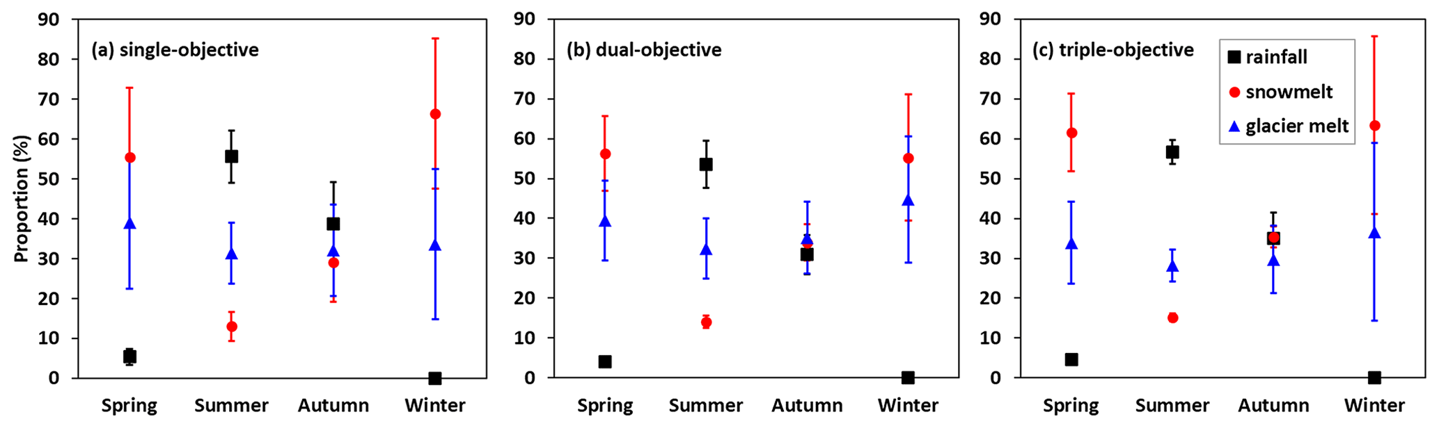
Figure 5Seasonal contributions of rainfall, snowmelt and glacier melt to total water input estimated by the (a) single-objective, (b) dual-objective and (c) triple-objective calibration variants. The error bars indicate the uncertainty ranges simulated by the corresponding behavior parameter sets.
Figure 5 and Table 4 compare the seasonal proportions of water sources in the total water input of the three calibration variants. The seasonal dominance of the water sources on runoff estimated by the three calibration variants are similar. In particular, the proportion of rainfall was large (around 55 %) in summer but small in winter when rainfall rarely occurred. Snowmelt and glacier melt dominated the total water input in winter with proportions of around 60 % and 40 %, respectively. The proportion of meltwater in summer was relatively low because of the dominance of rainfall during the summer monsoon. Snowmelt could only account for around 15 % in the total water input in summer because of the significantly reduced snowpack. The proportion of glacier melt was higher than that of snowmelt in summer because of the decreasing snow cover area. In the spring months, snowmelt and glacier melt contributed around 55 %–60 % and 35 %–30 % to the total water input, respectively, and rainfall provided the remaining 5 %. The glacier melt provided a steady contribution of around 30 %–40 % throughout the entire hydrological year. The seasonal proportions of water sources show slightly different values among the calibration variants. Specifically, the triple-objective calibration estimated not only the highest snowmelt and lowest glacier melt in the three seasons except winter but also the highest contribution of rainfall in summer (Fig. 5c), which was consistent with the lowest contribution of glacier melt in total water input estimated by triple-objective calibration. Single-objective calibration produced the highest contribution of rainfall in autumn and the highest contribution of snowmelt in winter (Fig. 5a). Although the contribution of water sources exhibited a large uncertainty in winter, and significant differences existed among the calibration variants, it had negligible effect on the annual result because of the extremely low contribution of water input during winter (< 1 %). The uncertainty ranges of the seasonal proportion during summer and autumn were obviously reduced by the triple-objective calibration (Fig. 5c).
Table 5 shows the contributions of runoff components to annual and seasonal runoff. Three calibration variants resulted in rather similar contributions of surface runoff and subsurface runoff (around 65 % and 35 %, respectively). Surface runoff was the dominant component in this catchment because of the large glacier-covered area (around 20%) and the large saturation area (around 20 %). The triple-objective calibration estimated relatively lowest surface runoff (64.9 %) and highest subsurface runoff (35.1 %). Surface runoff dominated streamflow during spring and summer (with proportions of around 65 % and 80 %, respectively), when large rainfall and snowmelt events occurred frequently and the catchment was rather wet. Subsurface runoff played a more important role during autumn, accounting for about 60 % of the runoff. The runoff in winter was dominated by baseflow because of the very rare water input events. Again, the triple-objective calibration resulted in lowest uncertainty ranges for the contributions of the runoff components compared to the other two calibration variants (4.1 % compared to 12.1 %). Isotope data used in the triple-objective variant provided additional constraints on the estimation of parameters controlling the generation of subsurface flow (such as KKA and KKD in Table 2) and the saturation area where surface runoff occurred (such as WM and B), thus constraining the partitioning between surface runoff and subsurface runoff.
Table 5Simulated contributions of runoff components to annual runoff.
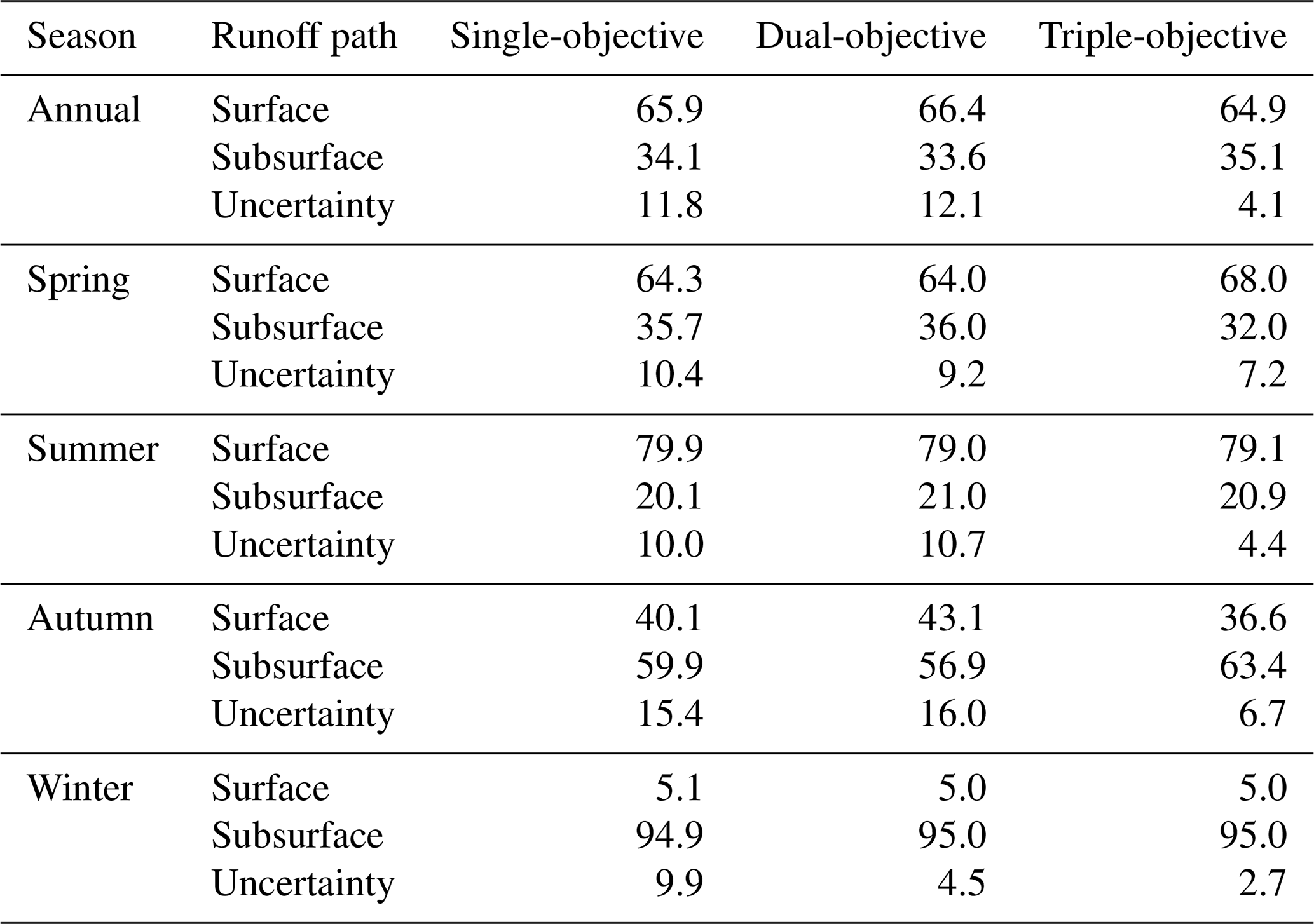
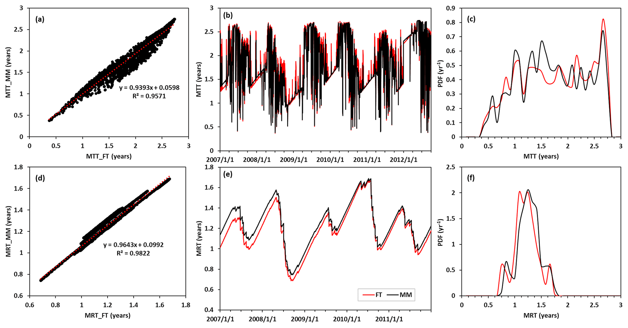
Figure 6Comparison between the MM and FT methods: scatterplots for daily (a) MTT and (d) MRT; time series of the daily (b) MTT and (e) MRT; and probability density functions of the daily (c) MTT and (f) MRT.
3.3 Estimations of water travel time and residence time
The travel time and residence time were estimated for the 5 water years (1 January 2007 to 31 December 2011) during the simulation period. The result produced by the best parameter set ((NSEdis= 0.72, MAESCA= 0.079, MAEiso= 0.484) was used to test the consistency between the two model-based methods. Based on the assumption that glacier melt water had an age of 1000 d, the backward MTT and MRT estimated by the MM (FT) method were 1.70 (1.72) and 1.22 (1.17) years, respectively. Figure 6 shows the comparison between the results of the MM and FT methods. As shown in Fig. 6a and d, there were strong correlation between the daily MTTs (MRTs) estimated by the two methods with a high correlation coefficient of 0.96 (0.98). The daily MTT and MRT series also showed similar temporal variability between the two methods as shown in Fig. 6b and e. The MRT increased steadily during dry season and decreased rapidly during wet season due to the recharge of young precipitation. The daily MTT also showed steady increasing trend during dry season but showed significant fluctuation during wet season because of the combined effect of young precipitation and old glacier meltwater. Figure 6c and e show the probability density function of the daily backward MTT and MRT produced by the two methods. The daily MTT had a large range from 0.42 to 2.75 years, with several peak density values at around 1, 1.5 and 2.67 years, including the influence of the multiple water sources with different ages. On the contrary, the daily MRT only had a narrow range from 0.75 to 1.75 years, with a significant peak value at around 1.25 years, similar to the MRT. Excluding the effect of glacier meltwater, the FT method estimated the precipitation-triggered backward MTT of runoff as 263 d, significantly smaller than the MRT, indicating the incomplete mixing in the catchment scale caused by the distributed modeling framework.
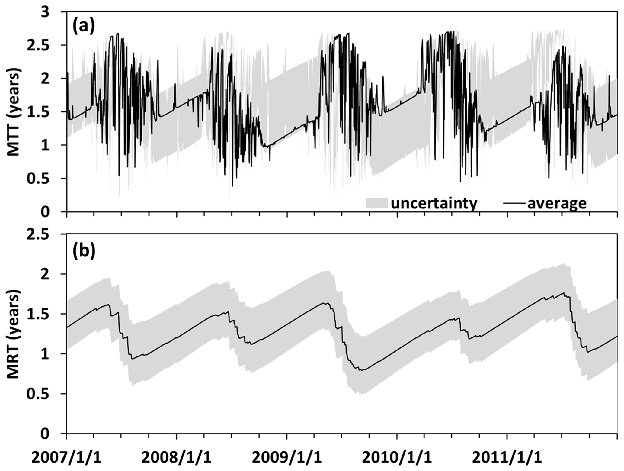
The lumped SW method estimated the MTT and MRT as 1.68 years (Ar and Ap were estimated as 0.58 and 6.19, respectively). Based on the average result of 19 behavioral parameter sets, the model-based methods estimated the MTT and MRT as 1.61 and 1.28, respectively. The two kinds of methods produced similar MTT, indicating the robustness of travel time estimation in this catchment. The precipitation-triggered MTT (shorter than 1 year) was significantly smaller than the MTT of total runoff estimated by the lumped method, indicating the effect of old glacier melt water. The glacier melt contributed to stream water through surface runoff directly and had no contribution to the water storage, leading to a smaller model-based MRT compared to MTT. The uncertainty of MTT and MRT estimation could be reflected by the range produced by the MM method by the 19 behavioral parameter sets as shown in Fig. 7. The standard deviation values of the estimated MTT and MRT were 74 and 79 d, respectively. The uncertainty range during June to August was relatively small (Fig. 7a), indicating that different behavioral parameters produced similar precipitation-triggered processes during the wet season, and the uncertainty mainly came from the large range of MRT, i.e., the age of water storage including soil water and groundwater.
Based on the best parameter set, the FT method tracked the transportation of precipitation and produced time-varying forward TTD, backward TTD and RTD. For simplicity, Fig. 8 shows the average distributions weighted by the precipitation amount (for forward TTD), runoff generation (for backward TTD) and water storage (for RTD). As shown in Fig. 8a and b, the forward and backward TTD were similar, behaving as a high proportion (∼0.3) of the youngest water, which was consistent with the high proportion of rapid surface runoff. The high proportion of young water led to a similar TTD form as the exponential model. The relative peaks of TTD were mainly around the travel time of integral years, indicating the influence of baseflow from groundwater, which were recharged by precipitation in the wet seasons of previous years. The simulated RTD was significantly different from the TTD, behaving as the low probability density of young water. The young water was mainly recharged by the infiltrating rainfall and snowmelt, which was negligible compared to the total water storage. Again, the difference between TTD and RTD indicated the incomplete mixing processes, behaving as affinity for young water due to the rapid flow pathways such as in surface runoff.

Figure 8The weighted average probability distributions of (a) forward TTD, (b) backward TTD and (c) RTD estimated by the FT method.
4.1 The values of tracer on constraining flow pathways and water storages in the hydrological model
This study developed a tracer-aided hydrological model and tested its behavior in a glacierized catchment. Because of the sampling difficulties on the Tibetan Plateau, the tracer data of the water sources (e.g., snow, glacier, groundwater) were rather limited compared to other tracer-aided modeling work (e.g., Ala-aho et al., 2017; He et al., 2019). Nonetheless, the model developed in this study performed well on producing the tracer signature of stream water, producing a tool for applying the tracer-aided method to the areas with limited tracer data. Although it is widely accepted that simple input–output tracer measurements provide limited insight into catchment function and that sampling source water components would be helpful (Birkel et al., 2014; Tetzlaff et al., 2014), the uncertainty of the model could still be reduced significantly by satisfying the output tracer signature (Delavau et al., 2017), especially in cold regions where hydrological processes were more complex. The fact that the model can simultaneously satisfy three calibration objectives over a long period gave confidence to the model realizations (McDonnell and Beven, 2014).
Our results indicate that involving the isotope in the calibration significantly reduced the uncertainty of quantifying the runoff components. To understand the role of isotope data on reducing the uncertainty, the results of the dual-objective calibration variant were analyzed for why some of the parameter sets behaved poorly on isotope simulation despite their good performance on discharge and snow simulation. Among the 117 behavioral parameter sets of dual-objective calibration, only 14 of them produced relatively good isotope simulations (MAEiso < 1.0). As shown in Fig. 9a and b, these 14 isotopic behavioral parameter sets produced the proportion of runoff component within a relatively smaller range (27.5 % to 38 % for glacier melt and 58 % to 75 % for surface runoff), while the 117 behavioral parameter sets produced a much larger variation (24 % to 53 % for glacier melt and 40 % to 90 % for surface runoff). This indicated that involving isotope data for model calibration helped to exclude some unreasonable proportions of runoff component. The distribution of scatter in Fig. 9a and b was similar, and the proportion of surface runoff had a strong correlation with the proportion of glacier melt as shown in Fig. 9c (because of the assumption that glacier melt contributed to surface runoff directly); thus, the mechanism that isotopes can reject unreasonable proportions was the same for water sources and runoff-generation processes. Fig. 9d shows the simulation range of δ18O of stream water by calibrated parameters that resulted in glacier melt proportion in the total water input higher than 40 %. The simulated isotopic signature showed strong fluctuations due to the high proportion of surface runoff with a larger time variation compared to the relatively steady signature of subsurface runoff. Also, the simulated isotopic values were significantly higher than the observations, which was mainly the result of the excessive isotopic fractionation due to the too much evaporation of surface water (Hindshaw et al., 2011; Wolfe et al., 2007). Figure 9e shows the simulation range by the parameters with proportion of surface runoff lower than 45 %. In contrast to scenarios with too high glacier melt, the simulated isotope signature showed small variation and the mean values were much lower than the observation. Our result also showed that the proportion of surface runoff and glacier melt tended to be higher when the NSEdis was higher, indicating that focusing on the simulation of integrated observation of discharge only will likely lead to overestimated surface runoff and glacier melt. These results indicated that the isotope data helped to constrain the quantifications of runoff components by (1) regulating the competition between rapid component with strong variation in isotope signatures (e.g., surface runoff) and slow component with relatively stable isotope signatures (e.g., subsurface runoff) to match the daily fluctuations of observed isotope signature of stream water and (2) controlling the isotopic fractionation by adjusting the evaporation to satisfy the observed isotopic value.
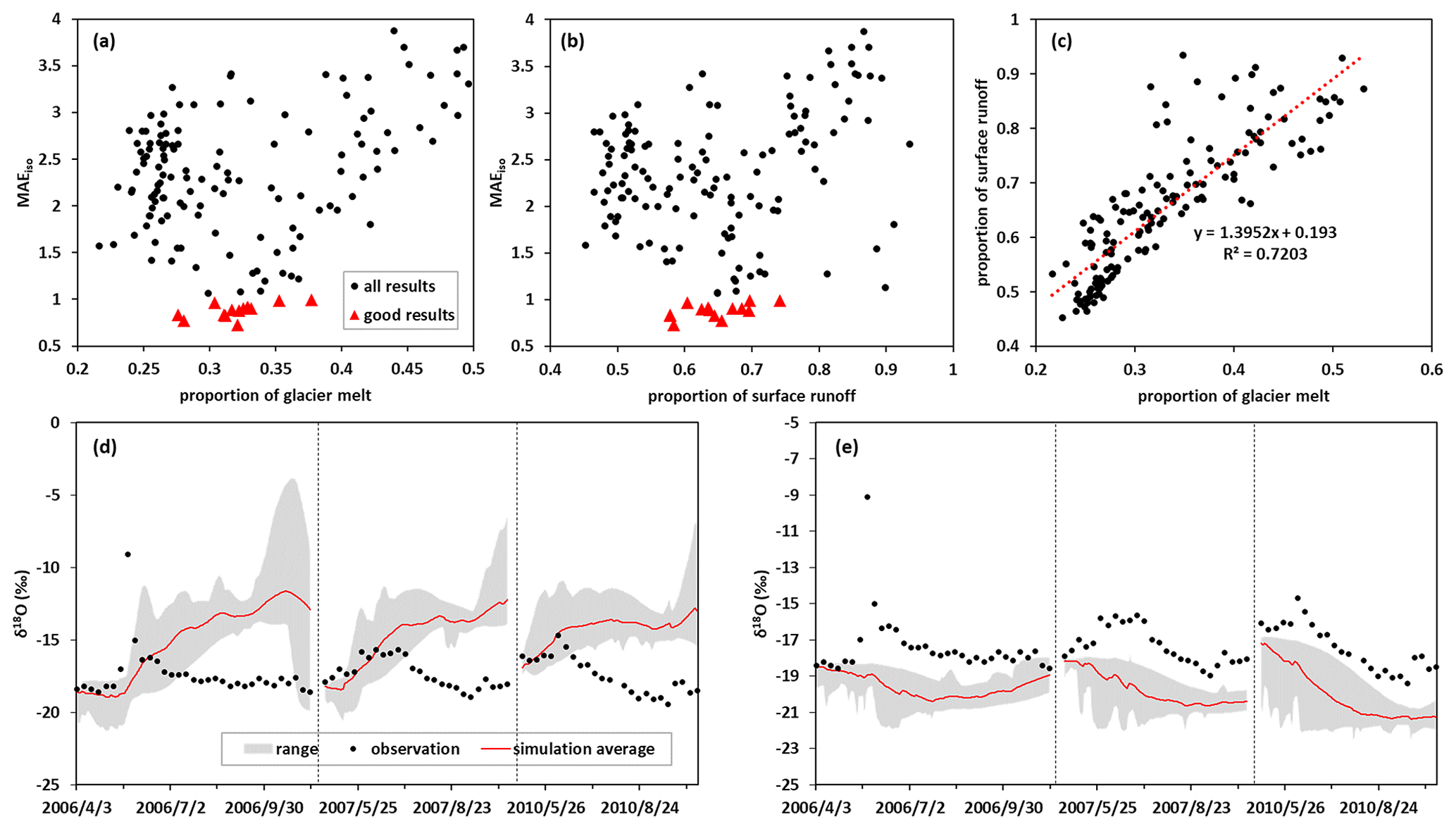
Figure 9The role of isotope calibration on constraining the proportion of runoff components. (a) The relationship between MAEiso and proportion of glacier melt. (b) The relationship between MAEiso and proportion of surface runoff. (c) The relationship between proportion of surface runoff and that of glacier melt. (d) The simulated isotope in stream water produced by the parameter sets estimating proportion of glacier melt higher than 40 %. (e) The simulated isotope in stream water produced by the parameter sets estimating proportion of surface runoff lower than 45 %.
Two model-based methods (MM and FT) were adopted to estimate travel time and residence time in this study, and they were verified by the result of lumped method (SW). Both MM and FT methods can estimate MTT and MRT, but FT provided more information including TTD and RTD, which was actually more of interest. The MM method has been used in several previous studies, including modeling work in snow-influenced basins (Ala-aho et al., 2017). Consequently, the results of FT and MM were compared in this study to ensure that the additional information provided by the FT method was reasonable. Our result indicated that the two model-based methods produced consistent results, which were also similar to the lumped method, indicating the robustness of MTT and MRT estimation through a tracer-aided model without defining any prior distribution functions.
Although significantly constraining the proportion of runoff component, the uncertainty ranges of simulated MTT and MRT, especially that during baseflow-dominant period (as shown in Fig. 7b), were still rather large, indicating that the estimation of groundwater age had a large uncertainty, which was similar to other model-based age estimation work (e.g., Ala-aho et al., 2017; van Huijgevoort et al., 2016). The isotope observations were mainly collected during the wet season when precipitation-triggered surface runoff played an important role in runoff generation; thus, this process was constrained relatively well by the isotope calibration, showing as the similar fluctuation of MTT during wet season produced by different parameter sets. Although the proportion of subsurface runoff was constrained, the storage volume of groundwater was poorly constrained because of the relatively simplified structure of the groundwater module of THREW model (Tian et al., 2006), which adopted a two-layer reservoir model to describe the processes of seepage and subsurface flow. Apart from involving more calibration objectives, improving the physical mechanism and the representation of hydrological processes is another important way to constrain the model behavior and reduce uncertainties.
4.2 Insight from MTT and MRT estimation
Based on the three MTT estimation methods, this study estimated the MTT and MRT as 1.7 and 1.2 years, respectively, reflecting the age of stream water and subsurface water storage in the catchment. Excluding the effect of aged glacier meltwater, the MTT of stream water fed by rainfall and snowmelt decreased to around 9 months. Ala-aho et al. (2017) estimated the median water ages of three snow influenced catchments located in the USA, Sweden and Scotland using the MM method as 11 months, 1.5 and 5 years, respectively. The water age had a rather wide range among different catchments, which mainly depends on the groundwater storage controlled by the topography and soil characteristics. The process where water travels through the subsurface pathway plays a comparable role with the snow accumulation process on the water age in snow influenced catchments. The significantly lower MTT and MRT estimated in this study than that of the three catchments in Ala-aho et al. (2017) can be mainly attributed to the large impermeable area on the glacier, leading to a large proportion of surface runoff with very short travel time.
The influence factors of the MTT and MRT were analyzed to better understand the hydrological processes in the catchment. The relationship between the daily travel times (including forward MTT, backward MTT and MRT) and the environmental factors (including simulated soil water content and meteorological factors) was analyzed in Fig. 10. The result shows the scatter diagrams between the factors with good correlation. MRT presented a strong negative correlation with the soil water content (Fig. 10a), which was consistent with the finding by Hrachowitz et al. (2013) and Heidbuechel et al. (2012) that the resident water age was sensitive to antecedent wetness and the water stored in subsurface storage. During dry season, the MRT became older as time went on, and the soil water content was decreasing due to the outflow of groundwater. The soil water content increased rapidly during wet season when precipitation occurred and recharged the groundwater, and the MRT became younger due to the recharge of young water. Backward MTT had a good relationship with both soil water (Fig. 10b) and precipitation amount (Fig. 10c). During the dry season when runoff was mainly baseflow, the age of stream water was similar to the groundwater and consequently controlled by the soil water content. During wet season, the backward MTT was largely dependent on the precipitation amount, because a large proportion of young precipitation event water contributed to stream water quickly through surface runoff pathway, leading to small MTT. This was also consistent with the result reported by Hrachowitz et al. (2013) and McMillan et al. (2012) that the water flux age was controlled by fast and slow processes under wetting-up and drying-up conditions. The forward MTT reflected the time that the input water took to travel through the catchment, showing good relationship with temperature (Fig. 10d). The negative correlation between forward MTT and temperature was mainly related to two processes, i.e., the snow accumulation and the evaporation. When the temperature was low, the precipitation was mainly in the form of snowfall, which cannot contribute to the stream quickly, resulting in a long travel time. On the contrary, the water would be exposed to intense evaporation when the temperature was high. Large proportion of precipitation event water left the catchment quickly by evaporation before infiltrating into groundwater and going through the long subsurface pathway, resulting in a short travel time. The negative relation between forward MTT and temperature indicated an accelerated water cycling process as a result of climate warming.
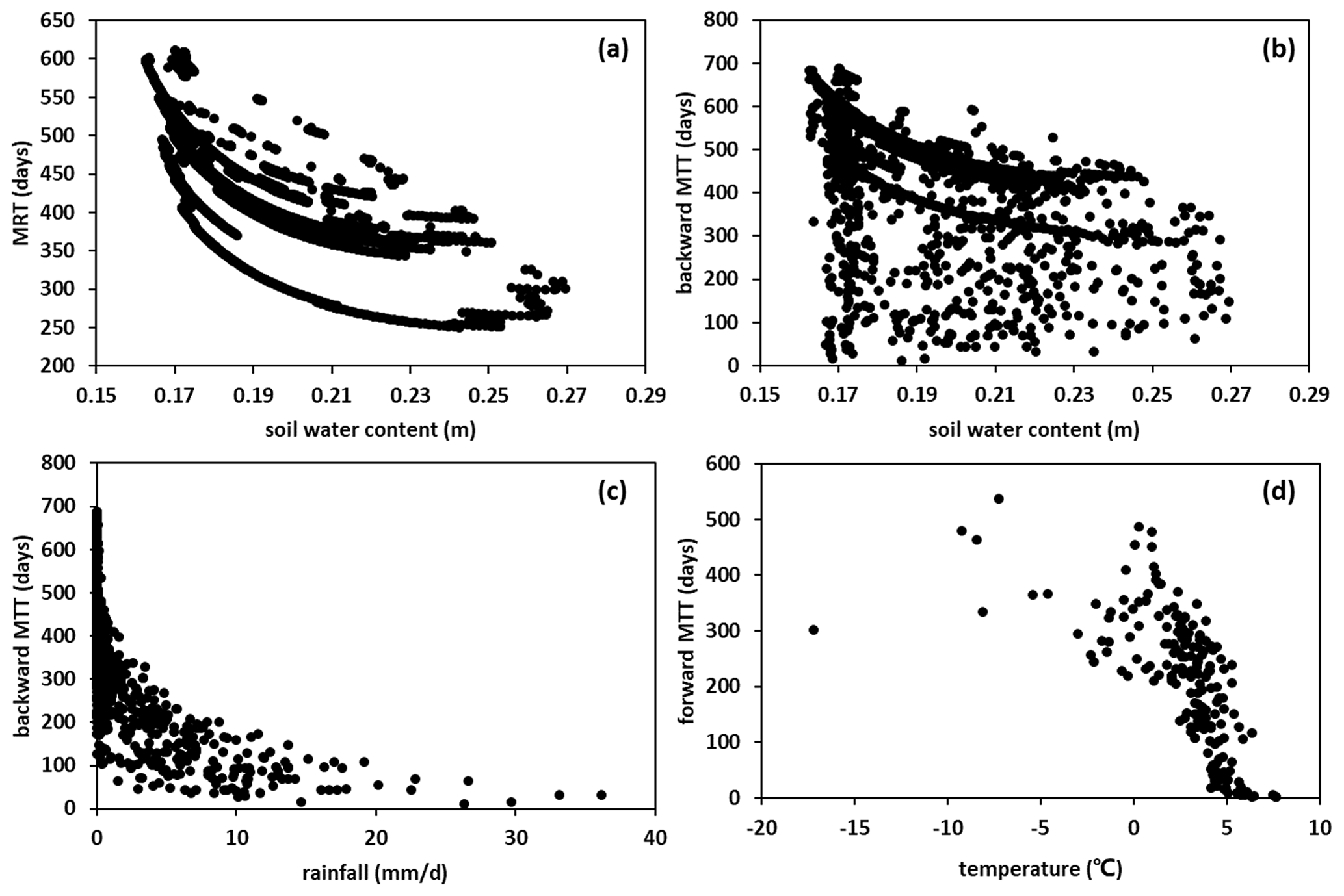
Figure 10The scatter diagrams between (a) MRT and soil water content, (b) backward MTT and soil water content, (c) backward MTT and rainfall, and (d) forward MTT and temperature.
4.3 Limitation and uncertainty
Multiple water sources brought difficulties to hydrological modeling in glacierized basins (Li et al., 2019). Focusing on the tracer transportation processes, the model developed in this study made some simplifications on the processes related to snow and glacier to make the model structure parsimonious. First, the snow accumulation and melting processes were simulated by a simple temperature-based method, which was relatively less of a physical mechanism compared to the energy-based methods (e.g., Pomeroy et al., 2007). Nonetheless, this method had an acceptable behavior and was widely used in studies of snow simulation (e.g., He et al., 2014), and the simulated SCA was validated by the MODIS data during the ablation period in this study. Second, the evolution of glacier thickness and area were not simulated in the model. Simplification of a constant glacier area likely led to an overestimation of the contribution of glacier melt to runoff, as the glacier cover area should get smaller due to the climate warming. However, this simplification should have a minor influence on the result, because the changes in glacier area were rather small in a short simulation period of 7 years.
The influence of calibration objective function was inadequately assessed in this study. Although the measurement units of NSEdis was different from the MAESCA and MAEiso, their values were of the same order of magnitude when the model performance was acceptable (similarly with He et al., 2019). Consequently, they were combined directly to reflect the simultaneous performance on the three objectives. Plenty of studies have developed methods to solve the problem of multiple objective calibration by introducing an integrated evaluation metric (e.g., Gupta et al., 2009; Shafii and Tolson, 2015) or giving weights to each objective (e.g., Tong et al., 2021). This study mainly aimed to evaluate the value of isotope data on improving the model behavior rather than developing a general calibration strategy; thus, the three evaluation metrics were added together with equal weights for simplification to represent the condition that all the three objectives were simulated well. Our main findings indicated that the results calibrated by discharge and isotope were more behavioral in many aspects than the results calibrated only by discharge. The potential influences of calibration metrics and methods on the finally optimized result still needed further exploration.
The lack of source water sampling made it difficult to fully validate the modeling result. Although the isotope signature of stream water was reproduced well, it cannot guarantee that the isotopic variations in groundwater and snowmelt were simulated correctly. The quantification of runoff components was also hard to verified. The end-member method cannot be applied as a reference due to the lack of water source tracer data. A previous study of snow cover and runoff modeling work in the same basin (Zhang et al., 2015) provided a potential reference. That work indicated that the contribution of rainfall, snowmelt and glacier melt in 2006 were 30 %, 10 % and 60 %, respectively, which was markedly different from the result of this study. The runoff simulation in Zhang et al. (2015) was conducted by a simplified conceptual model with limited physical mechanism, which did not consider the processes of subsurface runoff and evaporation. And the glacier melt runoff coefficient (the ratio of glacier melt runoff to the total glacier melt) estimated by that study was very small (0.182), indicating that a large proportion of glacier melt did not contribute to the surface runoff directly, which is inconsistent with the common assumption in previous studies (e.g., Seibert et al., 2018; Schaefli et al., 2005). The extremely low glacier melt runoff coefficient might lead to overestimation of the contribution of glacier melt. The significant differences between the two studies mainly resulted from the difference of model structure. Intensive source water sampling together with systematic glacier observation might improve the behavior of hydrological models in glacierized basins and help us better understand the runoff processes.
In glacierized basins where glacier meltwater played an important role on runoff generation, the objectives of the three MTT estimation methods were different. The total runoff could be divided into precipitation-triggered runoff (including rainfall runoff and snowfall-snowmelt runoff) and glacier melt runoff. Considering that glacier was also formed by the precipitation over past years, the lumped SW method should have reflected both runoff processes, because it was based on the tracer data of precipitation and total runoff. The two model-based methods mainly focused on the precipitation-triggered runoff, because the glacier revolution process was simplified in the model. The MTT estimation of total runoff should be based on the assumed MTT of glacier melt water. In this study, assuming the MTT of glacier melt as 1000 d, the model-based results were similar to the SW method, indicating that the assumption of glacier melt MTT was appropriate, which was actually misleading. The timescale of glacier update was much longer than this assumed value, because the glacier generally took decades to hundreds of years to move from accumulation zone to ablation zone (Soncini et al., 2015; Yao et al., 2012). The good agreement among the three methods indicates that the SW method significantly underestimated the age of glacier. This was mainly due to the limited applicable timescale of stable isotope in water. It was reported that seasonal the cycle of stable isotopes in precipitation was most useful for inferring relatively short travel time of 2–4 years (McGuire and McDonnell, 2006; Sprenger et al., 2019; Stewart et al., 2010). The assumed glacier melt MTT of 1000 d was within this range; thus, the similar result of the three methods could verify the model representation of the precipitation-triggered runoff process, and the cross validation between the MM and FT methods further enhanced the robustness of the travel time estimation. Consequently, we can expect that if a tracer suitable for longer travel time (e.g., 14C) was used to estimate the proper MTT of total runoff, we could better infer the age of water according to the model-based estimation of precipitation-triggered runoff MTT.
A tracer module was integrated into the THREW hydrological model to constrain the various runoff processes, and it was tested in a glacierized catchment on the Tibetan Plateau. Measurements of oxygen stable isotopes of the stream water were used to calibrate the model parameters, in addition to the observations of discharge and MODIS SCA. The behaviors of the model, especially the quantifications of runoff components, were compared among the calibration variants with different objectives to test the value of isotope data on constraining the model parameters. A lumped method (SW) and two model-based methods (MM and FT) were applied to estimate the water travel time in the study basin. Our main findings are the following. (1) The THREW-t model performed well on simultaneously reproducing the variations in discharge, snow cover area, and the isotopic composition of stream water, despite a small water sample number of precipitation was available to provide isotope input data. (2) The contributions of rainfall, snowmelt and glacier melt to the annual runoff were quantified as 47.4 %, 23.4 % and 29.2 %. Surface runoff (contributing around 64.9 %) was more dominant than subsurface flow in the annual runoff. Calibration with isotope data significantly reduced the uncertainties by regulating the competition between rapid and slow runoff components to fit the variation in observed isotope signature, and resulted in more plausible quantifications of contributions of runoff components to seasonal runoff. (3) The estimated MTT of model-based methods MM and FT met well with that of a sine-wave lumped parameter method, indicating the robustness of travel time estimation benefiting from the use of water isotope data. The precipitation-triggered MTT was significantly shorter than the MTT of total runoff, indicating the effect of old glacier meltwater. The MRT was longer than precipitation-triggered MTT, indicating the catchment-scale incomplete mixing processes and the affinity for young water due to the rapid flow pathways such as runoff on the impermeable glacier surface. The temporal variation in MTT and MRT was dependent on the catchment wetness conditions and meteorological factors.
The isotope data and the code of the THREW-t model used in this study are available by contacting the authors.
YN, ZH and FT conceived the idea; LT provided the observation data; YN, FT, LT and ZH conducted analysis; LS provided comments on the analysis; and all the authors contributed to writing and revisions.
The authors declare that they have no conflict of interest.
Publisher's note: Copernicus Publications remains neutral with regard to jurisdictional claims in published maps and institutional affiliations.
This research has been supported by the National Natural Science Foundation of China (grant nos. 92047301 and 91647205).
This paper was edited by Lixin Wang and reviewed by two anonymous referees.
Ala-aho, P., Tetzlaff, D., McNamara, J. P., Laudon, H., and Soulsby, C.: Using isotopes to constrain water flux and age estimates in snow-influenced catchments using the STARR (Spatially distributed Tracer-Aided Rainfall–Runoff) model, Hydrol. Earth Syst. Sci., 21, 5089–5110, https://doi.org/10.5194/hess-21-5089-2017, 2017.
Benettin, P. and Bertuzzo, E.: tran-SAS v1.0: a numerical model to compute catchment-scale hydrologic transport using StorAge Selection functions, Geosci. Model Dev., 11, 1627–1639, https://doi.org/10.5194/gmd-11-1627-2018, 2018.
Beven, K. and Freer, J.: Equifinality, data assimilation, and uncertainty estimation in mechanistic modelling of complex environmental systems using the GLUE methodology, J. Hydrol., 249, 11–29, https://doi.org/10.1016/S0022-1694(01)00421-8, 2001.
Birkel, C., Tetzlaff, D., Dunn, S. M., and Soulsby, C.: Using time domain and geographic source tracers to conceptualize streamflow generation processes in lumped rainfall-runoff models, Water Resour. Res., 47, W02515, https://doi.org/10.1029/2010WR009547, 2011.
Birkel, C., Soulsby, C., and Tetzlaff, D.: Developing a consistent process-based conceptualization of catchment functioning using measurements of internal state variables, Water Resour. Res., 50, 3481–3501, https://doi.org/10.1002/2013WR014925, 2014.
Botter, G., Bertuzzo, E., and Rinaldo, A.: Catchment residence and travel time distributions: the master equation, Geophys. Res. Lett., 38, L11403, https://doi.org/10.1029/2011GL047666, 2011.
Bowen, G. J., Cai, Z., Fiorella, R. P., and Putman, A. L.: Isotopes in the water cycle: regional-to global-scale patterns and applications, Annu. Rev. Earth Planet. Sci., 47, 453–479, https://doi.org/10.1146/annurev-earth-053018-060220, 2019.
Capell, R., Tetzlaff, D., and Soulsby, C.: Can time domain and source area tracers reduce uncertainty in rainfall-runoff models in larger heterogeneous catchments?, Water Resour. Res., 48, W09544, https://doi.org/10.1029/2011WR011543, 2012.
Chen, X., Long, D., Hong, Y., Zeng, C., and Yan, D.: Improved modeling of snow and glacier melting by a progressive two-stage calibration strategy with grace and multisource data: how snow and glacier meltwater contributes to the runoff of the upper brahmaputra river basin?, Water Resour. Res., 53, 2431–2466, https://doi.org/10.1002/2016WR019656, 2017.
Dansgaard, W.: Stable isotopes in precipitation, Tellus, 16, 436–468, 1964.
Delavau, C. J., Stadnyk, T., and Holmes, T.: Examining the impacts of precipitation isotope input (δ18Oppt) on distributed, tracer-aided hydrological modelling, Hydrol. Earth Syst. Sci., 21, 2595–2614, https://doi.org/10.5194/hess-21-2595-2017, 2017.
Didan, K.: MOD13A3 MODIS/Terra vegetation Indices Monthly L3 Global 1km SIN Grid V006, NASA EOSDIS Land Processes DAAC [data set], https://doi.org/10.5067/MODIS/MOD13A3.006, 2015.
Dou, Y., Chen, X., Bao, A., and Li, L.: The simulation of snowmelt runoff in the ungauged kaidu river basin of tianshan mountains, china, Environ. Earth Sci., 62, 1039–1045, https://doi.org/10.1007/s12665-010-0592-5, 2011.
Duethmann, D., Peters, J., Blume, T., Vorogushyn, S., and Güntner, A.: The value of satellite-derived snow cover images for calibrating a hydrological model in snow-dominated catchments in Central Asia, Water Resour. Res., 50, 2002–2021, https://doi.org/10.1002/2013WR014382, 2014.
Duethmann, D., Bolch, T., Farinotti, D., Kriegel, D., Vorogushyn, S., Merz, B., Pieczonka, T., Jiang, T., Su, B., and Güntner, A.: Attribution of streamflow trends in snow and glacier melt-dominated catchments of the Tarim River, Central Asia, Water Resour. Res., 51, 4727–4750, https://doi.org/10.1002/2014WR016716, 2015.
Eriksson, D., Bindel, D., and Shoemaker, C.: Dme65/Pysot: V0.1.35, Zenodo [code], https://doi.org/10.5281/zenodo.569554, 2017.
Finger, D., Vis, M., Huss, M., and Seibert, J.: The value of multiple data set calibration versus model complexity for improving the performance of hydrological models in mountain catchments, Water Resour. Res., 51, 1939–1958, https://doi.org/10.1002/2014WR015712, 2015.
Gao, J., Tian, L., and Liu, Y.: Oxygen isotope variation in the water cycle of the Yamdrok-tso Lake Basin in southern Tibetan Plateau, Chinese Sci. Bull., 54, 2758–2765, 2009.
Garvelmann, J., Warscher, M., Leonhardt, G., Franz, H., Lotz, A., and Kunstmann, H.: Quantification and characterization of the dynamics of spring and stream water systems in the berchtesgaden alps with a long-term stable isotope dataset, Environ. Earth Sci., 76, 766, https://doi.org/10.1007/s12665-017-7107-6, 2017.
Gat, J. R.: Oxygen and hydrogen isotopes in the hydrologic cycle, Annu. Rev. Earth Pl. Sc., 24, 225–262, https://doi.org/10.1146/annurev.earth.24.1.225, 1996.
Gupta, H. V., Kling, H., Yilmaz, K. K., and Martinez, G. F.: Decomposition of the mean squared error and nse performance criteria: implications for improving hydrological modelling, J. Hydrol., 377, 80–91, https://doi.org/10.1016/j.jhydrol.2009.08.003, 2009.
Hall, D. K. and Riggs, G. A.: MODIS/Terra Snow Cover 8-Day L3 Global 500m SIN Grid, Version 6, NASA National Snow and Ice Data Center Distributed Active Archive Center [data set], https://doi.org/10.5067/MODIS/MOD10A2.006, 2016.
Harman, C. J.: Age-ranked storage-discharge relations: a unified description of spatially lumped flow and water age in hydrologic systems, Water Resour. Res., 55, 1567–1575, https://doi.org/10.1029/2017WR022304, 2019.
Harman, C. J. and Kim, M.: An efficient tracer test for time-variable transit time distributions in periodic hydrodynamic systems, Geophys. Res. Lett., 41, 1567–1575, https://doi.org/10.1002/2013GL058980, 2014.
He, Z. H., Parajka, J., Tian, F. Q., and Blöschl, G.: Estimating degree-day factors from MODIS for snowmelt runoff modeling, Hydrol. Earth Syst. Sci., 18, 4773–4789, https://doi.org/10.5194/hess-18-4773-2014, 2014.
He, Z. H., Tian, F. Q., Gupta, H. V., Hu, H. C., and Hu, H. P.: Diagnostic calibration of a hydrological model in a mountain area by hydrograph partitioning, Hydrol. Earth Syst. Sci., 19, 1807–1826, https://doi.org/10.5194/hess-19-1807-2015, 2015.
He, Z., Vorogushyn, S., Unger-Shayesteh, K., Gafurov, A., Kalashnikova, O., Omorova, E., and Merz, B.: The value of hydrograph partitioning curves for calibrating hydrological models in glacierized basins, Water Resour. Res., 54, 2336–2361, https://doi.org/10.1002/2017WR021966, 2018.
He, Z., Unger-Shayesteh, K., Vorogushyn, S., Weise, S. M., Kalashnikova, O., Gafurov, A., Duethmann, D., Barandun, M., and Merz, B.: Constraining hydrological model parameters using water isotopic compositions in a glacierized basin, central asia, J. Hydrol., 571, 332–348, https://doi.org/10.1016/j.jhydrol.2019.01.048, 2019.
He, Z., Unger-Shayesteh, K., Vorogushyn, S., Weise, S. M., Duethmann, D., Kalashnikova, O., Gafurov, A., and Merz, B.: Comparing Bayesian and traditional end-member mixing approaches for hydrograph separation in a glacierized basin, Hydrol. Earth Syst. Sci., 24, 3289–3309, https://doi.org/10.5194/hess-24-3289-2020, 2020.
Heidbuechel, I., Troch, P. A., Lyon, S. W., and Weiler, M.: The master transit time distribution of variable flow systems, Water Resour. Res., 48, 6520, https://doi.org/10.1029/2011WR011293, 2012.
Hindshaw, R. S., Tipper, E. T., Reynolds, B. C., Lemarchand, E., Wiederhold, J. G., Magnusson, J., Bernasconi, S. M., Kretzschmar, R., and Bourdon, B.: Hydrological control of stream water chemistry in a glacial catchment (Damma Glacier, Switzerland), Chem. Geol., 285, 215–230, https://doi.org/10.1016/j.chemgeo.2011.04.012, 2011.
Hrachowitz, M., Savenije, H., Bogaard, T. A., Tetzlaff, D., and Soulsby, C.: What can flux tracking teach us about water age distribution patterns and their temporal dynamics?, Hydrol. Earth Syst. Sci., 17, 533–564, https://doi.org/10.5194/hess-17-533-2013, 2013.
Immerzeel, W. W., Van Beek, L. P., and Bierkens, M. F.: Climate change will affect the Asian water towers, Science, 328, 1382–1385, https://doi.org/10.1126/science.1183188, 2010.
Immerzeel, W. W., Pellicciotti, F., and Bierkens, M. F. P.: Rising river flows throughout the twenty-first century in two Himalayan glacierized watersheds, Nat. Geosci. 6, 742–745, https://doi.org/10.1038/ngeo1896, 2013.
Kirchner, J. W.: Aggregation in environmental systems – Part 1: Seasonal tracer cycles quantify young water fractions, but not mean transit times, in spatially heterogeneous catchments, Hydrol. Earth Syst. Sci., 20, 279–297, https://doi.org/10.5194/hess-20-279-2016, 2016.
Kong, Y. and Pang, Z.: Evaluating the sensitivity of glacier rivers to climate change based on hydrograph separation of discharge, J. Hydrol. 434, 121–129, https://doi.org/10.1016/j.jhydrol.2012.02.029, 2012.
Kong, Y., Wang, K., Pu, T., and Shi, X.: Nonmonsoon precipitation dominates groundwater recharge beneath a monsoon-affected glacier in Tibetan Plateau, J. Geophys. Res.-Atmos., 124, 10913–10930, https://doi.org/10.1029/2019JD030492, 2019.
Konz, M. and Seibert, J.: On the value of glacier mass balances for hydrological model calibration, J. Hydrol., 385, 238–246, https://doi.org/10.1016/j.jhydrol.2010.02.025, 2010.
Li, Z., Feng, Q., Li, Z., Yuan, R., Gui, J., and Lv, Y.: Climate background, fact and hydrological effect of multiphase water transformation in cold regions of the western china: a review, Earth Sci. Rev., 190, 33–57, https://doi.org/10.1016/j.earscirev.2018.12.004, 2019.
Liu, S.: The second glacier inventory dataset of China (version 1.0) (2006–2011), National Tibetan Plateau Data Center [data set], https://doi.org/10.3972/glacier.001.2013.db, 2012.
Liu, Z., Tian, L., Yao, T., Gong, T., Yin, C., and Yu, W.: Temporal and spatial variations of δ18O in precipitation of the Yarlung Zangbo River Basin, J. Geogr. Sci., 17, 317–326, https://doi.org/10.1007/s11442-007-0317-1, 2007.
Luo, Y., Wang, X., Piao, S., Sun, L., Ciais, P., Zhang, Y., Ma, C., Gan, R., and He, C.: Contrasting streamflow regimes induced by melting glaciers across the Tien Shan – Pamir – North Karakoram, Sci. Rep.-UK, 8, 16470, https://doi.org/10.1038/s41598-018-34829-2, 2018.
Lutz, A. F., Immerzeel, W. W., Shrestha, A. B., and Bierkens, M. F. P.: Consistent increase in high asia's runoff due to increasing glacier melt and precipitation, Nat. Clim. Change, 4, 587–592, https://doi.org/10.1038/NCLIMATE2237, 2014.
Lutz, A. F., Immerzeel, W. W., Kraaijenbrink, P. D. A., Shrestha, A. B., and Bierkens, M. F. P.: Climate Change Impacts on the Upper Indus Hydrology: Sources, Shifts and Extremes, PLOS ONE, 11, e0165630, https://doi.org/10.1371/journal.pone.0165630, 2016.
Marques, J. E., Samper, J., Pisani, B., Alvares, D., Carvalho, J. M., Chamine, H. I., Marques, J. M., Vieira, G. T., Mora, C., and Sodre Borges, F.: Evaluation of water resources in a high-mountain basin in Serra da Estrela, Central Portugal, using a semi-distributed hydrological model, Environ. Earth Sci., 62, 1219–1234, https://doi.org/10.1007/s12665-010-0610-7, 2011.
McDonnell, J. J. and Beven, K.: Debates – The future of hydrological sciences: A (common) path forward? A call to action aimed at understanding velocities, celerities and residence time distributions of the headwater hydrograph, Water Resour. Res., 50, 5342–5350, https://doi.org/10.1002/2013WR015141, 2014.
McGuire, K. J. and McDonnell, J. J.: A review and evaluation of catchment transit time modeling, J. Hydrol., 330, 543–563, https://doi.org/10.1016/j.jhydrol.2006.04.020, 2006.
McMillan, H., Tetzlaff, D., Clark, M., and Soulsby, C.: Do time-variable tracers aid the evaluation of hydrological model structure? A multimodel approach, Water Resour. Res., 48, W05501, https://doi.org/10.1029/2011WR011688, 2012.
Mi, D., Xie, Z., and Luo, R.: China Glacier Information System XI: Gangze Water System, Xi'an, Atlas Press, China, 2001.
Miller, J. D., Immerzeel, W. W., and Rees, G.: Climate change impacts on glacier hydrology and river discharge in the Hindu Kush–Himalayas, Mt. Res. Dev., 32, 461–467, https://doi.org/10.1659/MRD-JOURNAL-D-12-00027.1, 2012.
Myneni, R., Knyazikhin, Y., and Park, T.: MOD15A2H MODIS/Terra Leaf Area Index/FPAR 8-Day L4 Global 500 m SIN Grid V006, NASA EOSDIS Land Processes DAAC [data set], https://doi.org/10.5067/MODIS/MOD15A2H.006, 2015.
Nash, J. E. and Sutcliffe, J. V.: River flow forecasting through conceptual models part I – A discussion of principles, J. Hydrol., 10, 282–290, https://doi.org/10.1016/0022-1694(70)90255-6, 1970.
Nepal, S., Krause, P., Flügel, W., Fink, M., and Fischer, C.: Understanding the hydrological system dynamics of a glaciated alpine catchment in the Himalayan region using the J2000 hydrological model, Hydrol. Process., 28, 1329–1344, https://doi.org/10.1002/hyp.9627, 2014.
Nepal, S., Zheng, H., Penton, D. J., and Neumann, L. E.: Comparative performance of GR4JSG and J2000 hydrological models in the Dudh Koshi catchment of the Himalayan region, in: MODSIM2015, 21st International Congress on Modelling and Simulation, Gold Coast, Australia, 29 November–4 December 2015, 2395–2401, 2015.
Parajka, J. and Blöschl, G.: The value of modis snow cover data in validating and calibrating conceptual hydrologic models, J. Hydrol., 358, 240–258, https://doi.org/10.1016/j.jhydrol.2008.06.006, 2008.
Pomeroy, J. W., Gray, D. M., Brown, T., Hedstrom, N. R., Quinton, W. L., Granger, R. J., and Carey, S. K.: The cold regions hydrological model: a platform for basing process representation and model structure on physical evidence, Hydrol. Process., 21, 2650–2667, https://doi.org/10.1002/hyp.6787, 2007.
Remondi, F., Kirchner, J. W., Burlando, P., and Fatichi, S.: Water flux tracking with a distributed hydrological model to quantify controls on the spatiotemporal variability of transit time distributions, Water Resour. Res., 54, 3081–3099, https://doi.org/10.1002/2017WR021689, 2018.
Schaefli, B. and Huss, M.: Integrating point glacier mass balance observations into hydrologic model identification, Hydrol. Earth Syst. Sci., 15, 1227–1241, https://doi.org/10.5194/hess-15-1227-2011, 2011.
Schaefli, B., Hingray, B., Niggli, M., and Musy, A.: A conceptual glacio-hydrological model for high mountainous catchments, Hydrol. Earth Syst. Sci., 9, 95–109, https://doi.org/10.5194/hess-9-95-2005, 2005.
Seibert, J., Vis, M. J. P., Kohn, I., Weiler, M., and Stahl, K.: Technical note: Representing glacier geometry changes in a semi-distributed hydrological model, Hydrol. Earth Syst. Sci., 22, 2211–2224, https://doi.org/10.5194/hess-22-2211-2018, 2018.
Shafii, M. and Tolson, B. A.: Optimizing hydrological consistency by incorporating hydrological signatures into model calibration objectives, Water Resour. Res., 51, 3796–3814, https://doi.org/10.1002/2014WR016520, 2015.
Siderius, C., Biemans, H., Wiltshire, A., Rao, S., Franssen, W. H. P., Kumar, P., Gosain, A. K., Vliet, M. T. H. Van, and Collins, D. N.: Snowmelt contributions to discharge of the Ganges, Sci. Total Environ., 468–469, S93–S101, https://doi.org/10.1016/j.scitotenv.2013.05.084, 2013.
Son, K. and Sivapalan, M.: Improving model structure and reducing parameter uncertainty in conceptual water balance models through the use of auxiliary data, Water Resour. Res., 43, W01415, https://doi.org/10.1029/2006WR005032, 2007.
Soncini, A., Bocchiola, D., Confortola, G., Bianchi, A., Rooso, R., Mayer, C., Lambrecht, A., Palazzi, E., Smiraglia, C., and Diolaiuti, G.: Future hydrological regimes in the upper indus basin: a case study from a high-altitude glacierized catchment, J. Hydrometeorol., 16, 306–326, https://doi.org/10.1175/JHM-D-14-0043.1, 2015.
Soulsby, C., Birkel, C., Geris, J., Dick, J., Tunaley, C., and Tetzlaff, D.: Stream water age distributions controlled by storage dynamics and nonlinear hydrologic connectivity: Modeling with high-resolution isotope data, Water Resour. Res., 51, 7759–7776, https://doi.org/10.1002/2015WR017888, 2015.
Sprenger, M., Stumpp, C., Weiler, M., Aeschbach, W., Allen, S. T., Benettin, P., Dubbert, M., Hartmann, A., Hrachowitz, M., Kirchner, J. W., McDonnell, J. J., Orlowski, N., Penna, D., Pfahl, S., Rinderer, M., Rodriguez, N., Schmidt, M., and Werner, C.: The demographics of water: a review of water ages in the critical zone, Rev. Geophys., 57, 800–834, https://doi.org/10.1029/2018RG000633, 2019.
Stadnyk, T. A. and Holmes, T. L.: On the value of isotope-enabled hydrological model calibration, Hydrolog. Sci. J., 65, 1525–1538, https://doi.org/10.1080/02626667.2020.1751847, 2020.
Stewart, M. K., Morgenstern, U., and Mcdonnell, J. J.: Truncation of stream residence time: how the use of stable isotopes has skewed our concept of streamwater age and origin, Hydrol. Process., 24, 1646–1659, https://doi.org/10.1002/hyp.7576, 2010.
Terzer, S., Wassenaar, L. I., Araguás-Araguás, L. J., and Aggarwal, P. K.: Global isoscapes for δ18O and δ2H in precipitation: improved prediction using regionalized climatic regression models, Hydrol. Earth Syst. Sci., 17, 4713–4728, https://doi.org/10.5194/hess-17-4713-2013, 2013.
Tetzlaff, D., Birkel, C., Dick, J., Geris, J., and Soulsby, C.: Storage dynamics in hydropedological units control hillslope connectivity, runoff generation, and the evolution of catchment transit time distributions, Water Resour. Res., 50, 969–985, https://doi.org/10.1002/2013WR014147, 2014.
Tian, F., Hu, H., Lei, Z., and Sivapalan, M.: Extension of the Representative Elementary Watershed approach for cold regions via explicit treatment of energy related processes, Hydrol. Earth Syst. Sci., 10, 619–644, https://doi.org/10.5194/hess-10-619-2006, 2006.
Tian, F., Li, H., and Sivapalan, M.: Model diagnostic analysis of seasonal switching of runoff generation mechanisms in the Blue River basin, Oklahoma, J. Hydrol., 418, 136–149, https://doi.org/10.1016/j.jhydrol.2010.03.011, 2012.
Tian, F., Xu, R., Nan, Y., Li, K., and He, Z.: Quantification of runoff components in the Yarlung Tsangpo River using a distributed hydrological model, Adv. Water Sci., 31, 324–336, https://doi.org/10.14042/j.cnki.32.1309.2020.03.002, 2020.
Tong, R., Parajka, J., Salentinig, A., Pfeil, I., Komma, J., Széles, B., Kubáň, M., Valent, P., Vreugdenhil, M., Wagner, W., and Blöschl, G.: The value of ASCAT soil moisture and MODIS snow cover data for calibrating a conceptual hydrologic model, Hydrol. Earth Syst. Sci., 25, 1389–1410, https://doi.org/10.5194/hess-25-1389-2021, 2021.
van der Velde, Y., Heidbüchel, I., Lyon, S. W., Nyberg, L., Rodhe, A., Bishop, K., and Troch, P. A.: Consequences of mixing assumptions for time-variable travel time distributions, Hydrol. Process., 29, 3460–3474, https://doi.org/10.1002/hyp.10372, 2015.
van Huijgevoort, M. H. J., Tetzlaff, D., Sutanudjaja, E. H., and Soulsby, C.: Using high resolution tracer data to constrain water storage, flux and age estimates in a spatially distributed rainfall-runoff model, Hydrol. Process., 30, 4761–4778, https://doi.org/10.1002/hyp.10902, 2016.
Wang, L. X., Niu, S. L., Good, S. P., Soderberg, K., McCabe, M. F., Sherry, R. A., Luo, Y. Q., Zhou, X. H., Xia, J. Y., and Caylor, K. K.: The effect of warming on grassland evapotranspiration partitioning using laser-based isotope monitoring techniques, Geochim. Cosmochim. Ac., 111, 28–38, https://doi.org/10.1016/j.gca.2012.12.047, 2013.
Weiler, M., Seibert, J., and Stahl, K.: Magic components – why quantifying rain, snowmelt, and icemelt in river discharge is not easy, Hydrol. Process., 32, 160–166, https://doi.org/10.1002/hyp.11361, 2018.
Wolfe, B. B., Karst-Riddoch, T. L., Hall, R. I., Edwards, T. W. D., English, M. C., Palmini, R., McGowan, S., Leavitt, P. R., and Vardy, S. R.: Classification of hydrological regimes of northern floodplain basins (Peace -Athabasca Delta, Canada) from analysis of stable isotopes (δ18O, δ2H) and water chemistry, Hydrol. Process., 21, 151–168, https://doi.org/10.1002/hyp.6229, 2007.
Xi, X.: A review of water isotopes in atmospheric general circulation models: recent advances and future prospects, Int. J. Atmos. Sci., 2014, 250920, https://doi.org/10.1155/2014/250920, 2014.
Xu, R., Hu, H., Tian, F., Li, C., and Khan, M. Y. A.: Projected climate change impacts on future streamflow of the Yarlung Tsangpo-Brahmaputra River, Global Planet. Change, 175, 144–159, https://doi.org/10.1016/j.gloplacha.2019.01.012, 2019.
Yang, L., Tian, F., Sun, Y., Yuan, X., and Hu, H.: Attribution of hydrologic forecast uncertainty within scalable forecast windows, Hydrol. Earth Syst. Sci., 18, 775–786, https://doi.org/10.5194/hess-18-775-2014, 2014.
Yao, T. D., Thompson, L., Yang, W., Yu, W. S., Gao, Y., Guo, X. J., Yang, X. X., Duan, K. Q., Zhao, H. B., Xu, B. Q., Pu, J. C., Lu, A. X., Xiang, Y., Kattel, D. B., and Joswiak, D.: Different glacier status with atmospheric circulations in tibetan plateau and surroundings, Nat. Clim. Change, 2, 663–667, https://doi.org/10.1038/NCLIMATE1580, 2012.
Yin, C., Tian, L., Yu, W., and Gong, T.: Variations of stable oxygen isotope in precipitation in the Basin of Yamzho Lake, Journal of Glaciology and Geocryology, 28, 918–924, 2006.
Zhang, F., Liu, J., Gong, T., and Wang, H.: Hydrological regime of the Karuxung watershed in north Himalayas, Acta Geographica Sinica, 61, 1141–1148, 2006.
Zhang, F., Zhang, H. B., Hagen, S. C., Ye, M., Wang, D. B., Gui, D. W., Zeng, C., Tian, L. D., and Liu, J. S.: Snow cover and runoff modelling in a high mountain catchment with scarce data: effects of temperature and precipitation parameters, Hydrol. Process., 29, 52–65, https://doi.org/10.1002/hyp.10125, 2015.
Zhang, L., Su, F., Yang, D., Hao, Z., and Tong, K.: Discharge regime and simulation for the upstream of major rivers over Tibetan Plateau, J. Geophys. Res.-Atmos., 118, 8500–8518, https://doi.org/10.1002/jgrd.50665, 2013.
Zhao, L., Xiao, H., Zhou, M., Cheng, G., Wang, L., Yin, L., and Ren, J.: Factors controlling spatial and seasonal distributions of precipitation δ18O in China, Hydrol. Process., 26, 143–152, https://doi.org/10.1002/hyp.8118, 2012.
Zhao, R., Wang, P., and Hu, F.: Relations between parameter values and corresponding natural conditions of Xinanjiang Model, Journal of Hohai University, 20, 52–59, 1992.