Future changes in annual, seasonal and monthly runoff signatures in contrasting Alpine catchments in Austria

Hydrological regimes of alpine catchments are expected to be strongly affected by climate change, mostly due to their dependence on snow and ice dynamics. While seasonal changes have been studied extensively, studies on changes in the timing and magnitude of annual extremes remain rare. This study investigates the effects of climate change on runoff patterns in six contrasting Alpine catchments in Austria using a process-based, semi-distributed hydrological model and projections from 14 regional and global climate model combinations for two representative concentration pathways, namely RCP4.5 and RCP8.5. The study catchments represent a spectrum of different hydrological regimes, from pluvial–nival to nivo-glacial, as well as distinct topographies and land forms, characterizing different elevation zones across the eastern Alps to provide a comprehensive picture of future runoff changes. The climate projections are used to model river runoff in 2071–2100, which are then compared to the 1981–2010 reference period for all study catchments. Changes in the timing and magnitude of annual maximum and minimum flows, as well as in monthly runoff and snowmelt, are quantified and analyzed. Our results indicate a substantial shift to earlier occurrences in annual maximum flows by 9 to 31 d and an extension of the potential flood season by 1 to 3 months for high-elevation catchments. For low-elevation catchments, changes in the timing of annual maximum flows are less pronounced. Magnitudes of annual maximum flows are likely to increase by 2 %–18 % under RCP4.5, while no clear changes are projected for four catchments under RCP8.5. The latter is caused by a pronounced increase in evaporation and decrease in snowmelt contributions, which offset increases in precipitation. In the future, minimum annual runoff will occur 13–31 d earlier in the winter months for high-elevation catchments, whereas for low-elevation catchments a shift from winter to autumn by about 15–100 d is projected, with generally larger changes for RCP8.5. While all catchments show an increase in mean magnitude of minimum flows by 7–30% under RCP4.5, this is only the case for four catchments under RCP8.5. Our results suggest a relationship between the elevation of catchments and changes in the timing of annual maximum and minimum flows. For the magnitude of the extreme flows, a relationship is found between catchment elevation and annual minimum flows, whereas this relationship is lacking between elevation and annual maximum flow.

1 Introduction

The hydrological cycle is impacted by climate change due to rising temperatures and changing precipitation patterns (Cramer et al., 2014; IPCC, 2019). Higher temperatures lead to rising atmospheric water demand and changes in snow and ice dynamics, which both affect runoff processes. Changes in runoff patterns can be observed for the past, e.g., trends in the timing and magnitude of floods (Blöschl et al., 2017, 2019) and subseasonal trends in runoff (Kormann et al., 2015). As reiterated by the latest IPCC report (IPCC, 2019), special attention needs to be given to high-elevation areas as their hydrological regimes are strongly influenced by snow dynamics and changes in glaciated areas. Furthermore, the average temperature increase in the Alps over the last century was by a factor of 1.6 higher than the average worldwide temperature increase over land (IPCC, 2007; Brunetti et al., 2009). In alpine regions, monthly runoff and the associated occurrence of flow extremes are characterized by a strong seasonality, with maximum runoff typically occurring in spring and summer during the snowmelt season and minimum runoff in winter. Changes in flow magnitudes and seasonality in alpine environments can have wide-reaching socio-economic and ecological implications, ranging from hydropower production (e.g., Schaefli et al., 2019; Hakala et al., 2020) over water availability (Barnett et al., 2005; Brunner et al., 2019b) to flood risk and ecosystem functioning (Cauvy-Fraunié and Dangles, 2019). Hence, it is important to assess future changes in seasonal runoff patterns. Over the past decades, observations provided evidence of positive trends in spring runoff magnitudes and negative trends in summer runoff in the Alpine region, with the timing of trends largely depending on elevation (Kormann et al., 2015). Similarly, Laaha et al. (2016) report positive trends in high-Alpine low flows over the past.

To investigate the potential impacts of future climate change on hydrology, hydrological models can be run with projected forcing data generated by regional climate models (RCMs) for different emission scenarios. This widely used approach has also been previously used in the Alpine region. Snow mass and snow cover duration are expected to decline in the Alps in the future (Laghari et al., 2012; Bavay et al., 2013; Marty et al., 2017), and so are its glaciers, which are projected to largely disappear during the 21st century (Zekollari et al., 2019). As a result, summer low flows are expected to decrease in catchments in Switzerland (Jenicek et al., 2018; Muelchi et al., 2021). However, annual low flows are projected to increase in the Alps as winter low flows increase due to changes in snow dynamics related to increased temperatures (Laaha et al., 2016; Parajka et al., 2016; Marx et al., 2018; Laurent et al., 2020; Muelchi et al., 2021). With respect to annual floods in high alpine catchments, studies disagree on the sign of change, suggesting future increases (Köplin et al., 2014) or decreases (Muelchi et al., 2021) in magnitude.

In Austria, studies project an increase in winter flows and a decrease in summer flows in the 21st century (Laghari et al., 2012; Tecklenburg et al., 2012; Goler et al., 2016; Hanzer et al., 2018; Holzmann et al., 2010), with the largest increases in winter flows found in high-elevation areas (Stanzel and Nachtnebel, 2010). For the spring runoff, an inconsistent future trend over Austria is projected, with increases in high-Alpine areas in western Austria (Stanzel and Nachtnebel, 2010; Tecklenburg et al., 2012) and decreases elsewhere (Laghari et al., 2012). Holzmann et al. (2010) assessed changes in future high flows, showing a decrease in high flows in western Austria and an increase in eastern Austria. Goler et al. (2016) determined a decrease in the number of days of low runoff in winter and an increase in summer in Austria.

So far, climate change impact studies on hydrology, using an ensemble of climate simulations, are limited in the Austrian Alps. However, using simulations of different general circulation models (GCMs) and RCMs is essential for quantifying the uncertainty introduced by climate change simulations and to limit the potential for misinterpretations (Addor et al., 2014; Her et al., 2019). To our knowledge, the study by Laghari et al. (2012) implements the largest number of climate models (13) but only investigates impacts on a single catchment in Austria. Furthermore, previous studies mostly analyzed one single aspect of runoff (monthly, low or high flows) or one signal (magnitude or timing) but lack an extensive overview of future changes in a range of mountainous catchments. An exception is a recent study in the Swiss Alps by Muelchi et al. (2021) and the study by Blöschl et al. (2011) in the Austrian Alps, but the latter analysis is based on modifying future hydrological mechanisms, rather than using GCMs and representative concentration pathways (RCPs) for representing future climate.

To cover this gap, in this study, past (1981–2010) and future (2071–2100) flow magnitudes and timing are quantified by running a process-based hydrological model in six mesoscale Alpine catchments with contrasting hydro-climatic regimes and topography. The future climate is derived from an ensemble of 14 climate simulations for RCP4.5 and RCP8.5. The overall objective of this study is to provide a comprehensive overview of potential future changes in runoff dynamics across the eastern Alps. More specifically, we are testing the hypothesis that future changes in the magnitude and timing of annual runoff extremes differ between high- and low-elevation catchments and place these observations in a general context by directly comparing them to other simulated future runoff changes from neighboring countries.

2 Methodology

2.1 Study site and data

For this study, six mesoscale catchments with different elevation ranges and hydrological regimes in the Austrian Alps are chosen (Fig. 1; Table 1). The Pitztal is the highest catchment, with a mean elevation of 2558 m and a nivo-glacial regime with 18 % glacial coverage. In contrast, the lowest catchment, Feistritztal (917 m) in the pre-Alps, has a nivo-pluvial hydrological regime. The other catchments have a nival regime and range in mean elevation from 1315 m (Paltental) to 2233 m (Defereggental), with limited glacial coverage. High-elevation catchments (Silbertal, Defereggental and Pitztal) consist mainly of bare rock and grassland, whereas more than half of the low-elevation catchments (Feistritztal, Paltental and Gailtal) is covered by forests (Table 1).

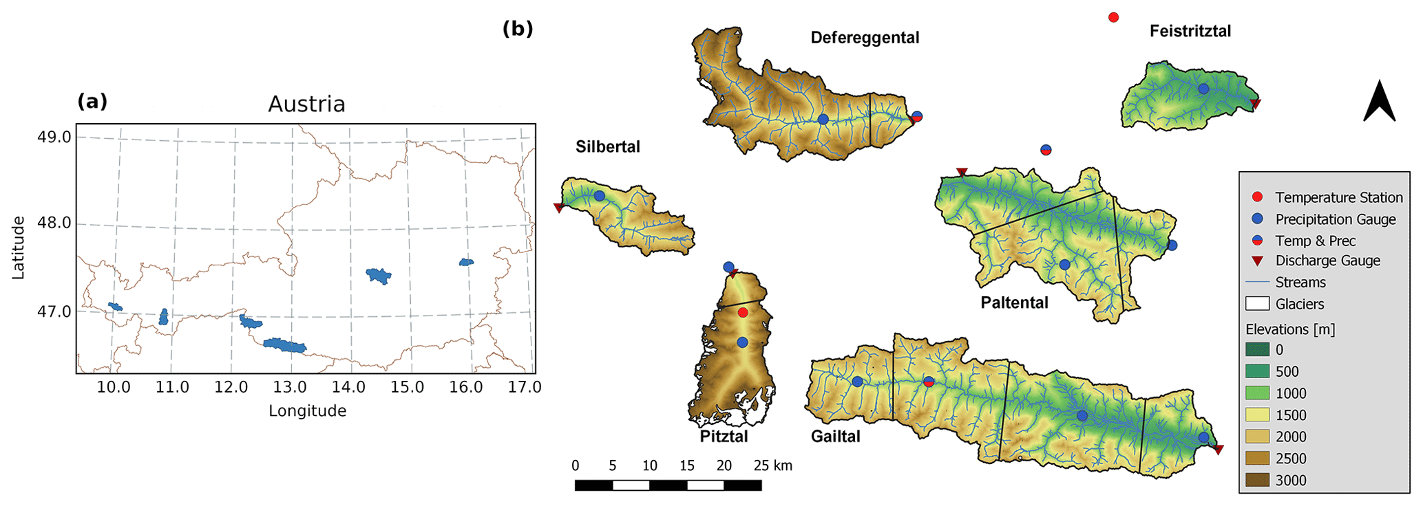
Figure 1 (a) Location of the six study catchments in Austria (shaded blue area). (b) Elevation maps of the study catchments, including the location of precipitation and temperature observation stations, as well as the division into precipitation zones (black lines).

Table 1 Catchment characteristics. Precipitation and temperature are based on data from 1986–2010 used in this study. Runoff coefficients are based on simulations of this study. The runoff regimes are based on Mader et al. (1996).

Daily runoff sums are taken from the Hydrographic Service of Austria (https://ehyd.gv.at/, last access: 15 June 2021; 1985–2015). Temperature and precipitation data are made available from Austrian Central Institute for Meteorology and Geodynamics (ZAMG) and the Hydrographic Service of Austria (1980–2015; Fig. 1). Precipitation data are aggregated and temperature data are averaged to a daily resolution. As shown in Fig. 1, precipitation stations are located in the valleys of the catchments at elevations below the mean catchment elevation. However, in most of the study catchments, the data provide a long-term water balance that is broadly closing and, thus, was assumed to be plausible. Since the long-term precipitation for the Defereggental and Silbertal catchments is lower than long-term runoff, the measured runoff is scaled such that the long-term water balance matches the Budyko framework. Hereby, we decided to scale the runoff data rather than the precipitation data because the precipitation of climate simulations match historical precipitation observations, and this study focuses on changes in runoff rather than absolute values. Using this approach, climate simulations can be left unchanged. Daily potential evaporation is estimated based on daily temperature and potential sunshine hours using the Thornthwaite method (Thornthwaite, 1948; Oudin et al., 2005). The Thornthwaite method compared well with published estimates of potential evaporation in the Austrian Alps (BMLFUW, 2007; Kling, 2006), while the Hargreaves method (Hargreaves and Samani, 1985), another temperature-based method, overestimated potential evaporation.

Land use types of the catchments are determined using the CORINE Land Cover data set from 2018 (https://land.copernicus.eu/pan-european/corine-land-cover, last access: 15 June 2021), and the riparian zone is determined based on a 10×10 m height above nearest drainage (HAND) map (Gharari et al., 2011). Glacier outlines of the past are taken from the Austrian Glacier Inventory (Lambrecht and Kuhn, 2007; Abermann et al., 2010). A linear interpolation between the observation years is applied, and the change in glacial area between 1997 and 2006 is extrapolated to 2015. Zekollari et al. (2019) simulate the future evolution of glaciers in Europe with GloGEMflow, a recent extension of the Global Glacier Evolution Model (Huss and Hock, 2015) that considers ice flow explicitly. Future simulated glacier extents in the Pitztal catchment under different emission scenarios are used in this study. These are scaled to match the extrapolated glacier areas in 2015.

Daily gridded snow cover data for the 2000–2015 period from the MODIS satellite product MOD10A1 (Hall and Riggs, 2016) are used, in addition to the daily runoff data for the calibration of the hydrological model. Moreover, a 10×10 m digital elevation model of Austria (https://www.data.gv.at/katalog/dataset/dgm, last access: 15 June 2021) is used to derive topographic information.

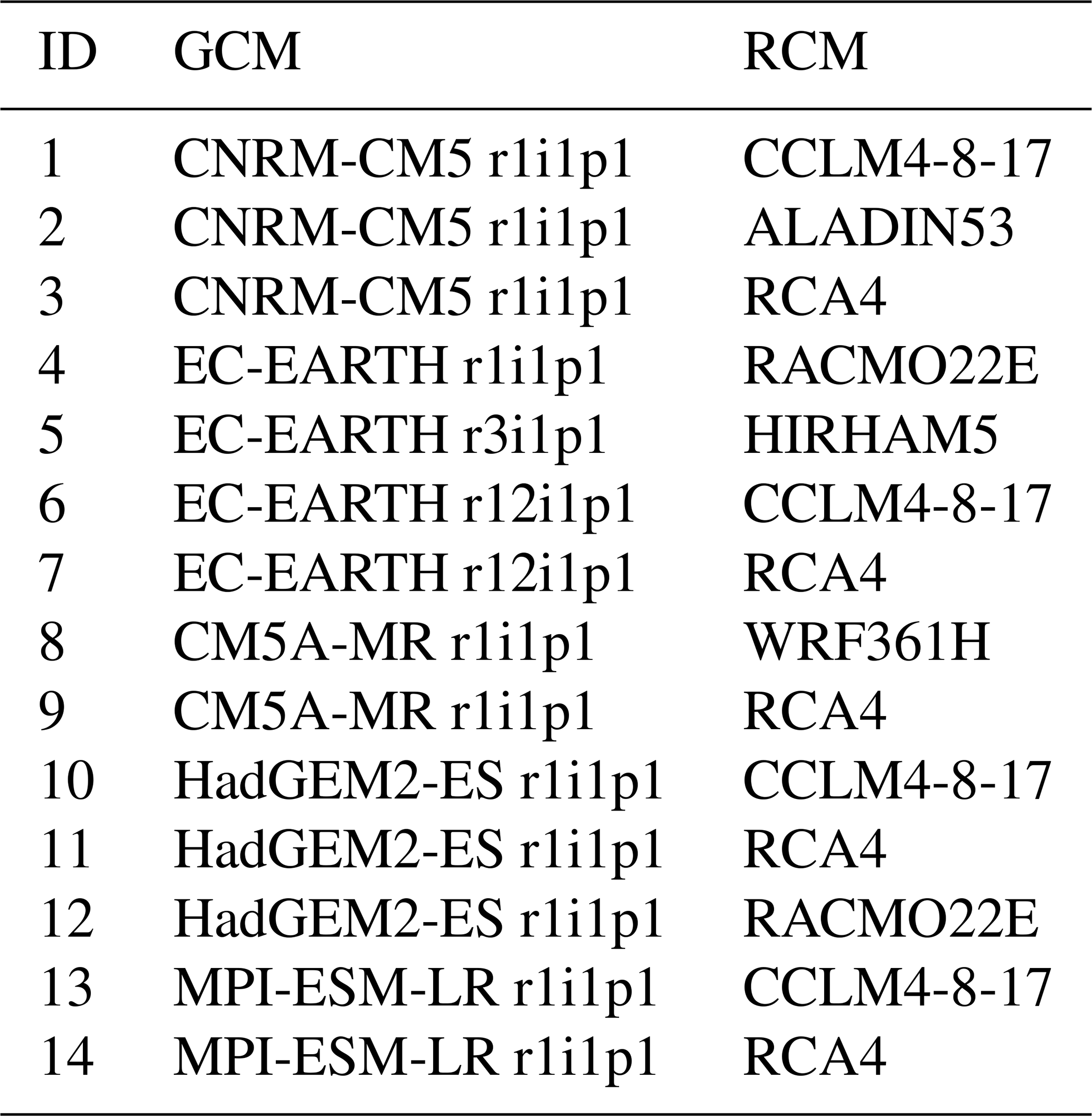
In addition, past and future temperature and precipitation estimates at the station scale are obtained for the 1981–2010 and 2071–2100 periods from 14 high-resolution climate simulations generated based on the EURO-CORDEX data set (Jacob et al., 2014, Table 2) and bias corrected using scaled distribution mapping, with a gamma distribution to remove systematic model errors, for the two emission scenarios RCP4.5 and RCP8.5 (Switanek et al., 2017). RCP4.5 is an intermediate pathway where emissions are partly reduced, yielding 4.5 W m⁻² radiative forcing by the year 2100. RCP8.5 represents a pathway with increasing greenhouse gas emissions and no mitigation measures. The simulations provide the temperature and precipitation data on a daily basis at the station scale corresponding to the location of precipitation and temperature stations (Fig. 1; Switanek et al., 2021).

Table 2 EURO-CORDEX models used for this study (Jacob et al., 2014). The model resolution is 12.5×12.5 km. The rip index refers to realization, initialization method and physics version used for GCMs.

2.2 Hydrological model

2.2.1 Model structure

A semi-distributed, process-based hydrological model is used to model the runoff behavior of the catchments. The model is based on hydrological response units (HRUs), as utilized and described, for example, by Gao et al. (2014) and Prenner et al. (2018). The aim is to represent dominant physical processes in the catchment based on topography and land cover classes while limiting model complexity (Savenije, 2010). A detailed model description is given in Sect. S1 in the Supplement.

Briefly, the following storage reservoirs are included in the model and represented by the water balance equations (Table 3): snow, interception, unsaturated root zone, as well as a fast- and a slow-responding groundwater component. In total, the model is implemented with a hierarchy of three levels of spatial resolution which are, in ascending resolution, (i) one to four precipitation zones per catchment (Fig. 1), (ii) the four HRUs per precipitation zone (Fig. 2) and (iii) individual 200 m elevation zones per HRU (e.g., Roodari et al., 2021).

Table 3 Relevant water balance and constitutive equations of the hydrological model. Reservoirs/states (mm): S_fast – fast-responding reservoir; S_glacier – glacier reservoir; S_int – interception reservoir; S_slow – slow-responding reservoir; S_snow – snow reservoir; S_u – soil reservoir. Fluxes (mm d^-1): E_int – interception evaporation; E_u – evapotranspiration; M_tot – melt; P – precipitation; P_snow – precipitation as snow; P_eff,(tot) – (total) effective precipitation; q_base – base flow; q_fast – fast runoff; q_over – overland flow; q_pref – preferential flow; q_rip – capillary rise riparian zone. Parameters: β (–) – factor accounting for nonlinearity; F_evap (–) – evapotranspiration control factor; F_melt (mm ^∘C⁻¹) – melt factor; I_max (mm) – max. interception capacity; k_fast (d⁻¹) – fast hillslope constant; k_fast,rip (d⁻¹) – fast riparian constant; k_slow (d⁻¹) – slow constant; M_M (^∘C) – smoothness parameter for melt; ρ_p (–) – share preferential flow; ρ_rip (–) – share riparian flow; S_u,max (mm) – max. soil storage capacity; T_thresh (^∘C) – threshold temperature for precipitation partitioning and melt; area_gl – glaciated area. A detailed model description can be found in Sect. S1.

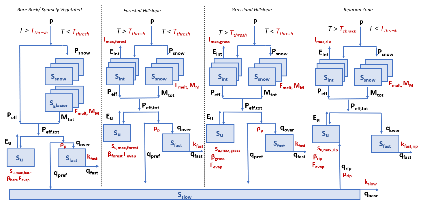
Figure 2 Schematic representation of model structure per precipitation zone, showing model states (blue), fluxes (black) and parameters (red).

More specifically, the division of catchments into precipitation zones is based on available precipitation gauges using Thiessen polygons (Fig. 1). The model is run separately for each precipitation zone with different precipitation input. Catchment-scale model outputs are then obtained for each time step as the area-weighted aggregated outputs of the individual precipitation zones. In each precipitation zone, the model is further discretized into four HRUs (Fig. 2), namely bare rock, forest, grassland and riparian zone. To account for differences in vegetation cover in the individual HRUs, the vegetation-dependent model parameters I_max and S_u,max, representing the water storage capacities in interception and root zone storage reservoirs, were allowed to vary between HRUs. All other parameters are kept constant across HRUs to minimize the number of calibration parameters. Note that interception storage is considered to be negligible in the bare rock HRU. Therefore I_max is set to 0, which removes that storage from the bare rock HRU (Fig. 2). In contrast to the other HRUs, the riparian zone includes the process of upwelling groundwater (q_rip) to sustain soil moisture throughout dry seasons (Prenner et al., 2018; Hulsman et al., 2021). Glaciers are incorporated in the model as an unlimited snow reservoir in the bare rock unit according to their areal extent (Seibert and Vis, 2012; Mostbauer et al., 2018). To allow for elevation-dependent snow dynamics, the HRUs are further stratified into 200 m elevation zones. Snow accumulation and melt in the individual elevation zone is estimated with an improved degree day method, as suggested by Girons Lopez et al. (2020).

2.2.2 Calibration and evaluation

In total, 20 parameters must be calibrated for each catchment, except for the Pitztal, where an additional loss term is implemented to account for artificial diversion of water through a pipe system from the catchment for hydropower generation. All model parameters, including their uniform prior distributions and the ranges of the parameter sets retained as feasible after calibration, are given in Table S1 in the Supplement. The parameter combinations of the individual HRUs are a priori constrained based on relational process constraints as suggested by Gharari et al. (2014) and, similarly, implemented for the study catchments by Prenner et al. (2019, Sect. S2) to ensure process consistency and to limit the effects of equifinality. For a robust representation of model internal dynamics, we further adopt an extended multi-objective and multivariable calibration strategy (e.g., Efstratiadis and Koutsoyiannis, 2010). To do so, we train the model to simultaneously optimize eight objective functions, describing different signatures of flow, and the presence of snow cover (Table 4). Detailed descriptions of the signatures and objective functions are provided in Sect. S3. The overall model performance is assessed by an objective function based on the mean Euclidean distance from the theoretical perfect model (e.g., Hrachowitz et al., 2014; Hulsman et al., 2021): ${\mathrm{Obj}}_{\mathrm{tot}}=\mathrm{1}-\sqrt{\frac{\sum _{n=\mathrm{1}}^N(\mathrm{1}-{\mathrm{Obj}}_n{)}^{\mathrm{2}}}{N}}$, where 1 indicates a perfect model. To ensure balanced solutions, and in the absence of more detailed information, the individual objective functions were equally weighted to compute Obj_tot.

Nash and Sutcliffe (1970)Nash and Sutcliffe (1970)Criss and Winston (2008)Euser et al. (2013)Euser et al. (2013)Hrachowitz et al. (2014)Hrachowitz et al. (2014)Finger et al. (2015)

Table 4 Signatures and the associated objective functions (Obj_n) used for model calibration and post-calibration model evaluation, including the Nash–Sutcliffe efficiency (E_NSE), the volumetric error (E_VE) and the relative and absolute error (E_RE, E_AE).

The models are calibrated using in situ observations of precipitation, temperature and runoff with a Monte Carlo sampling scheme based on 3 million realizations for each catchment. Calibration is run for a period of 20 years (October 1985–October 2005), with a prior warm-up period of 3 years.

After calibration, the models are evaluated using the available flow data after the calibration period (November 2005–2013 or 2015, depending on the catchment). For the post-calibration model evaluation, the same objective functions as for calibration were used. To partially capture the model uncertainty but limit the amount of data for further analysis, the best 0.01 % of the calibrated parameter sets (300 sets), based on Obj_tot during calibration, were used for further analysis, with an additional constraint of Obj_tot>0.8 during calibration. This decision allows an ensemble analysis of plausible solutions, based on the concept of equifinality, suggesting that observed hydrological response dynamics can be reproduced by many different parameter sets (Beven and Binley, 1992).

2.3 Climate simulations as model input

To analyze the effect of a changing climate on the hydrological response, the model was run using climate simulations for a 30-year period in the past (1981–2010) and a period at the end of the 21st century (2071–2100). Although uncertainties are larger at the end of the century than for the mid-century, the stronger climate change signal enhances detection of potential changes due to climate change. The modeled flow characteristics, i.e., the model output, for the two individual 30-year periods were then quantitatively compared. While the climate simulations for the calibration period match the statistical distribution of the hydro-climatic drivers, they do not match their timing. In other words, the simulations of past precipitation and temperature are not concomitant with the in situ observations of flow at the daily timescale of the model application. Therefore, the model had to be calibrated using in situ observations (Sect. 2.2). To use the calibrated model parameters in a meaningful way in combination with the simulations of the past and future, we first test whether the long-term distributions of the in situ data and the modeled climate for the 1981–2010 period are equivalent to avoid misinterpretation of the model results. In addition, we also compare the long-term distributions of modeled flow using both in situ and simulated hydro-meteorological input for the 1981–2010 period to assess the presence of potential systematic errors. After these tests of data equivalence, we generate 300 model simulations using the parameter sets retained as the best (Sect. 2.2) for each of the 14 individual climate simulations (Table 2), for each of the two emission scenarios (RCP4.5 and RCP8.5; Sect, 2.1) and for both the 1981–2010 and the 2071–2100 periods. In total, this results in a total of ∼100 000 individual 30-year daily model realizations. While the glacier extent in the Pitztal catchment is adapted over time, as described in Sect. 2.1, and the glacier extent in the Defereggental catchment is assumed to be negligible for the future period, the other HRUs are kept constant over time.

2.4 Analysis of change

Simulations of past and future runoff are compared for the same climate simulation and parameter set, using averages over the 30-year time period. The methods used to analyze changes in extreme flows are briefly described in the following sections (refer to Sect. S4 for equations).

2.4.1 High flows

To investigate the changes in high flows, an approach similar to Blöschl et al. (2017, 2019) is taken. We generate time series comprising the highest modeled peak flow for each calendar year, i.e., the annual maximum flow (AMF). To analyze the change in magnitudes of high flows, the relative and absolute changes in the mean AMF between the past and the future are quantified for each simulation. In addition, the magnitudes of each year are ranked, and the exceedance probability is calculated. The absolute changes in magnitude for a certain return period, related to an exceedance probability, are calculated per simulation. To compute the mean timing of high flows over the two individual 30-year periods, the method of circular statistics is used (e.g., Young et al., 2000; Blöschl et al., 2017). This method computes time differences between events correctly despite the turns of the year. Nevertheless, a bimodal flood season would be hidden by this approach, as the average date of occurrence would be located between the two seasons. Therefore, additionally, the distribution of timing in the two 30-year periods is analyzed by computing the relative frequencies of AMF occurring within individual 15 d periods. A 15 d period is chosen to allow observations of relatively small change over time while being long enough for multiple events to co-occur in the same period.

2.4.2 Low flows

Changes in low flows are analyzed using the annual minimum average runoff of 7 consecutive days. This minimum average runoff is computed using a moving average from June to May to avoid complications with turns of the year, as low flows are expected mainly in winter (Vormoor et al., 2017; Jenicek et al., 2018). The mean timing over the two individual 30-year periods and the distribution of timing in these periods are computed with the same approach as for high flows, i.e., using circular statistics.

3 Results

3.1 Hydrological model calibration and evaluation

Overall, the models reproduce the main features of the observed hydrological response for both the calibration and the evaluation periods in all study catchments with Obj_tot=0.82–0.89 and 0.80–0.89, respectively (Fig. 3). The model performance with respect to the individual objective functions remains relatively stable between the calibration and evaluation periods with, for example, $E_{\mathrm{NSE},Q}=\mathrm{0.71}$–0.85 only experiencing very minor reductions to 0.69–0.86 (Fig. 3). Closer inspection of the modeled hydrographs indicates that the short-term flow dynamics are generally adequately captured (Figs. 4 and S1–S12 in the Supplement). However, in some cases, peak flows that are in most cases likely to be associated with very localized, high-intensity convective rainfall events, remain underestimated due to uncertainties in precipitation observations (Hrachowitz and Weiler, 2011). In contrast, the modeled mean regime curves of flow over the combined calibration and evaluation periods match the observations rather well (Fig. 5), indicating that the models adequately capture the general magnitudes and seasonal patterns in all study catchments.

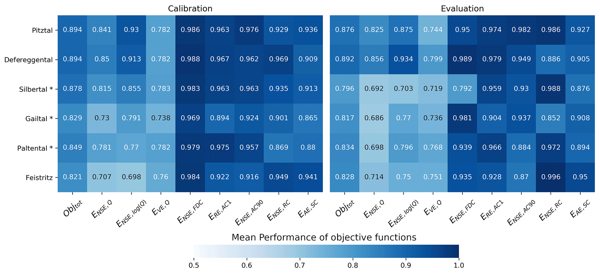
Figure 3 Mean model performance of the best 300 parameter sets for the calibration and evaluation periods. Obj_tot shows the overall model fit. Table 4 gives a description of the objective functions. The asterisk (^*) indicates the catchments that use 8 years of evaluation instead of 10.

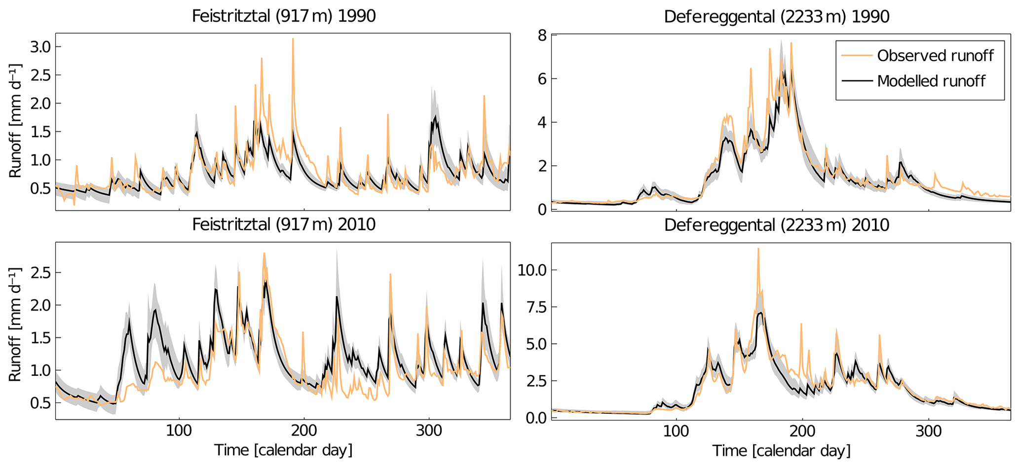
Figure 4 Comparison of measured and modeled runoff for 1 year during the calibration period (1990) and 1 year during the evaluation period (2010). The black line indicates mean modeled runoff using best parameter sets, and the shaded area corresponds to the range of best parameter sets.

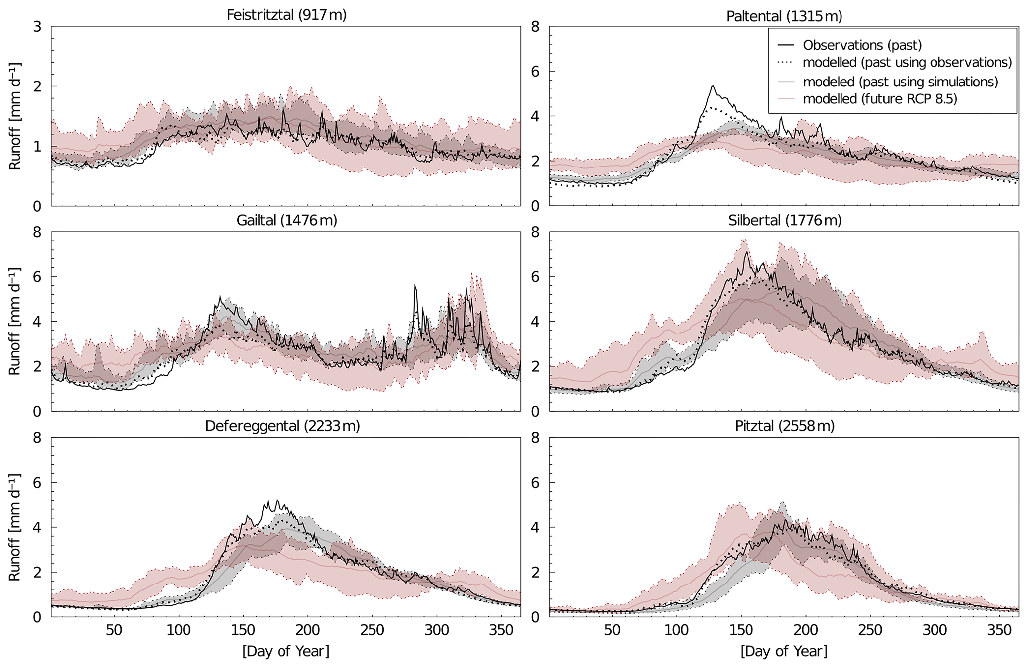
Figure 5 Comparison of observed (black line) and modeled runoff regime in the past (1985–2013), using meteorological observations (dotted line), as well as runoff regimes modeled by climate simulations in the past (1981–2010) and future (2071–2100) for RCP8.5 (gray and red lines represent the mean flow regime within the range of 14 climate models, as shown by the shaded area). Note that the extent of the y axis differs for the Feistritztal catchment.

3.2 Simulation of historical climate and hydrology

The seasonality of precipitation and temperature of climate simulations in the period 1981–2010 closely matches the seasonality of the measured station data. For the high-elevation catchments (Silbertal, Defereggental and Pitztal), the climate models slightly underestimate the monthly temperatures, mostly in the summer months (e.g., Silbertal catchment in Fig. 6 and other catchments in Fig. S13–S17). The difference in mean annual temperature between simulations and observations in the past is much lower (on average 0.5 ^∘C) than the difference in mean annual temperature between past and future simulations. As this study focuses on the projected changes, we expect the results to be valid if the model slightly under- or over-predicts precipitation or temperature in the calibration period. The seasonality in the observed monthly runoff is generally well represented by the modeled runoff using climate simulations. However, monthly observed and modeled runoff show some disagreements. For example, in high-elevation catchments, the monthly runoff, generated using climate simulations, is generally underestimated in spring and early summer, whereas it is overestimated in late summer (Figs. 6 and S16–S17). This is likely to be related to the underestimation of temperature in these catchments in the climate simulations, which delays runoff due to later snowmelt (Fig. 6). Since bias correction was performed over a longer time period (1961–2010) than this comparison (Figs. 6 and S16–S17), and since RCMs do not align in time with observations, any subperiod will invariably somewhat differ from the observed distribution.

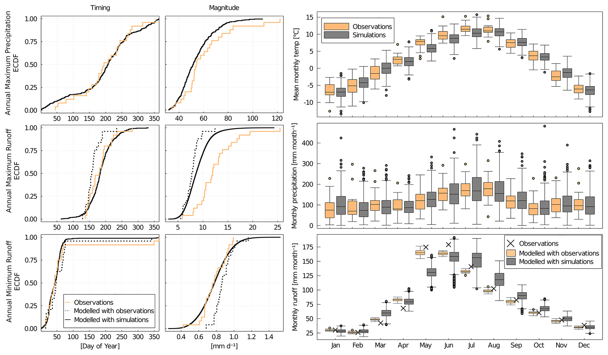
Figure 6 Comparison of past hydro-climatic data and runoff obtained from in situ observations and from climate simulations in the Silbertal catchment. The empirical cumulative distribution functions compare the timing and magnitudes of annual extremes derived from in situ observed data and from all climate models. The box plots compare the distributions of mean monthly temperatures, monthly precipitation and monthly runoff derived from in situ observations and modeled climate. Note that the crosses indicate the actual in situ observations of mean monthly runoff.

While the distributions of the timing of annual extreme events (i.e., the annual maximum precipitation, maximum runoff and minimum runoff) modeled under the simulated climate are broadly consistent with in situ observations, the distributions of the associated magnitudes of these annual extremes exhibit some more disagreement. Although precipitation and minimum modeled runoff magnitudes obtained from in situ observations match those obtained from climate simulations generally well, observed annual maximum runoff is systematically underestimated by model results for all catchments (Figs. 6 and S13–S17). These underestimations are likely associated to an insufficient representation of localized, high-intensity rainfall events. As the main objective of the subsequent analysis is a quantification of the changes between the past and future flow characteristics rather than a prediction of absolute magnitudes, we assume, in the absence of more information, that these systematic errors remain constant over time and should, therefore, not significantly affect the interpretation of the analysis.

3.3 Projection of future climate and hydrology

3.3.1 Annual, seasonal and monthly averages

First, the changes in average projected annual temperature, precipitation and modeled runoff between the 30-year periods in the past and the at the end of the 21st century are analyzed (Fig. 7b). The increase in temperature is similar across catchments, with a median increase across climate simulations of 2–3 ^∘C for RCP4.5 and 4–5 ^∘C for RCP8.5. On average, climate simulations show an increase of annual precipitation by 4 % (RCP8.5; Gailtal) to 9 % (RCP8.5; Defereggental). The median absolute change ranges from 50 to 100 mm yr⁻¹ across catchments. However, the spread between climate simulations is large, reaching from a decrease of 10 % or larger for all catchments to an increase of more than 15 %. Generally, a decrease in precipitation is projected for July and August for most catchments, while an increase in precipitation is projected for the rest of the year (Fig. S19). For RCP4.5, the modeled annual runoff exhibits an increase by around 5% for all catchments except the Pitztal, where a median increase of 12 % was modeled (Fig. 7b). For RCP8.5 the median change is around zero for the lower-elevation catchments of Feistritztal, Paltental and Gailtal, whereas it is slightly larger than for RCP4.5 in the Defereggental and Pitztal catchments. Hence, the change in annual runoff is larger for high-elevation catchments under RCP8.5. However, the spread between simulations is large.

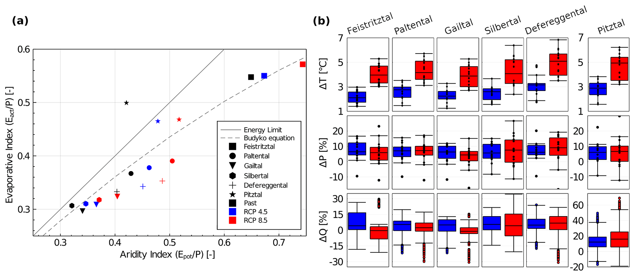
Figure 7 (a) The position of the study catchments in the Budyko framework (Budyko, 1948), based on the 30-year means of all climate simulations in the past and under two emission scenarios at the end of the 21st century. E_act is actual evaporation defined as $\mathrm{1}-\frac{Q}{P}$. (b) Absolute changes between past and future in mean annual temperature, as well as relative changes in mean annual precipitation of the 14 climate simulations (black dots representing the individual climate simulations) and in annual runoff of all simulations for RCP4.5 (blue) and RCP8.5 (red). Note the different scale for the runoff of the Pitztal catchment.

Furthermore, the changes in the catchments in the Budyko framework follow a bottom-left to top-right trajectory, indicating a shift towards considerably more arid future conditions (Fig. 7a). Largely linked to increases in atmospheric water demand, i.e., E_pot, this will lead to proportionally higher future evaporation and associated decreases in runoff coefficients. The change is around twice as large for the RCP8.5 scenarios compared to RCP4.5. Note that, in the past, the Pitztal catchment plots above the energy limit in the Budyko framework using modeled climate, but this is not the case when relying on in situ observed data. The impact on the results should be limited because a relative comparison of past and future runoff patterns is applied using climate simulations for both periods.

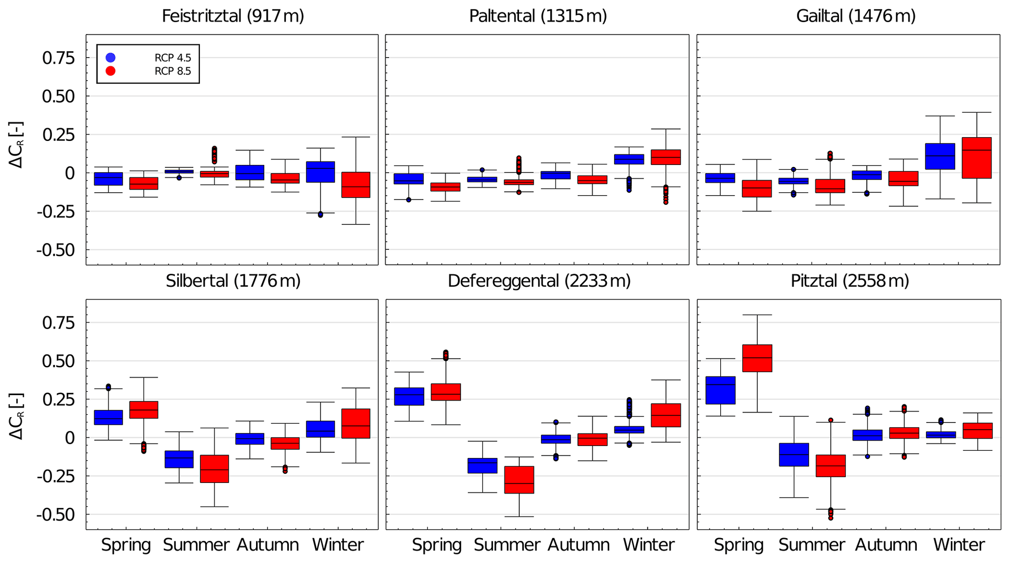
Figure 8 Absolute changes in mean seasonal runoff coefficient (ΔC_R (–)) across all 14 simulations for the six study catchments and both scenarios RCP4.5 and RCP8.5 (spring – March–May; summer – June–August; autumn – September–November; winter – December–February). Mean catchment elevation is given in parentheses.

Analyzing the change in seasonal modeled runoff coefficients, $C_{\mathrm{R}}=Q/P$, similarly reveals substantial differences between the low-elevation and the high-elevation catchments. For the high-elevation catchments, a median future increase in C_R across all 14 simulations is observed in spring (ΔC_R∼0.1–0.5) and, to a lesser extent, in winter (ΔC_R<0.1) (Fig. 8), while the summer runoff coefficients experience considerable decreases by up to $\mathrm{\Delta }{C}_{\mathrm{R}}\sim -\mathrm{0.3}$. In contrast, the lower-elevation catchments are mostly characterized by a decrease in median spring, summer and autumn runoff coefficients of up to $\mathrm{\Delta }{C}_{\mathrm{R}}\sim -\mathrm{0.1}$ but an increase in winter (ΔC_R∼0.05–0.15).

The modeled mean monthly runoff at the end of the century exhibits mostly consistent increases in winter and spring months (ΔQ∼25 %–100 % for RCP4.5) and decreases in summer months (ΔQ∼10 %–20 % for RCP4.5) in all study catchments (Fig. 9). Changes are up to twice as large for RCP8.5 compared to RCP4.5, and the spread between simulations is also larger. The largest relative and absolute increase in runoff occurs considerably later in high-elevation catchments. For the Gailtal catchment, the largest absolute increase occurs in February (ΔQ∼0.6–0.8 mm d⁻¹), while for the Silbertal (ΔQ∼0.8–1.2 mm d⁻¹) and Defereggental catchments (ΔQ∼0.8–1.0 mm d⁻¹) this is the case in April and for the Pitztal catchment in May (ΔQ∼1–1.4 mm d⁻¹). The two lowest elevation catchments, i.e., Feistritztal and Paltental, do not show a distinct month with the largest increase in runoff. Decreases in monthly runoff can already be expected in May for the three low-elevation catchments, whereas this only occurs from June or July onwards in the high-elevation catchments (Fig. 9). The results also indicate that the magnitude of absolute change in monthly runoff generally increases with increasing mean catchment elevation. While the change is very limited for the Feistritztal catchment (ΔQ±0.2 mm d⁻¹), it is more pronounced in the Gailtal catchment (ΔQ±0.9 mm d⁻¹), reaching the strongest decrease and increase in the Silbertal catchment ($\mathrm{\Delta }Q\sim -\mathrm{1.5}$ mm d⁻¹) and Pitztal catchments (ΔQ∼1.5 mm d⁻¹), respectively.

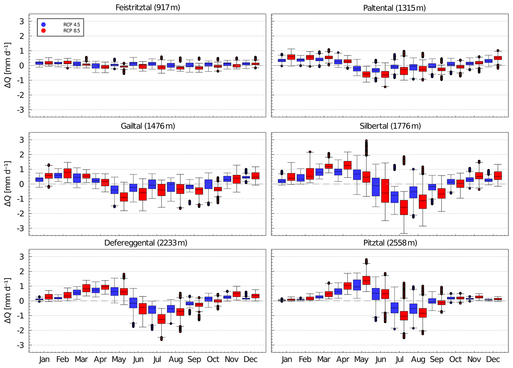
Figure 9 Absolute changes in future mean monthly runoff (ΔQ) across all simulations per RCP for the six study catchments. Mean catchment elevation is given in parentheses.

A decrease in future annual melt contribution is projected in all study catchments, ranging from $\mathrm{\Delta }M\sim -\mathrm{10}$ % to −30 % for RCP4.5 and $\mathrm{\Delta }M\sim -\mathrm{20}$ % to −55 % for RCP8.5. The results do not show the direct contribution of meltwater to runoff but the contribution of meltwater to the hydrological storages and processes that eventually generate runoff. The amount of meltwater in the low-elevation Feistritztal catchment is small compared to all other catchments (Fig. 10). For the high-elevation catchments, an earlier future onset of melt can be detected with the largest increase of ΔM∼25 mm per month for the Silbertal and Defereggental catchments in March and ΔM∼35 mm per month for the Pitztal in May. In addition, a remarkable decrease in melt from June through September is observed for the high-elevation catchments. Generally, the month with the largest melt rates shifts to 1 month earlier in the year. Differences between the two emission scenarios are mostly visible in lower melt rates from May to July in most catchments for RCP8.5. As opposed to the high-elevation catchments, no substantial increase in snowmelt in the first months of the year is observed for the lower catchments.

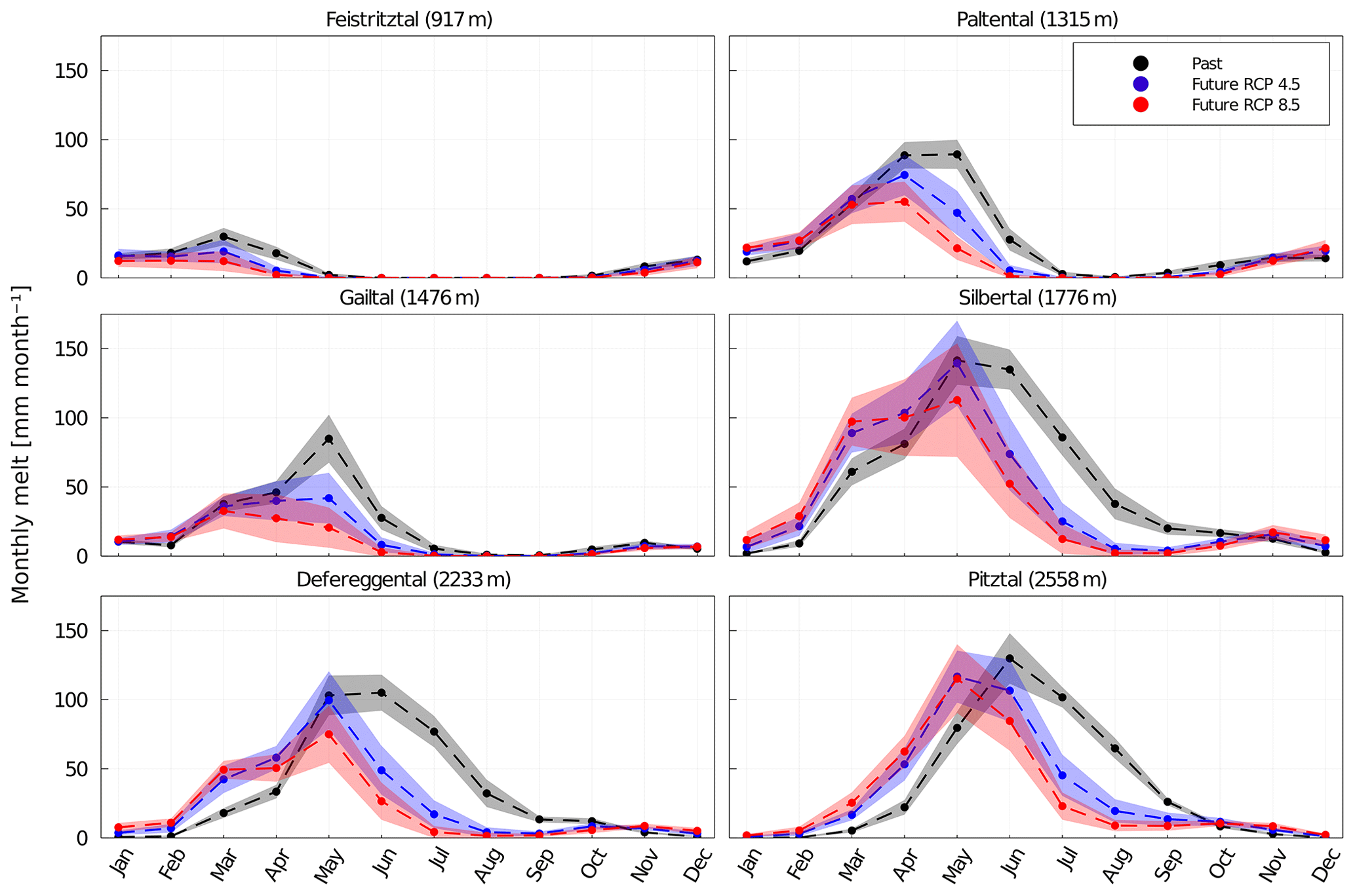
Figure 10 Mean monthly melt contributions in the past (black dots) and future (blue dots – RCP4.5; red dots – RCP8.5) over the time period of 30 years. The shaded areas indicate the associated ±1 SD (standard deviation; gray – past; blue – RCP4.5; red – RCP8.5). Dashed lines between the individual months are used for better visualization.

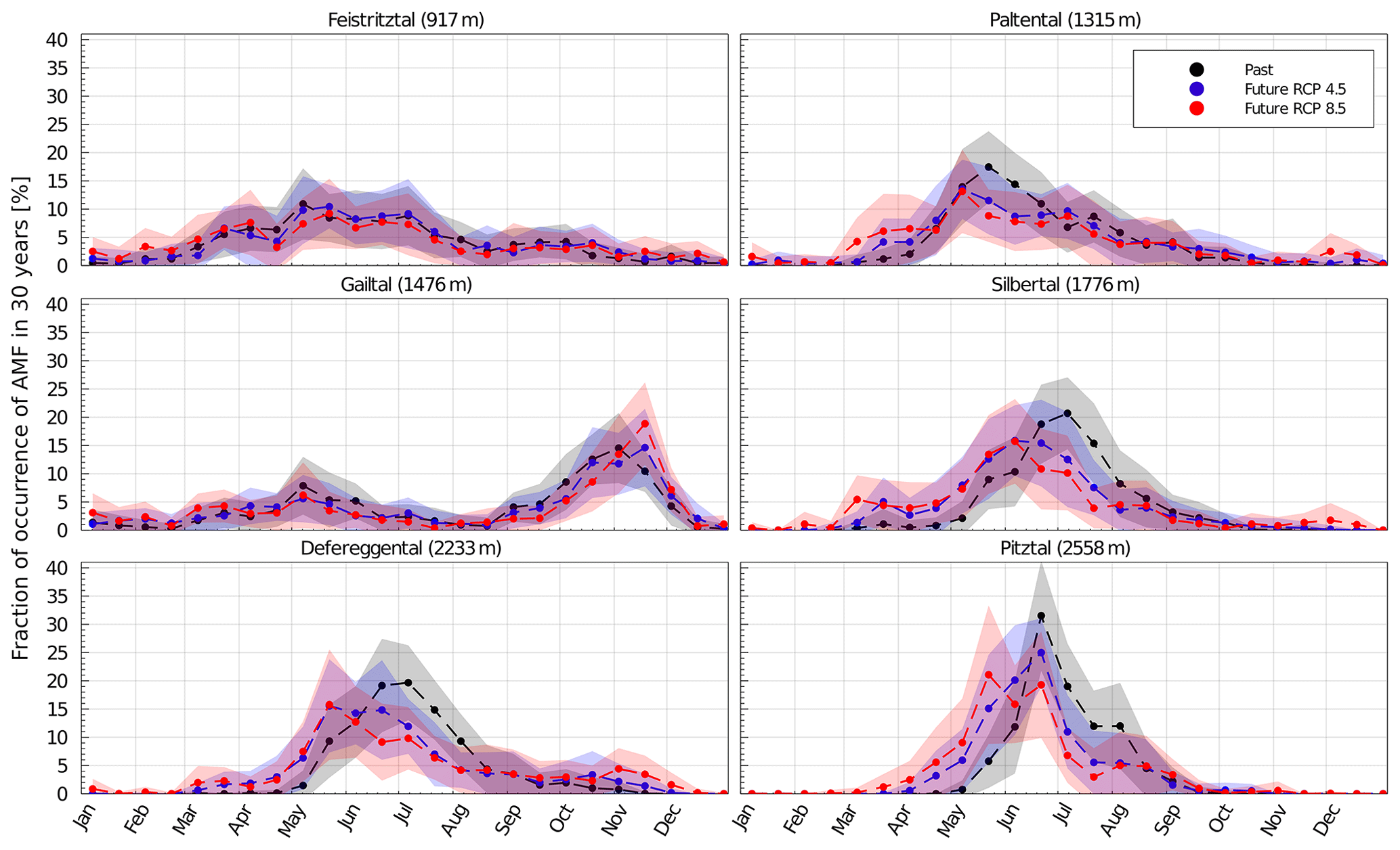
Figure 11 Mean fraction of occurrences of AMF in the past (black dots) and future (blue dots – RCP4.5; red dots – RCP8.5) for 30-year time periods, using time windows of 15 d across all model simulations. The shaded areas indicate the associated ±1 SD. Dashed lines between the individual 15 d periods are used for better visualization.

Table 5 Mean and standard deviation of timing of annual maximum flow (AMF) across all simulations, based on the average timing of AMF over 30 years of each simulation. The dates are shown as the day of the year. For the past, the actual calendar date is given as a reference.

3.3.2 Annual maxima (timing and magnitude)

A substantial shift in the timing of annual maximum flows (AMFs) is observed towards the end of the 21st century, ranging, on average, from $\mathrm{\Delta }t=-\mathrm{9}$ to −31 d for high-elevation catchments and $\mathrm{\Delta }t=+\mathrm{4}$ to −17 d for low-elevation catchments (Table 5). More specifically, in the past, AMF occurred, on average, in the first week of July in the high-elevation catchments and around 1 month earlier in two of the low-elevation catchments (Feistritztal and Paltental). In the Gailtal catchment, AMF occurred, on average, in the first week of October. AMF in the higher catchments is characterized by a $\mathrm{\Delta }t=-\mathrm{11}$ to −20 d on average for RCP4.5, with the Silbertal catchment exhibiting the largest shift of $\mathrm{\Delta }t=-\mathrm{20}$ d. For RCP8.5, the Defereggental catchment shows a similar shift as for RCP4.5, whereas the Silbertal and Pitztal catchments show an increased Δt of −31 and −22 d. The lowest catchments only exhibit a minor change in the mean timing of AMF for RCP4.5 and an average shift towards occurrences 2 weeks earlier for RCP8.5. The Gailtal is the only catchment exhibiting a systematic and substantial shift towards later occurrences of AMF with a modeled mean $\mathrm{\Delta }t=+\mathrm{29}$ d for RCP4.5 and +48 d for RCP8.5. In addition, for all catchments except the Gailtal, the future standard deviation of the AMF timing increases (Table 5). However, mean timing may conceal bimodal distributions in the timing of AMF. Analyzing the fraction of the timing of occurrence within the individual 30-year time periods gives additional information about the intensity of seasonality (Fig. 11).

Figure 12 (a) Violin plots of the relative change in magnitude of AMF across simulations, based on average magnitude over 30-year time period of each simulation. (b) Simulation mean absolute change in magnitudes of AMF in relation to the return period. Shaded area indicates 1 SD, and dotted lines are used for better visualization. Note the different scale for the Gailtal catchment.

This analysis reveals a bimodal AMF distribution in the Gailtal catchment, with AMF potentially occurring in beginning of May or beginning of October. A relationship between the mean elevation of the catchment and timing and seasonality of AMF can be observed for the past. For the lowest elevation catchment (Feistritztal), AMF occurrences are widely spread over the year, with most occurrences around the beginning of May. The Paltental catchment shows most occurrences towards end of May, whereas the high-elevation catchments exhibit most AMFs in June and July and feature the highest seasonality. A systematic and significant shift towards earlier occurrences of annual maximum flows can be distinguished for the higher-elevation catchments. However, the model results suggest that the Paltental catchment may also experience a substantial future increase in AMF occurrences in March for RCP8.5. Across all study catchments, except the Gailtal catchment, the seasonality in the timing of AMF is less pronounced in the future. An extension of the potential future flood season by 1 to 3 months can be derived from visual inspection of Fig. 11. Changes are more pronounced for RCP8.5, with a larger spread of timing of AMF over the year.

The change in modeled median average magnitude of AMF over 30-years (ΔAMF) is positive for all catchments under RCP4.5 by ∼10 %. The Paltental and Pitztal catchments show somewhat lower (ΔAMF∼2 %) and higher increases (ΔAMF∼18 %), respectively (Fig. 12a). The absolute changes are largest for the Gailtal (ΔAMF∼1.4 mm d⁻¹) and the Pitztal (ΔAMF∼1.1 mm d⁻¹) catchments. The ΔAMF is less pronounced in most catchments for RCP8.5, even suggesting potential decreases in future AMF magnitudes in the Paltental catchment. However, the ranges of change and, thus, the uncertainties are large, in particular for the Paltental, Silbertal and Defereggental catchments, where simulations also indicate the possibility of a decrease in future AMF magnitudes. A larger absolute increase in magnitude of AMF for higher return periods is simulated, as is the increasing uncertainty (Fig. 12b). The standard deviation of an ΔAMF associated with a return period of 1 year is 0.5 to 2 mm d⁻¹, whereas it reaches 1.7–9 mm d⁻¹ for an ΔAMF associated with a return period of 30 years. A similar pattern can be observed for relative changes. The largest increase in magnitude of AMF at high return periods is found for the Gailtal for RCP8.5 with ΔAMF∼8 mm d⁻¹ (+40 %), followed by the Pitztal with ΔAMF∼3 mm d⁻¹ (+32 %) for both emission scenarios. The two lowest elevation catchments, Feistritztal and Paltental, only show smaller increases of ΔAMF∼0.6 and 1.0 mm d⁻¹, respectively. For shorter return periods, the changes in AMF are less pronounced and consistent across all catchments.

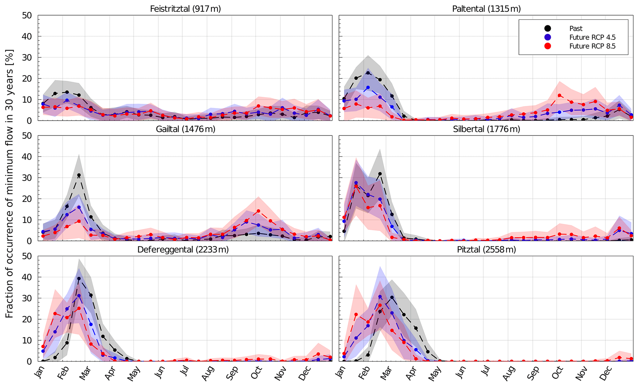
Figure 13 Mean fraction of occurrences of lowest annual 7 d flow in the past (black dots) and future (blue dots – RCP4.5; red dots – RCP8.5) 30-year time periods, using time windows of 15 d across all model simulations. The shaded areas indicate the associated ±1 SD. Dashed lines between the individual 15 d periods are used for better visualization.

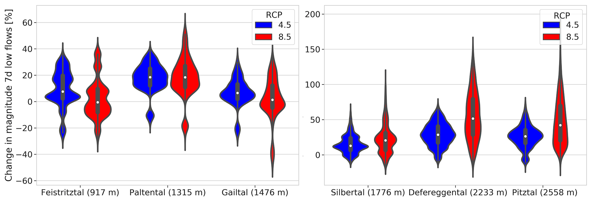
Figure 14 The relative change in magnitude of annual minimum 7 d flows for the late 21st century (2071–2100 vs. 1981–2010). Note the different scales for low- and high-elevation catchments.

3.3.3 Annual minima (timing and magnitude)

In line with observations, the modeled annual minimum flows in the past occurred mostly during the winter months in all study catchments. The model results suggest that, for the low-elevation catchments, the fraction of occurrence of the minimum flows in winter months decreases significantly in the future (Fig. 13). In particular, for RCP8.5, the annual minimum flows shift towards early autumn, with around 13 % of annual minimum flows occurring in late September in the Paltental and Gailtal catchments. In the lower-lying Feistritztal catchment, no clear seasonality in occurrence of minimum flows is distinguishable by the end of the century. In the high-elevation catchments, past annual minimum flows occurred predominantly between late February to March. According to the model results, future annual minimum flows will occur earlier in the year, between January and February.

The magnitudes of the annual minimum flows show a remarkable potential median increase of 12 %–50 % in the high-elevation catchments, with significantly larger increases for RCP8.5 (Fig. 14). The high-elevation catchment of Defereggental shows the largest relative change, with a median increase of $\mathrm{30}\mathit{\%}/\mathrm{50}\mathit{\%}$ for RCP$\mathrm{4.5}/\mathrm{8.5}$, while the second-largest increase is simulated in the highest elevation catchment of Pitztal, with a median increase of $\mathrm{27}\mathit{\%}/\mathrm{40}\mathit{\%}$ for RCP$\mathrm{4.5}/\mathrm{8.5}$. Regarding the low-elevation catchments, the Paltental shows an increase in magnitude of minimum flows of 20 % for both emission scenarios. The median increase in magnitude for the Feistritztal and Gailtal catchments is below 10 % for RCP4.5 and around zero for RCP8.5. While the Defereggental and Pitztal catchments may experience the largest relative median increases of up to $\mathrm{30}\mathit{\%}/\mathrm{50}\mathit{\%}$ for RCP$\mathrm{4.5}/\mathrm{8.5}$, the annual minimum flows will be affected less in low-elevation catchments with median increases of up to around 20 % for both emission scenarios. The absolute changes are largest for Paltental (+0.7 mm d⁻¹), followed by Defereggental under RCP8.5 (+0.47 mm d⁻¹) and Gailtal catchments under RCP4.5 (+0.35 mm d⁻¹). However, from the distributions around the medians (Fig. 14), it can also be seen that, while increases in minimum flow are rather likely for the higher-elevation catchments, the direction of change is subject to much more uncertainty in the lower-elevation catchments.

4 Discussion

4.1 Changes in annual and seasonal climate and hydrology

For temperatures, the sign and magnitude of change are more consistent over all climate simulations than for precipitation. This corroborates the findings of previous climate impact studies in the region (e.g., Goler et al., 2016; Hanzer et al., 2018). The increase in projected future precipitation in Austria is in contrast to results of previous studies that are not based on the EURO-CORDEX ensembles, which suggested no change or a decrease in precipitation (Stanzel and Nachtnebel, 2010; Goler et al., 2016). However, our findings are consistent with the results of an analysis of the EURO-CORDEX ensemble for the Alpine region, as reported by Smiatek et al. (2016). In addition, the modeled increase in annual runoff for the late 21st century (Fig. 6b) is not in line with results from other alpine catchments, which indicate no change or even a decrease in annual runoff (Goler et al., 2016; Muelchi et al., 2020). The median increase in annual runoff of around 5 % for the study catchments under RCP4.5 can be largely explained by the projected future precipitation increase of around 6 %. Under RCP8.5, the low-elevation catchments show a median change in annual runoff of $\mathrm{\Delta }Q\sim -\mathrm{1.5}$ % to 2 %, which is much lower than the precipitation increase of ΔP∼4.5 %–7 %. This slightly lower annual runoff can be attributed to changes in the future partitioning of water fluxes and, thus, an increased fraction of precipitation to be evaporated due to increased atmospheric demand (see Fig. 7a). Increasing atmospheric demand has also been identified as the main driver for increasing evaporation in Austria in the past (Duethmann and Blöschl, 2018). This general decrease in mean runoff coefficients in a warmer climate strongly supports earlier studies (e.g., Berghuijs et al., 2014). The results further strongly suggest that changes in seasonal runoff coefficients and melt contributions are related (Figs. 8 and 10). In seasons with decreasing future melt contributions (i.e., spring or summer for low- or high-elevation catchments), the runoff coefficient decreases, whereas it increases in spring for high-elevation catchments where melt contributions increase in the future. This implies that changes in snow contributions are more important for changes in seasonal runoff than changes in precipitation, as precipitation is projected to increase in future winter and spring seasons. The decrease in summer and autumn runoff coefficients can be explained by decreased precipitation and increased evaporation, which is evident in low-elevation catchments by an increased number of minimum flow events in autumn (Fig. 13). The increase in annual runoff in the future may have a positive impact on hydropower generation. Nevertheless, seasonal changes can lead to decreased energy production in summer and autumn and increased energy production in winter and spring. Management schemes of hydropower production may need to be adapted to such changing seasonal water availabilities, which could potentially be realized by storing seasonal meltwater in artificial basins (Farinotti et al., 2019). Adaptation measures are likely to be higher for RCP8.5 due to larger seasonal changes.

Simulations were performed by changing all variables simultaneously. The attribution of changes to single variables in the discussion is therefore based on expert interpretations of the results and mean changes in monthly precipitation, temperature, snowmelt and potential evaporation (Figs. 10 and S19–S21).

4.2 Changes in monthly runoff

The modeled changes in monthly runoff correspond well with the results of previous studies in the region (Stanzel and Nachtnebel, 2010; Laghari et al., 2012; Tecklenburg et al., 2012), which also report an increase in winter and spring runoff and a decrease in summer runoff. The largest increase in winter runoff occurs later in the season for the high-elevation catchments, which supports findings by Stanzel and Nachtnebel (2010). An explanation gives the later onset of the melting season by 1 month or more in high-elevation catchments (Fig. 10), resulting in increased runoff in later months compared to the low-elevation catchments. Hanzer et al. (2018) simulated changes in monthly runoff in the upper part of the Pitztal catchment and found the largest increases in March, of around 80 % (150 %) for RCP4.5 (RCP8.5), and the largest decreases in August, of around 50 %, which is close to results of this study, with increases of around 100 % to 180 % in March and decreases in August of 20 % to 40 % (Fig. 9).

The increases in future winter runoff can be related to an increase in precipitation (December to February), while increases in melt contribution are largely responsible for the increase in future spring runoff (March to May). In the first 2 months of the year, with negative changes in monthly runoff, the decrease of $\mathrm{\Delta }Q=-\mathrm{5}$ to −24 mm per month can be attributed to a decrease in melt contribution ($\mathrm{\Delta }M=-\mathrm{18}$ to −56 mm per month) in combination with increased potential evaporation (ΔE_pot=5–12 mm per month). Conversely, future precipitation still increases in these months (ΔP=1–24 mm per month). However, the future decreases in runoff during late summer in the low-elevation catchments ($\mathrm{\Delta }Q=-\mathrm{3}$ to −5 mm per month) are mainly a consequence of decreased summer precipitation ($\mathrm{\Delta }P=-\mathrm{4}$ to −8 mm per month) in combination with increased potential evaporation (ΔE_pot=7–9 mm per month) as melt contributions become negligible.

The higher importance of melt contribution for summer runoff in high-elevation catchments compared to the low-elevation catchments can also explain the larger decrease in summer runoff of $\mathrm{\Delta }Q=-\mathrm{14}$ to −24 mm per month compared to $\mathrm{\Delta }Q=-\mathrm{6}$ to 13 mm per month in the low-elevation catchments. Furthermore, a decrease in melt contribution from glaciated areas could potentially be of importance for the decrease in summer runoff in the Pitztal catchment (Hanzer et al., 2018; Laurent et al., 2020). Overall, the decrease in melt contribution and increase in potential evaporation influence the change in monthly runoff more than the changing precipitation patterns, as the maximum decrease in monthly runoff occurs earlier than for monthly precipitation.

The decrease in summer runoff under RCP8.5 is more pronounced than for RCP4.5. This can be explained by a stronger decrease in melt contribution, an increased evaporation and a mostly stronger decrease in monthly precipitation under RCP8.5. The winter and spring runoff under RCP8.5 show an additional increase of ΔQ=2 to 14 mm per month compared to RCP4.5, resulting from a larger increase in snowmelt (Fig. 10). This increased snowmelt directly relates to higher temperatures and a larger average increase in precipitation in winter months under RCP8.5. The Feistritztal catchment is the only catchment with a similar modeled median increase in winter runoff for both emission scenarios. A possible explanation is that the larger decrease in snow contribution is balanced by the higher precipitation under RCP8.5, resulting in a similar change in runoff under both emission scenarios. The changes in monthly runoff could lead to a mismatch between water supply and water demand as mountain regions of the Alps are classified as supportive for the lowlands (Viviroli et al., 2007). However, the Alps are identified as basins where present water demands can also be met in 2060 (Mankin et al., 2017). Therefore, water scarcity due to changes in runoff dynamics in the Alps seems unlikely (Immerzeel et al., 2020).

4.3 Annual maxima (timing and magnitude)

The mean timing of AMF in October for the Gailtal, and June and July for the other catchments, in the past supports the findings of previous studies (Parajka et al., 2009; Blöschl et al., 2011). The high-elevation catchments show a high flood seasonality in the past, suggesting snowmelt as a dominant flood-generating process. For the future, earlier snowmelt is then likely to result in significant shifts in the timing of AMF towards earlier occurrences ($\mathrm{\Delta }t\sim -\mathrm{9}$ to −31 d). For the late 21st century, AMFs occur mostly in May and at the beginning of June, compared to mid-June to early July in the past, which corresponds well with the expected future shift in timing of maximum monthly melt contributions from June to May. Parajka et al. (2010) identified snowmelt and rainfall as an important flood-generating mechanism in the central Alps. A change in the flood-generating processes from snowmelt to precipitation in mountainous catchments and, thus, a shift in the flood season towards the season with highest precipitation was observed in other studies by Vormoor et al. (2015) and Brunner et al. (2020). Thus, changes in precipitation patterns are also likely to contribute to the change in the timing of AMF, as June and July were the months with highest precipitation in past but future precipitation increases are most pronounced in June.

The autumn nival flow regime of the Gailtal catchment is characterized by maximum flows in late spring due to snowmelt and a secondary maximum of flow in autumn due to intensive precipitation (Mader et al., 1996), which translates into high flows occurring both in late spring and autumn (Blöschl et al., 2011). The significant future shift towards later occurrences in AMF in the Gailtal, on the one hand, can be mostly attributed to changes in precipitation patterns, with a larger increase in precipitation in November as compared to October (particularly under RCP8.5), as the timing of floods in southern Austria is strongly influenced by meridional southeasterly and southerly weather regimes (Parajka et al., 2010). On the other hand, earlier annual maximum flows are generated during the first half of the year related to the combination of earlier snowmelt and increased spring precipitation. The average shift of half a month towards earlier occurrences of AMF in the low-lying Feistritztal and Paltental catchments for RCP8.5 is likely related to a more pronounced decrease in AMF occurrences in the summer months. The latter is linked to increased evaporation, and a larger increase in occurrences in spring and winter compared to RCP4.5, connected to increased winter precipitation.

The shift towards later AMF occurrences in the Gailtal catchment and earlier AMF occurrences in the other catchments supports projections for Alpine regions in Switzerland, although no shift in AMF seasonality of highly glaciated catchments was projected there (Muelchi et al., 2021). The seasonality of AMF decreases in the future, and the potential flood season expands by up to 3 months, which is also suggested by Dobler et al. (2012), Köplin et al. (2014) and Schneeberger et al. (2015). This leads to less predictability in the timing of future flood events. The extension of the flood season indicates that future AMF is not only generated by snowmelt or the combination of snowmelt and precipitation but more often only by precipitation. In summary, the timing of AMF in high-elevation catchments with nival flow regimes will continue to depend largely on snowmelt. This emphasizes the importance of temperature change for runoff patterns in alpine catchments. In contrast, in the low-elevation catchments, where a seasonality in the timing of AMF is less pronounced today, future shifts occur mostly due to changes in precipitation patterns and increased evaporation.

The mean increase in the magnitude of AMF for all catchments, except for the Paltental for RCP4.5, is in contrast to findings by Holzmann et al. (2010) who reported a future decrease in AMF magnitudes for mesoscale catchments in western Austria. Similarly, the results of Thober et al. (2018) suggest a decrease in the maximum runoff for the Alps under future climate conditions. However, for Swiss catchments a future increase in AMF magnitude was projected by Köplin et al. (2014), whereas results of Muelchi et al. (2021) indicate a slight decrease in AMF magnitudes in Swiss catchments, and Brunner et al. (2019a) expect a future decrease or no change in maximum runoff under extreme flow regimes in melt-dominated areas in Switzerland. In this study, a similar relative mean modeled AMF increase in all catchments was modeled for RCP4.5(ΔQ∼10 %), suggesting increased precipitation as the underlying reason, since monthly precipitation increases for all catchments during the main flood season (6 % to 15 %) and precipitation intensity rises by 5 % to 18 %. As the dominant generating mechanism shifts from snowmelt towards rain, increases in AMF magnitudes are possible because they are no longer limited by the amount of snow storage available for melt (Merz and Blöschl, 2003). This is also supported by findings of Schneeberger et al. (2015) for the Lech catchment in Austria, where an increase in temperature without changes in precipitation only leads to minor shifts in flood intensities. The low median increase in AMF magnitude in the Paltental catchment of ΔQ∼2 % under RCP4.5 with large uncertainties is largely the consequence of the strong decrease in snowmelt contribution in May and June, which offsets increases in precipitation and maximum precipitation intensity.

Interestingly, the increase in mean AMF magnitude is lower for four out of six catchments under RCP8.5 compared to RCP4.5. This indicates that not all changes in runoff patterns are more pronounced for the higher emission scenario. In the lowest elevation catchments, Feistritztal and Paltental, increased precipitation is offset by a >50 % larger increase in potential evaporation under RCP8.5. This results in larger dry season soil storage deficits, which buffer precipitation and, thereby, moderate annual maximum flows. For the high-elevation catchments, Defereggental and Silbertal, snow contribution is important in the generation of annual maximum flows. Under RCP8.5, the largest monthly melt contribution, which occurs in May, is lower than under RCP4.5, for which monthly melt contribution was similar for the late 21st century compared to today (see Fig. 10). This decrease in melt contribution, together with higher potential evaporation, is more important for change in AMF magnitudes than the increase in precipitation intensities of 14 %–20 % for RCP8.5 compared to 5 %–16 % for RCP4.5. In the Pitztal catchment, the maximum monthly melt contribution remains similar under both emission scenarios, which can be an explanation for the similar increase in AMF magnitude. In the Gailtal catchment, the increase in AMF magnitudes is higher under RCP8.5. A possible explanation is that, particularly under RCP8.5, changes in precipitation intensities or maximum daily precipitation may be higher for the meridional weather regimes than in the northern Alps and, thus, impact the Gailtal catchment, where rainfall is the main flood-generating mechanism. Overall, the changes induced by increased temperature have a larger effect on the changes in AMF magnitudes under RCP8.5 than changes in precipitation. The latter, however, remain the dominant control on AMF magnitude increases under RCP4.5.

The increase in AMF magnitude is larger for high return periods, especially under RCP8.5. This is a likely consequence of the higher increase in extreme precipitation intensities compared to mean precipitation intensities. However, the uncertainty in AMF magnitudes at higher return periods also increases. The increase in runoff for a 30-year return period modeled in this study is much larger (∼40 % for RCP8.5) than the increase in runoff for a 100-year return period (HQ100) of 4 % for the Gailtal for the middle of the 21st century suggested by Blöschl et al. (2011). For catchments in the region of Silbertal, Defereggental and Pitztal, the study by Blöschl et al. (2011) suggests a decrease in HQ100, which contrasts with our model results. For this comparison, it should be noted that a large uncertainty surrounds runoff magnitudes of high return periods (Fig. 12). One reason for the pronounced uncertainties relates to the evaluation of extreme events, which strongly depends on the chosen time period. Other studies conclude that the natural variability in magnitude of high flows exceeds the change due to climate change, which particularly increases uncertainty for high return periods (Blöschl et al., 2011; Dobler et al., 2012). The increase in the magnitudes of maximum flows may locally entail the need to carefully review flood risk assessments and safety of hydraulic structures designed for lower flood estimates.

4.4 Annual minima (timing and magnitude)

In the higher alpine catchments, the modeled shift towards earlier occurrences of low flows to January and February can be explained by an increase in melt contributions in February to April that translate into an increase in monthly runoff. The minimum flows occur before melting starts. In the low-elevation catchments, the shift in the timing of minimum flows from winter to autumn is mostly linked to an increased potential evaporation (particularly pronounced in July) as well as mostly decreasing monthly precipitation in July to September. Thus, an increased storage deficit in the unsaturated zone in late summer due to increased evaporation leads to longer storage of precipitation before it is released as runoff. This is also reflected by decreased seasonal runoff coefficients in summer and autumn (Fig. 8). The reduction in the monthly water deficit in winter and an increase in late summer projected in this study is in line with findings for other Austrian catchments by Goler et al. (2016), who predict a reduction in days below the Q₉₅ threshold in winter but an increase in summer. Projections of minimum flows in Switzerland indicate timing predominately between August and October (Muelchi et al., 2021), whereas our results indicate future occurrences of minimum annual flows, both in winter and autumn.

The magnitude of the annual minimum runoff mostly increases in high-elevation catchments by ΔQ∼12 %–50 %, which can be related to higher winter precipitation and a decreased amount of water stored as snow (Laaha et al., 2016; Parajka et al., 2016; Marx et al., 2018; Brunner et al., 2019a; Muelchi et al., 2021). Whereas projections for lower catchments in Switzerland show an apparent future decrease in magnitude of minimum annual flows for RCP8.5 (Muelchi et al., 2021), our projections show uncertainty in the sign of change.

4.5 Climate model uncertainty

The results of individual GCM/RCM combinations per RCP were compared to investigate whether a specific GCM/RCM combination (Table 2) corresponds to large systematic changes in the hydrological response across all study catchments. Generally, no single GCM/RCM combination was found to lead to the largest or lowest changes across catchments or across emission scenarios. However, there are substantial differences in modeled changes between GCM/RCM combinations. The GCM/RCM combination with the largest decrease/increase in precipitation yielded the largest/smallest decreases in monthly runoff in summer and early autumn. For changes in runoff in other months, no relationship between the most extreme changes and a given GCM/RCM combination was found. The GCM/RCM combination with strongest decrease in annual precipitation (HadGEM2-ES r1i1p1/CCLM4-8-17) generally produces the smallest magnitudes of annual minimum and maximum flows in the future, whereas the GCM/RCM combinations with largest increase in annual precipitation mostly result in the largest increases in magnitudes of annual minimum and maximum flows. Regarding the timing of AMF, the smallest/largest shift towards earlier occurrences is found for the GCM/RCM combinations, with the largest increase in precipitation/temperature under RCP8.5. The relationship between GCM/RCM combination and timing of minimum flows is less clear. The results indicate that the employment of an ensemble of GCM/RCM combinations is indispensable. Extremes in changes for different catchments and emission scenarios often cannot be traced back to a single GCM/RCM combination. Assessing the individual uncertainties of GCMs and RCMs used may yield different results (e.g., Evin et al., 2021), but this was not performed here as differences are expected to be small compared to the combined GCM/RCM assessment approach that we opted for. The single GCM/RCM combination resulting in most extreme changes across catchments is HadGEM2-ES r1i1p1/CCLM4-8-17 due to a projected substantial decrease in precipitation.

4.6 Caveats and limitations

There are some limitations to our study, which are mostly associated with input data and choices made during the modeling process. Besides observation errors, the point-scale precipitation data are likely not to be fully representative of the catchment-scale precipitation in the study catchments. This is particularly true for the occurrence of localized convective high-intensity summer rain storms (e.g., Hrachowitz and Weiler, 2011). In addition, the complex terrain may cause spatially complex precipitation fields and elevation gradients that are not captured by the available data. This very likely also explains the mismatch of precipitation and runoff data in the Silbertal and Defereggental catchments, which is most obvious in the frequent underestimation of modeled peak runoff. Due to the scaling of runoff for calibration in these catchments, the absolute runoff is likely underestimated in our simulations. Therefore, our simulations likely represent a lower limit of absolute runoff change. However, the relative change in runoff remains unaffected as it is derived using the past and future modeled runoff from EURO-CORDEX simulations. Since runoff processes are nonlinear, systematic errors likely do change in the future, although the effect may be small, undermining the assumption that systematic errors will be constant over time. Therefore, results related to the magnitude of maximum runoff are less reliable. Furthermore, during the implementation of the model, many choices had to be made regarding the representation of processes and specific parameterizations. Each decision was taken carefully but still encompasses uncertainties. For example, the choice of estimation method for potential evaporation influences the results and, thus, introduces uncertainty (Seiller and Anctil, 2016). Similarly, snow processes are simplified by using a degree day method and, in the absence of more detailed data, not considering snow redistribution and sublimation, although it can have a significant effect in high-elevation areas (MacDonald et al., 2010). In general, different models with different structures are often not consistent in the results (e.g., Knoben et al., 2020) or their internal dynamics (Bouaziz et al., 2021). This uncertainty in model structure was not assessed here, and it would be worthwhile to repeat a similar study using another hydrological model. Another uncertainty arises from calibrating the model with in situ observed data at the point scale but using projection data for the future. To reduce this limitation, data of the same spatial scale were used, limiting the effect of inhomogeneities in precipitation data on our results. Nevertheless, the temperature of climate simulations underestimated the measured temperatures in the past for high-elevation catchments. This is a likely explanation for the implausible position of the Pitztal in the Budyko framework (Fig. 7) because lower temperatures lead to enhanced snow accumulation and decreased runoff. A new set of GCM simulations is available (CMIP6, Eyring et al., 2016). However, these could not be used in this study due to the importance of coupling the GCM/RCM simulations, which will become available for CMIP6 in future. Another source for uncertainty is the bias-correction method applied to the climate simulation data. Although bias correction certainly improves RCM, the choice of the bias-correction method can impact the results (Teutschbein and Seibert, 2012). Moreover, system characteristics and, thus, model parameters are assumed to remain constant over time because of a lack of knowledge regarding such potential changes. However, in reality, parameters such as maximum storage capacity in the unsaturated root zone can change due to, for instance, vegetation adaptation to changing climate. Moreover, the partitioning of precipitation will likely be affected by changes in vegetation dynamics, such as the likely extension of the growing season, and can significantly affect changes in runoff (Duethmann et al., 2020). Nonetheless, changes in vegetation dynamics due to climate change are not considered in this study due to a lack of understanding of the overall effect (e.g., Frank et al., 2015). This limitation also applies to most other studies investigating future climate change impacts (e.g., Laghari et al., 2012; Parajka et al., 2016; Marx et al., 2018). Another uncertainty for future changes in runoff patterns stems from land use change. Natural and human-induced land use change can alter hydrological responses significantly (Jaramillo and Destouni, 2014; Nijzink et al., 2016; Thieken et al., 2016; Hrachowitz et al., 2020). Land use is incorporated in the model through different HRUs for bare, forested and grassland hillslopes, which differ in parameters for landscape-dependent processes (see Fig. 2). Land use change could be represented by changing the areal extents of specific HRUs. Nonetheless, owing to its large intrinsic uncertainty, land use change was not considered in this study, except for glacier retreat.

One of the largest uncertainties in climate impact assessment – the utilized climate model – has been taken into account in this study, which contrasts with previous studies focusing on the Austrian Alps, by using an ensemble of climate models. Within this context, it is crucial to stress that all the results of this study are conditional on the considered climate simulations.

5 Conclusions

The aim of this study was to investigate the effect of climate change on late 21st century runoff patterns, particularly annual extremes, over a cross section of different elevations and landscapes in Austria, using an ensemble of climate models. To obtain a comprehensive view on these changes, various aspects of runoff were studied. The results provide evidence of significant changes in future runoff patterns in Alpine catchments due to climate change. Future changes were found to be more pronounced for high-elevation catchments, due to the high dependence on snow dynamics.

For high-elevation catchments, a substantial shift was found in the timing of annual maximum flows to earlier occurrences (up to a month) and an extension of the potential flood season by 1 to 3 months. For lower-elevation catchments, shifts in timing are less clear. A mean increase in AMF magnitudes was determined with more pronounced changes for RCP4.5 than for RCP8.5. Another main finding of this study is the occurrence of a shift towards earlier annual minimum flows in January and February in high-elevation catchments, whereas, in lower-elevation catchments, annual minimum flows shift from the beginning of the calendar year to autumn. While all catchments showed an increase in magnitudes of minimum flows under RCP4.5, no changes or decreases were found for two of the lower-elevation catchments under RCP8.5.

The findings suggest a relationship between the elevation of catchments and changes in the timing of annual maximum and minimum flows and magnitude of low flows. In contrast, no relationship between elevation and magnitude of annual maximum flows could be distinguished. Future research should focus on modeling climate change under different land use change scenarios in Alpine catchments to allow the exploration of the importance of land use change and to identify scenarios under which climate change impacts are intensified or weakened.